ViViD++ : Vision for Visibility Dataset

Abstract

In this paper, we present a dataset capturing diverse visual data formats that target varying luminance conditions. While RGB cameras provide nourishing and intuitive information, changes in lighting conditions potentially result in catastrophic failure for robotic applications based on vision sensors. Approaches overcoming illumination problems have included developing more robust algorithms or other types of visual sensors, such as thermal and event cameras. Despite the alternative sensors’ potential, there still are few datasets with alternative vision sensors. Thus, we provided a dataset recorded from alternative vision sensors, by handheld or mounted on a car, repeatedly in the same space but in different conditions. We aim to acquire visible information from co-aligned alternative vision sensors. Our sensor system collects data more independently from visible light intensity by measuring the amount of infrared dissipation, depth by structured reflection, and instantaneous temporal changes in luminance. We provide these measurements along with inertial sensors and ground-truth for developing robust visual SLAM under poor illumination. The full dataset is available at: https://visibilitydataset.github.io/

I Introduction

With recent interests in autonomous navigation, a robot’s ability to achieve localization and recognize the surroundings has been a critical feature for mobile applications. To solve the autonomous navigation problem in the real world, cameras have been widely used for their cost-effectiveness and intuitiveness. Numerous studies based on images have focused on developing robust visual SLAM (SLAM) algorithms to cope with real-world disturbances, such as lighting and motion variances. The scene’s visual deviation arises from the natural and artificial illumination changes. To overcome the visual disturbances and develop robust visual SLAM, numbers of datasets covering variations were introduced.

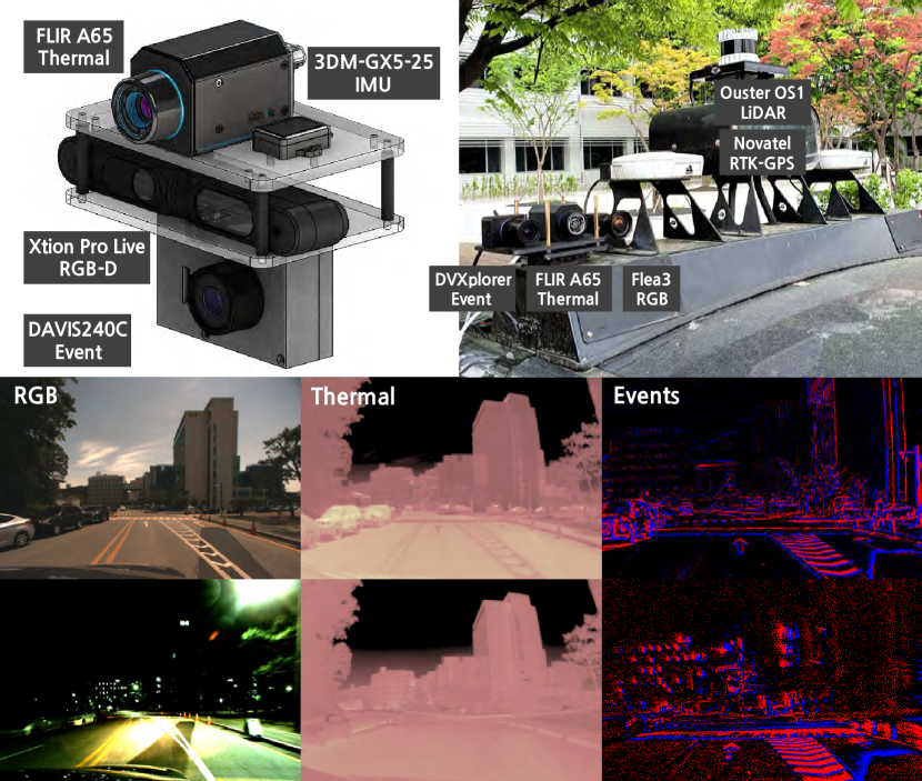
Figure 1: An overview of the sensor system and the dataset. We set up different sensor configurations for handheld (upper left) and driving (upper right). Sensor systems include RGB, thermal, events, depth, and interial measurements. Each sensor is indicated with the letter box. Each sensor’s visibility differences are displayed in the lower row. Relative to RGB, thermal and event show less variance to the illumination condition.

Public datasets provide large environmental variations from cameras. Some of them provide measurements from indoor [1, 2, 3] and the others arrange outdoor scenes [4, 5, 6] providing a large scale of sensor measurements. Synthetic datasets [7, 8, 9] were also provided for diversity.

However, achieving robust visual SLAM under low visibility still remains challenging. For typical cameras that collect information by integrating photons during the exposure time, the captured image is concentrated on the lighting more than the object. Thus, the ideas of collecting information from visual domains other than visible light intensity have been introduced. The alternative vision sensors have advantages over typical cameras. For instance, the thermal cameras could capture infrared radiation, and the event cameras [10] could detect temporal changes. These special abilities make the sensor measurement to be more independent from external lighting and motion conditions. For datasets including alternative vision sensors, event datasets [11, 12, 13, 14, 15, 16] and thermal datasets [17, 18] were publicly released.

In this paper, we present a dataset for developing robust visual SLAM in the real world by providing:

• the first dataset to enclose information from multiple types of aligned alternative vision sensors;

• multi-sensory measurements with ground-truth from external positioning system and generated from SLAM;

• wide range of environments in indoor and outdoor, recorded from multiple platforms.

II Related Works

II-A Related Datasets

Vision sensors produce a wide range of information, but they are easily influenced by external factors such as illumination and motion. As a result, a visual SLAM must be evaluated in a wide range of scenarios. Existing datasets cover a wide range of scenarios and include a large number of sensors, so as to develop robust SLAM algorithms. Various datasets, encompassing a wide range of environments, were released, including a wide range of visual and structural scenes. These datasets served as benchmark baselines and enabled the advancements for research.

In TUM RGB-D [1], image and depth data were collected, with ground-truths from the motion capture system. To gradually test the robustness of visual sensors over movement, sequences were separated by the motion speed. Similarly, in EuRoC [2], images from stereo cameras were measured along with IMU (IMU) and ground-truth. They separated the sequences with the difficulty of camera motion to test the robustness over kinematic variances. Further in SceneNet [8], photo-realistic videos, including motion blur and nonlinear camera response were provided with ground-truth. In InteriorNet [9], a large scale of synthetic environment with various customizable parameters, i.e., texture, illumination, artificial lights, motion blur, etc., were presented with a wide choice of sensors such as depth, fisheye, and event cameras. In NCLT [19] and TUM monoVO [20], a large scale of indoor and outdoor data with light and weather changes, was provided for long-term visual SLAM. Including all the variances mentioned above in urban environment, datasets such as KITTI [4], Cityscapes [5], and Complex urban dataset [6] were suggested.

Although many studies already covered a wide range of real-world noises, the problem of classical cameras, which are highly dependent on external light, remains. To overcome the appearance change and motion problem of conventional cameras, datasets using alternative vision sensors, such as thermal and event cameras, were also introduced.

II-B Alternative Vision Datasets

Unlike conventional cameras that capture intensity from the visible light spectrum, thermal cameras capture infrared intensity from object surfaces. The infrared measurements are generally more dependent on the object’s temperature than external light; thermal cameras can capture the scene information independently from external light conditions. Further, the event cameras [10] are visual sensors that capture relative luminance changes over time, not the absolute intensity. To code the instant light changes while maintaining low latency, the event camera uses a particular type of data representation: streams of tuples, not the sequence of images. Thus, the sensors’ output characteristics are distinctive from typical cameras. The event cameras require unique methods to process data, and several datasets have been released.

TABLE I: Comparison with previous alternative vision datasets

Dataset			Sensor
	Intensity	Depth	Thermal	Event	GT
Mueggler et al. [12]	✓			✓	✓
MVSEC [13]	✓	✓		✓	✓
UZH-FPV [14]	✓			✓	✓
DSEC [16]	✓	✓		✓	✓
Fischer et al. [15]	✓			✓	✓
Maddern et al. [17]	✓		✓		✓
Choi et al. [18]	✓	✓	✓		✓
ViViD++ (proposed)	✓	✓	✓	✓	✓

In early stages, [11] combined eDVS sensor with depth sensor and released data in indoor sequences. Later the Event-Camera Dataset and Simulator [12] was released, enabling the simulated events and widening the selection of test environments.

MVSEC [13] is a dataset with various lighting and motion measured with stereo event camera and inertial sensors. The dataset contains a large variety of condition changes, suggesting the utilization of the event camera for high-speed motion estimation. However, the dataset does not include repeated measurements in outdoor environments. In UZH-FPV [14], aggressively moving drones were used to provide event camera data for extreme motion cases. Also, a large-scale event camera dataset was presented in [16], covering most of applicable environments.

To investigate the appearance change problem with the event camera, in the Brisbane-Event-VPR dataset [15], the event camera was mounted on the car and acquired data along the same trajectory at different times. The dataset provides a large appearance change due to sun elevation changes. Especially in midnight sequences, street lights largely affect the cameras, and VPR becomes nearly impossible, opening a problem to robustly run event-based algorithms under both motion and appearance changes.

Also for thermal cameras, datasets covering illumination changes have been released. In [17], the handheld rig of RGB, thermal, and GPS (GPS) receiver was constructed, and collected data at different times. For object detection in thermal images, Then, KAIST Multi-Spectral Day/Night Dataset [18] have presented a sensor system including stereo RGB, LiDAR, and thermal camera for SLAM purposes. Their data were collected with GPS at a large scale and along with daytime temperature changes.

As listed above, several datasets have provided environmental variances with different types of sensors in various environments. However, as in Table I, none of the datasets include multi-sensor configurations for solving motion disturbances and illumination conditions together, which are two significant variances in the real world. We insist that both sensors should be utilized for complementing each other because thermal cameras are more robust by less dependency on external light sources, and event cameras are better for extreme motion cases. Therefore we compose a dataset with multiple types of visual information, at different wavelengths and temporal intensity difference, along with depth measurements and ground-truth for SLAM.

TABLE II: Sensor specifications and data types

Sensors	Specifications	Topic name	Description	Message type
Thermal	FLIR A65 640×512 pixel, 30Hz / 20Hz (handheld) FOV : 90 °vert., 69 °horiz. Spectral Range : 7.5-13 $\mu$m	/thermal/camera_info /thermal/image_raw	Header Image (16bit, 1ch)	sensor_msgs/CameraInfo sensor_msgs/Image
RGB-D	Asus Xtion Pro Live 640×480 pixel, 30Hz FOV : 45 °vert., 58 °horiz.	/depth/camera_info /depth/image_raw /rgb/camera_info /rgb/image	Header Image (16bit, 1ch) Header Image (8bit, 3ch)	sensor_msgs/CameraInfo sensor_msgs/Image sensor_msgs/CameraInfo sensor_msgs/Image
RGB	Flea®3 FL3-U3-13E4C-C 1280×1024 pixel, 60Hz FOV : 89 °vert., 73.8 °horiz.	/camera/camera_info /camera/image_color	Header Image (8bit, 3ch)	sensor_msgs/CameraInfo sensor_msgs/Image
Event	Handheld : DAVIS 240C 240×180 pixel, upto 12 MEPS Driving : DVXplorer 640×480 pixel, upto 165 MEPS	/dvs/events	Event	dvs_msgs/EventArray
GPS	NovAtel Pwrpak7 E-1 VEXXIS GNSS-500 Dual Antenna	/gps /bestpos	GPS	gps_common/GPSFix novatel_gps_msgs/NovatelPosition
Inertial	LORD Microstrain 3DM-GX5-25 On-board IMU (MPU 6150) On-board IMU (MPU 9250) On-board IMU (InvenSense ICM-20948)	/imu/data /dvs/imu /dvs/imu /os1_cloud_node/imu	IMU	sensor_msgs/Imu
LiDAR	Handheld : Velodyne VLP-16 Driving : Ouster OS1-64	/velodyne_point_cloud /os1_cloud_node/points	Pointcloud	sensor_msgs/PointCloud2

III Environment

III-A Sensors and Data types

We setup different types of vision sensors: RGB, thermal, and event. As mentioned in Fig. 1, we configured different sensor systems for handheld and driving sequences. In both scenarios, the three types of visual sensors were included, but details differ. IMU was installed for handheld, and the depth sensor was changed from depth camera to LiDAR for outdoor because we observed that the depth measurements of a structured light depth camera were unreliable on the outside. The dataset is provided with the binary format in rosbag. The rostopic names, sensor model, and specifications are listed in Table II. The timestamp from the clock running on each sensor frame, was initialized to rostime at startup and recorded in the header of each message. For the thermal camera, FLIR A65 was used with the raw format of 16 bits instead of the typical 8 bits. Note that the actual bits used for image demonstration are 14 bits due to two empty bits in the front. The non-uniformity-correction (NUC) was set to manual and done at the beginning of each sequence but not during the experiment. For the event camera, different sensors were used for each setup. DAVIS240C, which produces events and intensity images, was used for handheld sequences. And DVXplorer, with higher spatial resolution but without intensity images, was used for driving sequences. The LiDARs used for each system also differs. Velodyne LiDAR with 16 channels and 100m range was used for handheld sequences, and Ouster LiDAR with 64 channels and 120m range was used for driving sequences.

III-B Ground-Truth Generation

III-B1 Handheld indoor

A cortex motion capture system KARPE (KAIST Arena with Real-time Positioning Environment) [21] was used to track the sensor system’s 6 Degree of Freedom (DoF) pose. The system uses multiple infrared strobes to track the reflected light from the markers, assigning marker IDs to each track. The ID given to each marker did not change during the experiment, and the minimum number of markers to compose a 6DoF tracking was three. To ensure a robust track, we installed additional markers over the minimum number. As the motion capture system only provides the position of each marker, not the rotation, we defined the 6DoF marker frames from the tracked position of markers and provided them as the ground-truth.

III-B2 Handheld outdoor

We have generated poses for handheld outdoor sequences because the motion capture system was only available with preinstalled indoor equipment, and the GPS receiver was not able to solve the precise location in the experiment site. Thus as an evaluation baseline, we used the pointcloud from scans of VLP-16 attached to the top of the sensor jig and generated pose with LOAM variants [22][23] with scan context [24] for loop closure.

III-B3 Driving

With the dual antenna RTK-GPS installed on the car roof, we obtained a precise RTK-GPS position as the ground-truth. To ensure the validity of Global Navigation Satellite System (GNSS), the status of the calculated position was also recorded with the $/bestpos$ topic.

III-C Calibration

For calibration results, we offered a chain of relative poses between sensors. The sensor chains were connected to the RGB(-D) camera for both handheld and driving sensor systems, except for the on-board IMU sensors. More details of sensor layout, sample results, sequence statistics, and the validity of calibration can be found on the dataset homepage: https://visibilitydataset.github.io/.

III-C1 Calibration between cameras and external IMU

The relative poses between the cameras and an external IMU were estimated by moving the sensor system in front of the checkerboard and the grid of AprilTag [25], and calibrated with Kalibr [26]. Also the temporal offset between the RGB camera and the IMU was estimated by correlating the angular velocity norms of the sensors. The results of extrinsic calibration are shown in Fig. 2.

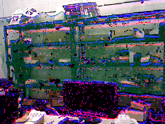
(a) RGB-D pointcloud projected
to event frames in the handheld seq.

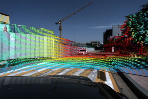
(b) LiDAR pointcloud projected
to RGB frames in the driving seq.

Figure 2: Pointclouds transformed into the other cameras, by the calibration results. In (b), LiDAR pointclouds are psudocolored with the depth values.

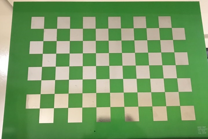
(a) RGB image of
PCB checkerboard.

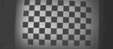
(b) Thermal image of
heated PCB.

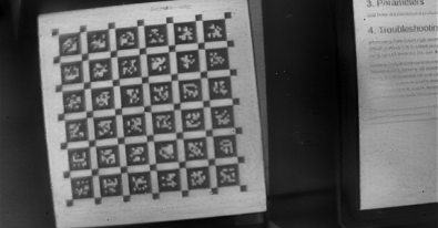
(c) Image of AprilTag
recovered from events.

Figure 3: Checkerboard pattern used for extrinsic calibration between alternative vision sensors. In (b), the difference in the heat dissipation rate of each material results in a temperature pattern. In (c), an intensity image is reconstructed from events using E2VID [27] and used for calibration.

III-C2 Calibration of thermal camera

Because the thermal camera only captures the temperature but not the intensity difference, a special type of checkerboard was required to make the pattern detectable for both intensity and thermal cameras. We used a calibration board made of aluminum coating on the printed circuit board (PCB) as in Fig. 3(a). To produce detectable edges in the thermal camera, the board was heated before calibration. Because the heat dissipation of aluminum is higher than plastic, the aluminum pattern is cooled faster and showed a lower temperature. Then the checkerboard pattern became visible from both RGB and thermal cameras as in Fig. 3(b), enabling the thermal camera to be calibrated as the same procedure of the RGB camera.

III-C3 Calibration of event cameras

The DAVIS240C event camera in the handheld sequences produces an intensity image, enabling image-based calibration. However, in the driving sequences, the DVXplorer event camera did not have images. Thus we chose to use reconstructed intensity images from events, using E2VID [27]. With the reconstructed AprilTag images as in Fig. 3(c), the event camera could be calibrated as the same way RGB camera was calibrated.

III-C4 Calibration between LiDAR and camera

The RGB camera in the handheld sequences contains depth measurements from structured light. Thus the transformation between a LiDAR and a camera could be directly computed by running ICP (ICP) [28] on the pointclouds obtained from both sensors. The transformation is obtained by matching planes and edges from each sensor. For best results, we have collected measurements at the intersection of three orthogonal planes for calibration. The relative poses of sensors were calculated by aligning orthogonal plane points.

In the driving sequences, the extrinsic parameter between a LiDAR and a RGB camera was found by minimizing reprojection errors of the marker board plane extracted from a LiDAR and a camera. The extrinsic transformation is $4\times 4$ homogenous transform matrix $\mathbf{T}^{rgb}_{lidar}$, that transforms all points from the LiDAR to the RGB frame. We captured $i$ numbers of snapshots with fully visible checkerboard on both the camera and the LiDAR. Then, the extrinsic calibration was calculated with both point-wise Euclidean and plane vector distance. The distances are defined as $\mathbf{D}_{point}=\left\lVert{\mathbf{\hat{n}}_{rgb}\cdot(\mathbf{p}_{rgb}-\mathbf{T}^{rgb}_{lidar}\mathbf{p}_{lidar})}\right\rVert$ and $\mathbf{D}_{vector}=d(\mathbf{\hat{n}}_{rgb},\mathbf{T}^{rgb}_{lidar}\mathbf{\hat{n}}_{lidar})$, where $\mathbf{p}_{rgb}$, $\mathbf{\hat{n}}_{rgb}$ are plane points and normals from the RGB camera, and $\mathbf{p}_{lidar}$, $\mathbf{\hat{n}}_{lidar}$ are plane points and normals from the LiDAR, and $d$ is a quaternion distance. Then the extrinsic could be found by solving the following minimization problem: $\operatorname*{argmin}_{\mathbf{T}^{rgb}_{lidar}}\sum_{i}(\mathbf{D}_{i,point}+\mathbf{D}_{i,vector})$. The temporal offset between a LiDAR and sensor system was calculated by comparing the trajectory obtained from LiDAR and visual odometry. Given the extrinsic calibration between LiDAR and camera from the method mentioned above, the temporal offset was estimated by minimizing the Average Trajectory Error (ATE) [29] upon different temporal offset values.

III-C5 Calibration between marker ground-truth and sensor system

The calibration between the motion capture system and the camera was achieved by comparing the marker’s 6DoF path of the sensor measurements. We defined a virtual marker frame using four markers, and compared the marker frame trajectory with the camera poses estimated by recording a checkerboard. The relative transformation between the marker frame and the camera was obtained by following Hand-Eye Calibration [30]. We defined the camera frame and the marker frame at time $t$ as $\mathbf{T}_{Ct}$ and $\mathbf{T}_{Mt}$, and the transformation of the marker frame from the camera as $\mathbf{T}_{CM}$. Then we solve the following equation: $\mathbf{T}^{~{}}_{Ci}\mathbf{T}^{~{}}_{CM}\mathbf{T}^{-1}_{Mi}=\mathbf{T}^{~{}}_{Cj}\mathbf{T}^{~{}}_{CM}\mathbf{T}^{-1}_{Mj}$. Also, then using relative poses $\mathbf{T}_{Lij}=\mathbf{T}^{-1}_{Lj}\mathbf{T}^{~{}}_{Li}$ and $\mathbf{T}_{Mij}=\mathbf{T}^{-1}_{Mj}\mathbf{T}^{~{}}_{Mi}$, the equation is reformulated into $\mathbf{T}_{Cij}\mathbf{T}_{CM}=\mathbf{T}_{CM}\mathbf{T}_{Mij}$. Then we obtain the form of solving $A=\mathbf{T}B\mathbf{T}^{-1}$ for $n$ pairs, and find error-minimizing transformation $\mathbf{T}_{CM}$. The temporal offset between ROS and the motion capture system was calculated for each sequence, by correlating the angular velocity norms of the IMU and the motion capture poses [31].

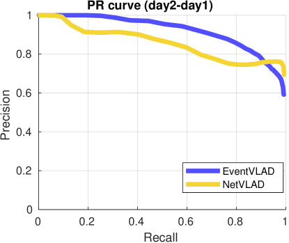
(a) PR curves of campus-day1 seq.
matched to campus-day2 DB.

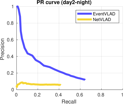
(b) PR curves of campus-night seq.
matched to campus-day2 DB.

Figure 4: VPR performances of event(blue) and RGB(yellow) cameras, trained with images from all of other “day” sequences and tested on the Campus sequences. By consisting a DB only with Campus-Day2, we tested the robustness of VPR module to match Campus-Day1/Night images to DB. The event-based VPR has shown more robustness over appearance changes.

IV Dataset

We recorded multiple repetitions along similar trajectories under distinct illumination conditions and motion constraints. To show the robustness of alternative vision sensors over illumination conditions, we have shown the performance of event-based VPR [32] in Fig. 4. To overview the sequences, 3D reconstructions and samples are in the figures: Figs. 5 and 6 for handheld and Figs. 7 and 8 for driving.

IV-A Handheld sequences

TABLE III: Environment setting for handheld sequences

Location	Illumination	Motion	Duration	GT
Indoor	Global	Slow	52.5s	Vicon
		Unstable	23.9s
		Aggressive	16.9s
	Dark	Slow	35.0s
		Unstable	20.5s
		Aggressive	16.9s
	Local	Slow	35.0s
		Unstable	17.1s
		Aggressive	13.4s
	Varying	Slow	35.8s
Outdoor	Day1	Slow	117s	LOAM (baseline)
	Day2	Slow	108s
	Night1	Slow	101s
	Night2	Slow	104s

For handheld sequences, we recorded multiple sessions in indoor and outdoor environments, respectively. In Fig. 6, the trajectory and sample scene images are displayed. The full sequence list is detailed in Table III.

For handheld indoor, sequences were divided by the level of motion deviation and lighting conditions. We have repeated trajectories at three different motion levels (42.7 to 120.7^∘/s), which are slow, unstable, and aggressive. Further, for each motion, we changed the illumination condition, from light turned on (global), turned off (dark), and flashlight on (local). We also included a bonus sequence (varying) to gradually change the flashlight intensity from dark to local. The sensor system’s global poses were captured via a motion capture system with 12 motion capture cameras mounted on the wall. The scale of the room was $12.3\text{\,}\mathrm{m}$ $\times$ $8.9\text{\,}\mathrm{m}$.

For handheld outdoor, we trailed the same trajectory at different times clockwise and counterclockwise. The approximate size of the space was about $60\text{\,}\mathrm{m}$ $\times$ $40\text{\,}\mathrm{m}$. In the environment, GPS was not sufficient because multi-story buildings enclosed the experiment site and yielded a multipath reception problem [33]. However, we were able to obtain LiDAR odometry from the plenty of planar and edge structures at the building.

IV-B Driving sequences

TABLE IV: Environment setting for driving sequences

Type	Location	Time	Duration	GT
Vision +LiDAR	Campus (3.6km)	Day1	445s	GPS, LOAM
		Day2	463s
		Evening	438s
		Night	445s
	City (9.3km)	Day1	914s
		Day2	1218s
		Evening	832s
		Night	840s
Vision	Campus (3.6km)	Morning	495s	GPS
		Day1	667s
		Day2	484s
		Evening	487s
		Night	443s
	City (9.3km)	Morning	858s
		Day1	1037s
		Day2	890s
		Evening	1127s
		Night	855s
	Urban (3.8km)	Morning	652s
		Day	785s
		Evening	593s
		Night	598s

For driving sequences, we repeated measurements along the predefined trajectories at different times. The repetitions were done throughout the entire day and night to enclose sun elevation changes. The appearances of the same place broadly change at different times, as seen in Fig. 8. The path was carefully selected to include visual loop closure, and the recording was done repeatedly over identical paths.

We set up three different trajectories, around the campus, in the urban canyon, and along the city’s arterial road. Each of the sequences was named as Campus, City, and Urban in Table IV. The campus sequence consisted of pedestrians, bicycles, and medium-rise buildings. In the city sequences, the vehicle drives along the river, under and over the bridges, and underpasses. In the urban sequences, the sensor observed high-rise buildings and tall trees (urban canyon). To provide extra data for unsupervised or self-supervised learning, we prepared “Vision” sequences recorded only with cameras without a LiDAR. To ensure reproducibility, we recommend to use the Campus sequences for validation, as in the setup of Fig. 4. Each traverse was from 3.6 to 9.3km long, with a maximum linear and angular velocity of 95 km/h and 39 ^∘/s. As the sun elevation angle changes, shadows differ, and large color shifts occurred in the evening scenes. Further, at night, artificial lights, including street lamps, were turned on. These illumination changes made the urban city very different from itself along the time of the day. Although the vehicle followed the same trajectory, the average speed dropped to 65% by the traffic signals and traffic congestion.

V Issues

The spectral response of the DAVIS240C used for our experiment overlaps with the infrared wavelength used from Cortex motion capture system. Thus, directly using DAVIS240C in the motion capture room resulted in an event camera’s high malfunction, capturing all the flashes of infrared strobes and ruining the event measurement. Therefore, we attached a C-Mount IR cut filter in front of the event camera to remove the effects of motion capture strobes.

The event cameras possess very high sensitivity and provide a high dynamic range from their relative form of luminance illustration. However, due to the sensitivity, we identified that the event camera produced erroneous output and decreased data quality when directly observing the light source. As is shown in the last column of Fig. 8, the event camera shows artifacts from the street lamps and loses visual information near the lamp. Further studies are required to neglect artifacts and recover the dynamic range of events.

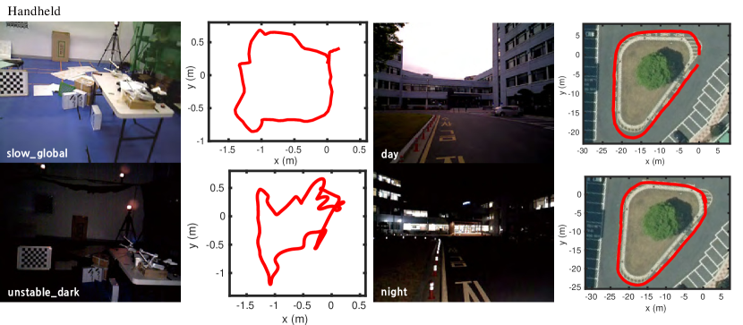
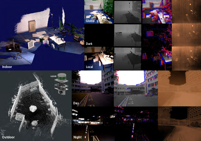
Figure 5: The samples of appearance changes and corresponding ground-truth or baseline trajectories (motion capture for indoor, SLAM for outdoor) from handheld sequences. For indoor trajectories, the measurements were done in the same room, but with different illumination and motion speed. Outdoor sequences were recorded by walking around the environment in a clockwise and counter-clockwise direction at different times.

Figure 6: Handheld scene overview with 3D reconstruction of the environment. From left to right, sampled images from RGB, depth, event and thermal camera are shown. The text label at each row represents illumination condition. The indoor environment was reconstructed with known poses from a motion capture and a RGB-D camera, and the outdoor was reconstructed by LeGO-LOAM run from VLP-16 LiDAR attached at the top of the sensor system.

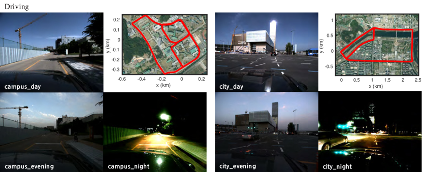
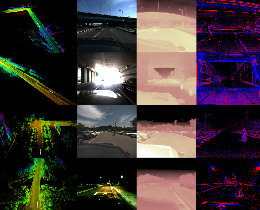
Figure 7: The samples of appearance changes and corresponding GPS trajectories from Vision for Visibility Dataset driving sequences. Outdoor sequences were recorded by following predefined path, at different times. Due to the illumination changes, visible appearance largely shifts as in the figure.

Figure 8: Vision+LiDAR sequences of City and Campus, with reconstruction from A-LOAM and the current viewpoint indicated with a white arrow. In the city, road infrastructures such as overpass and underpass / high-rise and large buildings / riverside are included. In the campus, parked cars / vegetation / medium-sized buildings / construction sites are observed. We could observe the light artifacts from the street lamps, in the last row of the event outputs.

VI Conclusion

This paper provides a vision for visibility dataset to overcome poor lighting conditions in robotics applications: beyond the visible light spectrum and temporal luminance differences. Besides providing a reference environment to test the performance of the thermal and event cameras, our dataset enables researchers to determine the vision sensors’ required abilities for robotic applications: fully identifying the potential of passive cameras in the real world. We hope our work will help solve robust robot vision regardless of motion or environmental disturbances by encouraging visual SLAM based on alternative vision sensors, proposing a test-bed to test optimal camera characteristics in the real world.

References

- Sturm et al. [2012] J. Sturm, N. Engelhard, F. Endres, W. Burgard, and D. Cremers, “A benchmark for the evaluation of RGB-D SLAM systems,” in Proc. IEEE/RSJ Intl. Conf. on Intell. Robots and Sys., 2012.
- Burri et al. [2016] M. Burri, J. Nikolic, P. Gohl, T. Schneider, J. Rehder, S. Omari, M. W. Achtelik, and R. Siegwart, “The EuRoC micro aerial vehicle datasets,” The International Journal of Robotics Research, vol. 35, no. 10, pp. 1157–1163, 2016.
- Jeon et al. [2021] J. Jeon, S. Jung, E. Lee, D. Choi, and H. Myung, “Run your visual-inertial odometry on nVidia Jetson: Benchmark tests on a micro aerial vehicle,” IEEE Robotics and Automation Letters, vol. 6, no. 3, pp. 5332–5339, 2021.
- Geiger et al. [2012] A. Geiger, P. Lenz, and R. Urtasun, “Are we ready for autonomous driving? the KITTI vision benchmark suite,” in Proc. IEEE Conf. on Comp. Vision and Pattern Recog., 2012.
- Cordts et al. [2016] M. Cordts, M. Omran, S. Ramos, T. Rehfeld, M. Enzweiler, R. Benenson, U. Franke, S. Roth, and B. Schiele, “The cityscapes dataset for semantic urban scene understanding,” in Proc. IEEE Conf. on Comp. Vision and Patt. Recog., 2016.
- Jeong et al. [2019] J. Jeong, Y. Cho, Y.-S. Shin, H. Roh, and A. Kim, “Complex urban dataset with multi-level sensors from highly diverse urban environments,” The International Journal of Robotics Research, vol. 38, no. 6, pp. 642–657, 2019.
- Handa et al. [2014] A. Handa, T. Whelan, J. McDonald, and A. Davison, “A benchmark for RGB-D visual odometry, 3D reconstruction and SLAM,” in Proc. IEEE Intl. Conf. on Robotics and Automation, ICRA, Hong Kong, China, May 2014.
- McCormac et al. [2017] J. McCormac, A. Handa, S. Leutenegger, and A. J. Davison, “SceneNet RGB-D: Can 5m synthetic images beat generic imageNet pre-training on indoor segmentation?” in Proc. of the IEEE International Conference on Computer Vision, 2017.
- Li et al. [2018] W. Li, S. Saeedi, J. McCormac, R. Clark, D. Tzoumanikas, Q. Ye, Y. Huang, R. Tang, and S. Leutenegger, “Interiornet: Mega-scale multi-sensor photo-realistic indoor scenes dataset,” in Proc. British Machine Vision Conference, 2018.
- Berner et al. [2013] R. Berner, C. Brandli, M. Yang, S.-C. Liu, and T. Delbruck, “A 240 180 10mw 12us latency sparse-output vision sensor for mobile applications,” in Proc. Symp. on VLSI Circ., 2013.
- Weikersdorfer et al. [2014] D. Weikersdorfer, D. B. Adrian, D. Cremers, and J. Conradt, “Event-based 3D SLAM with a depth-augmented dynamic vision sensor,” in Proc. IEEE International Conference on Robotics and Automation (ICRA), 2014, pp. 359–364.
- Mueggler et al. [2017] E. Mueggler, H. Rebecq, G. Gallego, T. Delbruck, and D. Scaramuzza, “The event-camera dataset and simulator: Event-based data for pose estimation, visual odometry, and slam,” The Intl. Journal of Robotics Research, 2017.
- Zhu et al. [2018] A. Z. Zhu, D. Thakur, T. Özaslan, B. Pfrommer, V. Kumar, and K. Daniilidis, “The multivehicle stereo event camera dataset: An event camera dataset for 3D perception,” IEEE Robotics and Automation Letters, vol. 3, no. 3, pp. 2032–2039, 2018.
- Delmerico et al. [2019] J. Delmerico, T. Cieslewski, H. Rebecq, M. Faessler, and D. Scaramuzza, “Are we ready for autonomous drone racing? the UZH-FPV drone racing dataset,” in Proc. IEEE Int. Conf. Robot. Autom. (ICRA), 2019.
- Fischer and Milford [2020] T. Fischer and M. Milford, “Event-based visual place recognition with ensembles of temporal windows,” IEEE Robotics and Automation Letters, vol. 5, no. 4, pp. 6924–6931, 2020.
- Gehrig et al. [2021] M. Gehrig, W. Aarents, D. Gehrig, and D. Scaramuzza, “Dsec: A stereo event camera dataset for driving scenarios,” IEEE Robotics and Automation Letters, vol. 6, pp. 4947–4954, 2021.
- Maddern and Vidas [2012] W. Maddern and S. Vidas, “Towards robust night and day place recognition using visible and thermal imaging,” in Proc. RSS 2012 Workshop: Beyond laser and vision: Alternative sensing techniques for robotic perception, 2012.
- Choi et al. [2018] Y. Choi, N. Kim, S. Hwang, K. Park, J. S. Yoon, K. An, and I. S. Kweon, “KAIST multi-spectral day/night data set for autonomous and assisted driving,” IEEE Trans. Intell. Transport. Sys., vol. 19, no. 3, pp. 934–948, 2018.
- Carlevaris-Bianco et al. [2015] N. Carlevaris-Bianco, A. K. Ushani, and R. M. Eustice, “University of Michigan North Campus long-term vision and LiDAR dataset,” International Journal of Robotics Research, vol. 35, no. 9, pp. 1023–1035, 2015.
- Engel et al. [2016] J. Engel, V. Usenko, and D. Cremers, “A photometrically calibrated benchmark for monocular visual odometry,” arXiv preprint arXiv:1607.02555, 2016.
- Kim et al. [2014] H.-Y. Kim, J.-S. Lee, H.-L. Choi, and J.-H. Han, “Autonomous formation flight of multiple flapping-wing flying vehicles using motion capture system,” Aerospace Science and Technology, vol. 39, pp. 596–604, 2014.
- Shan and Englot [2018] T. Shan and B. Englot, “LeGO-LOAM: Lightweight and ground-optimized LiDAR odometry and mapping on variable terrain,” in Proc. IEEE/RSJ Intl. Conf. on Intell. Robots and Sys., 2018, pp. 4758–4765.
- [23] https://github.com/HKUST-Aerial-Robotics/A-LOAM.
- Kim and Kim [2018] G. Kim and A. Kim, “Scan context: Egocentric spatial descriptor for place recognition within 3D point cloud map,” in Proc. IEEE/RSJ Intl. Conf. on Intell. Robots and Sys., 2018, pp. 4802–4809.
- Olson [2011] E. Olson, “AprilTag: A robust and flexible visual fiducial system,” in Proc. IEEE International Conference on Robotics and Automation, May 2011, pp. 3400–3407.
- Furgale et al. [2012] P. Furgale, T. D. Barfoot, and G. Sibley, “Continuous-time batch estimation using temporal basis functions,” in Proc. IEEE International Conference on Robotics and Automation, ICRA, 2012, pp. 2088–2095.
- Rebecq et al. [2019] H. Rebecq, R. Ranftl, V. Koltun, and D. Scaramuzza, “Events-to-video: Bringing modern computer vision to event cameras,” Proc. IEEE Conf. Comput. Vis. Pattern Recog., 2019.
- Besl and McKay [1992] P. J. Besl and N. D. McKay, “Method for registration of 3-D shapes,” in Sensor fusion IV: control paradigms and data structures. Intl. Society for Optics and Photonics, 1992.
- Zhang and Scaramuzza [2018] Z. Zhang and D. Scaramuzza, “A tutorial on quantitative trajectory evaluation for visual(-inertial) odometry,” in Proc. IEEE/RSJ Intl. Conf. on Intell. Robots and Sys., 2018.
- Daniilidis [1999] K. Daniilidis, “Hand-eye calibration using dual quaternions,” The Intl. Journal of Robotics Research, pp. 286–298, 1999.
- Furrer et al. [2018] F. Furrer, M. Fehr, T. Novkovic, H. Sommer, I. Gilitschenski, and R. Siegwart, “Evaluation of combined time-offset estimation and hand-eye calibration on robotic datasets,” Field and Service Robotics, pp. 145–159, 2018.
- Lee and Kim [2021] A. J. Lee and A. Kim, “EventVLAD: Visual place recognition with reconstructed edges from event cameras,” in Proc. IEEE/RSJ Intl. Conf. on Intell. Robots and Sys., 2021.
- Kos et al. [2010] T. Kos, I. Markezic, and J. Pokrajcic, “Effects of multipath reception on gps positioning performance,” in Proc. IEEE Conf. Intl. Symposium on Electronics in Marine, 2010.