Moiré disorder effect in twisted bilayer graphene

Abstract

We theoretically study the electronic structure of magic-angle twisted bilayer graphene with disordered moiré patterns. By using an extended continuum model incorporating non-uniform lattice distortion, we find that the local density of states of the flat band is hardly broadened, but splits into upper and lower subbands in most places. The spatial dependence of the splitting energy is almost exclusively determined by the local value of the effective vector potential induced by heterostrain, whereas the variation of local twist angle and local moiré period give relatively minor effects on the electronic structure. We explain the exclusive dependence on the local vector potential by a pseudo Landau level picture for the magic-angle flat band, and we obtain an analytic expression of the splitting energy as a function of the strain amplitude.

I introduction

Twisted bilayer graphene (TBG) exhibits various exotic quantum phenomena with a wide variety of correlated phases [1; 2; 3; 4; 5; 6; 7; 8; 9; 10; 11; 12; 13; 14; 15; 16; 17; 18; 19]. These quantum states originate from moiré-induced flat bands, which emerge when two graphene layers stacked with a magic-angle ($\sim 1^{\circ}$)[20; 21; 22; 23]. The flat band is usually described by a theoretical model assuming a regular moiré superlattice with a perfect periodicity [21; 22; 20; 23; 24; 25; 26; 27; 28; 29; 30; 31; 32; 33; 34; 35]. However, the moiré interference pattern is highly sensitive to a slight distortion of underlying structure. In TBG, an atomic displacement of graphene’s lattice is magnified in the moiré superlattice by factor of the inverse twist angle [36], leading to unavoidable disorder in the moiré superlattice. Indeed, the moiré patterns in actual TBG samples are not perfectly regular, but exhibit non-uniform structures including local distortion and variance of the twist angle [5; 6; 7; 4; 37; 38; 39; 40; 41; 42; 43; 44; 45; 46; 47; 48; 49; 50; 51].

It is expected that such a disorder in the moiré pattern would strongly affect the flat band and its electronic properties in the one-body level. Generally, non-uniform moiré systems are hard to treat theoretically, because one needs to consider a number of moiré periods each of which contains huge number of atoms. In previous works, the effect of the twist angle disorder in TBG was investigated using various theoretical approaches, such as a real-space domain model composed of regions with different twist angles [52], transmission calculations through one-dimensional variation of twist angle [53; 54; 55], and a Landau-Ginzburg theory to study the interplay between electron-electron interactions and disorder [56].

Figure 1: Moiré patterns of magic-angle TBG $(\theta=1.05^{\circ})$ with random non-uniform distortion of $\epsilon=0$, $0.0006$, $0.0012$ and $0.0018$, where the characteristic wave length is $\lambda=7L_{M}$, and the super-cell size (big parallelogram) is $n_{\rm SM}=8$. The bright region represents local AA stack and the dark region represents AB/BA stack. The red dots are the AA spots of the non-distorted TBG for reference.

In this paper, we study the electronic structure of magic-angle TBG in the presence of non-uniform moiré patterns as shown in Fig. 1, generated from random lattice distortion of graphene layers. The model automatically contains possible moiré disorder components, including various types of local strains and local rotations. We calculate the energy spectrum by using an extended continuum model incorporating non-uniform lattice distortion [57]. We find that the local density of states (LDOS) of the flat band is hardly broadened but splits place by place. Remarkably, the spatial variation of the splitting energy is totally uncorrelated with local twist angle or local periodicity, but it is almost exclusively determined by the local value of the effective vector potential caused by heterostrain, or relative strains between layers. We explain the exclusive dependence on the strain-induced vector potential by using a pseudo Landau level picture for the magic-angle flat band [58], and obtain an analytic expression for the splitting energy as a function of the strain amplitude. The strain-induced flat band splitting is an analog of that in uniformly-distorted TBGs [59; 60; 61; 5; 62; 63; 64; 65], and the strong coincidence between the splitting energy and the local strain tensor in non-uniform TBGs reflects a highly-localized feature of the flat band wave function.

This paper is organized as follows. Before we consider non-uniform moiré disorder, we present in Sec. II a detailed study on a TBG with uniform distortion. We investigate the effects of different types of strain components independently, and show that the flat band splitting is mainly caused by shear and anisotropic-normal heterostrain. We derive an approximate expression for the splitting energy by using the pseudo Landau level analysis. In Sec. III, we calculate the LDOS of magic-angle TBG with non-uniform moiré patterns, and demonstrate a strong relationship between the LDOS split and the strain-induced vector potential. A brief conclusion is given in Sec. IV.

II TBG with a uniform distortion

II.1 Atomic structure

We first consider a TBG with a uniform lattice distortion and investigate its effect on the flat band. We define the lattice vectors of monolayer graphene as $\bm{a}_{1}=a(1,0)$ and $\bm{a}_{2}=a(1/2,\sqrt{3}/2)$ where $a=0.246$ nm is the lattice constant, and define $\bm{b}_{j}$ as the corresponding reciprocal lattice vectors to satisfy $\bm{a}_{i}\cdot\bm{b}_{j}=\delta_{ij}$. In a perfect TBG without distortion, the lattice vectors of layer $l(=1,2)$ are given by $\bm{a}_{j}^{(l)}=R(\mp\theta/2)\bm{a}_{j}$ where $\mp$ is for $l=1$ and $2$, respectively, $R$ is a two-dimensional rotation matrix, and $\theta$ is the twist angle.

We introduce a uniform distortion to layer $l$, whch is expressed by a matrix,

$$\mathcal{E}^{(l)}=\begin{pmatrix}\epsilon^{(l)}_{xx}&-\Omega^{(l)}+\epsilon^{(l)}_{xy}\\ \Omega^{(l)}+\epsilon^{(l)}_{xy}&\epsilon^{(l)}_{yy}\end{pmatrix}.$$ (1)

The $\mathcal{E}^{(l)}$ represents a deformation such that a carbon atom at a position $\bm{r}$ in a non-distorted system is shifted to $\bm{r}+\mathcal{E}^{(l)}\bm{r}$. Here $\epsilon_{xx}^{(l)}$ and $\epsilon_{yy}^{(l)}$ represent normal strains in $x$ and $y$ directions, respectively, $\epsilon_{xy}^{(l)}$ is a shear strain, and $\Omega^{(l)}$ is a rotation from the original twist angle For later arguments, we also define the isotropic/anisotropic components of the normal strain by

$$\epsilon_{\pm}^{(l)}=\frac{1}{2}(\epsilon_{xx}^{(l)}\pm\epsilon_{yy}^{(l)}),$$ (2)

and the interlayer difference of each strain/rotation component as

$$\epsilon_{\pm} =\epsilon_{\pm}^{(1)}-\epsilon_{\pm}^{(2)},$$

$$\epsilon_{xy} =\epsilon_{xy}^{(1)}-\epsilon_{xy}^{(2)},$$

$$\Omega =\Omega^{(1)}-\Omega^{(2)}.$$ (3)

In the presence of distortion, the lattice vectors change to $\bm{a}_{j}^{(l)}=(1+\mathcal{E}^{(l)})R(\mp\theta/2)\bm{a}_{j}$. In the following, we assume the original twist angle and the distortion is sufficiently small ($\theta,\Omega^{(l)},\epsilon^{(l)}_{\mu\nu}\ll 1$), so that

$$\bm{a}_{j}^{(l)}\approx\bigl{[}R\left(\mp\theta/2\right)+\mathcal{E}^{(l)}\bigr{]}\bm{a}_{j}.$$ (4)

Similarly, the reciprocal lattice vectors are written as

$$\bm{b}_{j}^{(l)} \approx\bigl{[}R\left(\mp\theta/2\right)-\mathcal{E}^{(l)\rm T}\bigr{]}\bm{b}_{j},$$ (5)

where $T$ is the matrix transpose.

In an intrinsic monolayer graphene, six corner points of the Brillouin zone (BZ) are given by $\xi\bm{K}_{j}\,(j=1,2,3)$, where $\xi=\pm 1$ label the valley degree of freedom, and

$$\bm{K}_{j} =R\left(\phi_{j}\right)\frac{4\pi}{3a}(-1,0),\quad\phi_{j}=\frac{2\pi}{3}(j-1),$$ (6)

are equivalent points in the BZ. Corresponding vectors for the disroted TBG are written as

$$\bm{K}_{j}^{(l)} \approx\bigl{[}R\left(\mp\theta/2\right)-\mathcal{E}^{(l)\rm T}\bigr{]}\bm{K}_{j}.$$ (7)

Figure 2 illustrates the schematics of BZ for (a) a non-distorted TBG and (b) a distorted TBG. In each panel, blue and orange hexagons on the left represent the first BZ of graphene layer $l=1$ and 2, respectively, where the corner points are given by $\xi\bm{K}_{j}^{(l)}$. We define interlayer shift of the corner points by

$$\bm{q}_{j}=\bm{K}_{j}^{(1)}-\bm{K}_{j}^{(2)}\quad(j=1,2,3),$$ (8)

as shown in Fig. 2. The $\bm{q}_{j}$’s can be expressed only by the interlayer rotation and strain components as

$$\bm{q}_{j} =\frac{4\pi}{3a}\left[R\left(\phi_{j}\right)\begin{pmatrix}\epsilon_{+}\\ \theta-\Omega\end{pmatrix}+R\left(-\phi_{j}\right)\begin{pmatrix}\epsilon_{-}\\ \epsilon_{xy}\end{pmatrix}\right].$$ (9)

The reciprocal lattice vectors of the moiré pattern are given by $\bm{G}^{M}_{j}=\bm{b}^{(1)}_{j}-\bm{b}^{(2)}_{j}$, which are also written as $\bm{G}^{\rm M}_{1}=\bm{q}_{2}-\bm{q}_{1}$, $\bm{G}^{\rm M}_{2}=\bm{q}_{3}-\bm{q}_{2}$. In Fig. 2, a green hexagon on the right side represents the moiré Brillouin zone defined by $\bm{G}^{\rm M}_{j}$’s

II.2 Continuum model and Band calculation

We use the continuum model [33; 34; 22; 24; 28; 25; 26; 27; 60; 29; 30; 31; 32; 62; 63; 61; 57; 58; 59; 60; 61; 62; 63; 64; 65; 35; 66; 67] to describe a strained TBG. The effective Hamiltonian for valley $\xi$ is written as

$${\cal H}^{(\xi)}(\bm{k})=\left(\begin{array}[]{cc}H_{1}(\bm{k})&U^{\dagger}\\ U&H_{2}(\bm{k})\end{array}\right),$$ (12)

where $H_{l}(\bm{k})$ is the $2\times 2$ Hamiltonian of distorted monolayer graphene, and $U$ is the interlayer coupling matrix. The Hamiltonian[Eq. (12)] works on the four-component wave function $(\psi_{A}^{(1)},\psi_{B}^{(1)},\psi_{A}^{(2)},\psi_{B}^{(2)})$, where $\psi_{X}^{(l)}$ represents the envelope function of sublattice $X(=A,B)$ on layer $l(=1,2)$.

The $H_{l}(\bm{k})$ is given by

$$H_{l}(\bm{k})=-\hbar v\left[\left(R\left(\mp\theta\right)+\mathcal{E}^{(l)}\right)^{-1}\left(\bm{k}+\frac{e}{\hbar}\bm{A}^{(l)}\right)\right]\cdot\bm{\sigma},$$ (13)

where $\mp$ is for $l=1$ and $2$, respectively, $v$ is the graphene’s band velocity, $\bm{\sigma}=\left(\xi\sigma_{x},\sigma_{y}\right)$ and $\sigma_{x}$, $\sigma_{y}$ are the Pauli matrices in the sublattice space $\left(A,B\right)$. We take $\hbar v/a=2.14$ eV [25]. The $\bm{A}^{(l)}$ is the strain-induced vector potential that is given by [68; 69; 70]

$$\bm{A}^{(l)} = \xi\frac{3}{2}\frac{\beta\gamma_{0}}{ev}\begin{pmatrix}\epsilon_{-}^{(l)}\\ -\epsilon_{xy}^{(l)}\ \end{pmatrix},$$ (14)

where $\gamma_{0}=2.7$ eV is the nearest neighbor transfer energy of intrinsic graphene and $\beta\approx 3.14$. Note that the strain-induced vector potential, Eq. (14), depends only on $\epsilon_{-}^{(l)}$ and $\epsilon_{xy}^{(l)}$, while not on $\epsilon_{+}^{(l)}$ or $\Omega^{(l)}$.

The interlayer coupling matrix $U$ is given by

$$U=\sum_{j=1}^{3}U_{j}\mathrm{e}^{\mathrm{i}\xi\bm{q}_{j}\cdot\bm{r}},$$

$$U_{1}=\left(\begin{array}[]{cc}u&u^{\prime}\\ u^{\prime}&u\end{array}\right),\quad U_{2}=\left(\begin{array}[]{cc}u&u^{\prime}\omega^{-\xi}\\ u^{\prime}\omega^{+\xi}&u\end{array}\right),$$ (19)

$$U_{3}=\left(\begin{array}[]{cc}u&u^{\prime}\omega^{+\xi}\\ u^{\prime}\omega^{-\xi}&u\end{array}\right).$$ (22)

The parameters $u=79.7$ meV and $u^{\prime}=95.7$ meV are interlayer coupling strength between AA/BB and AB/BA stack region, respectively. The difference between $u$ and $u^{\prime}$ effectively arise from the in-plane lattice relaxation and from the out-of-plane corrugation effect [25; 57]. The interlayer matrix $U$ depends on the strain via $\bm{q}_{j}$’s [Eq. (9)].

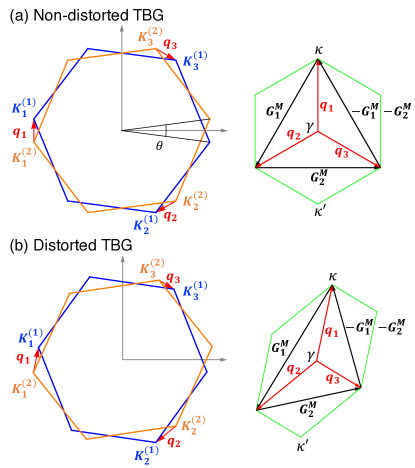
Figure 2: Brillouin zones of (a) a non-distorted TBG and (b) a distorted TBG. Blue and orange hexagons on the left represent the first Brillouin zone of graphene layer 1 and 2 (twisted by $\mp\theta/2$), respectively, and red arrows are the displacement vectors from the layer 2’s $K_{+}$ point to layer 1’s. A green hexagon on the right side is the moiré Brillouin zone.

Below we investigate the effect of lattice distortion on the energy bands using the effective Hamiltonian, Eq. (12). In fact, the electronic structure is mainly affected by the interlayer asymmetric components of the strain tensor [Eq. (II.1)] , and in particular, the flat band is highly sensitive to $\epsilon_{-}$ and $\epsilon_{xy}$. To demonstrate this, we calculate the energy bands of the magic-angle TBG $(\theta=1.05^{\circ})$ in the presence of asymmetric strain $\mathcal{E}^{(1)}=-\mathcal{E}^{(2)}=\mathcal{E}/2$, where different types of strain components $\Omega,\epsilon_{+},\epsilon_{-},\epsilon_{xy}$ are considered independently. Figure 3 shows the band dispersion and the density of state (DOS) in individual strain components, where black, green, red, and blue lines represent the strain amplitude (i.e., value of $\Omega,\epsilon_{+},\epsilon_{-},\epsilon_{xy}$) of $0,0.001,0.002$ and $0.004$, respectively.

We clearly observe that the central flat band is particularly sentsitive to $\epsilon_{-}$ and $\epsilon_{xy}$, where a small distortion of 0.001 leads to a significant split of the flat band about 20 meV. In constrast, $\epsilon_{+}$ and $\Omega$ gives relatively minor effects. $\epsilon_{+}$ moves the Dirac points at $\kappa$ and $\kappa^{\prime}$ in the opposite directions in energy, resulting in a smaller DOS split. $\Omega$ shifts the twist angle from the magic angle and slightly broadens the flat band. The strain-induced flat band splitting was also found the previous work, which considered the effect of uniaxial heterostrain in TBG [60; 5; 62; 63], which corresponds to $\epsilon_{-}$ and $\epsilon_{xy}$ in our notation.

It should also be noted that the split flat bands in Fig. 3 are not completely separated, but stick together at certain points near $\gamma$ (off the path shown in Fig. 3) [60]. These Dirac points are originally located at $\kappa$ and $\kappa^{\prime}$ in the non-distorted TBG, and when a uniform distortion is applied, they move without gap opening under the protection of the $C_{2z}T$ symmetry. The two Dirac points cannot pair-annihilate because they have the same Berry phase [71].

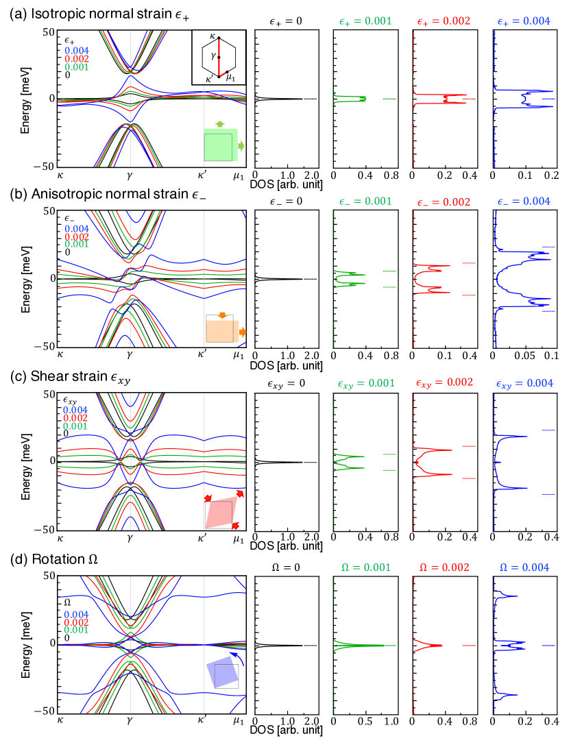
Figure 3: Band structure and the DOS of uniformly distorted magic-angle TBGs with different types of strain components, $\epsilon_{+},\epsilon_{-},\epsilon_{xy},\Omega$. Different colors represent different amplitudes of strain. horizontal lines in the right panels (DOS) indicate energies of the split levels in the pseudo Landau level picture.

II.3 Pseudo Landau Level approximation

As shown in the previous section, the flat band is split significantly by anisotropic normal strain $\epsilon_{-}$ and shear strain $\epsilon_{xy}$, while not much by other components. We explain this by using the pseudo Landau level picture of TBG [58], which describes the flat band as the Landau level (LL) under a moiré-induced fictitious magnetic field. We apply the same formulation to the strained TBG, Eq. (12), and analytically estimate the flat-band split energy.

The pseudo-LL Hamiltonian is obtained by rewriting the Hamiltonian matrix [Eq. (12)] in the basis $(\psi^{+}_{A},\psi^{+}_{B},\psi^{-}_{A},\psi^{-}_{B})$ where $\psi^{\pm}_{X}=(\psi^{(1)}_{X}\pm\mathrm{i}\psi^{(2)}_{X})/\sqrt{2}$, and then expanding it in $\bm{r}$ with respect to the origin (the AA-point) upto the first order [58]. We ignore $\left(R\left(\mp\theta/2\right)+\mathcal{E}^{(l)}\right)^{-1}$ in Eq. (13), which gives only higher order effects. The detailed calculation is presented in Appendix A.

As a result, the effective Hamiltonian is written as

$$H_{\rm PLL}=\left(\begin{array}[]{cc}H_{+}&V^{\dagger}\\ V&H_{-}\end{array}\right),$$ (26)

where

$$H_{\pm}=-\hbar v\left(\bm{k}\pm\frac{e}{\hbar}\bm{a}(\bm{r})\right)\cdot\bm{\sigma},$$ (27)

$$\bm{a}(\bm{r})=\xi\frac{2\pi u^{\prime}}{eva}(\theta-\Omega)\left(\begin{array}[]{c}-y\\ x\end{array}\right).$$ (30)

Eq. (27) is essentially the Dirac Hamiltonian under a uniform magnetic field $\nabla\times(\pm\bm{a})=(0,0,\pm b_{\rm eff})$ with $b_{\rm eff}=\xi[4\pi u^{\prime}/(e^{2}va)](\theta-\Omega)$. Note that the pseudo vector potential $\bm{a}(\bm{r})$ originates from the inter-sublattice coupling $u^{\prime}$ in the moiré interlayer Hamiltonian [Eq. (II.2)], and it should be distinguished from the strain-induced vector potential $\bm{A}^{(l)}$.

The off-diagonal matrix $V$ is given by

$$V=\left(-3\mathrm{i}uI_{2}-\frac{ev}{2}\bm{A}\cdot\bm{\sigma}\right)\mathrm{e}^{-\mathrm{i}\frac{2e}{\hbar}\chi(\bm{r})},$$ (31)

where $I_{2}$ is a $2\times 2$ identity matrix, $u$ is the intra-sublattice coupling in moiré interlayer Hamiltonian [Eq. (II.2)], and

$$\bm{A}=\bm{A}^{(1)}-\bm{A}^{(2)}=\xi\frac{3}{2}\frac{\beta\gamma_{0}}{ev}\begin{pmatrix}\epsilon_{-}\\ -\epsilon_{xy}\end{pmatrix},$$ (32)

$$\chi(\bm{r})=\xi\frac{\pi u^{\prime}}{eva}\left[(x^{2}+y^{2})\epsilon_{+}+(x^{2}-y^{2})\epsilon_{-}+xy\epsilon_{xy}\right].$$ (33)

Here $\bm{A}^{(l)}$ is the strain-induced vector potential argued in the previous section.

In the absence of the off-diagonal matrix $V$, the eigenstates are given by the pseudo LLs of sector $H_{\pm}$. For $\xi=+$ valley, it is explicitly written as

$$|+,0,m\rangle=\begin{pmatrix}0\\ \varphi_{0,m}\\ 0\\ 0\end{pmatrix},\quad|-,0,m\rangle=\begin{pmatrix}0\\ 0\\ \varphi_{0,m}\\ 0\end{pmatrix},$$ (34)

where $\varphi_{0,m}(\bm{r})\propto e^{-im\phi}e^{-r^{2}/(4l_{\rm eff}^{2})}$ is the 0th LL wavefunction with angular momentum $m$ expressed in the polar coordinate $\bm{r}=r(\cos\phi,\sin\phi)$, and $l_{\rm eff}=\sqrt{\hbar/(eb_{\rm eff})}$. The 0th LLs in Eq. (34) have exactly opposite sublattice polarization (i.e., $|+,0,m\rangle$ on B, and $|-,0,m\rangle$ on A), because the Dirac Hamiltonians $H_{\pm}$ have opposite pseudo magnetic fields $\pm b_{\rm eff}$.

In the absence of distortion ($\bm{A}=\chi=0$), the 0th LLs remain the zero-energy eigenstates even we include the off-diagonal terms $-3\mathrm{i}uI_{2}$ [Eq. (31)], because $I_{2}$ does not mix different sublattices. The flat band of TBG is understood by these degenerate 0th LLs. Since the effective Hamiltonian Eq. (34) is based on the linear expansion around $\bm{r}=0$ (the AA spot), the approximation is valid for the LL wavefunctions with small angular momenta $m$’s, which are well localized to $\bm{r}=0$.

When we switch on the disortion terms, the 0th Landau levels are immediately hybridized by $\bm{A}\cdot\bm{\sigma}$ in the off-diagonal matrix $V$, and split into $E=\pm\Delta E/2$, where

$$\Delta E=ev|\bm{A}|=\frac{3}{2}\beta\gamma_{0}\sqrt{\epsilon_{-}^{2}+\epsilon_{xy}^{2}}.$$ (35)

Note that the pseudo gauge potential $\chi(\bm{r})$ only contributes to the phase factor of the coupling matrix elements [Eq. (31)], giving a higher order correction to the splitting energy (see, Appendix A). Eq. (35) explains the exclusive dependence of the flat band splitting on $\epsilon_{-}$ and $\epsilon_{xy}$. Considering $(3/2)\beta\gamma_{0}\approx$ 13 eV, a distortion ($\epsilon_{-},\epsilon_{xy})$ of the order of $10^{-3}$ corresponds to a split width $\Delta E\sim$ 10 meV.

In Fig. 3, horizontal red lines represent $\pm\Delta E/2$ of Eq. (35), showing a good agreement with the actual split width of the DOS. In the energy bands, the structures at $\kappa$, $\kappa^{\prime}$ and $\mu_{i}$ are nicely explained by this simple splitting picture. On the other hand, the energy bands around $\gamma$ point is rather complicated and cannot be captured by the same approximation. This is consistent with the fact that the wavefunction at $\gamma$ is extended over the entire moiré pattern unlike those at $\kappa$, $\kappa^{\prime}$ and $\mu_{i}$ concentrating on AA points [72; 73; 74; 75], and hence the pseudo LL approximation (assuming the localization at AA point) fails. The Dirac band touching mentioned above actually occurs near $\gamma$.

III TBG with non-uniform distortion

III.1 Theoretical modelling

In this section, we construct a theoretical model to simulate a non-uniform distortion in TBG. We consider a super moiré unit cell composed of $n_{\rm SM}\times n_{\rm SM}$ original moiré units ($n_{\rm SM}$: integer), and assume that the lattice distortion is periodic with the super period as illustrated in Fig. 1. The primitive lattice vectors for the super unit cell are given by $\bm{L}_{j}^{\rm SM}=n_{\rm SM}\bm{L}_{j}^{\rm M}$ and the corresponding reciprocal lattice vectors are $\bm{G}_{j}^{\rm SM}=\bm{G}_{j}^{\rm M}/n_{\rm SM}$.

We define the in-plane displacement vector of layer $l=1,2$ as

$$\bm{u}^{(l)}(\bm{r})=\sum_{\bm{p}}\bm{C}_{\bm{p}}^{(l)}\mathrm{e}^{-\left(\lambda\left|\bm{p}\right|/2\pi\right)^{2}}\mathrm{e}^{\mathrm{i}\bm{p}\cdot\bm{r}},$$ (36)

which represents a deformation such that a carbon atom of layer $l$ at a position $\bm{r}$ is shifted to $\bm{r}+\bm{u}^{(l)}(\bm{r})$. Here $\bm{p}$ runs over $\bm{p}=m_{1}\bm{G}^{\rm SM}_{1}+m_{2}\bm{G}^{\rm SM}_{2}$, and $\lambda$ is the characteristic wave length of the spatial dependence of $\bm{u}^{(l)}(\bm{r})$. The amplitude $\bm{C}_{\bm{p}}^{(l)}=(C_{\bm{p},x}^{(l)},C_{\bm{p},y}^{(l)})$ is a two-dimensional random vector which satisfy $\bm{C}_{\bm{-p}}^{(l)}=\bm{C}_{\bm{p}}^{(l)*}$ for real-valued $\bm{u}^{(l)}(\bm{r})$. We assume that different components of $\bm{C}_{\bm{p}}^{(l)}$ are totally uncorrelated such that

$$\langle C_{\bm{p},i}^{(l)}C_{\bm{p}^{\prime},j}^{(l^{\prime})*}\rangle=\delta_{l,l^{\prime}}\delta_{\bm{p},-\bm{p}^{\prime}}\delta_{i,j}C_{0}^{2},$$ (37)

where $\langle\rangle$ is the sampling average and $C_{0}$ is a length parameter to characterize the amplitude of the random displacement field.

The local strain tensors and the rotation angle can be expressed in terms of $\bm{u}^{(l)}(\bm{r})$ as

$$\epsilon^{(l)}_{ij}(\bm{r})=\frac{1}{2}\left(\partial_{i}u^{(l)}_{j}+\partial_{j}u^{(l)}_{i}\right)$$ (38)

$$\Omega^{(l)}(\bm{r})=\frac{1}{2}\left(\partial_{x}u^{(l)}_{y}-\partial_{y}u^{(l)}_{x}\right).$$ (39)

As in the uniform case, we define $\epsilon_{\pm}^{(l)}(\bm{r})$ by Eq. (2), and relative strain components $\epsilon_{\pm}(\bm{r}),\epsilon_{xy}(\bm{r}),\Omega(\bm{r})$ by Eq. (II.1). We introduce the magnitude of distortion, $\epsilon$, as the root mean square of the interlayer difference of the strain tensor elements [Eq. (II.1)], or,

$$\epsilon\equiv\sqrt{\langle|\epsilon_{\pm}|^{2}\rangle}=\sqrt{\langle|\epsilon_{xy}|^{2}\rangle}=\sqrt{\langle|\Omega|^{2}\rangle}=\sqrt{\frac{\pi^{3}}{2}\frac{C_{0}^{2}S_{\rm SM}}{\lambda^{4}}},$$ (40)

where $S_{\rm SM}=|\bm{L}_{1}^{\rm SM}\times\bm{L}_{2}^{\rm SM}|$ is the area of the super moiré unit cell.

Figure 1 show examples of distorted moiré patterns in the magic-angle TBG($\theta=1.05^{\circ}$) with different values of $\epsilon=$ 0, 0.0006, 0.0012, 0.0018, where $n_{\rm SM}=8$ (indicated by a big parallelogram) and $\lambda=7L_{M}$. We adopted a continuous color code to express the stacking sequence [76], where the bright region represents local AA stack and the dark region represents AB/BA stack. The red dots are the AA spots of the non-distorted TBG for reference. It should be noted that a small distortion in graphene lattice of the order of $\epsilon$ is magnified to the moiré disorder of $\epsilon/\theta\sim 60\epsilon$.

We calculate the energy spectrum by using an extended continuum model incorporating non-uniform lattice distortion [57]. The Hamiltonian is given by Eq. (12), where the diagonal blocks are replaced by

$$H_{l}(\bm{k})=-\hbar v\left(\bm{k}+\frac{e}{\hbar}\bm{A}^{(l)}(\bm{r})\right)\cdot\bm{\sigma},$$ (41)

with the local strain-induced vector potential

$$\bm{A}^{(l)}(\bm{r}) = \xi\frac{3}{2}\frac{\beta\gamma_{0}}{ev}\begin{pmatrix}\epsilon_{-}^{(l)}(\bm{r})\\ -\epsilon_{xy}^{(l)}(\bm{r})\ \end{pmatrix},$$ (42)

and the interlayer coupling $U$ is replaced with,

$$U=\sum_{j=1}^{3}U_{j}\,\mathrm{e}^{\mathrm{i}\xi[\bm{q}_{j}\cdot\bm{r}\,+\,\bm{K}_{j}\cdot(\bm{u}^{(2)}(\bm{r})-\bm{u}^{(1)}(\bm{r}))]}.$$ (43)

Here $U_{j}$ are defined in Eq. (II.2), $\bm{K}_{j}$ are the corner points of an intrinsic graphene [Eq. (6)] and $\bm{q}_{j}$ are interlayer corner-point shifts [Eq. (8)] of non-distorted TBG. In the diagonal matrix, we neglected the rotation matrix $\left(R\left(\mp\theta\right)+\mathcal{E}^{(l)}\right)^{-1}$ in Eq. (13), which gives a minor effect in the uniform distortion case.

While in this paper we focus on the in-plane components of lattice displacement, real TBG samples also contain out-of-plane corrugations [77; 78; 79]. The primary effect of the corrugation is to differentiate the lattice spacing of AA-stacking and AB-stacking regions, which is effectively incorporated by the difference between $u$ and $u^{\prime}$ parameters in the matrix $U$ [25; 57], as already mentioned. We may also have an additional effect from non-uniform corrugation, which is left for future work.

III.2 Energy spectrum and flat-band splitting

Using the model obtained above, we calculate the local density of states (LDOS) for the magic-angle TBG ($\theta=1.05^{\circ}$) with a randomly-generated displacement configuration $\bm{u}^{(l)}(\bm{r})$. First, we take $\epsilon=0.0004$, $\lambda=7L_{M}$, and $n_{\rm SM}=12$. Figure 4(a) illustrates the moiré structure, where the distortion is barely observed as a slight shift of AA points (yellow spots) with respect to the regular red dots. In Fig. 4(b), we plot the LDOS along line $XX^{\prime}$, which is defined by a broken line in Fig. 4(a). We can see that the LDOS of the flat band separates into upper and lower parts by a splitting energy depending on the position. This is quite different from the case of a random electrostatic potential which simply broadens the band width. Figure 4(d) shows the spatial distribution of the splitting energy $\Delta E$, which is defined by the energy distance between the two LDOS peaks. Here a hexagonal tile corresponds to a single moiré unit cell, and its color represents $\Delta E$ at the center of the hexagon (the AA point).

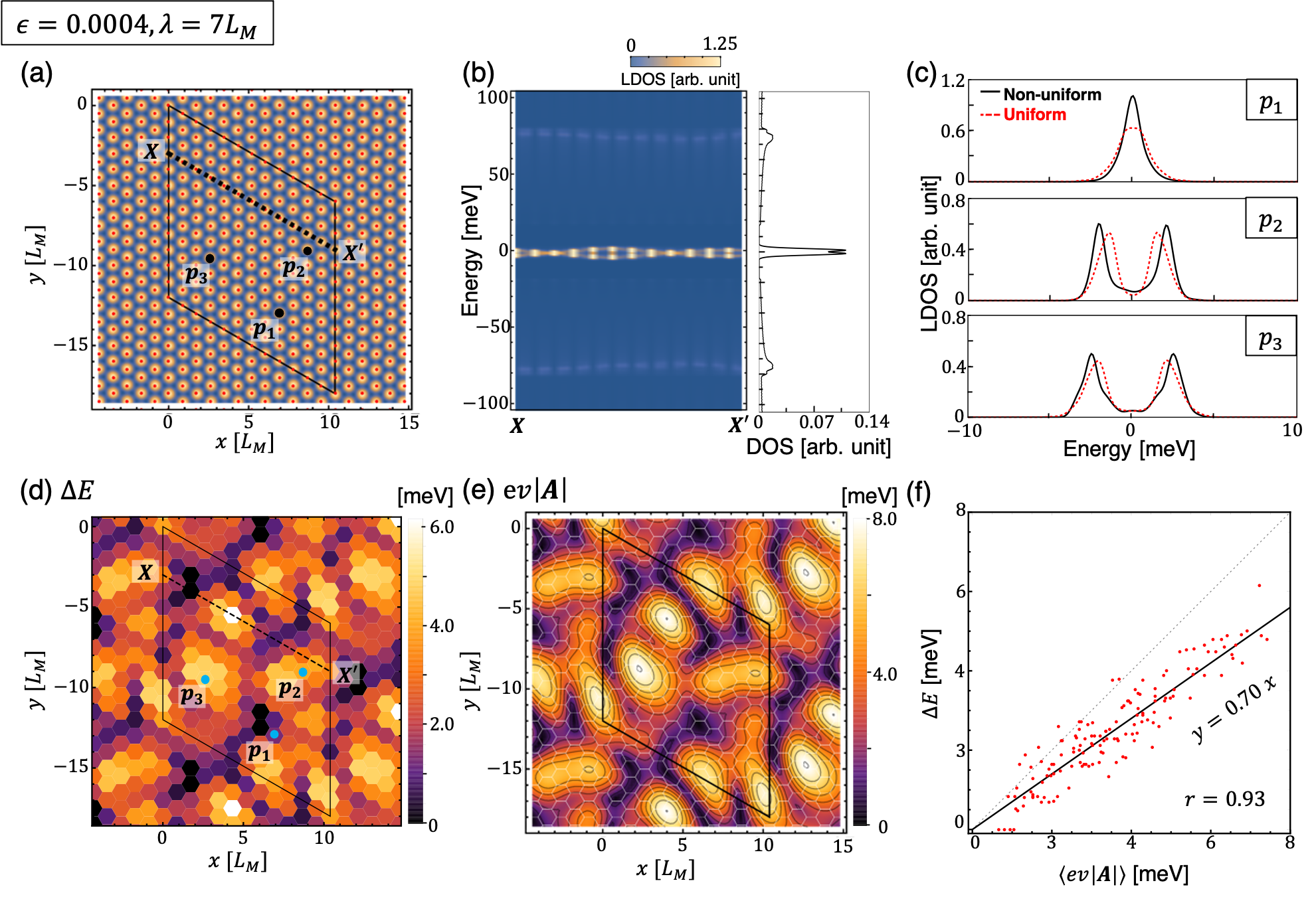
Figure 4: (a) Moiré pattern of a disordered magic-angle TBG with $\epsilon=0.0004,\lambda=7L_{\rm M}$. The distortion is observed as slight shifts of AA points (yellow spots) relative to the regular red dots. (b) LDOS along line $XX^{\prime}$ [defined by a broken line in (a)]. (c) (Black, solid) LDOS at the points of $p_{1},p_{2},p_{3}$ in (a). (Red, dashed) LDOS at the AA point of the corresponding uniform TBG with the strain tensors fixed to the local value. (d) The spatial distribution of the splitting energy $\Delta E$, or the energy distance between the two LDOS peaks. A hexagonal tile corresponds to a single moiré unit cell, and its color represents $\Delta E$ at the center of the hexagon (the AA point). (e) A contour plot of the interlayer difference of the strain-induced vector potential, $ev\left|\bm{A}(\bm{r})\right|$

. (f) A scattered plot of $\Delta E$ and $ev\left|\bm{A}\right|$ (averaged in every moiré unit cell).

Actually, the local split width of the flat band is almost solely determined by the local value of the interlayer difference of the strain-induced vector potential,

$$\bm{A}(\bm{r})=\bm{A}^{(1)}(\bm{r})-\bm{A}^{(2)}(\bm{r}),$$ (44)

and the local splitting energy is approximately given by $\Delta E\sim ev|\bm{A}(\bm{r})|$ as in the uniform case [Eq. (32)]. To demonstrate this, we show a contour plot of $ev\left|\bm{A}(\bm{r})\right|$ in Fig. 4(e). We observe a nearly perfect agreement with the distribution of $\Delta E$ in Fig. 4(d). We also present a scattered plot of $\Delta E$ and $ev\left|\bm{A}\right|$ (averaged in every moiré unit cell) in Fig. 4(f), where we have a high correlation coefficient $r\approx 0.93$, and a fitted line is given by $\Delta E\approx 0.7ev|\bm{A}|$. The strong correlation between the splitting width and the strain-induced vector potential is a special property of the magic-angle flat band, as it relies on its peculiar Landau level like wavefunction. On the other hand, the position of the satellite peaks (around $\pm 80$ meV in Fig. 4) is totally uncorrelated with $ev\left|\bm{A}\right|$ (the correlation coefficient about $r\sim 0.1$), but it is weakly correlated with the local twist angle $\Omega$ ($r\sim 0.5$).

These results suggest that the local electronic structure in the flat band region of non-uniform TBG is well described by a uniform Hamiltonian with the strain tensors fixed to the local value. In Fig. 4(c), we plot the LDOS of the non-uniform TBG at the points of $p_{1},p_{2},p_{3}$ in Fig. 4(a), and the local density of states of the corresponding uniform TBGs at AA point. Indeed, we see a nice agreement between the two curves. We also note that the LDOS is never completely gapped out at $E=0$, in accordance with the calculation of uniformly-strained TBGs where the two flat bands are always connected by the Dirac points.

The approximation with the local Hamiltonian is usually expected to be valid in a long-range limit with $\lambda\gg L_{M}$, but actually it works fairly well down to a short-ranged distortion. Figure 5 shows the plots similar to Fig. 4 calculated for different characteristic wave lengths, $\lambda=5L_{M},3L_{M},L_{M}$. The correlation coefficient between $\Delta E$ and $ev\left|\bm{A}\right|$ is found to be 0.90 at $\lambda=3L_{M}$, and it is still 0.73 at $\lambda=L_{M}$. We presume that it reflects the strongly localized feature of the flat-band wavefunctions.

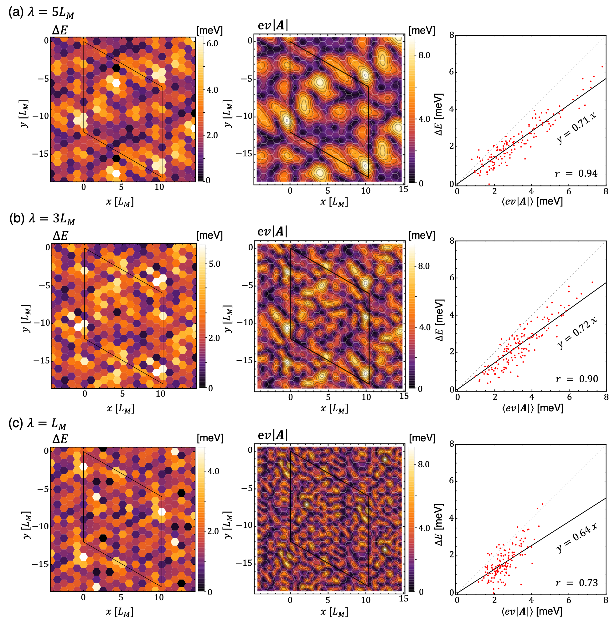
Figure 5: Plots similar to Figs. 4(d)-(f) calculated for different characteristic wave lengths $\lambda=5L_{M},3L_{M},L_{M}$.

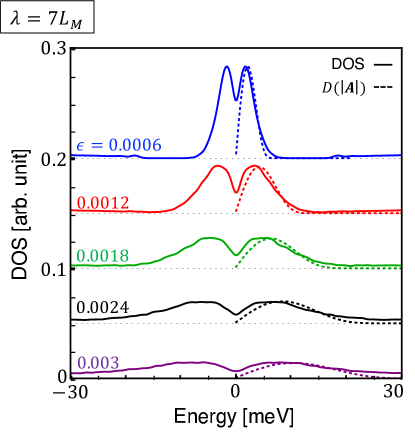
Figure 6: The total DOS of disordered magic-angle TBGs with different distortion amplitudes $\epsilon$. For each curve, we take an average over different random configurations. Broken lines are the distribution function $D(|\bm{A}|)$ with horizontal axis scaled by $E=0.7ev|\bm{A}|$.

Figure 6 plots the total DOS of non-uniform TBG in different distortion amplitudes $\epsilon$ with $\lambda=7L_{M}$, For each curve, we take an overage over different random configurations. We see that the two-level splitting feature in the LDOS still remains as a double peak structure in the total DOS. In increasing $\epsilon$, the curve is simply extended horizontally, as expected the relationship $\Delta E\sim ev|\bm{A}|$. The form of the DOS curve is roughly determined by the distribution function $D(|\bm{A}|)$, which is plotted as broken line in Fig. 6 for the current model. Here we scale the horizontal axis by $E=0.7ev|\bm{A}|$ in accordance with Fig. 4(f).

By using the formula Eq. (35), we can roughly estimate the flat band split energy in real TBG samples. In a recent local measurement of the magic-angle TBG [44] has shown that the local twist angle varies from $\theta=1.05^{\circ}$ to $1.18^{\circ}$, which amounts to $\Omega\simeq 0.001$ (rad). By assuming that the strain tensor elements, $\epsilon_{\pm}$, $\epsilon_{xy}$, $\Omega$ have comparable magnitudes, the typical value of the flat band split width on this sample is estimated at $\Delta E\simeq 10$ meV using Eq. (35). These results suggest that, in realistic magic-angle TBGs with non-uniform moiré disorder, the flat band is not actually a single band cluster but it splits by a sizable energy in most places. It is consistent with the STM measurements of TBGs near the magic angle [4; 7], where a significant separation of the LDOS was observed. The local flat-band separation may also be responsible for the pronounced Landau fan at the charge neutral point which is commonly observed in the transport experiments [2; 3; 10; 44], since the two separate bands are always touching as argued in Sec. II. The splitting of the flat band would affect the ground state properties in the presence of the electron-electron interaction, since the Hilbert space of the half-split flat band is different from the original full flat band.

While we focus on the strain effect in this calculation, the distortion of the moiré pattern should also give rise to a non-uniform electrostatic potential via an inhomogeneous charge distribution[72; 28; 80; 64]. We expect that the effect is roughly captured by including a local shift of the energy in the present calculation. At the filling factor $\nu=2$ (i.e. half-filling of the upper flat band), for instance, the upper LDOS peak would be aligned to the Fermi energy without changing the local splitting width, to achieve the homogeneous electron density of $\nu=2$. We leave a detailed calculation including the electrostatic potential for future works.

IV Conclusion

We have studied the electronic structure of the magic-angle TBG with non-uniform moiré distortion by using an extended continuum model. We found that the local density of states of the flat band is split by the local interlayer difference of anisotropic normal strain $\epsilon_{-}$ and shear strain $\epsilon_{xy}$, while isotropic strain $\epsilon_{+}$ and rotation $\Omega$ give relatively minor effects. The splitting of the flat band can well be described by a pseudo landau level picture for the magic-angle flat band, and an analytical expression of the splitting energy is obtained [Eq. (35)]. The coincidence between the splitting energy of the LDOS and the local strain is maintained even in a short-ranged distortion with $\lambda\sim L_{M}$, reflecting a highly-localized feature of the flat band wave function.

Appendix A Pseudo Landau Level Hamiltonian

In this appendix, we derive the pseudo landau level Hamiltonian Eq. (26) by applying the method of Ref. [58] to the disordered TBG. By defining

$$\psi^{\pm}_{X}=(\psi^{(1)}_{X}\pm\mathrm{i}\psi^{(2)}_{X})/\sqrt{2}\quad(X=A,B),$$ (45)

the Hamiltonian matrix of Eq. (12) is written in the basis $(\psi^{+}_{A},\psi^{+}_{B},\psi^{-}_{A},\psi^{-}_{B})$ as

$$H=\left(\begin{array}[]{cc}h_{+}+\displaystyle\frac{\mathrm{i}}{2}(U-U^{\dagger})&h_{-}+\displaystyle\frac{\mathrm{i}}{2}(U+U^{\dagger})\\ h_{-}-\displaystyle\frac{\mathrm{i}}{2}(U+U^{\dagger})&h_{+}-\displaystyle\frac{\mathrm{i}}{2}(U-U^{\dagger})\end{array}\right),$$ (48)

where

$$h_{+} =-\Biggl{(}\hbar v\bm{k}+ev\frac{\bm{A}^{(1)}+\bm{A}^{(2)}}{2}\Biggr{)}\cdot\bm{\sigma}$$

$$h_{-} =-ev\frac{\bm{A}^{(1)}-\bm{A}^{(2)}}{2}\cdot\bm{\sigma}.$$ (49)

In the following, we neglect the homostrain component $\bm{A}^{(1)}+\bm{A}^{(2)}$, and focus on the heterostrain part $\bm{A}=\bm{A}^{(1)}-\bm{A}^{(2)}$.

Since the wavefuncton of the flat band is localized around the AA region, we expand the interlayer coupling matrix $U(\bm{r})$ around the AA stacking point $(\bm{r}=0)$ to the linear order of $r/L_{M}$. As a result, we have

$$\frac{U+U^{\dagger}}{2} =\sum_{j=1}^{3}U_{j}\cos{\bm{q}_{j}\cdot\bm{r}}\approx 3uI_{2}$$ (50)

$$\mathrm{i}\frac{U-U^{\dagger}}{2} =\sum_{j=1}^{3}U_{j}\sin{\bm{q}_{j}\cdot\bm{r}}\approx\sum_{j=1}^{3}U_{j}\bm{q}_{j}\cdot\bm{r}.$$ (51)

By using Eqs. (51) and  (9), the diagonal part of the Hamiltonian (48) is written as

$$h_{+}\pm\displaystyle\frac{\mathrm{i}}{2}(U-U^{\dagger})=-\hbar v\left[\bm{k}\pm\frac{e}{\hbar}\left(\bm{a}(\bm{r})+\nabla\chi(\bm{r})\right)\right]\cdot\bm{\sigma}$$ (52)

where $\bm{a}(\bm{r})$ is the pseudo vector potential of Eq. (30) and the $\chi(\bm{r})$ is the gauge potential of Eq. (33). Finally, the effective Hamiltonian Eq. (26) is obtained by applying a gauge transformation,

$$\begin{pmatrix}\tilde{\psi}_{X}^{(+)}\\ \tilde{\psi}_{X}^{(-)}\ \end{pmatrix}=\left(\begin{array}[]{cc}\mathrm{e}^{-\mathrm{i}\frac{e}{\hbar}\chi}&0\\ 0&\mathrm{e}^{+\mathrm{i}\frac{e}{\hbar}\chi}\end{array}\right)\begin{pmatrix}\psi_{X}^{(+)}\\ \psi_{X}^{(-)}\ \end{pmatrix}.$$ (55)

The coupling matrix elements in the 0th LLs are given by

$$\langle-,0,m^{\prime}|V|+,0,m\rangle=\frac{ev}{2}\bm{A}\cdot\bm{\sigma}\langle\varphi_{0,m^{\prime}}|\mathrm{e}^{-\mathrm{i}\frac{2e}{\hbar}\chi(\bm{r})}|\varphi_{0,m}\rangle$$

$$\qquad\approx\frac{ev}{2}\bm{A}\cdot\bm{\sigma}\left[\delta_{m,m^{\prime}}-2\mathrm{i}\frac{e}{\hbar}\langle\varphi_{0,m^{\prime}}|\chi(\bm{r})|\varphi_{0,m}\rangle\right].$$ (56)

Therefore, the gauge potential $\chi$ only contributes to a higher order correction in the 0th LL splitting.

References

- Cao et al. [2018a] Y. Cao, V. Fatemi, A. Demir, S. Fang, S. L. Tomarken, J. Y. Luo, J. D. Sanchez-Yamagishi, K. Watanabe, T. Taniguchi, E. Kaxiras, R. C. Ashoori, and P. Jarillo-Herrero, Nature 556, 80 (2018a).
- Cao et al. [2018b] Y. Cao, V. Fatemi, S. Fang, K. Watanabe, T. Taniguchi, E. Kaxiras, and P. Jarillo-Herrero, Nature 556, 43 (2018b).
- Yankowitz et al. [2019] M. Yankowitz, S. Chen, H. Polshyn, Y. Zhang, K. Watanabe, T. Taniguchi, D. Graf, A. F. Young, and C. R. Dean, Science 363, 1059 (2019), https://www.science.org/doi/pdf/10.1126/science.aav1910 .
- Kerelsky et al. [2019] A. Kerelsky, L. J. McGilly, D. M. Kennes, L. Xian, M. Yankowitz, S. Chen, K. Watanabe, T. Taniguchi, J. Hone, C. Dean, A. Rubio, and A. N. Pasupathy, Nature 572, 95 (2019).
- Xie et al. [2019] Y. Xie, B. Lian, B. Jäck, X. Liu, C.-L. Chiu, K. Watanabe, T. Taniguchi, B. A. Bernevig, and A. Yazdani, Nature 572, 101 (2019).
- Jiang et al. [2019] Y. Jiang, X. Lai, K. Watanabe, T. Taniguchi, K. Haule, J. Mao, and E. Y. Andrei, Nature 573, 91 (2019).
- Choi et al. [2019] Y. Choi, J. Kemmer, Y. Peng, A. Thomson, H. Arora, R. Polski, Y. Zhang, H. Ren, J. Alicea, G. Refael, F. von Oppen, K. Watanabe, T. Taniguchi, and S. Nadj-Perge, Nature Physics 15, 1174 (2019).
- Sharpe et al. [2019] A. L. Sharpe, E. J. Fox, A. W. Barnard, J. Finney, K. Watanabe, T. Taniguchi, M. A. Kastner, and D. Goldhaber-Gordon, Science 365, 605 (2019), https://www.science.org/doi/pdf/10.1126/science.aaw3780 .
- Polshyn et al. [2019] H. Polshyn, M. Yankowitz, S. Chen, Y. Zhang, K. Watanabe, T. Taniguchi, C. R. Dean, and A. F. Young, Nature Physics 15, 1011 (2019).
- Lu et al. [2019] X. Lu, P. Stepanov, W. Yang, M. Xie, M. A. Aamir, I. Das, C. Urgell, K. Watanabe, T. Taniguchi, G. Zhang, A. Bachtold, A. H. MacDonald, and D. K. Efetov, Nature 574, 653 (2019).
- Cao et al. [2020] Y. Cao, D. Chowdhury, D. Rodan-Legrain, O. Rubies-Bigorda, K. Watanabe, T. Taniguchi, T. Senthil, and P. Jarillo-Herrero, Phys. Rev. Lett. 124, 076801 (2020).
- Serlin et al. [2020] M. Serlin, C. L. Tschirhart, H. Polshyn, Y. Zhang, J. Zhu, K. Watanabe, T. Taniguchi, L. Balents, and A. F. Young, Science 367, 900 (2020), https://www.science.org/doi/pdf/10.1126/science.aay5533 .
- Chen et al. [2020] G. Chen, A. L. Sharpe, E. J. Fox, Y.-H. Zhang, S. Wang, L. Jiang, B. Lyu, H. Li, K. Watanabe, T. Taniguchi, et al., Nature 579, 56 (2020).
- Saito et al. [2020] Y. Saito, J. Ge, K. Watanabe, T. Taniguchi, and A. F. Young, Nature Physics 16, 926 (2020).
- Zondiner et al. [2020] U. Zondiner, A. Rozen, D. Rodan-Legrain, Y. Cao, R. Queiroz, T. Taniguchi, K. Watanabe, Y. Oreg, F. von Oppen, A. Stern, et al., Nature 582, 203 (2020).
- Wong et al. [2020] D. Wong, K. P. Nuckolls, M. Oh, B. Lian, Y. Xie, S. Jeon, K. Watanabe, T. Taniguchi, B. A. Bernevig, and A. Yazdani, Nature 582, 198 (2020).
- Stepanov et al. [2020] P. Stepanov, I. Das, X. Lu, A. Fahimniya, K. Watanabe, T. Taniguchi, F. H. Koppens, J. Lischner, L. Levitov, and D. K. Efetov, Nature 583, 375 (2020).
- Arora et al. [2020] H. S. Arora, R. Polski, Y. Zhang, A. Thomson, Y. Choi, H. Kim, Z. Lin, I. Z. Wilson, X. Xu, J.-H. Chu, et al., Nature 583, 379 (2020).
- Stepanov et al. [2021] P. Stepanov, M. Xie, T. Taniguchi, K. Watanabe, X. Lu, A. H. MacDonald, B. A. Bernevig, and D. K. Efetov, Phys. Rev. Lett. 127, 197701 (2021).
- Suárez Morell et al. [2010] E. Suárez Morell, J. D. Correa, P. Vargas, M. Pacheco, and Z. Barticevic, Phys. Rev. B 82, 121407 (2010).
- Trambly de Laissardière et al. [2010] G. Trambly de Laissardière, D. Mayou, and L. Magaud, Nano letters 10, 804 (2010).
- Bistritzer and MacDonald [2011] R. Bistritzer and A. H. MacDonald, Proceedings of the National Academy of Sciences 108, 12233 (2011).
- Trambly de Laissardière et al. [2012] G. Trambly de Laissardière, D. Mayou, and L. Magaud, Phys. Rev. B 86, 125413 (2012).
- Lopes dos Santos et al. [2012] J. M. B. Lopes dos Santos, N. M. R. Peres, and A. H. Castro Neto, Phys. Rev. B 86, 155449 (2012).
- Koshino et al. [2018] M. Koshino, N. F. Q. Yuan, T. Koretsune, M. Ochi, K. Kuroki, and L. Fu, Phys. Rev. X 8, 031087 (2018).
- Kang and Vafek [2018] J. Kang and O. Vafek, Phys. Rev. X 8, 031088 (2018).
- Po et al. [2018] H. C. Po, L. Zou, A. Vishwanath, and T. Senthil, Phys. Rev. X 8, 031089 (2018).
- Guinea and Walet [2018] F. Guinea and N. R. Walet, Proceedings of the National Academy of Sciences 115, 13174 (2018), https://www.pnas.org/doi/pdf/10.1073/pnas.1810947115 .
- Bultinck et al. [2020] N. Bultinck, E. Khalaf, S. Liu, S. Chatterjee, A. Vishwanath, and M. P. Zaletel, Phys. Rev. X 10, 031034 (2020).
- Xie and MacDonald [2020] M. Xie and A. H. MacDonald, Phys. Rev. Lett. 124, 097601 (2020).
- Zhang et al. [2020] Y. Zhang, K. Jiang, Z. Wang, and F. Zhang, Phys. Rev. B 102, 035136 (2020).
- Liu and Dai [2021] J. Liu and X. Dai, Phys. Rev. B 103, 035427 (2021).
- Moon and Koshino [2013] P. Moon and M. Koshino, Phys. Rev. B 87, 205404 (2013).
- Koshino [2015] M. Koshino, New Journal of Physics 17, 015014 (2015).
- Carr et al. [2020] S. Carr, S. Fang, and E. Kaxiras, Nature Reviews Materials 5, 748 (2020).
- Cosma et al. [2014] D. A. Cosma, J. R. Wallbank, V. Cheianov, and V. I. Fal’Ko, Faraday Discussions 173, 137 (2014).
- Li et al. [2010] G. Li, A. Luican, J. M. B. Lopes dos Santos, A. H. Castro Neto, A. Reina, J. Kong, and E. Y. Andrei, Nat. Phys. 6, 109 (2010).
- Luican et al. [2011] A. Luican, G. Li, A. Reina, J. Kong, R. R. Nair, K. S. Novoselov, A. K. Geim, and E. Y. Andrei, Phys. Rev. Lett. 106, 126802 (2011).
- Brihuega et al. [2012] I. Brihuega, P. Mallet, H. González-Herrero, G. Trambly de Laissardière, M. M. Ugeda, L. Magaud, J. M. Gómez-Rodr$́\mathrm{i}$guez, F. Ynduráin, and J.-Y. Veuillen, Phys. Rev. Lett. 109, 196802 (2012).
- Wong et al. [2015] D. Wong, Y. Wang, J. Jung, S. Pezzini, A. M. DaSilva, H.-Z. Tsai, H. S. Jung, R. Khajeh, Y. Kim, J. Lee, S. Kahn, S. Tollabimazraehno, H. Rasool, K. Watanabe, T. Taniguchi, A. Zettl, S. Adam, A. H. MacDonald, and M. F. Crommie, Phys. Rev. B 92, 155409 (2015).
- Qiao et al. [2018] J.-B. Qiao, L.-J. Yin, and L. He, Phys. Rev. B 98, 235402 (2018).
- Yoo et al. [2019] H. Yoo, R. Engelke, S. Carr, S. Fang, K. Zhang, P. Cazeaux, S. H. Sung, R. Hovden, A. W. Tsen, T. Taniguchi, et al., Nature materials 18, 448 (2019).
- Shi et al. [2020] H. Shi, Z. Zhan, Z. Qi, K. Huang, E. v. Veen, J. Á. Silva-Guillén, R. Zhang, P. Li, K. Xie, H. Ji, M. I. Katsnelson, S. Yuan, S. Qin, and Z. Zhang, Nature Communications 11, 371 (2020).
- Uri et al. [2020] A. Uri, S. Grover, Y. Cao, J. A. Crosse, K. Bagani, D. Rodan-Legrain, Y. Myasoedov, K. Watanabe, T. Taniguchi, P. Moon, M. Koshino, P. Jarillo-Herrero, and E. Zeldov, Nature 581, 47 (2020).
- McGilly et al. [2020] L. J. McGilly, A. Kerelsky, N. R. Finney, K. Shapovalov, E.-M. Shih, A. Ghiotto, Y. Zeng, S. L. Moore, W. Wu, Y. Bai, K. Watanabe, T. Taniguchi, M. Stengel, L. Zhou, J. Hone, X. Zhu, D. N. Basov, C. Dean, C. E. Dreyer, and A. N. Pasupathy, Nature Nanotechnology 15, 580 (2020).
- Gadelha et al. [2021] A. C. Gadelha, D. A. Ohlberg, C. Rabelo, E. G. Neto, T. L. Vasconcelos, J. L. Campos, J. S. Lemos, V. Ornelas, D. Miranda, R. Nadas, et al., Nature 590, 405 (2021).
- Kazmierczak et al. [2021] N. P. Kazmierczak, M. Van Winkle, C. Ophus, K. C. Bustillo, S. Carr, H. G. Brown, J. Ciston, T. Taniguchi, K. Watanabe, and D. K. Bediako, Nature materials 20, 956 (2021).
- Tilak et al. [2021] N. Tilak, X. Lai, S. Wu, Z. Zhang, M. Xu, R. d. A. Ribeiro, P. C. Canfield, and E. Y. Andrei, Nature communications 12, 1 (2021).
- Mesple et al. [2021] F. Mesple, A. Missaoui, T. Cea, L. Huder, F. Guinea, G. Trambly de Laissardière, C. Chapelier, and V. T. Renard, Phys. Rev. Lett. 127, 126405 (2021).
- Huang et al. [2021] X. Huang, L. Chen, S. Tang, C. Jiang, C. Chen, H. Wang, Z.-X. Shen, H. Wang, and Y.-T. Cui, arXiv preprint arXiv:2102.08594 (2021).
- Schäpers et al. [2021] A. Schäpers, J. Sonntag, L. Valerius, B. Pestka, J. Strasdas, K. Watanabe, T. Taniguchi, M. Morgenstern, B. Beschoten, R. Dolleman, et al., arXiv preprint arXiv:2104.06370 (2021).
- Wilson et al. [2020] J. H. Wilson, Y. Fu, S. Das Sarma, and J. H. Pixley, Phys. Rev. Research 2, 023325 (2020).
- Padhi et al. [2020] B. Padhi, A. Tiwari, T. Neupert, and S. Ryu, Phys. Rev. Research 2, 033458 (2020).
- Joy et al. [2020] S. Joy, S. Khalid, and B. Skinner, Physical Review Research 2, 043416 (2020).
- Sainz-Cruz et al. [2021] H. Sainz-Cruz, T. Cea, P. A. Pantaleón, and F. Guinea, Phys. Rev. B 104, 075144 (2021).
- Thomson and Alicea [2021] A. Thomson and J. Alicea, Phys. Rev. B 103, 125138 (2021).
- Koshino and Nam [2020] M. Koshino and N. N. T. Nam, Phys. Rev. B 101, 195425 (2020).
- Liu et al. [2019] J. Liu, J. Liu, and X. Dai, Phys. Rev. B 99, 155415 (2019).
- Huder et al. [2018] L. Huder, A. Artaud, T. Le Quang, G. T. de Laissardière, A. G. M. Jansen, G. Lapertot, C. Chapelier, and V. T. Renard, Phys. Rev. Lett. 120, 156405 (2018).
- Bi et al. [2019] Z. Bi, N. F. Q. Yuan, and L. Fu, Phys. Rev. B 100, 035448 (2019).
- He et al. [2020] W.-Y. He, D. Goldhaber-Gordon, and K. T. Law, Nature communications 11, 1 (2020).
- Dai et al. [2021] Z.-B. Dai, Y. He, and Z. Li, Phys. Rev. B 104, 045403 (2021).
- Kaplan et al. [2022] D. Kaplan, T. Holder, and B. Yan, Phys. Rev. Research 4, 013209 (2022).
- Ochoa [2020] H. Ochoa, Phys. Rev. B 102, 201107 (2020).
- Parker et al. [2021] D. E. Parker, T. Soejima, J. Hauschild, M. P. Zaletel, and N. Bultinck, Phys. Rev. Lett. 127, 027601 (2021).
- Guinea and Walet [2019] F. Guinea and N. R. Walet, Physical Review B 99, 205134 (2019).
- Carr et al. [2019a] S. Carr, S. Fang, Z. Zhu, and E. Kaxiras, Physical Review Research 1, 013001 (2019a).
- Suzuura and Ando [2002] H. Suzuura and T. Ando, Phys. Rev. B 65, 235412 (2002).
- Pereira and Castro Neto [2009] V. M. Pereira and A. H. Castro Neto, Phys. Rev. Lett. 103, 046801 (2009).
- Guinea et al. [2010] F. Guinea, M. I. Katsnelson, and A. K. Geim, Nature Physics 6, 30 (2010).
- Liu et al. [2021] S. Liu, E. Khalaf, J. Y. Lee, and A. Vishwanath, Phys. Rev. Research 3, 013033 (2021).
- Rademaker and Mellado [2018] L. Rademaker and P. Mellado, Phys. Rev. B 98, 235158 (2018).
- Carr et al. [2019b] S. Carr, S. Fang, H. C. Po, A. Vishwanath, and E. Kaxiras, Phys. Rev. Research 1, 033072 (2019b).
- Calderón and Bascones [2020] M. J. Calderón and E. Bascones, Phys. Rev. B 102, 155149 (2020).
- Nguyen et al. [2021] V.-H. Nguyen, D. Paszko, M. Lamparski, B. V. Troeye, V. Meunier, and J.-C. Charlier, 2D Materials (2021), 10.1088/2053-1583/ac044f.
- Nam and Koshino [2017] N. N. T. Nam and M. Koshino, Phys. Rev. B 96, 075311 (2017).
- Uchida et al. [2014] K. Uchida, S. Furuya, J.-I. Iwata, and A. Oshiyama, Phys. Rev. B 90, 155451 (2014).
- van Wijk et al. [2015] M. M. van Wijk, A. Schuring, M. I. Katsnelson, and A. Fasolino, 2D Mater. 2, 034010 (2015).
- Lin et al. [2018] X. Lin, D. Liu, and D. Tománek, Phys. Rev. B 98, 195432 (2018).
- Yudhistira et al. [2019] I. Yudhistira, N. Chakraborty, G. Sharma, D. Y. H. Ho, E. Laksono, O. P. Sushkov, G. Vignale, and S. Adam, Phys. Rev. B 99, 140302 (2019).