Bayes factors and posterior estimation: Two sides of the very same coin

Abstract

Recently, several researchers have claimed that conclusions obtained from a Bayes factor (or the posterior odds) may contradict those obtained from Bayesian posterior estimation. In this paper, we wish to point out that no such “contradiction” exists if one is willing to consistently define one’s priors and posteriors. The key for congruence is that the (implied) prior model odds used for testing are the same as those used for estimation. Our recommendation is simple: If one reports a Bayes factor comparing two models, then one should also report posterior estimates which appropriately acknowledge the uncertainty with regards to which of the two models is correct.

Keywords: Bayes Factor, Bayesian estimation, model averaging.

1 Introduction

Recently, several researchers have claimed that conclusions obtained from a Bayes factor (or the posterior odds) may contradict those obtained from Bayesian posterior estimation. For example, Rouder et al. (2018) discuss what they see as “two popular Bayesian approaches that may seem incompatible inasmuch as they provide different answers to what appears to be the same question.” The two approaches in question are referred to as the “estimation approach” and the “Bayes factor approach”. Wagenmakers et al. (2022) also discuss these two approaches and ask why they result in a “paradoxical state of affairs”. Kelter (2022) lament how “Bayesian interval estimates and hypothesis tests can yield contradictory conclusions” and Tendeiro & Kiers (2019) examine an apparent “mismatch between results from tests and credible intervals.” Wagenmakers et al. (2020) go so far as to suggest that, since credible intervals and the Bayes factor are at odds, “the practice of rejecting [the null] whenever a 95% interval does not include the null value […] is not principled and may be misleading in practice.”

In this paper, we wish to point out that no such “conflict”, “paradox”, or “mismatch” exists if one is willing to consistently define one’s priors and posteriors. Specifically, we show that if the same (implied) prior model odds are specified, the Bayes factor approach and the estimation approach are in fact, entirely congruent.

Let $\theta$ be the parameter of interest and suppose there are two different models, Model 0 ($M_{0}$) and Model 1 ($M_{1}$), which are a priori probable with probabilities $\textrm{Pr}(M_{0})$ and $\textrm{Pr}(M_{1})$, respectively, such that $\textrm{Pr}(M_{0})+\textrm{Pr}(M_{1})=1$. For each of these models, there is a distinct prior distribution for $\theta$. For model $i$, let $\pi_{i}(\theta)$ be the prior density for $\theta$, and let $\pi_{i}(\theta|data)$ be the corresponding posterior density such that:

$$\pi_{i}(\theta|data)=\frac{\pi_{i}(\theta)\textrm{Pr}(data|\theta)}{\textrm{Pr}(data|M_{i})},$$

for $i=0,1$, where $\textrm{Pr}(data|\theta)$ is the model distribution of the data given $\theta$, and:

$$\textrm{Pr}(data|M_{i})=\int{\textrm{Pr}(data|\theta)\pi_{i}(\theta)\textrm{d}\theta}.$$ (1)

Based on the posterior, one may calculate point estimates for $\theta$, such as the posterior mean or the posterior median, and credible intervals.

One may also be interested in calculating the Bayes factor, $\textrm{BF}_{10}$, which is defined as the ratio of the posterior odds to the prior odds, and can also be defined as the ratio of the marginal likelihoods of the observed data for the two models:

$$\textrm{BF}_{10} =\frac{\textrm{Pr}(M_{1}|data)}{\textrm{Pr}(M_{0}|data)}/\frac{\textrm{Pr}(M_{1})}{\textrm{Pr}(M_{0})}$$

$$=\frac{\textrm{Pr}(data|M_{1})}{\textrm{Pr}(data|M_{0})}.$$

In order to determine which of the two models is more likely to be the true data-generating mechanism, one may consider the posterior model probabilities, $\textrm{Pr}(M_{0}|data)$ and $\textrm{Pr}(M_{1}|data)$:

$$\textrm{Pr}(M_{0}|data) =\frac{\textrm{Pr}(data|M_{0})\textrm{Pr}(M_{0})}{\textrm{Pr}(data|M_{0})\textrm{Pr}(M_{0})+\textrm{Pr}(data|M_{1})\textrm{Pr}(M_{1})}$$

$$=\frac{\textrm{Pr}(M_{0})}{\textrm{Pr}(M_{0})+\textrm{BF}_{10}\times\textrm{Pr}(M_{1})},\quad$$ (2)

and

$$\textrm{Pr}(M_{1}|data) =\frac{\textrm{Pr}(data|M_{1})\textrm{Pr}(M_{1})}{\textrm{Pr}(data|M_{0})\textrm{Pr}(M_{0})+\textrm{Pr}(data|M_{1})\textrm{Pr}(M_{1})}$$

$$=\frac{\textrm{BF}_{10}\times\textrm{Pr}(M_{1})}{\textrm{Pr}(M_{0})+\textrm{BF}_{10}\times\textrm{Pr}(M_{1})},$$ (3)

as well as the posterior odds, $\textrm{PO}_{10}$, which represent the relative evidence for Model 1 versus Model 0:

$$\textrm{PO}_{10} =\frac{\textrm{Pr}(M_{1}|data)}{\textrm{Pr}(M_{0}|data)}=\frac{\textrm{Pr}(M_{1})}{\textrm{Pr}(M_{0})}\times\textrm{BF}_{10}.$$ (4)

The Bayes factor, $\textrm{BF}_{10}$, can be calculated without defining prior model odds (i.e., without specifying ${\textrm{Pr}(M_{1})}$ and ${\textrm{Pr}(M_{0})}$). However, in order to determine which model is more likely to be the “true model”, the Bayes factor must be combined with the prior model odds to obtain the posterior odds. Despite this fact, the practice of explicitly specifying prior model odds is “often ignored” by researchers (Tendeiro & Kiers 2019) who simply quote the Bayes factor as “the weight of evidence from the data” in favour of one model relative to another (O’Hagan & Forster 2004). Lavine & Schervish (1999) explain in detail why “such informal use of Bayes factors suffers a certain logical flaw” that can result in incoherent decisions.

Should a researcher make decisions about which model they believe is most likely to be true citing only the Bayes factor, one must work backwards in order to determine their “implied prior model odds.” For instance, if someone believes that $M_{1}$ is more likely to be the true model whenever $\textrm{BF}_{10}>1$, and believes that $M_{0}$ is more likely to be the true model whenever $\textrm{BF}_{10}<1$, then it follows that such a person has assumed prior model odds of 1:1. Someone more skeptical of $M_{1}$ might only believe that $M_{1}$ is most likely whenever $\textrm{BF}_{10}>9$, and that $M_{0}$ is most likely whenever $\textrm{BF}_{10}<9$. Such beliefs would correspond to implied prior model odds of 1:9 (i.e., they would necessarily imply that $\textrm{Pr}(M_{0})=0.9$ and $\textrm{Pr}(M_{1})=0.1$)). Note that researchers will typically only be willing to conclude with some certainty that $M_{0}$ is the true model if $\textrm{BF}_{10}$ falls bellow some threshold (e.g., if $\textrm{BF}_{10}<1/3$) and only be willing to conclude with some certainty that $M_{1}$ is the true model if $\textrm{BF}_{10}$ falls above some threshold (e.g., if $\textrm{BF}_{10}>3$). These thresholds are chosen based on both the (implied) prior model odds and on the (implied) relative costs of making a false positive conclusion or false negative conclusion versus remaining indecisive; see Lavine & Schervish (1999).

Curiously, some researchers adopt different (implied) prior model odds for testing and for estimation. For instance, based on the idea that there is a fundamental distinction between testing (‘is the effect, $\theta$, present or absent?’) and estimation (‘how big is the effect, $\theta$, assuming it is present?’) (Wagenmakers et al. 2018), researchers often use a Bayes factor comparing $M_{1}$ (‘effect is present’) to a point null $M_{0}$ (‘effect is absent’) for testing with (implied) prior model odds of 1:1, but then assume $M_{1}$ (‘effect is present’) is the true model for estimation (with implied prior model odds of 1:0). As we shall see in the next section with a simple example, this curious practice of adopting different (implied) prior model odds for testing and for estimation is the root cause of the so-called “paradoxical state of affairs.”

2 Flipping a possibly biased coin

As a concrete example, consider observing $X$ “heads” out of $N$ coin flips from a possibly biased coin. This is the same example as considered by Wagenmakers et al. (2022); see also Puga et al. (2015a, b). Curiously, while the biased coin example has long been part of statistical folklore, such a coin does not actually exist in the physical world; see Gelman & Nolan (2002).

We assume that the observed coin flip data are the result of a Binomial distribution where the $\theta$ parameter corresponds to the probability of obtaining a “heads” such that:

$$\textrm{Pr}(data|\theta)=f_{Binom}(X,N|\theta),$$

where $f_{Binom}()$ is the Binomial probability mass function.

We define two different priors, one for $M_{0}$, and another for $M_{1}$. For $M_{0}$, a “point null” prior states that the coin is fair (i.e., “heads” and “tails” are equally likely), such that $\theta=0.5$. For $M_{1}$, the prior states that the probability of a “heads” could be anywhere between 0 and 1, with equal likelihood, as described by a Beta distribution: $\theta\sim\textrm{Beta}(\alpha,\beta)$, where $\alpha=\beta=1$. The $\textrm{Beta}(1,1)$ distribution is equivalent to a Uniform(0,1) distribution. See panels A and B in Figure 1.

The prior density functions are therefore defined as follows:

$$\pi_{0}(\theta)={\delta}_{0.5}(\theta)\textrm{ ,}$$

and

$$\pi_{1}(\theta)=\begin{cases}1,&\text{if }\theta\in[0,1]\\ 0,&\text{otherwise,}\end{cases}$$ (5)

where $\delta_{0.5}()$ is the Dirac delta function at 0.5 which can be informally thought of as a probability density function which is zero everywhere except at 0.5, where it is infinite.

Suppose we observe $X=60$ “heads” out of $N=100$ coin flips. Then we can easily calculate the following from equation (1):

$$\textrm{Pr}(data|M_{0})=f_{Binom}(60,100,0.5)=0.0108,$$

and

$$\textrm{Pr}(data|M_{1})=\int_{t=0}^{t=1}f_{Binom}(60,100,t)dt=0.0099.$$

These functions are plotted in panels D and E of Figure 1 with the grey vertical dashed line corresponding to observed data of $X=60$. The ratio of these two numbers is equal to the Bayes factor:

$$\textrm{BF}_{10} =\frac{\textrm{Pr}(data|M_{1})}{\textrm{Pr}(data|M_{0})}=\frac{0.0099}{0.0108}=0.913.$$ (6)

In general, the Bayes factor for this scenario can be computed as:

$$\textrm{BF}_{10} =(N+1)\binom{N}{X}\theta_{0}^{X}(1-\theta_{0})^{N-X},$$

where $\theta_{0}=0.5$. Now suppose the prior probability of each of the two models is equal, such that $\textrm{Pr}(M_{0})=\textrm{Pr}(M_{1})=0.5$. Then, following equations (2), (3) and (4), we obtain:

$$\textrm{Pr}(M_{0}|data)=\frac{0.5}{0.5+0.913\times 0.5}=0.523,$$

$$\textrm{Pr}(M_{1}|data)=\frac{0.913\times 0.5}{0.5+0.913\times 0.5}=0.477,\quad$$

and

$$\textrm{PO}_{10} =\frac{0.5}{0.5}\times 0.913=0.913,$$ (7)

which indicates modest support for $M_{0}$ relative to $M_{1}$.

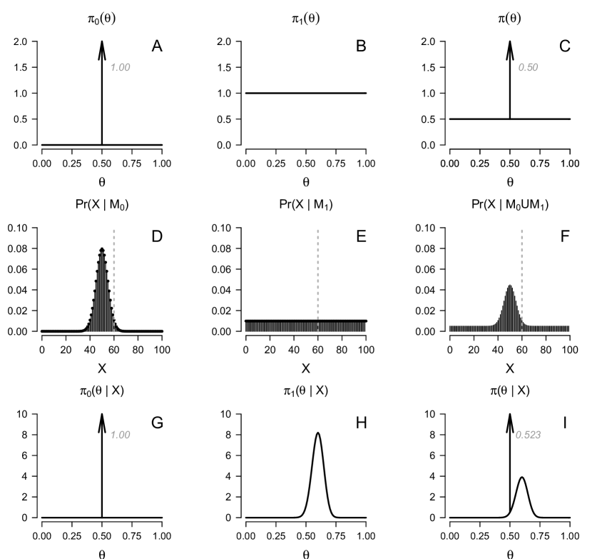
Figure 1: Flipping a possibly biased coin ($X=60$ and $N=100$). The first row shows prior density functions (with the grey numbers next to the arrows corresponding to point mass of the “spike”); middle row shows probability model for the data (with the grey vertical dashed lines corresponding to observed data of $X=60$); and the lower row shows posterior density functions (with the grey numbers next to the arrows corresponding to point mass of the “spike”). Left column corresponds to $M_{0}$, middle column corresponds to $M_{1}$, and right column corresponds to the “mixed/averaged” model.

Each of the two models has a corresponding posterior distribution plotted in panels G and H of Figure 1. If one assumes that $M_{1}$ is the correct model, then the posterior distribution of $\theta$ can be derived analytically (since the Binomial and Beta are conjugate distributions) as:

$$\pi_{1}(\theta|data) =f_{\textrm{Beta}}(\theta,X+\alpha,N-X+\beta)$$

$$=f_{\textrm{Beta}}(\theta,60+1,100-60+1)$$

$$=f_{\textrm{Beta}}(\theta,61,41),$$ (8)

where $f_{\textrm{Beta}}()$ is the Beta probability density function. The posterior mean, $\hat{\theta}_{1}$, posterior median, $\tilde{\theta}_{1}$, and a 95% equal-tailed credible interval, $95\%\textrm{CrI}(\theta)_{1}$, can then be calculated as: $\hat{\theta}_{1}=61/(61+41)=0.598$, $\tilde{\theta}_{1}=0.599$, and $95\%\textrm{CrI}(\theta)_{1}=[0.502,0.691]$. This credible interval, notably, does not include 0.5.

If, alternatively, one assumes that $M_{0}$ is the correct model, then, consequently, the posterior distribution is $\pi_{0}(\theta|data)=\delta_{0.5}(\theta)$. The posterior mean, median, and 95% equal-tailed credible interval will be: $\hat{\theta}_{0}=0.500$, $\tilde{\theta}_{0}=0.500$, and $95\%\textrm{CrI}(\theta)_{0}=[0.500,0.500]$. This credible interval only includes 0.500, indicating total certainty with regards to the true value of $\theta$. As such, it is a very conservative 95% credible interval in the sense that 100% (instead of exactly 95%) of the posterior weight is within the interval.

This coin flip scenario is a good example for illustrating the so-called “incompatibility” discussed by Rouder et al. (2018) and others: The $\textrm{BF}_{10}=0.913$ indicates that the data are more likely to occur under the null, while $95\%\textrm{CrI}(\theta)_{1}=[0.502,0.691]$ excludes 0.500. However, there is no reason to expect that the $\textrm{BF}_{10}$ and $95\%\textrm{CrI}(\theta)_{1}$ will be congruent. If someone decides that $M_{0}$ (‘the coin is fair’) is more likely because $\textrm{BF}_{10}<1$, necessarily their implied prior model odds must be 1:1. However, if they also claim that $\text{Pr}(\theta\in 95\%\textrm{CrI}(\theta)_{1}|data)=0.95$, then they must also believe that $\textrm{Pr}(M_{1})=1$ and $\textrm{Pr}(M_{0})=0$ which is clearly incompatible with the implications made for testing. To be clear, testing and estimation will only be congruent if the (implied) prior model odds adopted for both are the same. In the next section, we review two different ways this can be achieved.

3 Two equivalent approaches

If someone assumes that $M_{1}$ is the correct model (and therefore reports $95\%\textrm{CrI}(\theta)_{1}$), then there is really no sense for them to compute a Bayes factor (or the posterior odds), since the (implied) prior odds are definitive with respect to which of the two models is “correct.” van Ravenzwaaij & Wagenmakers (2021) explain as follows: If one assumes that $M_{1}$ is the correct model, then the null model is “deemed false from the outset, and hence no amount of data can either support or undercut it”.

Alternatively, if someone is uncertain about which of the two models is correct, estimates and credible intervals for $\theta$ should take this uncertainty into account. This can be achieved by either (1) Bayesian model averaging (BMA), or by (2) defining a single “mixture” prior. Both approaches, as we will demonstrate, will deliver the very same results.

Under the BMA approach, one averages the posterior distributions under each of the two models, $\pi_{0}(\theta|data)$ and $\pi_{1}(\theta|data)$, weighted by their relative posterior model probabilities, to obtain an appropriate “averaged” posterior distribution:

$$\pi_{BMA}(\theta|data)= \textrm{Pr}(M_{0}|data)\pi_{0}(\theta|data)+\textrm{Pr}(M_{1}|data)\pi_{1}(\theta|data).$$ (9)

Alternatively, under the single “mixture” prior approach, one defines a single model with a single “mixture” prior, $\pi_{mix}(\theta)$, defined as a weighted combination of $\pi_{0}(\theta)$ and $\pi_{1}(\theta)$ such that:

$$\pi_{mix}(\theta)=\textrm{Pr}(M_{0})\pi_{0}(\theta)+\textrm{Pr}(M_{1})\pi_{1}(\theta).$$

In this case, the corresponding posterior, $\pi_{mix}(\theta|data)$, can also be written as a weighted combination such that:

$$\pi_{mix}(\theta|data) \propto\Big{(}\textrm{Pr}(M_{0})\pi_{0}(\theta)+\textrm{Pr}(M_{1})\pi_{1}(\theta)\Big{)}\times\textrm{Pr}(data|\theta).$$ (10)

The $\pi_{mix}(\theta|data)$ posterior and the $\pi_{BMA}(\theta|data)$ posterior are in fact identical since:

$$\pi_{mix}(\theta|data) \propto\textrm{Pr}(M_{0})\pi_{0}(\theta)\textrm{Pr}(data|\theta)+\textrm{Pr}(M_{1})\pi_{1}(\theta)\textrm{Pr}(data|\theta)$$

$$\propto m_{0}\textrm{Pr}(M_{0})\frac{\pi_{0}(\theta)\textrm{Pr}(data|\theta)}{m_{0}}+m_{1}\textrm{Pr}(M_{1})\frac{\pi_{1}(\theta)\textrm{Pr}(data|\theta)}{m_{1}},$$

$$\propto\frac{m_{0}\textrm{Pr}(M_{0})\pi_{0}(\theta|data)+m_{1}\textrm{Pr}(M_{1})\pi_{1}(\theta|data)}{m_{0}\textrm{Pr}(M_{0})+m_{1}\textrm{Pr}(M_{1})}$$

$$\propto m_{0}\textrm{Pr}(M_{0})\pi_{0}(\theta|data)+m_{1}\textrm{Pr}(M_{1})\pi_{1}(\theta|data)$$

$$\propto\textrm{Pr}(M_{0}|data)\pi_{0}(\theta|data)+\textrm{Pr}(M_{1}|data)\pi_{1}(\theta|data)$$

$$\propto\pi_{BMA}(\theta|data),$$ (11)

where $m_{i}=\textrm{Pr}(data|M_{i})$, for $i=0,1$. Thus, because densities are normalized to integrate to 1, we have that $\pi_{mix}(\theta|data)=\pi_{BMA}(\theta|data)$. As such, point estimates and credible intervals obtained with the BMA approach will be identical to those obtained with the single “mixture” prior approach.

This equality is not always acknowledged in the literature. For example, in describing a mixture model for Bayesian meta-analysis, Röver et al. (2019) do note that the two approaches are equal (“the mixture prior effectively results in a model-averaging approach”), while Gronau et al. (2021) and Bartoš et al. (2021) in proposing a similar approach for Bayesian meta-analysis, do not point out that the BMA approach is exactly equivalent to the single “mixture” prior approach.

Going forward we write simply $\pi(\theta|data)$ instead of using the $\pi_{mix}(\theta|data)$ or $\pi_{BMA}(\theta|data)$ notation, and use $\pi(\theta)$ to denote the “mixed”/”averaged” prior instead of $\pi_{mix}(\theta)$ or $\pi_{BMA}(\theta)$. In our example of the possibly biased coin, with the BMA approach, we obtain, from equation (9):

$$\pi(\theta|data)= 0.523\times\delta_{0.5}(\theta)+0.477\times f_{\textrm{Beta}}(\theta,61,41).$$

Obtaining MCMC draws from this posterior is simple: With 1 million draws from $\pi_{0}(\theta|data)$ and another 1 million draws from $\pi_{1}(\theta|data)$, one can obtain 1 million draws from $\pi(\theta|data)$ by combining together approximately 523 thousand draws from $\pi_{0}(\theta|data)$ with 477 thousand draws from $\pi_{1}(\theta|data)$. See panel I of Figure 1 where the $\pi(\theta|data)$ function is plotted. From these combined draws, we can then compute the posterior mean, $\hat{\theta}$, the posterior median, $\tilde{\theta}$, and the 95% equal-tailed credible interval, $95\%\textrm{CrI}(\theta)$, as: $\hat{\theta}=0.547$, $\tilde{\theta}=0.500$, and $95\%\textrm{CrI}(\theta)=[0.500,0.676]$. Note that the 95% equal-tailed credible interval includes 0.5. Also, note that due to the discontinuity in the posterior, this is a conservative credible interval and is not actually equal-tailed: The [0.500, 0.676] interval includes 96.39% of the posterior weight, since $\textrm{Pr}(\theta<0.500|data)=0.011$ and $\textrm{Pr}(\theta>0.676|data)=0.025$.

Estimation based on $\pi(\theta|data)$ will be entirely congruent with testing based on the posterior model odds, $\textrm{PO}_{10}$, (or the Bayes factor, $\textrm{BF}_{10}$) since both estimation and testing are done using the very same (implied) prior model odds. One could also calculate all of these numbers analytically. For the posterior mean, we calculate:

$$\hat{\theta}= \quad\textrm{Pr}(M_{0}|data)\hat{\theta}_{0}+\textrm{Pr}(M_{1}|data)\hat{\theta}_{1}$$

$$= \quad 0.523\times 0.500+0.477\times 0.598$$

$$= \quad 0.547.$$ (12)

For the 95% equal-tailed credible interval, we calculate $95\%\textrm{CrI}(\theta)=\Big{[}Q_{\theta|data}(0.025),Q_{\theta|data}(0.975)\Big{]}$, where:

$$Q_{\theta|data}(q)=\begin{cases}&\quad Q_{\theta|data,M_{1}}\Big{(}\frac{q}{\textrm{Pr}(M_{1}|data)}\Big{)},\quad\quad\textrm{if}\quad\Big{(}\textrm{Pr}({\theta}<\theta_{0}|data,M_{1})\textrm{Pr}(M_{1}|data)\Big{)}>q,\\ &\quad Q_{\theta|data,M_{1}}\Big{(}1-\frac{1-q}{\textrm{Pr}(M_{1}|data)}\Big{)},\textrm{ if }\Big{(}\textrm{Pr}({\theta}<\theta_{0}|data,M_{1})\textrm{Pr}(M_{1}|data)+\textrm{Pr}(M_{0}|data)\Big{)}<q,\\ &\quad\theta_{0},\quad\quad\quad\quad\quad\quad\quad\quad\quad\quad\quad\textrm{otherwise,}\end{cases}$$ (13)

where $Q_{Z}(q)$, is $q$-th quantile of $Z$, and $\theta_{0}=0.5$. Finally, for the posterior median, we calculate $\tilde{\theta}=Q_{\theta|data}(0.5)=0.500$.

When $\theta_{0}$ is on the boundary of the 95% credible interval, the $\Big{[}Q_{\theta|data}(0.025),Q_{\theta|data}(0.975)\Big{]}$ interval will necessarily be conservative (and not equal-tailed) in the sense that either $\textrm{Pr}(\theta<Q_{\theta|data}(0.025)|data)>0.025$ or $\textrm{Pr}(\theta>Q_{\theta|data}(0.975)|data)>0.025$ and therefore the interval will include more than 95% of the posterior weight. See Campbell & Gustafson (2022) for a discussion on this point.

With the single “mixture” prior approach, from equation (10), we obtain:

$$\pi(\theta|data) \propto 0.5\times f_{Binom}(X,N,\theta)\times\Big{(}\delta_{0.5}(\theta)+1_{\{(0,1)\}}(\theta)\Big{)},$$

where $1_{\{(0,1)\}}(\theta)$ is an indicator function equal to 1 if $\theta\in(0,1)$ and equal to 0 otherwise, as in equation (5). One might recognize this as a version of the well-known “spike-and-slab” model (see van den Bergh et al. (2021)) and Monte Carlo sampling directly from this posterior can be challenging when using popular MCMC software such as JAGS and stan. An easy workaround is to introduce a latent parameter, $\omega$, such that the “mixed prior” is defined in a hierarchical way as follows:

$$\pi(\theta|\omega) =(1-\omega)\pi_{0}(\theta)+\omega\pi_{1}(\theta),$$

$$\omega \sim\textrm{Bernoulli}(\textrm{Pr}(M_{1})).$$

This hierarchical strategy is often referred to as the “product space method”; see Carlin & Chib (1995) and more recently Lodewyckx et al. (2011). See also the discussion about testing as mixture estimation in Robert (2016) and the discussion about unification via the spike-and-slab model in Rouder et al. (2018).

Employing the “product space method” we obtain (using JAGS) 1 million draws from $\pi(\theta|data)$ and can calculate the posterior mean, $\hat{\theta}$, the posterior median, $\tilde{\theta}$, and the 95% equal-tailed credible interval, $95\%\textrm{CrI}(\theta)$, as: $\hat{\theta}=0.547$, $\tilde{\theta}=0.500$, and $95\%\textrm{CrI}(\theta)=[0.500,0.676]$. These numbers are identical to those obtained using the BMA approach.

The “product space method” is also advantageous since $\hat{\omega}$, the posterior mean of $\omega$, is the posterior probability of $M_{1}$. As such, calculation of the posterior odds and of the Bayes factor is straightforward:

$${\textrm{PO}}_{10}=\frac{\textrm{Pr}(M_{1}|data)}{\textrm{Pr}(M_{0}|data)}=\frac{\hat{\omega}}{1-\hat{\omega}},$$

and:

$${\textrm{BF}}_{10}=\left(\frac{\hat{\omega}}{1-\hat{\omega}}\right)/\left(\frac{\textrm{Pr}(M_{1})}{\textrm{Pr}(M_{0})}\right).$$

For the possibly biased coin example, we obtain $\hat{\omega}=0.477$, ${\textrm{PO}}_{10}=0.913$, and ${\textrm{BF}}_{10}=0.913$. These numbers are equal the values calculated analytically in equations (6) and (7).

When the probability of $M_{0}$ given the data is non-negligible, ignoring the $M_{0}$ model “paints an overly optimistic picture of what values $\theta$ is likely to have” (Wagenmakers et al. 2022). As such, there can be a substantial difference between the estimates obtained from the posterior under $M_{1}$ and estimates from the “mixture”/“averaged” posterior. In our example of the possibly biased coin, there is modest evidence in favour of $M_{0}$ with $\textrm{Pr}(M_{0}|data)=0.523$, and as such there is a notable difference between $\hat{\theta}_{1}=0.598$ and $\hat{\theta}=0.547$, and between $95\%\textrm{CrI}(\theta)_{1}=[0.502,0.691]$ and $95\%\textrm{CrI}(\theta)=[0.500,0.676]$.

4 Observing a single coin flip

Wagenmakers et al. (2020) consider the coin flip example but with only a single flip (i.e., with $N=1$) which lands tails (i.e., with $X=0$). In this simple, yet surprisingly interesting scenario, we have, from equation (1):

$$\textrm{Pr}(data|M_{0})=f_{Binom}(0,1,0.5)=0.500,$$

and

$$\textrm{Pr}(data|M_{1})=\int_{t=0}^{t=1}f_{Binom}(0,1,t)dt=0.500.$$

The ratio of these two numbers is equal to the Bayes factor:

$$\textrm{BF}_{10} =\frac{\textrm{Pr}(data|M_{1})}{\textrm{Pr}(data|M_{0})}=\frac{0.500}{0.500}=1,$$

indicating that the single coin flip is “perfectly uninformative” (Wagenmakers et al. 2020) with regards to determining whether the data support $M_{1}$ over $M_{0}$ or vice-versa.

Wagenmakers et al. (2020) do not explicitly define any prior model odds for this example, but do consider $\pi_{J}(\theta)$, a Beta(0.5,0.5) prior on $\theta$, for estimation. Using this prior, a 95% credible interval for $\theta$ is calculated as $95\%\textrm{CrI}(\theta)_{J}=[0.23,1.00]$, and a 66% credible interval for $\theta$ is calculated as $66\%\textrm{CrI}(\theta)_{J}=[0.70,1.00]$. Wagenmakers et al. (2020) then explain their results as follows: “It appears paradoxical that data can be perfectly uninformative for comparing [$M_{0}$ to $M_{1}$ …], and at the same time provide reason to believe that $\theta>0.5$ rather than $\theta<0.5$.”

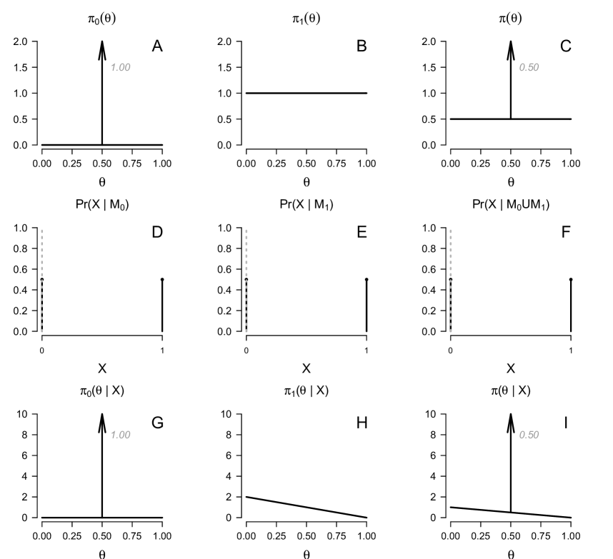
Figure 2: Observing a single coin flip ($X=0$ and $N=1$). The first row shows prior density functions (with the grey numbers next to the arrows corresponding to point mass of the “spike”); middle row shows probability model for the data (with the grey vertical dashed lines corresponding to observed data of $X=60$); and the lower row shows posterior density functions (with the grey numbers next to the arrows corresponding to point mass of the “spike”). Left column corresponds to $M_{0}$, middle column corresponds to $M_{1}$, and right column corresponds to the “mixed/averaged” model.

As was the case with $N=100$ coin flips, the “paradox” here is simply due to the fact that different implied prior model odds are being used for testing and for estimation. If I have “reason to believe” that $\textrm{Pr}(\theta\in[0.70,1.00]|data)=0.66$, then necessarily, I could not have believed, prior to flipping the coin, that either $M_{0}$ or $M_{1}$ were the true data generating mechanism. This is because a belief that $\textrm{Pr}(\theta\in[0.70,1.00]|data)=0.66$ necessarily implies a corresponding a priori belief in the $\pi_{J}(\theta)$ prior.

For someone who believes in the $\pi_{J}(\theta)$ prior, the above Bayes factor, $\textrm{BF}_{10}$, regardless of it’s value, is meaningless since both $\textrm{Pr}(M_{0})=0$ and $\textrm{Pr}(M_{1})=0$. The prior model odds will be ill-defined (i.e., $\textrm{PO}_{10}=$0:0) and therefore posterior model odds cannot be determined regardless of the observed data. To be clear, the Bayes factor is only meaningful to someone if they are willing to consider that both models, $M_{0}$ and $M_{1}$, are a priori, plausible.

Notably, if one assumes prior model odds of 1:1 (such that $\textrm{Pr}(M_{0})=\textrm{Pr}(M_{1})=0.5$), estimation based on the “mixture”/“averaged” posterior will be entirely congruent with the “perfectly uninformative” $\textrm{BF}_{10}=1$. Indeed, we obtain $95\%\textrm{CrI}(\theta)=[0.025,0.776]$ and a conservative $66\%\textrm{CrI}(\theta)=[0.188,0.500]$, which suggests that even a single flip is informative with regards to inferring $\theta$. However, we also obtain:

$$\textrm{Pr}(M_{0}|data)=\frac{0.5}{0.5+1\times 0.5}=0.500,$$

$$\textrm{Pr}(M_{1}|data)=\frac{1\times 0.5}{0.5+1\times 0.5}=0.500,\quad$$

and

$$\textrm{PO}_{10} =\frac{0.5}{0.5}\times 1=1.000,$$

which suggests that, while we have gained some information about $\theta$, $M_{0}$ and $M_{1}$ remain equally likely to be the true model. When framed in this manner, there is nothing paradoxical: Conclusions about $\theta$ and conclusions about $M_{0}$ vs. $M_{1}$ are entirely congruent since both are based on the same prior model odds. Figure 2 plots the “mixture”/“averaged” posterior where we see that, notably, exactly 50% of posterior mass for $\theta$ is at exactly $\theta=0.500$. Looking at the area under the curve, one can also determine that $\textrm{Pr}(\theta\neq 0.5)=\textrm{Pr}(\theta<0.5)+\textrm{Pr}(\theta>0.5)=0.375+0.125=0.5$.

Using the “mixture”/“averaged” posterior for estimation (with the same prior model odds that are used for testing) will ensure that there is no “incompatibility” or “mismatch” between testing models and estimating $\theta$. We emphasize that this applies universally, regardless of how $M_{0}$ and $M_{1}$ are defined. Notably, some researchers have claimed that the “incompatibility” problem only occurs when considering point-null hypotheses (e.g., Tendeiro & Kiers (2019) write that: “The problem is directly related to the use of the point null model”). In the next section, we consider an example that does not involve a point null.

5 With an interval null model

Instead of questioning whether or not the coin is exactly fair, suppose one wishes to determine whether or not the coin is fair within some negligible margin. Indeed, it could be argued that there is no such thing as a perfectly fair coin (Diaconis et al. 2007) and that bias is only consequential if it is of a certain non-negligible magnitude.

In other words, one might argue that $\theta$ will never be exactly equal to 0.5, and therefore consider “non-overlapping hypotheses” (Morey & Rouder 2011) with priors for two competing models, $M_{2}$ and $M_{3}$, defined by partitioning a Uniform(0,1) density function as follows:

$$\pi_{2}(\theta)=\begin{cases}10,&\text{if }\theta\in\Theta_{0}\\ 0,&\text{otherwise,}\end{cases}$$

and

$$\pi_{3}(\theta)=\begin{cases}1/0.9,&\text{if }\theta\in\Theta_{1}\\ 0,&\text{otherwise.}\end{cases}$$

where $\Theta_{0}=[0.45,0.55]$ and $\Theta_{1}=(0,0.45)\cup(0.55,1)$; see panels A and B of Figure 3. The corresponding posterior distributions (see panels G and H of Figure 3) are:

$$\pi_{2}(\theta|data) \propto f_{\textrm{Beta}}(\theta,X+1,N-X+1)\times 10\times 1_{\{\Theta_{0}\}}(\theta).$$

and

$$\pi_{3}(\theta|data) \propto f_{\textrm{Beta}}(\theta,X+1,N-X+1)\times 1.11\times 1_{\{\Theta_{1}\}}(\theta).$$

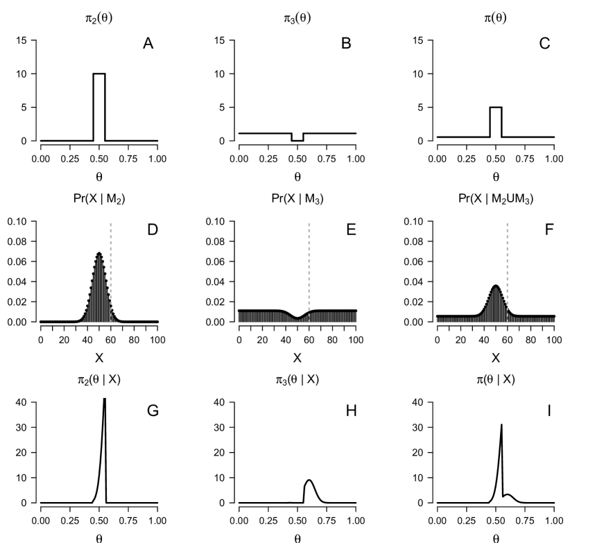
Figure 3: Observing a 100 coin flips ($X=60$ and $N=100$) with “non-overlapping hypotheses”. The first row shows prior density functions; middle row shows probability model for the data (with the grey vertical dashed lines corresponding to observed data of $X=60$); and lower row shows posterior density functions. Left column corresponds to $M_{2}$, middle column corresponds to $M_{3}$, and right column corresponds to the “mixed/averaged” model.

Having observed $X=60$ “heads” out of $N=100$ coin flips, we calculate from equation (1) (see panels D and E of Figure 3):

$$\textrm{Pr}(data|M_{2})=\int_{t=0.45}^{t=0.55}10\times f_{Binom}(60,100,t)dt=0.016,$$

$$\textrm{Pr}(data|M_{3})=\frac{1}{0.9}\left(\int_{t=0}^{t=0.45}f_{Binom}(60,100,t)dt+\int_{t=0.55}^{t=1}f_{Binom}(60,100,t)dt\right)=0.009.$$

and

$$\textrm{BF}_{32} =\frac{\textrm{Pr}(data|M_{3})}{\textrm{Pr}(data|M_{2})}=\frac{0.009}{0.016}=0.584.$$

For estimation, suppose one assumes a $\textrm{Uniform}(0,1)$ prior (i.e., the $\pi_{1}(\theta)$ prior as defined in equation (5)), so as to give equal prior weight to all values between 0 and 1. From the corresponding $\pi_{1}(\theta|data)$ posterior (see equation (2)), one obtains a posterior mean of $\hat{\theta}_{1}=0.598$, a posterior median of $\tilde{\theta}_{1}=0.599$, and $95\%\textrm{CrI}(\theta)_{1}=[0.502,0.691]$. One can also calculate $\textrm{Pr}_{1}(\theta\in\Theta_{1}|data)=0.840$.

This is therefore another example of the so-called “mismatch” between Bayesian testing and posterior estimation: The $\textrm{BF}_{32}=0.584$ appears to support the null, while $95\%\textrm{CrI}(\theta)_{1}=[0.502,0.691]$ excludes 0.500. As was the case in the previous examples with the point-null hypothesis, the “mismatch” here is due to different implied prior model odds being used for testing and for estimation.

As established by Liao et al. (2021), the implied prior model odds that correspond to estimation with the Uniform(0,1) prior (i.e., under the $\pi_{1}(\theta|data)$ posterior) can be calculated as:

$$\textrm{IPMO}_{1}=\frac{\textrm{Pr}_{1}(\theta\in\Theta_{1})}{\textrm{Pr}_{1}(\theta\in\Theta_{0})}=9:1,$$

where

$$\textrm{Pr}_{1}(\theta\in\Theta_{1})=\int_{\Theta_{1}}\pi_{1}(\theta)d\theta=\int_{t=0}^{t=0.45}1dt+\int_{t=0.55}^{t=1}1dt=0.90.$$

and

$$\textrm{Pr}_{1}(\theta\in\Theta_{0})=\int_{\Theta_{0}}\pi_{1}(\theta)d\theta=\int_{t=0.45}^{t=0.55}1dt=0.10.$$

Notably, by multiplying these implied prior model odds by the Bayes factor, one obtains posterior odds that favour $M_{3}$ and which are entirely congruent with the $\pi_{1}(\theta|data)$ posterior:

$$\textrm{IPMO}_{1}\times\textrm{BF}_{32}=9\times 0.584=5.255=\frac{\textrm{Pr}_{1}(\theta\in\Theta_{1}|data)}{\textrm{Pr}_{1}(\theta\in\Theta_{0}|data)}=\frac{0.840}{0.160}.$$

Alternatively, if one assumes equal prior model odds (i.e., assumes a priori that $\textrm{Pr}(M_{2})=\textrm{Pr}(M_{3})=0.5$), then the posterior odds favour $M_{2}$:

$$\textrm{PO}_{32}=\frac{\textrm{Pr}(M_{3})}{\textrm{Pr}(M_{2})}\times\textrm{BF}_{32}=\frac{0.5}{0.5}\times 0.584=0.584$$

Estimation that is congruent with $\textrm{PO}_{32}=0.584$ can be done by invoking the “mixed/averaged” prior:

$${\pi}(\theta) =\textrm{Pr}(M_{2})\pi_{2}(\theta)+\textrm{Pr}(M_{3})\pi_{3}(\theta),$$

$$=0.5\times\frac{1}{0.1}\times 1_{\{\Theta_{0}\}}(\theta)+0.5\times\frac{1}{0.9}\times 1_{\{\Theta_{1}\}}(\theta)$$

and the corresponding “mixed/averaged” posterior:

$$\pi(\theta|data) \propto\textrm{Pr}(M_{2}|data)\pi_{2}(\theta|data)+\textrm{Pr}(M_{3}|data)\pi_{3}(\theta|data)$$

$$\propto 0.631\times f_{\textrm{Beta}}(\theta,X+1,N-X+1)\times 10\times 1_{\{\Theta_{0}\}}(\theta)\quad+$$

$$\quad\quad\quad\quad 0.369\times f_{\textrm{Beta}}(\theta,X+1,N-X+1)\times 1.11\times 1_{\{\Theta_{1}\}}(\theta).$$

From the $\pi(\theta|data)$ posterior, one obtains a posterior mean of $\hat{\theta}=0.557$, a posterior median of $\tilde{\theta}=0.543$, and $95\%\textrm{CrI}(\theta)=[0.479,0.673]$.

To reiterate, testing and estimation will only be congruent if the (implied) prior model odds adopted for both are the same. In this example, when estimation is based on a Uniform(0,1) prior for $\theta$, the implied prior model odds are 9:1, whereas when testing decisions about which model is most likely to be true are based on whether or not $\textrm{BF}_{32}>1$, the implied prior model odds are 1:1. As such, it is no surprise that the two approaches provide different answers.

6 A difference in personality types?

As an example from applied research, consider Heck et al. (2022) who present the analysis of data concerning the difference between type D personality and non-type D personality for two outcome variables: BMI (body mass index) and NAS (negative affectivity score). See summary data in Table 1 and note that these data were originally analyzed by Lin et al. (2019).

Heck et al. (2022) consider two competing models, a null model, $M_{0}$, which corresponds to the lack of an association between personality type and outcome, and an alternative model, $M_{1}$, which suggests the existence of an association. Let $\theta$ be the parameter of interest, the standardized effect size. The difference in personality types is associated with an increase of $\theta$ standard deviations in the outcome variable and a Normal model for the data is defined as:

$$\textrm{Pr}(data|\theta,\sigma^{2})=\prod_{i=1}^{n}f_{Normal}\left(Y_{i},\mu+X_{i}\times\frac{\sigma\theta}{2},\sigma^{2}\right),$$

where $f_{Normal}()$ is the Normal probability density function, $Y_{i}$ is the continuous outcome variable for the $i$-th observation (i.e., $Y_{i}$ is the $i$-th subject’s BMI score in the first analysis, and the $i$-th subject’s NAS score in the second analysis), and $X_{i}$ corresponds to the $i$-th subject’s personality type such that $X_{i}=-1$ indicates a non-type D personality and $X_{i}=1$ indicates a type D personality.

We have three parameters, $\mu$, $\theta$ and $\sigma^{2}$ for which we must define priors and we define these priors for both $M_{0}$ and $M_{1}$ as:

$$\pi_{0}(\mu)=1,\quad\pi_{0}(\sigma^{2})=\frac{1}{\sigma^{2}},\quad\pi_{0}(\theta)=\delta_{0}(\theta),\quad$$

and

$$\pi_{1}(\mu)=1,\quad\pi_{1}(\sigma^{2})=\frac{1}{\sigma^{2}},\quad\pi_{1}(\theta)=f_{\textrm{Cauchy}}(\theta,0.707),\quad$$

where, for both $M_{0}$ and $M_{1}$, noninformative Jeffreys priors are defined for $\sigma^{2}$, and for $\mu$; and $f_{\textrm{Cauchy}}(x,s)=((s\pi)(1+(x/s)^{2}))^{-1}$ is the Cauchy probability density function evaluated at $x$, with scale parameter $s$. Specifying noninformative Jeffreys’ priors is mathematically convenient for calculating the Bayes factor. However, these improper priors cannot be accurately specified in popular MCMC sofware such as WinBugs, JAGS, and greta; see Faulkenberry (2018).

For the BMI outcome, Heck et al. (2022) report a Bayes factor of $\textrm{BF}_{10}=1/4.2$ and sample from the posterior $\pi_{1}(\theta|data)$ (thereby implicitly assuming $M_{1}$ is correct) to obtain a posterior median of $\tilde{\theta}_{1}=0.05$, and $95\%\textrm{CrI}(\theta)_{1}=[-0.35,0.45]$. The posterior mean (not reported) is $\hat{\theta}_{1}=0.05$.

Assuming equal a priori model probabilities, we can calculate from equation (2):

$$\textrm{Pr}(M_{0}|data)\quad= \quad\frac{\textrm{Pr}(M_{0})}{(BF_{10}\times\textrm{Pr}(M_{1})+\textrm{Pr}(M_{0}))}$$

$$= \quad\frac{0.5}{0.5/4.2+0.5}$$

$$= \quad\frac{0.5}{0.5/4.2+0.5}$$

$$= \quad 0.808,$$

indicating considerable evidence in favour of the null model.

Under $M_{0}$, we have $\theta=0$. Therefore, we can obtain a Monte Carlo sample from the “mixture”/“averaged” posterior, $\pi(\theta|data)$, by simply combining 192 thousand draws for $\theta$ from $\pi_{1}(\theta|data)$ with 808 thousand zeros. From this “combined” sample we calculate $\tilde{\theta}=0.00$, $\hat{\theta}=0.01$, and $95\%\textrm{CrI}(\theta)=[-0.18,0.28]$. One can also obtain these estimates using equation (13) with $\theta_{0}=0$. These numbers are notably different than those based on the $\pi_{1}(\theta|data)$ posterior reported by Heck et al. (2022).

For the NAS outcome, Heck et al. (2022) report a Bayes factor of $\textrm{BF}_{10}=10^{20}$ and sample from the posterior $\pi_{1}(\theta|data)$ (implicitly assuming $M_{1}$ is correct) to obtain a posterior median of $\tilde{\theta}_{1}=-2.36$, and $95\%\textrm{CrI}(\theta)_{1}=[-2.85,-1.87]$. The posterior mean (not reported) is $\hat{\theta}_{1}=-2.36$. The evidence in favour of $M_{1}$ is overwhelming, $\textrm{Pr}(M_{1}|data)>0.99$, and therefore estimates from the “mixture”/“averaged” posterior (obtained using either the BMA approach or the “mixture” prior approach) are nearly identical: $\tilde{\theta}=-2.36$, $\hat{\theta}=-2.36$, and $95\%\textrm{CrI}(\theta)=[-2.85,-1.87]$.

Outcome	Non-Type D ($n=193$)	Type D ($n=23$)
BMI	$\bar{X}=26.0$ (SD=4.9)	$\bar{X}=25.7$ (SD=4.4)
NAS	$\bar{X}=5.5$ (SD=4.2)	$\bar{X}=15.4$ (SD=3.5)

Table 1: The sample mean, $\bar{X}$, and sample standard deviation, $SD$, for each of the two groups (type D personality and non-type D personality) and each of the two outcome variables (BMI (body mass index) and NAS (negative affectivity score)). The data were originally analyzed by Lin et al. (2019).

7 Flipping one million coins

To better explain why we believe researchers should report estimates from the “mixture”/“averaged” posterior instead of estimates from $\pi_{1}(\theta|data)$ or other posteriors, we return one final time to the coin flip example, but this time with $N=10$ flips. Let us explicitly assume that $M_{0}$ and $M_{1}$ are a priori equally likely: $\textrm{Pr}(M_{0})=\textrm{Pr}(M_{1})=0.5$.

Consider the following thought experiment. By drawing from the “mixture”/“averaged” prior, $\pi(\theta)$, one obtains a coin for which $\theta=\theta^{[1]}$. Flipping this coin $N=10$ times generates a total of $X=4$ “heads” and the posterior mean, under $M_{1}$, is:

$$\hat{\theta}_{1} =(X+\alpha)/(N+\alpha+\beta)$$

$$=(4+1)/(10+1+1)$$

$$=\frac{5}{12}=0.417.$$ (14)

The equal-tailed 95% credible interval is $95\%\textrm{CrI}(\theta)_{1}=[0.167,0.692]$. From equation (12), the posterior mean, taking into account the model uncertainty, is:

$$\hat{\theta} =\textrm{Pr}(M_{0}|data)\hat{\theta}_{0}+\textrm{Pr}(M_{1}|data)\hat{\theta}_{1}$$

$$=0.693\times 0.5+0.307\times 0.417$$

$$=0.474,$$ (15)

and the equal-tailed 95% credible interval is $95\%\textrm{CrI}(\theta)=[0.227,0.616]$.

Now suppose we obtain a second coin from the “mixed”/“averaged” prior for which $\theta=\theta^{[2]}$. Flipping this second coin $N=10$ times generates a total of $X=8$ “heads”. Then the posterior mean, under $M_{1}$, is $\hat{\theta}_{1}=\frac{9}{12}=0.750$, and the equal-tailed 95% credible interval is $95\%\textrm{CrI}(\theta)_{1}=[0.482,0.940]$. The posterior mean, taking into account the model uncertainty, is $\hat{\theta}=0.669$, and the equal-tailed 95% credible interval is $95\%\textrm{CrI}(\theta)=[0.500,0.930]$. Note that due to the discontinuity in the posterior, this is a conservative 95% credible interval that is not actually equal-tailed: The [0.500, 0.930] interval includes 95.29% of the posterior weight, since $\textrm{Pr}(\theta<0.500|data)=0.022$ and $\textrm{Pr}(\theta>0.930|data)=0.025$.

We implemented this process by simulation again and again obtaining 1 million coins from the “mixed”/“averaged” prior (i.e., generating 1 million values $\theta^{[1]},\ldots,\theta^{[1000000]}$ from $\pi(\theta)$), and flipping each of these coins 10 times; see Table 2. In total, we obtained a total of 148,022 coins for which $X=4$; see Table 3.

Because this is a simulation, it is possible to reveal the underlying true values of $\theta^{[1]},\ldots,\theta^{[1000000]}$. For the subset of coins for which $X=4$, the average of these values is 0.474. For lack of better notation we write $\textrm{E}(\theta^{[j]}|X^{[j]}=4)=0.474$. Notably, this equals $\hat{\theta}$ when $X=4$ (see equation (15)), but does not equal $\hat{\theta}_{1}$ when $X=4$ (see equation (14)). Nor does it equal $\frac{4}{10}$. In this sense, both $\hat{\theta}_{1}$ and $\frac{X}{N}$ overestimate $\theta$, when $X=4$. Table 3 shows these comparisons for $X=0,...,10$.

Furthermore, amongst the 148,022 simulated $\theta^{[j]}$ values for which $X=4$, exactly 140,459 are within the interval of $95\%\textrm{CrI}(\theta)$=[0.227,0.616]. Notably, this proportion is 140,459/148,022 = 0.95. In comparison, the proportion of the 148,022 values within the interval of $95\%\textrm{CrI}(\theta)_{1}$=[0.167, 0.692] is 0.98. Again, for lack of better notation, we write $\textrm{Pr}\Big{(}\theta^{[j]}\in 95\%\textrm{CrI}(\theta)_{1}\Big{|}X^{[j]}=4\Big{)}=0.98$, and $\textrm{Pr}\Big{(}\theta^{[j]}\in 95\%\textrm{CrI}(\theta)\Big{|}X^{[j]}=4\Big{)}=0.95$. In this sense, the $95\%\textrm{CrI}(\theta)_{1}$ interval is too wide, whereas the $95\%\textrm{CrI}(\theta)$ is appropriately wide. Table 4 shows these comparisons for $X=0,...,10$.

$j$	$\theta^{[j]}$	$X^{[j]}$	$N$	$\hat{\theta}_{1}$	$95\%\textrm{CrI}(\theta)_{1}$	$\hat{\theta}$	$95\%\textrm{CrI}(\theta)$
1	0.50	4	10	0.417	[0.167,0.692]	0.474	[0.227, 0.616]
2	0.77	8	10	0.750	[0.482, 0.940]	0.669	[0.500, 0.930]
3	0.91	8	10	0.750	[0.482, 0.940]	0.669	[0.500, 0.930]
4	0.11	2	10	0.250	[0.060, 0.518]	0.331	[0.070, 0.500]
5	0.87	9	10	0.833	[0.587, 0.977]	0.801	[0.500, 0.976]
6	0.50	7	10	0.667	[0.390, 0.891]	0.573	[0.445, 0.860]
7	0.50	5	10	0.500	[0.234, 0.766]	0.500	[0.312, 0.688]
8	0.31	1	10	0.167	[0.023, 0.413]	0.199	[0.024, 0.500]
$\vdots$	$\vdots$	$\vdots$	$\vdots$	$\vdots$	$\vdots$	$\vdots$	$\vdots$
$1,000,000$	0.60	6	10	0.583	[0.308, 0.833]	0.526	[0.384, 0.773]

Table 2: One million coins: For the $j$-th coin we observe $X^{[j]}$ “heads” out of $N=10$ flips, we calculate the posterior estimates. Whenever $0.500$ is on the boundary of the $95\%\textrm{CrI}(\theta)$ interval, the interval will be conservative. Specifically, for $X=1$ and $X=9$, 96.97% of the posterior weight will be within the interval; for $X=2$ and $X=8$, 95.29% of the posterior weight will be within the interval.

$x$	# of coins	$\frac{x}{N}$	$\hat{\theta}_{1}$	$\hat{\theta}$	$\textrm{E}(\theta^{[j]}|X^{[j]}=x)$
0	45,864	0.0	0.083	0.088	0.087
1	50,180	0.1	0.167	0.199	0.198
2	67,281	0.2	0.250	0.331	0.331
3	104,309	0.3	0.333	0.427	0.427
4	148,022	0.4	0.417	0.474	0.474
5	168,651	0.5	0.500	0.500	0.500
6	148,502	0.6	0.583	0.526	0.526
7	103,961	0.7	0.667	0.573	0.573
8	67,353	0.8	0.750	0.669	0.670
9	49,939	0.9	0.833	0.801	0.801
10	45,938	1.0	0.917	0.912	0.913

Table 3: Simulation study results: Average values obtained from the subset set of “coins” for which $X=x$ “heads”. For example, among the subset of $104,309$ coins that produced $X=3$, the average of $\theta^{[j]}$ values is $0.427$, a numerical approximation to $\textrm{E}(\theta^{[j]}|X^{[j]}=3)$. Whereas the posterior mean estimate (taking into account the model uncertainty) whenever $X^{[j]}=3$ is $\hat{\theta}=0.427$.

$x$	# of coins	$\textrm{Pr}\Big{(}\theta^{[j]}\in 95\%\textrm{CrI}(\theta)_{1}|X^{[j]}=x\Big{)}$	$\textrm{Pr}\Big{(}\theta^{[j]}\in 95\%\textrm{CrI}(\theta)|X^{[j]}=x\Big{)}$
0	45,864	0.940	0.950
1	50,180	0.858	0.968
2	67,281	0.967	0.953
3	104,309	0.978	0.951
4	148,022	0.984	0.949
5	168,651	0.987	0.951
6	148,502	0.985	0.950
7	103,961	0.978	0.950
8	67,353	0.967	0.955
9	49,939	0.860	0.970
10	45,938	0.938	0.949

Table 4: Simulation study results: Proportion of coins (from the subset for which $X=x$ “heads”) within each credible interval. For example, amongst the 148,502 simulated $\theta^{[j]}$ values for which $X=6$, exactly 95.0% are within the interval of $95\%\textrm{CrI}(\theta)$=[0.384, 0.773]. Note that due to the discontinuity in the posterior, for each of $X=1$, $X=2$, $X=8$, and $X=9$, the $95\%\textrm{CrI}(\theta)$ interval is conservative and therefore we expect to see that more than 95.0% of simulated $\theta^{[j]}$ values are within the interval; see caption of Table 2 for specific values.

The behaviour exhibited in Tables 3 and 4 is completely general mathematically. Generically, let $(\theta^{[j]},X^{[j]})$ be a random draw as is used to construct Table 2, row by row, e.g., $\theta^{[j]}$ is drawn from $\pi(\theta)$, and then $X^{[j]}$ is drawn from “the model” with $\theta$ set equal to $\theta^{[j]}$. Thus the average of $\theta^{[j]}$ when $X=x$ (the last column of Table 3) is simply (a Monte Carlo approximation to) $\textrm{E}(\theta^{[j]}|X^{[j]}=x)$, for each $x$. But since $(\theta^{[j]},X^{[j]})$ is nothing more than a joint draw from the amalgamation of the prior and statistical model, $\textrm{E}(\theta^{[j]}|X^{[j]}=x)$ and $\hat{\theta}$ when $X=x$, are one and the same. By definition then, if we repeatedly sample parameter and data pairs this way, the average of the parameter values amongst draws yielding a specific data value is the posterior mean of the parameter given that data value. The same calibration idea applies to credible intervals so that $\textrm{Pr}\Big{(}\theta^{[j]}\in 95\%\textrm{CrI}(\theta)\Big{|}X^{[j]}=x\Big{)}\geq 0.95$. Note that in the absence of a point mass (i.e., without the “spike”), this will be a strict equality (Campbell & Gustafson 2022).

This strongly supports the argument that when considering model uncertainty via a Bayes factor, $\hat{\theta}$ is the appropriate estimate to report and $95\%\textrm{CrI}(\theta)$ is the appropriate credible interval. While these sorts of calibration properties of Bayesian estimators with respect to repeated sampling of data under different parameter values feature sporadically in the literature (e.g., Rubin & Schenker (1986)), they do not seem to be widely known. They do however, underpin the scheme of Cook et al. (2006) to validate Markov Chain Monte Carlo approximations to posterior quantities and they are also discussed more recently in Gustafson & Greenland (2009). Importantly, we note that this sense of calibration arises only when the prior truly corresponds to the data-generating process.

8 Conclusion

In conclusion, there is no mismatch between the Bayes factor (or the posterior odds) and Bayesian posterior estimation with an appropriately defined prior and posterior. Our recommendation is therefore very simple. If one reports a Bayes factor comparing $M_{0}$ and $M_{1}$, then one should also report posterior estimates based on the “mixed/“averaged” posterior, $\pi(\theta|data)$, with prior model odds appropriately specified. Researchers should refrain from reporting posterior estimates based on $\pi_{1}(\theta|data)$ (which implicitly assumes $M_{1}$ is correct) or estimates based on other posteriors for which the Bayes factor is meaningless. We see no reason why disregarding $M_{0}$ “for the purpose of parameter estimation” (Wagenmakers & Gronau 2020) is advisable.

On a final note, in order to keep things as accessible as possible, all of the examples considered in this paper were univariate inference problems involving only two models. Our conclusions and recommendations, however, also apply to more complex problems. On this point, we refer interested readers to Rossell & Telesca (2017), who consider strategies for how to use the same prior for both estimation and model selection in high-dimensional settings to achieve coherence between estimation and testing, and to Lavine & Schervish (1999) and Oelrich et al. (2020), who discuss Bayes factor based model selection in scenarios involving more than two models.

References

- (1)
- Bartoš et al. (2021) Bartoš, F., Gronau, Q. F., Timmers, B., Otte, W. M., Ly, A. & Wagenmakers, E.-J. (2021), ‘Bayesian model-averaged meta-analysis in medicine’, Statistics in Medicine 40(30), 6743–6761.
- Campbell & Gustafson (2022) Campbell, H. & Gustafson, P. (2022), ‘Defining a credible interval is not always possible with “point-null” priors: A lesser-known consequence of the Jeffreys-Lindley paradox’, arXiv preprint arXiv:2210.00029 .
- Carlin & Chib (1995) Carlin, B. P. & Chib, S. (1995), ‘Bayesian model choice via Markov chain Monte Carlo methods’, Journal of the Royal Statistical Society: Series B (Methodological) 57(3), 473–484.
- Cook et al. (2006) Cook, S. R., Gelman, A. & Rubin, D. B. (2006), ‘Validation of software for Bayesian models using posterior quantiles’, Journal of Computational and Graphical Statistics 15(3), 675–692.
- Diaconis et al. (2007) Diaconis, P., Holmes, S. & Montgomery, R. (2007), ‘Dynamical bias in the coin toss’, SIAM review 49(2), 211–235.
- Faulkenberry (2018) Faulkenberry, T. J. (2018), ‘A tutorial on generalizing the default Bayesian -test via posterior sampling and encompassing priors’, arXiv preprint arXiv:1812.03092 .
- Gelman & Nolan (2002) Gelman, A. & Nolan, D. (2002), ‘You can load a die, but you can’t bias a coin’, The American Statistician 56(4), 308–311.
- Gronau et al. (2021) Gronau, Q. F., Heck, D. W., Berkhout, S. W., Haaf, J. M. & Wagenmakers, E.-J. (2021), ‘A primer on Bayesian model-averaged meta-analysis’, Advances in Methods and Practices in Psychological Science 4(3), doi:10.1177/25152459211031256.
- Gustafson & Greenland (2009) Gustafson, P. & Greenland, S. (2009), ‘Interval estimation for messy observational data’, Statistical Science 24(3), 328–342.
- Heck et al. (2022) Heck, D. W., Boehm, U., Böing-Messing, F., Bürkner, P.-C., Derks, K., Dienes, Z., Fu, Q., Gu, X., Karimova, D., Kiers, H. A. et al. (2022), ‘A review of applications of the Bayes factor in psychological research.’, Psychological Methods (Advance online publication).
- Kelter (2022) Kelter, R. (2022), ‘The evidence interval and the Bayesian evidence value: On a unified theory for Bayesian hypothesis testing and interval estimation’, British Journal of Mathematical and Statistical Psychology 75, 550–592.
- Lavine & Schervish (1999) Lavine, M. & Schervish, M. J. (1999), ‘Bayes factors: What they are and what they are not’, The American Statistician 53(2), 119–122.
- Liao et al. (2021) Liao, J., Midya, V. & Berg, A. (2021), ‘Connecting and contrasting the bayes factor and a modified rope procedure for testing interval null hypotheses’, The American Statistician 75(3), 256–264.
- Lin et al. (2019) Lin, T.-K., You, K.-X., Hsu, C.-T., Li, Y.-D., Lin, C.-L., Weng, C.-Y. & Koo, M. (2019), ‘Negative affectivity and social inhibition are associated with increased cardiac readmission in patients with heart failure: A preliminary observation study’, Plos One 14(4), e0215726.
- Lodewyckx et al. (2011) Lodewyckx, T., Kim, W., Lee, M. D., Tuerlinckx, F., Kuppens, P. & Wagenmakers, E.-J. (2011), ‘A tutorial on Bayes factor estimation with the product space method’, Journal of Mathematical Psychology 55(5), 331–347.
- Morey & Rouder (2011) Morey, R. D. & Rouder, J. N. (2011), ‘Bayes factor approaches for testing interval null hypotheses.’, Psychological Methods 16(4), 406–419.
- Oelrich et al. (2020) Oelrich, O., Ding, S., Magnusson, M., Vehtari, A. & Villani, M. (2020), ‘When are Bayesian model probabilities overconfident?’, arXiv preprint arXiv:2003.04026 .
- O’Hagan & Forster (2004) O’Hagan, A. & Forster, J. J. (2004), Kendall’s advanced theory of statistics, volume 2B: Bayesian inference, 2 edn, Arnold, London.
- Puga et al. (2015a) Puga, J. L., Krzywinski, M. & Altman, N. (2015a), ‘Bayes’ theorem: Incorporate new evidence to update prior information’, Nature Methods 12(4), 277–279.
- Puga et al. (2015b) Puga, J. L., Krzywinski, M. & Altman, N. (2015b), ‘Bayesian statistics: today’s predictions are tomorrow’s priors’, Nature Methods 12(5), 377–379.
- Robert (2016) Robert, C. P. (2016), ‘The expected demise of the Bayes factor’, Journal of Mathematical Psychology 72, 33–37.
- Rossell & Telesca (2017) Rossell, D. & Telesca, D. (2017), ‘Nonlocal priors for high-dimensional estimation’, Journal of the American Statistical Association 112(517), 254–265.
- Rouder et al. (2018) Rouder, J. N., Haaf, J. M. & Vandekerckhove, J. (2018), ‘Bayesian inference for psychology, part IV: Parameter estimation and Bayes factors’, Psychonomic Bulletin & Review 25(1), 102–113.
- Röver et al. (2019) Röver, C., Wandel, S. & Friede, T. (2019), ‘Model averaging for robust extrapolation in evidence synthesis’, Statistics in Medicine 38(4), 674–694.
- Rubin & Schenker (1986) Rubin, D. B. & Schenker, N. (1986), ‘Efficiently simulating the coverage properties of interval estimates’, Journal of the Royal Statistical Society: Series C (Applied Statistics) 35(2), 159–167.
- Tendeiro & Kiers (2019) Tendeiro, J. N. & Kiers, H. A. (2019), ‘A review of issues about null hypothesis bayesian testing.’, Psychological Methods 24(6), 774–795.
- van den Bergh et al. (2021) van den Bergh, D., Haaf, J. M., Ly, A., Rouder, J. N. & Wagenmakers, E.-J. (2021), ‘A cautionary note on estimating effect size’, Advances in Methods and Practices in Psychological Science 4(1), doi:10.1177/2515245921992035.
- van Ravenzwaaij & Wagenmakers (2021) van Ravenzwaaij, D. & Wagenmakers, E.-J. (2021), ‘Advantages masquerading as’ issues’ in Bayesian hypothesis testing: A commentary on Tendeiro and Kiers (2019).’, Psychological Methods 27(3), 451–465.
- Wagenmakers & Gronau (2020) Wagenmakers, E.-J. & Gronau, Q. F. (2020), ‘Overwhelming evidence for vaccine efficacy in the Pfizer trial: An interim Bayesian analysis’, PsyArXiv: 10.31234/osf.io/fs562.
- Wagenmakers et al. (2022) Wagenmakers, E.-J., Gronau, Q. F., Dablander, F. & Etz, A. (2022), ‘The support interval’, Erkenn 87, 589–601.
- Wagenmakers et al. (2020) Wagenmakers, E.-J., Lee, M. D., Rouder, J. N. & Morey, R. D. (2020), The principle of predictive irrelevance or why intervals should not be used for model comparison featuring a point null hypothesis, in C. W. Gruber, ed., ‘The Theory of Statistics in Psychology’, Springer, Cham, Switzerland, pp. 111–129.
- Wagenmakers et al. (2018) Wagenmakers, E.-J., Marsman, M., Jamil, T., Ly, A., Verhagen, J., Love, J., Selker, R., Gronau, Q. F., Šmíra, M., Epskamp, S. et al. (2018), ‘Bayesian inference for psychology. Part I: Theoretical advantages and practical ramifications’, Psychonomic Bulletin & Review 25(1), 35–57.