Evolutionary shift detection with ensemble variable selection

1. Abrupt environmental changes can lead to evolutionary shifts in trait evolution. Identifying these shifts is an important step in understanding the evolutionary history of phenotypes.

2. We propose an ensemble variable selection method (R package ELPASO) for the evolutionary shift detection task and compare it with existing methods (R packages $\ell$1ou and PhylogeneticEM) under several scenarios.

3. The performances of methods are highly dependent on the selection criterion. When the signal sizes are small, the methods using the Bayesian information criterion (BIC) have better performances. And when the signal sizes are large enough, the methods using the phylogenetic Bayesian information criterion (pBIC) (Khabbazian et al., 2016) have better performance. Moreover, the performance is heavily impacted by measurement error and tree reconstruction error.

4. Ensemble method + pBIC tends to perform less conservatively than $\ell$1ou + pBIC, and Ensemble method + BIC is more conservatively than $\ell$1ou + BIC. PhylogeneticEM is even more conservative with small signal sizes and falls between $\ell$1ou + pBIC and Ensemble method + BIC with large signal sizes. The results can differ between the methods, but none clearly outperforms the others. By applying multiple methods to a single dataset, we can access the robustness of each detected shift, based on the agreement among methods.

Keywords— evolutionary shift detection, Ornstein-Uhlenbeck model, LASSO, trait evolution, ensemble method, phylogenetic comparative methods, ELPASO

1 Introduction

Understanding the evolutionary process of species is an important task in phylogenetic comparative studies. Felsenstein (1985) is the first to introduce Brownian Motion (BM) to model the evolution of a continuous trait. BM models have been used in many evolutionary studies, such as flower size evolution (Davis, Latvis, Nickrent, Wurdack, and Baum, 2007), genome size evolution (Beaulieu et al., 2012), the spread of HIV-1 in central Africa (Gill, Ho, Baele, Lemey, and Suchard, 2016), and mammalian life history traits (Hassler, Tolkoff, Allen, Ho, Lemey, and Suchard, 2020). Hansen (1997) proposed to use an Ornstein-Uhlenbeck (OU) processes to model evolution with natural selection. Unlike the BM process, the variance of the OU process in traits is bounded, which is more realistic (Butler and King, 2004). Therefore, OU processes are now widely used in many evolutionary studies, including character displacement in Lesser Antillean Anolis Lizards (Butler and King, 2004), and HIV-1 heritability (Bastide, Ho, Baele, Lemey, and Suchard, 2021).

Butler and King (2004) formulate the multiple optima OU model for adaptive evolution in which optima differ between branches, and remain constant along an evolutionary path until discrete events where changes in selective regime occur. They use hypothesis testing to test whether the optima are different between groups. The changes can be modeled as shifts in the parameters of the OU processes. The shifts in optima are considered to be correlated with abrupt environmental changes (Losos, 2011; Mahler, Ingram, Revell, and Losos, 2013). For example, Jaffe et al. (2011) investigate the relationship between the difference in optimal body sizes and habitat changes for turtles. Therefore, by detecting shifts in optima based on observed traits, we can get knowledge of unobserved historical environmental changes and better understand the evolutionary process of species. Our goal here is to use statistical models to detect the evolutionary shifts: where the shifts have occurred and the size of the shifts.

There are some existing approaches to address this problem. Uyeda and Harmon (2014) propose a Bayesian framework to detect shifts in the selective optimum of OU models. However, results of Bayesian approaches are deeply influenced by prior distributions and the computation cost is relatively high. We will focus on frequentist approaches in this paper. Ho and Ané (2014) illustrate the limitation of traditional model selection criteria (AIC, BIC) in the shift detection task and propose to use forward-backward selection with modified BIC (Zhang and Siegmund, 2006). Khabbazian et al. (2016) formulate the shift detection problem into a variable selection problem and combine the OU model with LASSO to detect the shift points, which they implement in the $\ell$1ou R package. Bastide et al. (2017) develop a maximum likelihood estimation procedure based on the EM algorithm (implemented in the R package PhylogeneticEM).

Recently, ensemble methods have been widely applied to variable selection problems (Lee and Leu, 2011; Piao, Piao, Park, and Ryu, 2012; Mera-Gaona, López, and Vargas-Canas, 2021). Ensemble feature selection can add more diversity to selected variables and produce robust variable selection results (Pes, 2019). In this paper, we propose an ensemble variable selection method for shift detection and compare it with existing methods implemented in the PhylogeneticEM and $\ell$1ou packages. We have implemented our method in a new R package, ELPASO (Ensemble LASSO for Phylogenetic Analysis of Shifts with OU). It is available at https://github.com/WenshaZ/ELPASO.

The following sections are organized as follows. Section 2 introduces the problem formulation of the shift detection task as a variable selection problem, and presents the methodology of $\ell$1ou, PhylogeneticEM and our ensemble method. Section 3 presents our comparison results on simulated data under OU models. In order to better evaluate the performance, we use three different criteria: true positive and false positive shifts detected, predictive log-likelihood on a test data set, and adjusted rand index. Section 4 discusses the effect of shift position and tree shape on the performances of detection methods. Section 5 compares the methods when the model assumptions are not satisfied. Previous simulation studies often ignore this scenario. However, in practice, the model assumptions are usually violated. Section 6 presents the case study results on Anolis Lizard data. Finally, Section 7 provides conclusions and discussion.

2 Shift detection for trait evolution models

2.1 Trait evolution models

The trait evolution process on a phylogenetic tree describes the changes in traits through generations. Each species has a certain value of the trait. And the trait values of different species are correlated because of their shared ancestry which is represented by a phylogenetic tree. We only observe the trait values at the tips of the tree. In this paper, the tree is assumed to be separately estimated from sequence data, and is treated as known.

Trait evolution models are used to model how the trait values change over time. Brownian Motion and Ornstein–Uhlenbeck are two commonly used models to model the evolution of continuous traits. Let $\mathrm{Y}$ denote the vector of observed trait values at the tips, $Y_{i}$ as the trait value of taxon $i$. These two models assume that conditioning on the trait value of a parent, the evolutionary processes of sister species are independent. So we only need to specify the model on one branch. For a single branch, we let $Y(t)$ denote the trait value at time $t$.

Brownian Motion Model

Felsenstein (1985) proposed to use Brownian motion (BM) to model the evolution of continuous traits over time. Trait values of sister lineages start at the trait value of their most recent common ancestor and evolve independently following a BM model. The result of this model is that the correlation between the trait values of two species depends only on the evolution time they shared. Under this model, the observed trait values $\mathrm{Y}$ follow a multivariate Gaussian distribution. For an ultrametric tree of height $1$, each $y_{i}$ has mean $\mu_{0}$ and variance $\sigma^{2}$, and the covariance between $y_{i}$ and $y_{j}$ is $\sigma^{2}t_{ij}$, where $t_{ij}$ is the shared evolution time between species $i$ and $j$.

Ornstein–Uhlenbeck Model

The variance of the BM model is unbounded, which is considered unrealistic. The OU model (Hansen, 1997), on the other hand, incorporates a selection force that pulls the trait value toward a selective optimum $\theta$. This model is preferable to the BM model because of its more realistic assumptions. An OU process $Y(t)$ is defined by the following stochastic differential equation

$$dY(t)=\alpha[\theta(t)-Y(t)]dt+\sigma dB(t),$$ (1)

where $dY(t)$ is the infinitesimal change in trait value; $B(t)$ is a standard BM; $\sigma^{2}$ measures the intensity of random fluctuation; $\theta(t)$ is the optimal value of the trait at time $t$; and $\alpha\geq 0$ is the selection strength. When $\alpha=0$, the OU process is the same as a BM. We assume that $\alpha$ and $\sigma$ are constant.

2.2 Shift detection as a linear model selection problem

For the OU model, the assumption that the optimal value $\theta(t)$ is constant throughout the tree is not realistic, as different trait values are suited for different environments and evolutionary strategies. A more practical model allows the optimal value $\theta(t)$ to shift at certain positions on the tree. Hansen (1997) proposed a heterogenous OU model to allow different optimal values on different branches. Shifts are noncontinuous changes in the optimal value during the evolution process. A shift on a branch of the phylogenetic tree would influence all the species under that branch. Our goal here is to find the positions of shifts and estimate the changes in optimal trait value, $\theta$, at the shifts. We assume that the optimal value on one branch is constant. Let $\theta_{b}$ denote the optimal value on branch $b$ and $t_{b}$ the age of the beginning of branch $b$. Let $T$ denote the age of the root node. We only consider ultrametric trees in this shift detection task. Let $\operatorname{pa}(b)$ denote the parent edge of $b$ and $\operatorname{end}(b)$ the end node of $b$. Thus, $\triangle\theta_{b}=\theta_{\operatorname{pa}(b)}-\theta_{b}\neq 0$ means that a shift in optimal value occurred on branch $b$.

Let $\mathbf{Y}$ denote the observed trait values at the tips, $Y_{i}$ denote the trait value of taxon $i$ and $Y_{0}$ denote the trait value of the root node. Under the OU process, $\mathbf{Y}$ follows a multivariate normal distribution. The mean of each random variable $Y_{i}$ is (Hansen, 1997):

$$E(Y_{i})=Y_{0}e^{-\alpha T}+\sum_{b\in\operatorname{path}(\textrm{root},i)}\left(e^{-\alpha t_{\operatorname{end}(b)}}-e^{-\alpha t_{b}}\right)\theta_{b}$$ (2)

The covariance between $Y_{i}$ and $Y_{j}$ is (Ho and Ané, 2013):

$$\Sigma^{(\alpha)}_{ij}=\left\{\begin{array}[]{rcl}\sigma^{2}e^{-\alpha d_{ij}}(1-e^{-2\alpha t_{ij}})/(2\alpha)&&\textrm{fixed root model}\\ \sigma^{2}e^{-\alpha d_{ij}}/(2\alpha)&&\textrm{random root model}\end{array}\right.$$ (3)

where $t_{ij}$ is the shared time between species $i$ and $j$, and $d_{ij}$ is the distance between $i$ and $j$. In the random root model, the trait value at the root is assumed to follow the stationary distribution. To transfer the shift detection problem into a regression problem, we can rewrite the mean of $Y_{i}$ as (Khabbazian et al., 2016):

$$E(Y_{i}) =Y_{0}e^{-\alpha T}+\sum_{b\in\operatorname{path}(\textrm{root},i)}\left(e^{-\alpha t_{\operatorname{end}(b)}}-e^{-\alpha t_{b}}\right)\theta_{0}$$ (4)

$$+\sum_{b\in\operatorname{path}(\textrm{root},i)}\sum_{b^{\prime}\in\operatorname{path}(\textrm{root},b)}\left(e^{-\alpha t_{\operatorname{end}(b)}}-e^{-\alpha t_{b}}\right)\triangle\theta_{b^{\prime}}$$

$$=Y_{0}e^{-\alpha T}+(1-e^{-\alpha T})\theta_{0}+\sum_{b^{\prime}\in\operatorname{path}(\textrm{root},i)}\sum_{b\in\operatorname{path}(b^{\prime},i)}\left(e^{-\alpha t_{\operatorname{end}(b)}}-e^{-\alpha t_{b}}\right)\triangle\theta_{b^{\prime}}$$

$$=Y_{0}e^{-\alpha T}+(1-e^{-\alpha T})\theta_{0}+\sum_{b^{\prime}\in\operatorname{path}(\textrm{root},i)}(1-e^{-\alpha t_{b^{\prime}}})\triangle\theta_{b^{\prime}}$$

Let $\beta_{0}=Y_{0}e^{-\alpha T}+(1-e^{-\alpha T})\theta_{0}$ and $\beta_{b}=(1-e^{-\alpha t_{b}})\triangle\theta_{b}$. In this way, the shift detection problem under the OU model can be converted to a linear model selection problem. The trait values at tips can be written as:

$$\mathbf{Y}=\beta_{0}\mathbf{1}+\sum_{b}\beta_{b}\mathbf{X_{b}}+\mathbf{\epsilon}$$ (5)

where $X_{b}$ is a vector defined by $X_{bi}=0$ if taxon $i$ is not under branch $b$, and $X_{bi}=1$ if the taxon $i$ is under branch $b$, and $\epsilon$ follows a normal distribution with mean 0 and covariance matrix $\Sigma^{(\alpha)}$, which is given by Equation 3 The main task is to select the branches that have $\beta_{b}\neq 0$.

2.3 $\ell$1ou

Khabbazian et al. (2016) propose a phylogenetic LASSO method to detect shifts in optimal trait value under OU models. To remove the influence of the covariance matrix, they conduct a transformation before model selection:

$$\Sigma_{\alpha}^{-1/2}\mathbf{Y}=\beta_{0}\Sigma_{\alpha}^{-1/2}\mathbf{1}+\Sigma_{\alpha}^{-1/2}\mathbf{X}\mathbf{\beta}+\Sigma_{\alpha}^{-1/2}\mathbf{\epsilon}$$ (6)

Where $\mathbf{\beta}$ denotes the vector of $\beta_{b}$ and $\mathbf{X}$ denotes the design matrix, the $b\text{th}$ column of $\mathbf{X}$ is $\mathbf{X_{b}}$. After data transformation, the error terms $\Sigma_{\alpha}^{-1/2}\epsilon$ become a vector of independent standard normal random variables. The LASSO solution is to minimize the least squares with $\ell 1$ penalty. The loss function is given by

$$\frac{1}{2}\|\Sigma_{\alpha}^{-1/2}\mathbf{Y}-\beta_{0}\Sigma_{\alpha}^{-1/2}\mathbf{1}-\Sigma_{\alpha}^{-1/2}\mathbf{X}\mathbf{\beta}\|^{2}+\lambda\|\beta\|_{1}$$ (7)

They use the package lars to estimate $\beta$ for every $\lambda$ value, and conduct backward selection based on the model selection criterion pBIC (see Section 2.6 for more details about pBIC) using the models selected for each $\lambda$ value as a starting point. They then use the same criterion to select from among the models found for different values of $\lambda$.

The above process is based on a given $\alpha$ value. Khabbazian et al. (2016) use the following procedure to obtain the estimation of $\alpha$. Firstly, they set $\alpha=0$ and run the variable selection for this value of $\alpha$. They then refit $\alpha$ with the selected variables. They repeat the selection step for the new $\alpha$, and choose the model with the best criterion score from among these models. Because of the use of LASSO, the computation speed is faster than previous shift detection tools, including SURFACE (Ingram and Mahler, 2013) and bayou (Uyeda and Harmon, 2014). Their implementation of the method is available in the R package $\ell$1ou.

2.4 PhylogeneticEM

Bastide et al. (2018) introduce a framework which treats phylogenetic analysis as a missing data problem, allowing the usage of the EM algorithm. They set $\mathbf{\tau}=(\sigma,\alpha,\mathbf{\beta})$ as the vector of all the parameters to estimate, and X = (Z,Y) as the trait values of both internal and external nodes. Z is the vector of trait values of internal nodes, Y is the vector of trait values of external nodes.

They assume the number of shifts is fixed and use the EM algorithm to estimate the parameters by maximizing the log likelihood $\log{p_{\tau}(\mathbf{Y})}$. The EM algorithm is based on the decomposition:

$$\log{p_{\tau}(\mathbf{Y})}=E_{\tau}[\log{p_{\tau}(\mathbf{Z,Y})}|\tau]-E_{\tau}[\log{p_{\tau}(\mathbf{Z|Y})}|\mathbf{Y}]$$ (8)

The difficulty with the maximization, in this case, comes from the fact that the locations of shifts on the branches are discrete variables. They used a Generalized EM (GEM, Dempster et al. (1977)) to conduct the maximization. The complexity for this is $O(n^{k})$ where $k$ is the number of shifts.

The above process is based on the assumption that the number of shifts $k$ is fixed. They estimate the parameters with $k=1,....,K$, where $K$ is the given maximum number of shifts. They then conduct model selection on $k$ based on penalized least squares:

$$\text{PLS}=\left(1+\frac{\text{pen}(k)}{n-k-1}\right)\sum_{i=1}^{p}\|Y_{i}-\hat{Y_{i}}\|^{2}$$

where $\hat{Y}_{i}$ is the predicted trait value of taxon $i$ given by the model with $k$ shifts. The penalty term $\textrm{pen}(k)$ if given by

$$\text{pen}(k)=A\frac{n-k-1}{n-k-2}\text{EDkhi}\left[k,n-k-2,\frac{(k+1)^{2}}{|S_{k}^{PI}|}\right]$$

where $|S_{k}^{PI}|$ denotes the number of parsimonious identifiable sets of locations of k shifts and $A$ is a constant which the authors fixed at 1.1 based on simulation results. The EDkhi function (Baraud, Giraud, and Huet, 2009) is defined as follows:

$$\textrm{DKhi}(D,N,x)=\frac{1}{\text{E}(X_{D})}\text{E}\left[\left(X_{D}-x\frac{X_{N}}{N}\right)_{+}\right]$$

where $D$ and $N$ are positive integers, $X_{D}$ and $X_{N}$ are independent chi-squared random variables with $D$ and $N$ degrees of freedom respectively. Then, for $0<q\leq 1$, $\textrm{EDkhi}(D,N,q)$ is defined as the unique solution to

$$\text{Dkhi}[D,N,\text{EDkhi}[D,N,x]]=q.$$

According to Baraud et al. (2009), the penalty used here bounds the risk of the selected variables, and gives non-asymptotic guarantees. The implementation of this method is available in the R package PhylogeneticEM.

2.5 Ensemble method

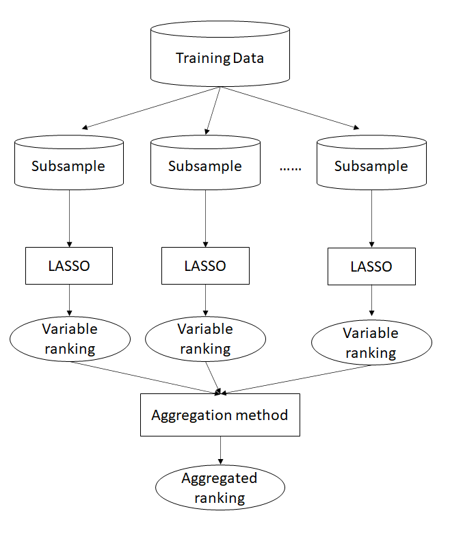
The framework of the ensemble variable selection model for shift detection consists of two phases. Firstly, we apply LASSO on a number of random subsamples of the data. For each subsample, we obtain a ranking of the variables based on the largest penalty $\lambda$ for which the variable is selected by LASSO. We aggregate the rankings from each subsample into an overall variable ranking. Secondly, we use this ranking as a basis for a variable selection method.

The foundation of ensemble learning is to combine the results of multiple models. The idea is that combining the results of several models will obtain better results by reducing the model variance and bias. Bagging and boosting are the two most commonly used ensemble models. There has been substantial recent work on the use of ensemble models for feature selection. Bolón-Canedo and Alonso-Betanzos (2018) summarize the different types of ensemble methods that are used in feature selection. We here use a homogenous scheme for the ensemble. That is, we firstly take subsamples from the training dataset, then apply LASSO to each subsample. LASSO provides a solution path by varying the penalty size. Therefore, for each subsample, a variable ranking is produced where variables are ranked in decreasing order of the largest penalty for which they are selected. Aggregating the ranking sequences from all the subsamples, we can get the overall ranking for all the variables. The process is shown in Figure 1.

Figure 1: The model structure of ensemble method for shift detection

There are several choices for how we aggregate the rankings from the different subsamples into a single overall ranking. For example, geometric mean, arithmetic mean, median, and so on. It is possible to apply these aggregation methods either to the ranking or to the values of the penalty $\lambda$. We suggest using the first quantile of the ranking to aggregate the results because the first quantile is robust to outliers. In a few subsamples, a shift may be ranked very low, possibly because the taxa that distinguish it from other shift positions are not included in the subsample. In these cases, the rank might be very large, and therefore have a large influence on the geometric or arithmetic mean. Similarly, the first quantile help improving our ability to distinguish between shifts and surrogates. It is common for only one of the surrogate variables to be ranked highly, and the shift to have a low rank. This can cause the median rank of the true shifts to be low.

After obtaining the aggregated ranking, we use model selection to choose the final combination of variables. Forward selection, backward selection, and stepwise selection are potential approaches. Forward selection starts with the null model, and sequentially adds variables in the ranked order, starting with the highest ranked, as long as the model score is better than the previous model. Backward selection starts with the full model, and sequentially removes variables in rank order, starting with the lowest ranked, as long as the model score after removing each variable is better than the previous model. Stepwise selection consists of one forward selection pass followed by one backward selection pass, starting with the model selected by forward selection. Firstly include the variables that improve the model score then remove the variables whose removal further improves the model score. From the simulation results, stepwise selection performs best.

Our procedure to estimate $\alpha$ and $\sigma^{2}$ is similar to $\ell$1ou.

1. Fit a null BM phylogenetic regression model on the dataset. Get the initial estimate of $\sigma^{2}$.

2. Use $\alpha=0$ and the $\sigma^{2}$ value from the first step to calculate the covariance matrix and apply the ensemble method selection procedure.

3. Fit the phylogenetic regression model with the selected variables in Step 2 and get new estimates of $\alpha$ and $\sigma^{2}$.

4. Repeat Step 2 and Step 3 once more.

5. Select the model with the best model criterion score

2.6 Model selection criteria

For all the models, a criterion is used to conduct model selection for the number of shifts. AIC and BIC are most the commonly used criteria in model selection problems. Ho and Ané (2014) showed that using AIC as the criterion may lead to model overfitting. Khabbazian et al. (2016) present a new criterion pBIC including a phylogenetic correction. The traditional BIC is given by:

$$\operatorname{BIC}(M_{k})=-2\operatorname{loglik}(M_{k})+(2k+3)\log(n)$$

where $n$ is the number of taxa, $k$ is the number of shifts selected, $M_{k}$ is the estimated model. $2k+3$ is the number of parameters: each shift location and magnitude is counted as a parameter and there are 3 general parameters ($\beta_{0}$, $\alpha$, and $\sigma$). The phylogenetic BIC proposed by Khabbazian et al. (2016) is given by:

$$\operatorname{pBIC}(M_{k})=-2\operatorname{loglik}(M_{k})+2k\log(2n-3)+2\log(n)+\log\text{det}((X_{M_{k}}^{\hat{\alpha}})^{T}v\Sigma_{\alpha}^{-1}X_{M_{k}}^{\hat{\alpha}})$$

where $X_{M_{k}}^{\hat{\alpha}}$ is the matrix $X^{\alpha}$ with only the columns corresponding to the k selected shifts, and $v$ is the observed trait variance. The penalty for the shift position is $2k\log(2n-3)$. The penalty for shift magnitudes and the intercept are shown in the last term. PhylogeneticEM uses penalized least squares for model selection; details are in Section 2.4.

3 Simulation studies

We conduct simulations to compare PhylogeneticEM, $\ell$1ou (pBIC/BIC) and ensemble LASSO (pBIC/BIC). The most direct method for comparison is to compare how many true shifts the methods detect and how many wrong shifts that are selected by them. However, the OU model is not completely identifiable (Bastide et al., 2017; Ho and Ané, 2014; Khabbazian et al., 2016), and even if the selected shifts are not equivalent to the true model, a good argument can be made that selecting a close surrogate shift is preferable to failing to select the shift at all. In these cases, the true positive versus false positive curve might misrepresent the performance, since neither method has a true positive, but the method that selects the surrogate has a false positive, and so is deemed to have performed worse, even though selecting the close surrogate is arguably more correct. Therefore, we include two more measurements in comparison: predictive log-likelihood and adjusted rand index. The idea of predictive log-likelihood is to compare the prediction accuracy on test data, of the selected models from different methods. Adjusted rand index evaluates how similar the clustering of the selected model is to the clustering of the true model. We can get a more comprehensive understanding of the characteristics, strengths, limitations of the methods by combining the three different measurements.

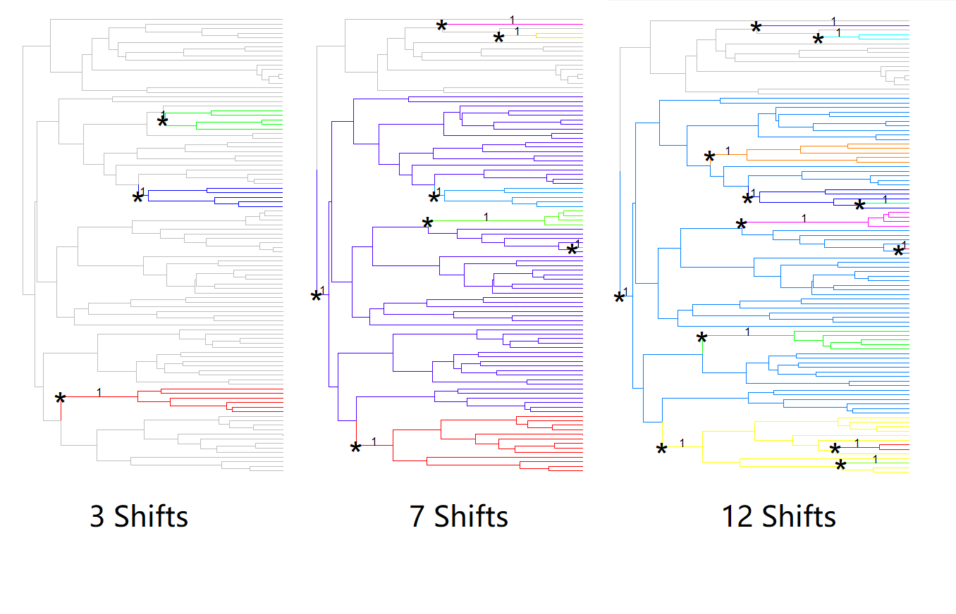
We simulate a number of scenarios with varying numbers of shifts and signal sizes. We simulate datasets under OU models along the 100-taxon Anolis lizards’ tree (Mahler, Ingram, Revell, and Losos, 2013). We compare the methods on scenarios with 3, 7, or 12 shifts. Data were simulated according to the shifts in Figure 2. For each scenario, we set $\alpha=1$ and $\sigma^{2}=2$ so that $\frac{\sigma^{2}}{2\alpha}=1$. We simulate under seven true signal sizes: $\beta=0.2,1,1.5,2,2.5,3$ and $5$. In each simulation, all shifts have the same value of $\beta$.

3.1 True positive versus false positive

Figure 2: Tree used in simulations to compare the precision and recall of different methods. The shifts positions are indicated by asterisks. Different colours indicate different optimal values for the trait.

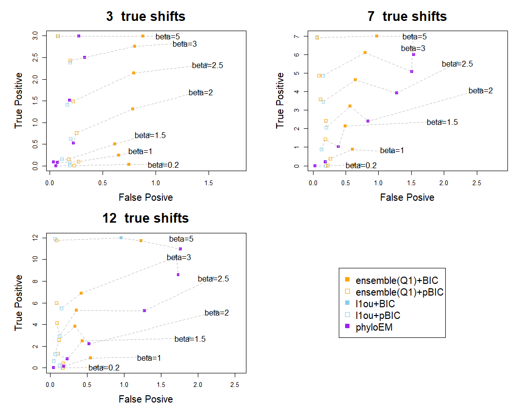
We first compare the methods by true positive versus false positive curves. True positive is the number of true shifts detected by the model. False positive is the number of shifts that are not simulated but which are wrongly detected by the model. If two models have similar false positive values, the one with a higher true positive value is considered to have a better performance. If one model has a higher true positive and higher false positive than another, there is no obvious conclusion about which model is better. It becomes a trade-off problem between precision and recall.

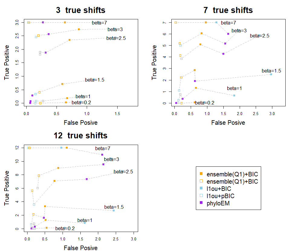
Figure 3 shows the average true positive versus false positive curve from 200 simulations in each scenario. Each point in Figure 3 represents the mean of true positive and mean of false positive values. From the simulation results, $\ell$1ou+pBIC is usually the most conservative method, with both lowest true positive and false positive. For example, in the simulation of 7 shifts and $\beta=2$, $\ell$1ou+pBIC on average detects under 2 shifts. $\ell$1ou+BIC is usually the least conservative method. Ensemble LASSO provides more balanced choices between those two methods. In most simulations, ensemble LASSO with BIC and pBIC have both higher true positive and false positive compared to $\ell$1ou+pBIC and have both lower true positive and false positive compared to $\ell$1ou+BIC. Furthermore, in some situations, ensemble LASSO methods have a better performance compared to $\ell$1ou. For example, in the simulation of 7 shifts and $\beta=2$, ensemble LASSO+pBIC has higher true positive and lower false positive compared to $\ell$1ou+pBIC and ensemble LASSO+BIC has higher true positive and lower false positive compared to $\ell$1ou+BIC. PhylogeneticEM is even more conservative than $\ell$1ou+pBIC when the signal sizes are small. It performs well where there are only 3 true shifts. However when the number of shifts and the coefficient sizes are large enough, PhylogeneticEM performs poorly compared to other methods, including more false positive and fewer true positive variables.

Figure 3: True positive numbers versus False positive numbers with 3,7,12 shifts.

3.2 Predictive log-likelihood

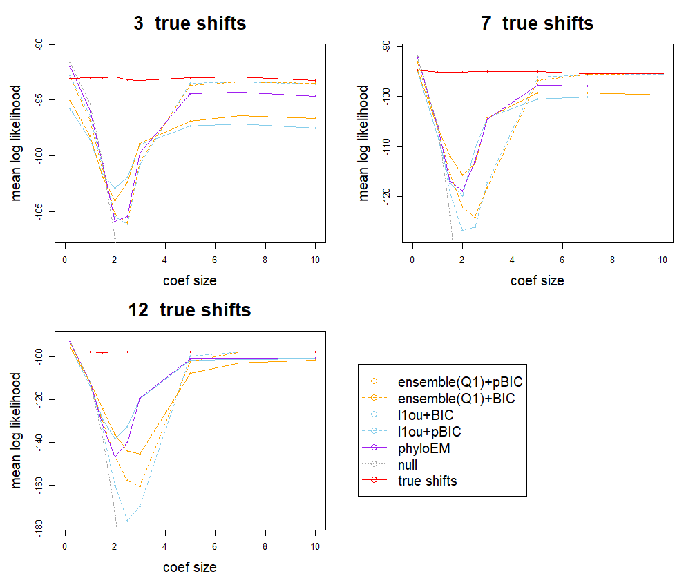
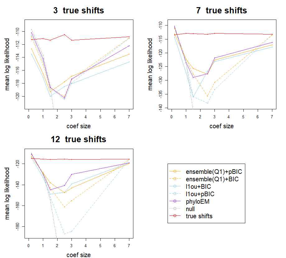
For each simulation, we generate $1000$ test datasets and $200$ training datasets. We calculate the mean of log likelihood values over $1000$ test datasets using the estimated shifts from training sets. When the results of a method give higher predictive log-likelihood value, it indicates that the method performs better at predicting the trait values. Figure 4 shows the mean of average log likelihood values over $1000$ test datasets with different numbers of true shifts and coefficient sizes.

From the simulation results, when the size of coefficients are very small or very large, methods with pBIC have a higher prediction log likelihood value. When coefficient sizes are very small, methods with pBIC are very strict and tend to select nearly no shifts. In these scenarios, the signal sizes are so small that the null model has a higher prediction likelihood compared to the true model. When coefficient sizes are very large, all the methods can detect almost all the true shifts, while the methods with BIC might include more false positive shifts. Conversely, when the coefficient sizes are in the middle of the range, methods with BIC have a better performance in terms of prediction accuracy. PhylogeneticEM is quite conservative, with high predictive log-likelihood when the signal sizes are small. And in most cases, the performance of PhylogeneticEM is between that of the pBIC and BIC methods. The difference between the ensemble method and $\ell$1ou is smaller than the difference between BIC and pBIC, and which method performs better vary between scenarios.

Figure 4: The mean log likelihood on 1000 test datasets

3.3 Adjusted rand index

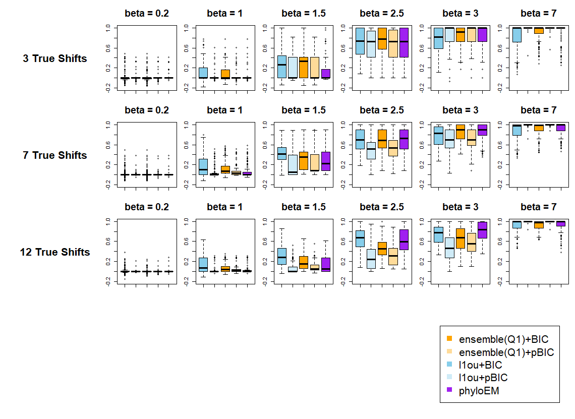
An alternative approach to assess the accuracy of the chosen shifts is to compare the induced grouping of species based on the shifts. We used adjusted rand index (ARI, Hubert and Arabie, 1985) between the clustering of tips of the true model and the clustering of the estimated shifts to evaluate the model performances. The ARI is proportional to the number of pairs in agreement between two clusterings. The ARI is scaled and centred so that identical clusterings give an ARI of 1 and the expected ARI of two random clusterings is 0.

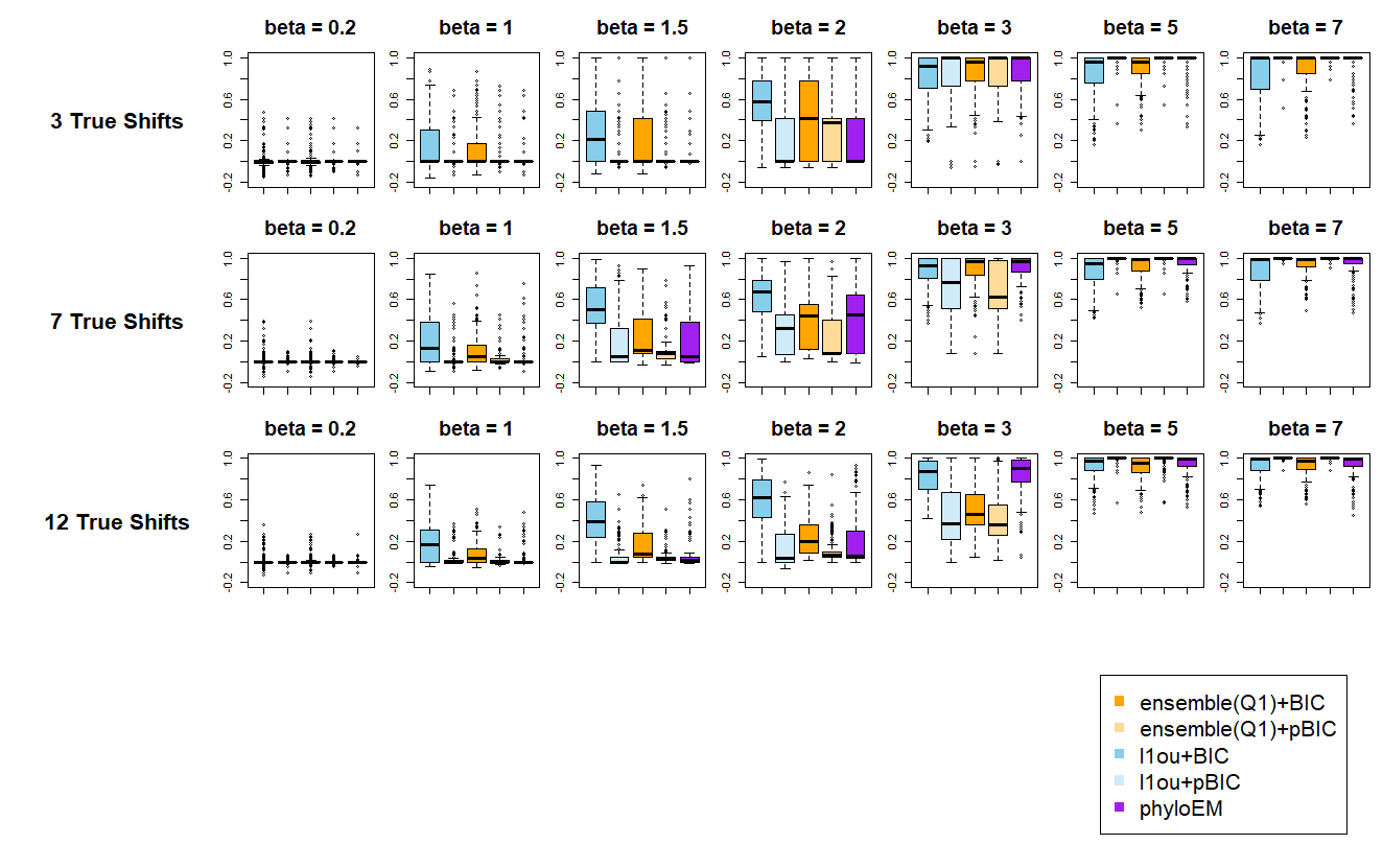
Figure 5 shows the ARI comparison of the different methods with 3, 7, and 12 shifts. ARI shows a similar result to the prediction log likelihood. When the signal sizes are small, the methods with BIC have a better performance. When the signal sizes are large enough, the methods with pBIC have a higher ARI score. PhylogeneticEM has low ARI score when the signal sizes are small and good performances when the signal sizes are in the middle. Based on true positive versus false positive numbers, PhylogeneticEM has poor performance with 7 and 12 shifts, but its predictive log-likelihood and ARI are comparable to other methods. This means that the shifts estimated by PhylogeneticEM might not be the exact true shifts, but they give similar trait predictions and trait clustering results.

Figure 5: ARI with 3, 7, 12 true shifts

4 Effect of shift position and tree on model performance

The previous simulations are all based on the same phylogenetic tree and three different shift configurations depending on the number of shifts. In this section, we perform simulations under a wider range of shift positions and phylogenetic trees, to assess the effect of these factors on the performance of the various methods.

4.1 Shifts in different positions on the tree

In this section, we study the influence of shift position. Intuitively, different shift positions influence different numbers of taxa and have different evolution time for the taxa so the results might be different. Indeed the pBIC criterion is designed specifically to account for the effect of shift position. We perform simulations with only $1$ shift in different positions on the tree (Figure 6). We perform simulations with $\beta=1,2,3,10$, $\alpha=1$ and $\sigma^{2}=2$.

Figure 6: Shifts in different positions of tree

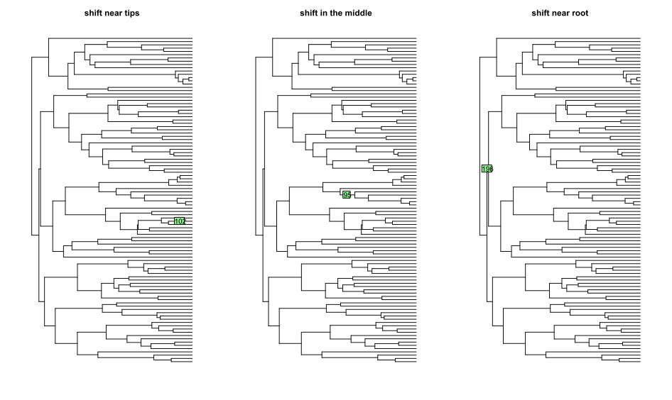
Figure 7 shows the true positive versus false positive curves of different shift positions. When the coefficient size is very large, all the methods can detect the true positive shift correctly, regardless of its position. When the coefficient size is not large enough, the shift near the root is the easiest one to detect. All the methods have higher true positive values compared to shifts in other positions. The result is in line with common sense — shifts near the root influence a large group of taxa and the evolution time after the shift is longer, so the shift might have a larger influence on the trait values, making it easier to detect. However, shifts near leaves are easier to detect compared to shifts in the middle based on the simulations for $\beta=2$ and $\beta=3$. And for $\beta=2$ and $\beta=3$, ensemble LASSO+BIC performs better than $\ell$1ou+BIC at detecting the shift near the root or the shift near the leaves. PhylogeneticEM has a good performance for detecting the shift near the root but has worse performance for detecting the shift near the leaves and the shift in the middle.

Figure 7: True positive versus false positive with different shift positions

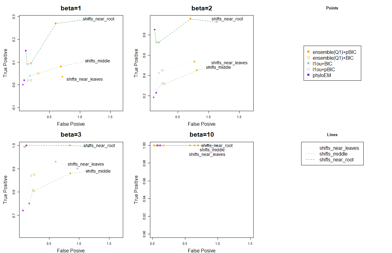
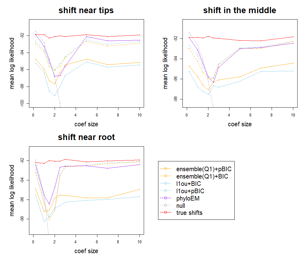
Figure 8 shows the predictive log-likelihood of the methods for different shift positions. We only include 1 shift in these simulations, and a conservative method usually has a higher prediction likelihood when the number of shifts is small. Thus, for the shift near the leaves and the shift in the middle, for predictive log-likelihood, $\ell$1ou+pBIC $>$ ensemble LASSO+pBIC $>$ ensemble LASSO+BIC $>$ $\ell$1ou+BIC. However, for the simulations with the shift near the root, ensemble LASSO shows its strength when the coefficient size is in the middle of the range. Figure 9 shows the ARI of methods with different shift positions. Comparing the model performances on the scenarios with different positions of shift by ARI, all the methods perform better with the shift near the root, then shift near the middle, and perform worst with the shift near the leaves. This may be because of the way ARI is defined. For a shift on a leaf branch, the ARI of a close surrogate shift is still relatively low, whereas, for shifts near the root or the middle of the tree, close surrogate shifts have a significantly higher ARI.

Figure 8: Log test likelihood with different shift positions

Figure 9: ARI with different shift positions

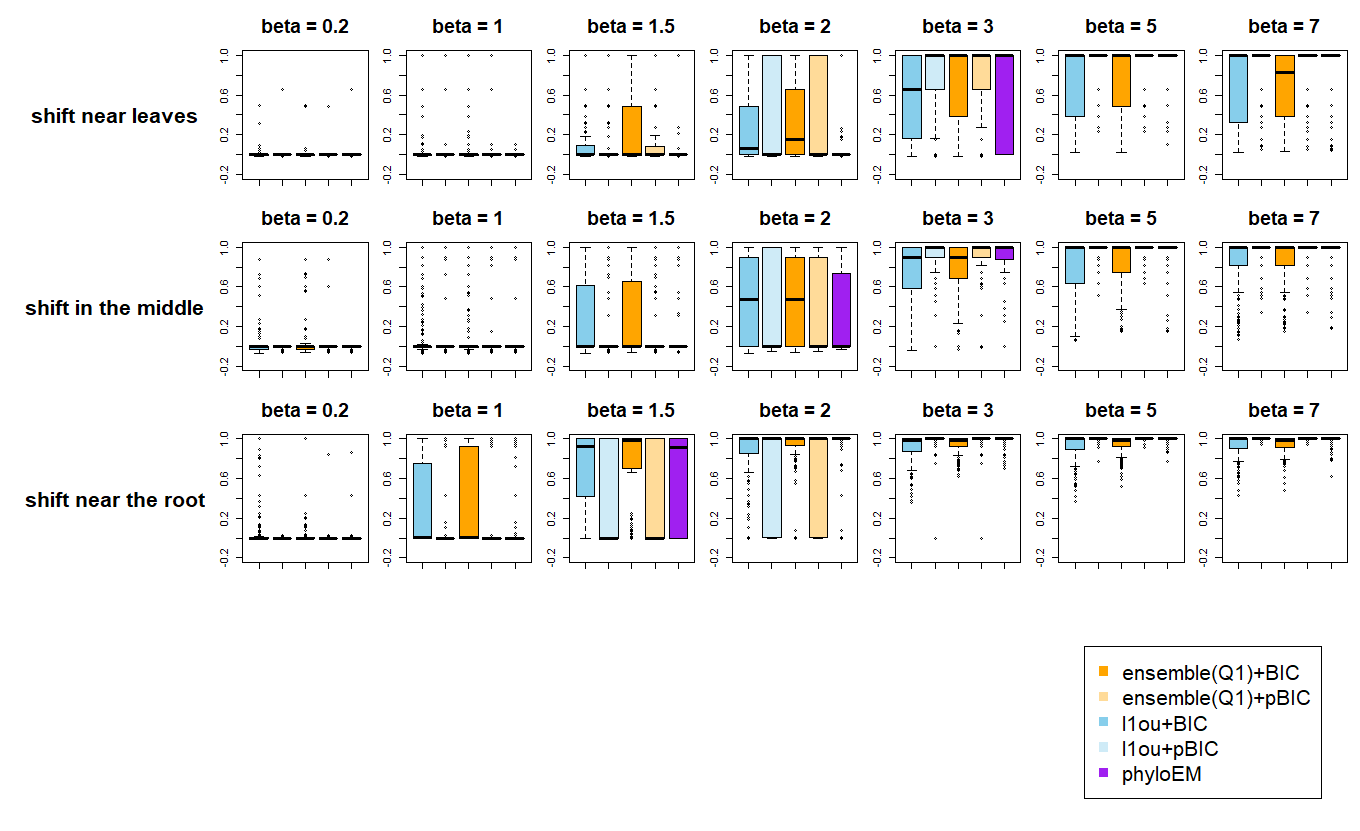
4.2 Different types of tree

In this section, we compare the model performances on shift detection tasks on different types of phylogenetic trees. We mainly consider 4 types of tree: balanced tree, caterpillar tree, pure birth tree and coalescent tree. We generate these 4 types of trees with 128 taxa and 254 edges. Figure 10 shows the generated tree and simulated shifts for each type of tree. In this simulation, there are 3 shifts on each tree.

Figure 10: 4 different types of tree

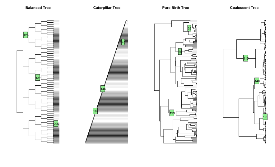
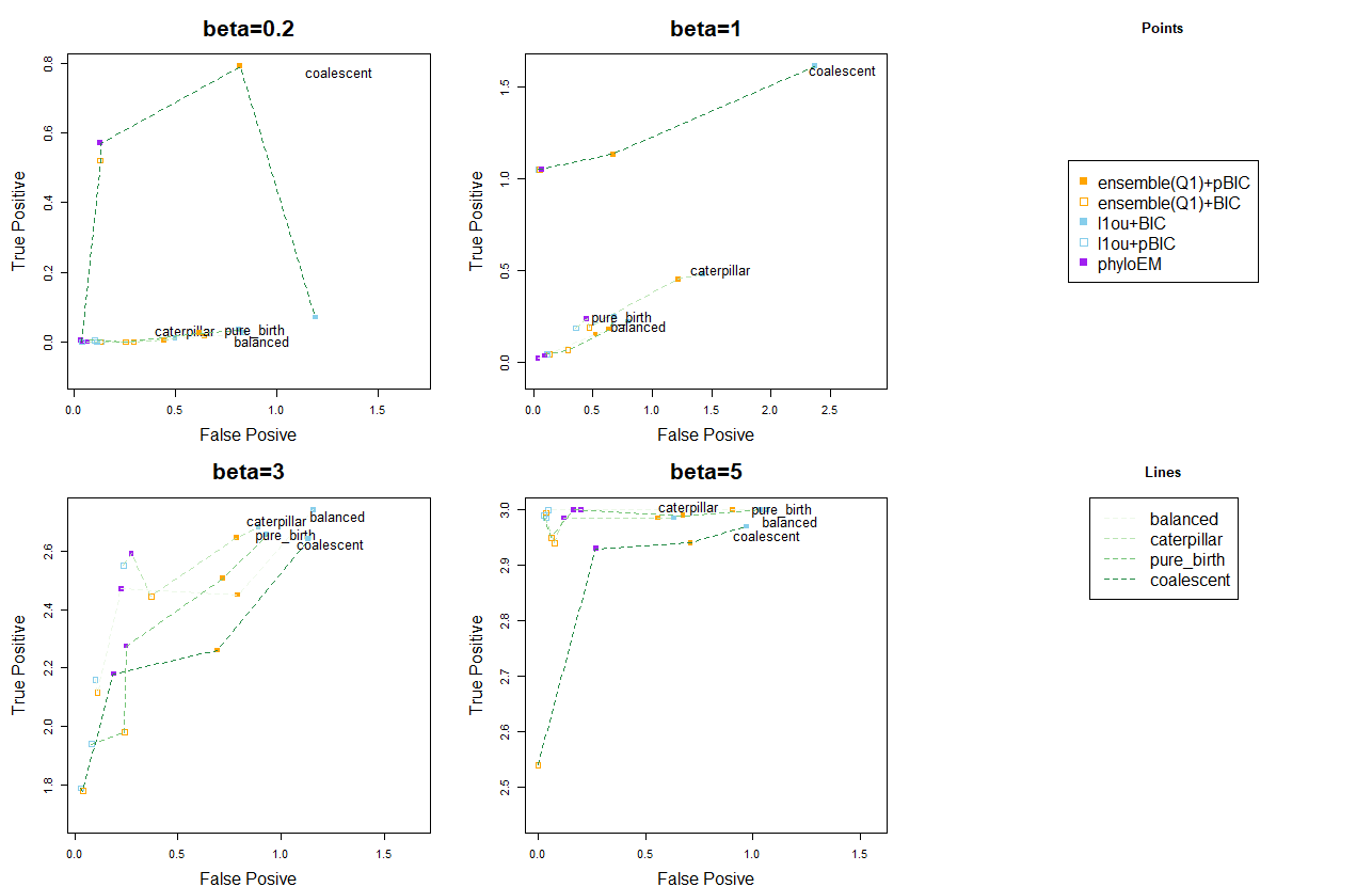
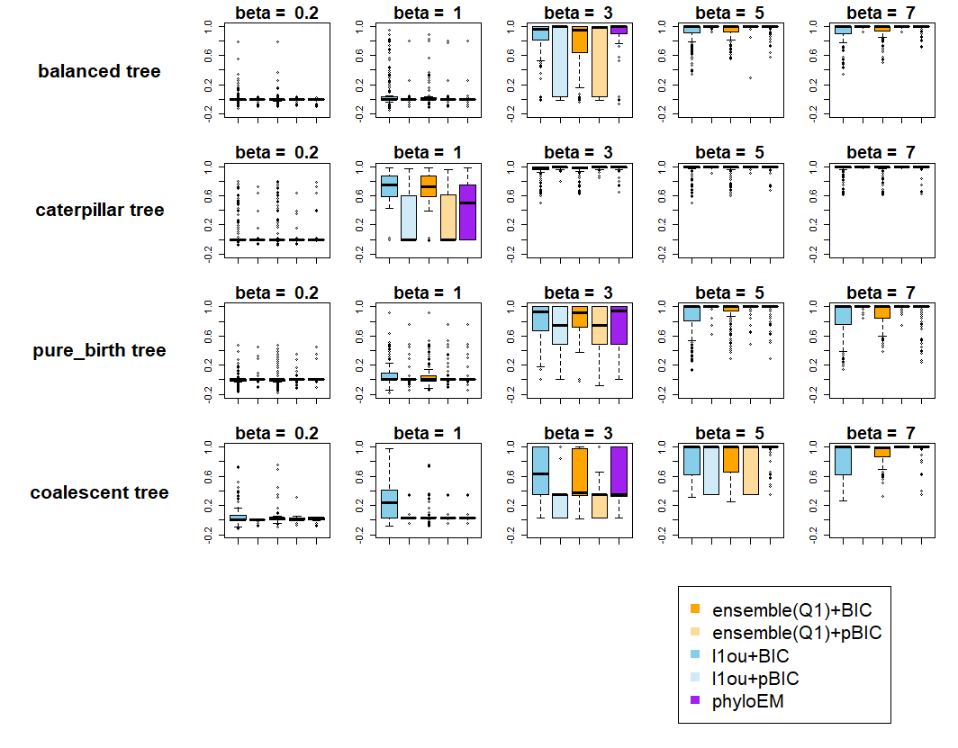
Figure 11 shows the true positive versus false positive curves for different types of trees. Interestingly, the shifts in the coalescent tree are the easiest to detect when the coefficient size is small and the most difficult to detect when the coefficient size is large. Especially for ensemble LASSO, when $\beta=0.2$, ensemble LASSO+BIC has a much higher true positive compared to other methods and a lower false positive compared to $\ell$1ou+BIC. For other types of tree, generally speaking when the coefficient size is in the middle of the range, the shifts on the caterpillar tree are the easiest to detect, and then the balanced tree, then the pure birth tree and finally the coalescent tree. Figure 12 shows the predictive log-likelihood. It is obvious that ensemble methods perform very well on the coalescent tree with small signal size and poorly with large signal size. Figure 13 shows the ARI with different types of trees. From the ARI results, the order of difficulties of shift detection on different types of trees is coalescent tree $>$ pure birth tree $>$ balanced tree $>$ caterpillar tree.

Figure 11: True positive versus false positive with different types of trees

Figure 12: Average test log likelihood with different types of trees

Figure 13: ARI with different types of trees

5 Robustness to violations of model assumptions

The simulations above assume that the model assumptions in Section 2 are met. However, in reality, the real data often violate the model assumptions. For example, the trait values might contain measurement errors. Measurement errors enlarge the variance of the data and make accurate detection more difficult. Another example is that the phylogenetic tree is constructed based on sequence data, thus can also have errors. These kinds of problems are hard to avoid in real data analysis. It is, therefore, important to consider how the methods perform when the model assumptions are not satisfied. In this section, we discuss several violations of model assumptions. We also study the effects of misestimation of parameters on model selection performance. Because the $\ell$1ou and ensemble methods use a very crude approach to estimate $\alpha$, it is important to examine the question of how misestimation of $\alpha$ impacts results. PhylogeneticEM does not suffer from this problem because it does not have a preconditioning step.

5.1 Measurement errors

It is common for the measurement of traits to be subject to errors. These errors may impact the shift detection methods, which assume that the trait values are measured perfectly. In this section, we simulate additive Gaussian measurement error $N(0,\sigma_{e}^{2})$ for the trait value of each species. When $\sigma_{e}^{2}$ is larger, the size of the measurement error is larger.

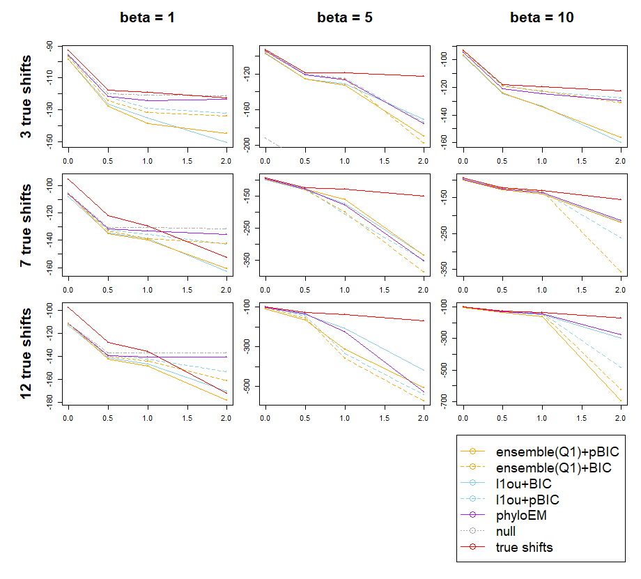
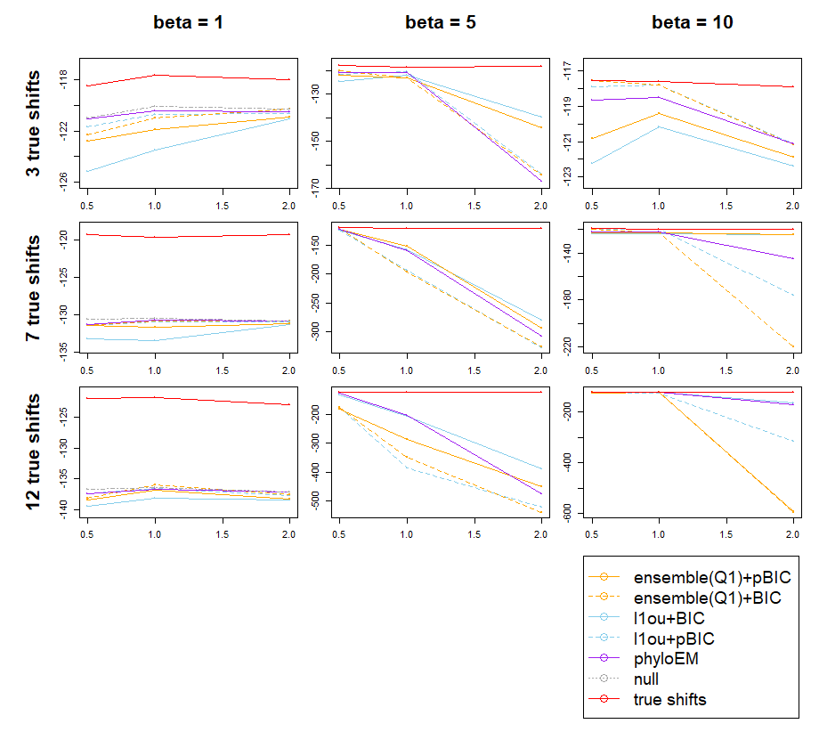
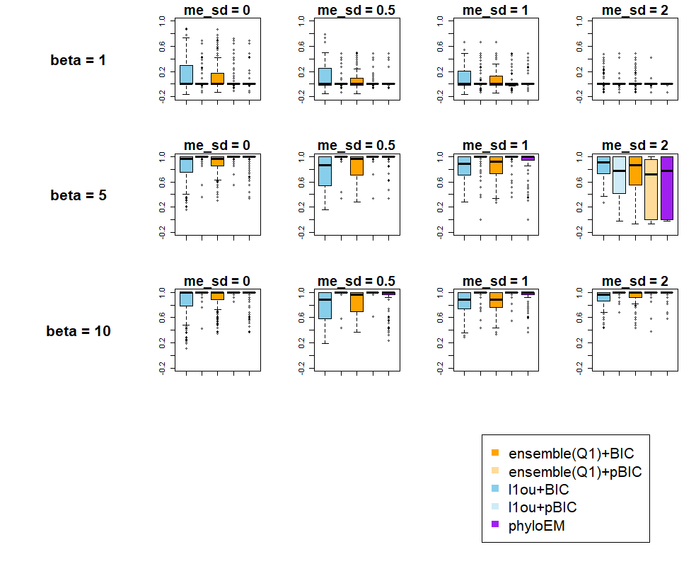
Figure 14 shows the true positive versus false positive with changing measurement errors. Figure 15 shows the predictive log-likelihood value with changing measurement errors in training data. Because of the measurement errors in the training data, the true shift model has a lower log-likelihood than the null model. If we use the training data with measurement error to estimate the parameters of selected shifts, the parameters will be far from the real values and thus introduce errors while calculating the predictive log-likelihood. Since our purpose is to identify the true shifts, predictive log-likelihood using training data with measurement error to estimate the parameters is not an ideal way to assess the selected shifts. Therefore, we also compare the prediction log-likelihood of the shift detection methods using the training data with measurement error to select shifts, but with parameters estimated from training data without measurement error. Figure 16 shows the results of log likelihood with parameters estimated from training data without measurement error. Figure 17 shows the ARI with measurement error. The plots show that the measurement error will influence the accuracy of shift detection. The loss of accuracy increases with the number of shifts. The performance of all the methods worsens with measurement error. When the signal is not so strong ($\beta=1$), even a relatively small measurement error severely impacts performance. Interestingly, in terms of ARI, when $\beta=10$, the performance of the methods using BIC improves with increased measurement error. Looking at the true and false positive rates, we see that the methods consistently select the true variables, but with increased measurement error, the false positive rate is reduced. However, the predictive log-likelihood does decrease. This may be because even though failing to select a true variable is very rare in this case, it has a huge impact on the log-likelihood, because of the strong signal strength. Thus the effect on predictive log-likelihood may be driven by the small number of cases where a true variable is missed.

Figure 14: True positive versus false positive with changing measurment error.

Figure 15: Average test log likelihood with parameters estimated from training data with measurement error

Figure 16: Average test log likelihood with parameters estimated from training data without measurement error

Figure 17: Distribution of ARI between selected shift configuration and true shift configuration with changing measurment error.

5.2 Brownian-Motion model

Another assumption that may be violated is that the evolution on each branch follows an OU process. In this section, we use BM to simulate the trait values. This is a very simple simulation of this violation since BM is a special case of the OU process with $\alpha=0$. Other models should be considered in future studies.

Based on the results of Figures 18, 19, and 20, under the BM model, the results are similar compared to the results under the OU model. There is no significant failure of any method when applied to data generated from the BM model. The strength of ensemble LASSO methods when there are 7 or 12 shifts becomes more obvious. Ensemble LASSO+BIC has a lower false positive rate compared to $\ell$1ou+BIC and similar or even higher true positive rate. Ensemble LASSO+pBIC has a higher true positive rate compared to $\ell$1ou+pBIC and similar or even lower false positive rate.

Figure 18: True positive versus false positive with BM model.

Figure 19: Average test log likelihood with BM model.

Figure 20: ARI with BM model. 3 true shifts simulations are shown in this figure.

5.3 Incorrect tree

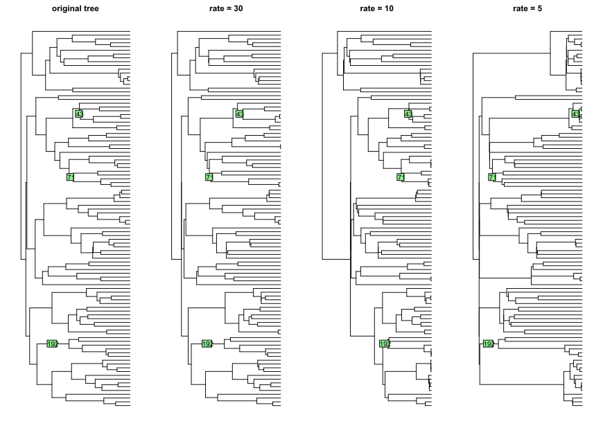
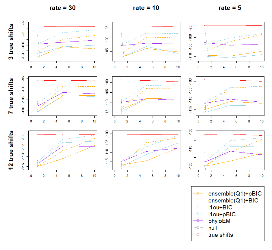
Another possible violation is that we use a wrong tree to do the shift detection. There are two possible errors in the analyzed tree: wrong topology or wrong branch lengths. In the case of an incorrect topology, it is not always clear that there is a meaningful way to define “true shifts” in a false tree. Therefore, we will focus on the case with incorrectly specified branch lengths. We simulate data from a tree with different branches and apply the methods to the originally provided tree. We use a gamma distribution ($Gamma(\beta*\mathrm{original\ branch\ length},\beta)$) to randomly generate each internal branch length. Thus, the mean of each branch length is the original branch length, and the variance is larger for smaller $\beta$. In order to generate ultrametric trees and keep the total tree depth the same as the original tree, the external branches are generated by the original tree depth minus the tree depth of the starting node of each external branch. The internal branches are generated with a depth first order. If the depth of one internal branch is larger than the given tree depth, this branch length is resampled. We generate 3 trees with $\beta=30,10,5$ as shown in Figure 21.

Figure 21: Regenerated tree with different beta

Firstly, we find that this violation of assumptions can cause convergence problems while iterating the methods to estimate $\alpha$ in $\ell$1ou or the ensemble method. This is a problem we observe for real data in Section 6. Figure 22 shows the number of cases where the estimated alpha does not converge in 10 iterations out of 200 simulations. The convergence problems seem to particularly affect the ensemble method but are also present for $\ell$1ou. For the non-converging simulations, we present results for the best $\alpha$ value attempted (in terms of our model selection criterion).

Figure 22: Number of non-converging cases while analyzing on a misspecified tree

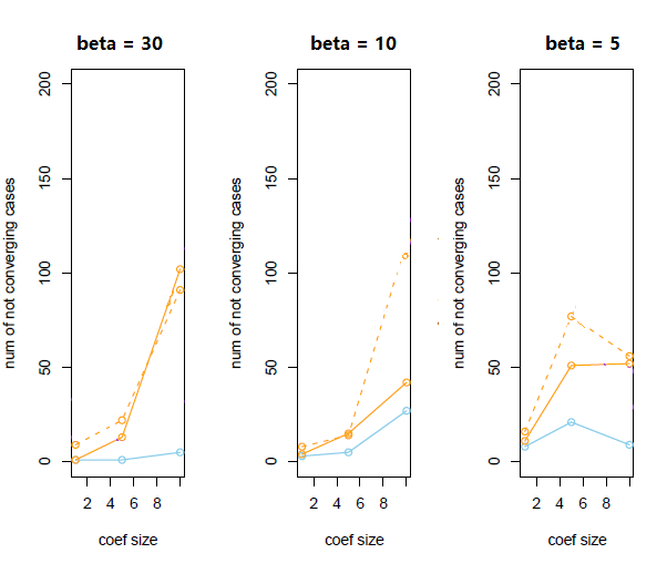
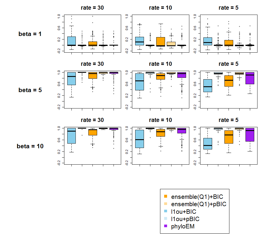
Figure 23 shows the average number of true and false positives for each misspecified tree. Figure 24 shows the prediction log-likelihood. Figure 25 shows the ARI between the estimated and true shift configurations. We see that generally speaking, the difference between the real tree and the analyzed tree will worsen the performance of the methods by either lowering the true positive rate or increasing the false positive rate. However, the methods are relatively robust to this misspecification. PhyloEM appears to be most influenced by the misspecification, becoming less conservative when the tree is misspecified. This increases both the true positive rate and the false positive rate. The predictive log-likelihood on test data is fairly robust to the tree misspecification. However, the ARI decreases, particularly for the cases with strong signals, as the tree becomes more misspecified.

In some exceptional cases, the methods perform better when the tree is misspecified. For example, for simulations with 7 or 12 true shifts, nearly all the methods got higher true positive rates when the tree was most misspecified (rate parameter = 5) than for the original tree.

Figure 23: True positive versus false positive with applying methods on misspecified trees

Figure 24: Average test log likelihood with applying methods on misspecified trees

Figure 25: ARI with methods applied on misspecified trees

5.4 Misestimation of $\alpha$

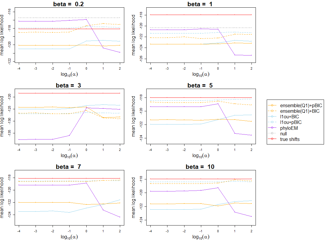
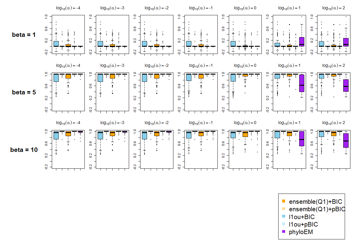
Recall from Section 2 that both $\ell$1ou and ensemble use a very rough method to estimate $\alpha$. This could lead to the estimated $\alpha$ values being very bad. In this section, we investigate the extent to which misestimation of $\alpha$ can impact the variable selection results. In this simulation, we use $\alpha=1$ to generate data and use different $\hat{\alpha}$ $(10^{-4},10^{-3},...,10^{2})$ in the methods and compare the model performances.

Figure 24 and Figure 25 show the prediction log likelihood and ARI with different estimated $\hat{\alpha}$. From the plots, the performance of PhylogeneticEM is influenced most by changes in the estimation of $\alpha$. Especially when the estimated $\alpha$ is too large, the method performs poorly. Ensemble methods and $\ell$1ou are more robust to misestimation of $\alpha$. Since PhlyoEM uses maximum likelihood to estimate $\alpha$, which is expected to produce more accurate estimates, robustness to misestimation is less important than for $\ell$1ou and the ensemble method, which use a very rough method to estimate $\alpha$.

Figure 26: Average test log likelihood with changing estimated alpha

Figure 27: ARI with changing estimated alpha

6 Case study: Anolis Lizard data

The tree and trait data of Anolis lizards are provided by Mahler et al. (2013). They applied PCA to 11 traits including body size, limb, tail length, and so on. They found that the first four principal components explained 93% of the variation. The data are available in the R package $\ell$1ou. We compare the results of the different variable selection methods for the Anolis Lizard data.

6.1 Results

Figure 28: Shifts detected by different models for lizard data

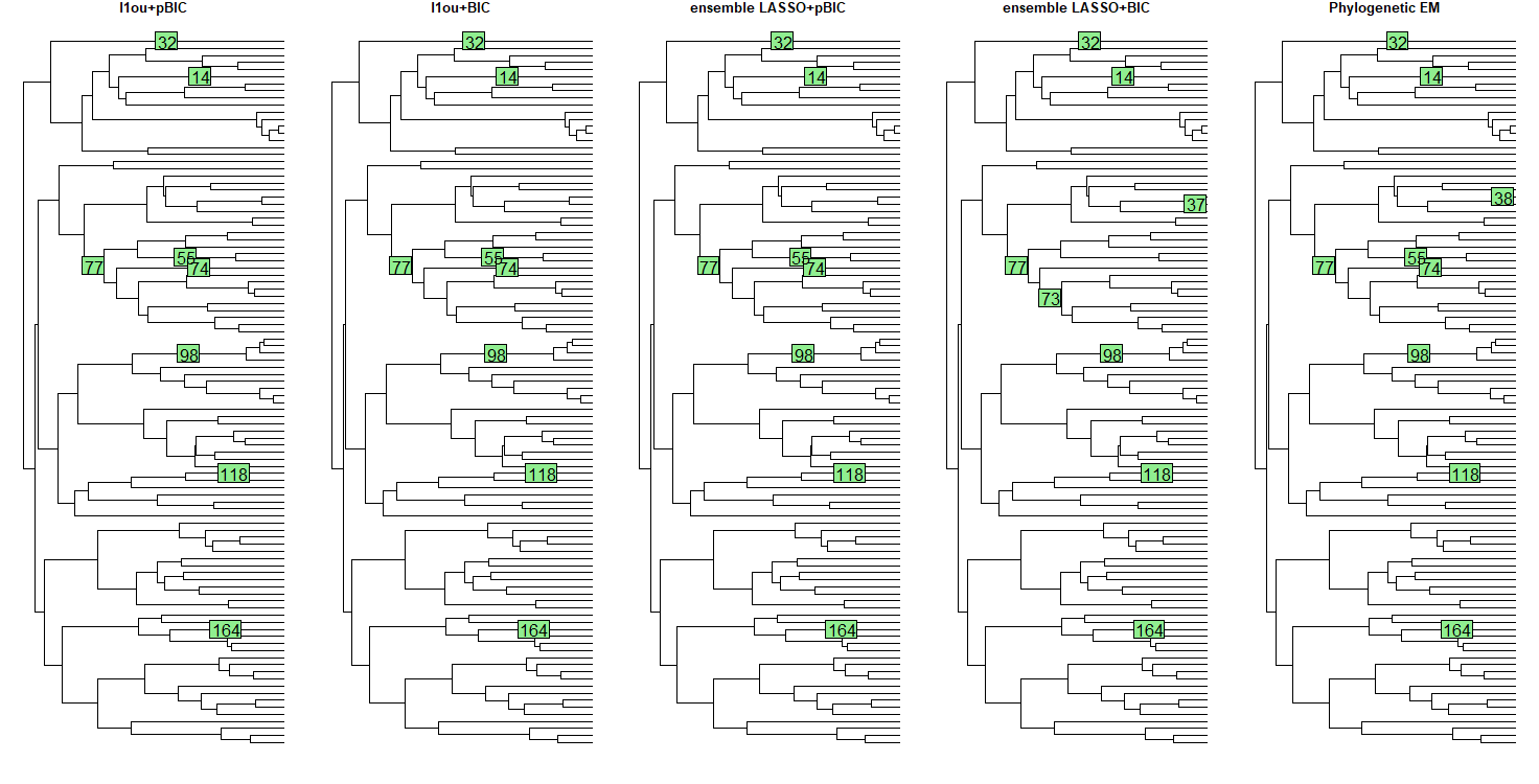
Figure 27 shows the shifts detected by applying $\ell$1ou+pBIC, $\ell$1ou+BIC, ensemble LASSO+pBIC, ensemble LASSO+BIC, and PhylogeneticEM on the first principal component of the lizard traits. All the methods have similar results. $\ell$1ou+pBIC, $\ell$1ou+BIC and ensemble LASSO+pBIC detected the same shifts. Ensemble LASSO+BIC has slightly different results, only differing for a small number of species. Both ensemble LASSO+BIC and PhylogeneticEM detect one more shift near the leaf node that the other three methods do not select. The estimated shift sizes range from $-5.50$ to $-1.91$. By applying several methods to the same dataset, we might say that the shifts which are selected by all the five methods are highly likely to be true. While the shifts which are selected by only one or two methods might need further investigation and more biological evidence.

There are also convergence problems for the estimation of $\alpha$ for this real dataset. From Section 5.3, this might indicate that the tree is misspecified, or some other violation of the model assumptions.

6.2 Recommendations

We suggest applying multiple methods to each data set and comparing the results. Based on the simulation results, different methods have different strengths and we cannot say that any method outperforms the others in every situation. For example, the methods with pBIC are the most conservative: they perform best with large signal sizes. They can detect the true shifts without introducing false positive shifts. However, they cannot give reasonable results when the signal sizes are small. The ensemble method with BIC can better capture the shifts near the leaves. PhylogeneticEM is even more conservative with small signal sizes and falls between methods with pBIC and with BIC, with large signal sizes. It is hard to tell which method and criterion is the most suitable to use in a specific task. By comparing the results of different methods, we can get the confidence level of the selected shifts. For example for the Anolis lizard data, the shifts which are selected by all the five methods are highly likely to be true. Khabbazian et al. (2016) use bootstrap support to evaluate how likely the selected shifts are true. However, the bootstrap support can be influenced by biases in a particular method. By combing the results of several different methods, we can assess the confidence of particular shifts in a way that is unlikely to be influenced by the bias of any particular method.

7 Conclusion

In this article, we compared the performances of several shift detection methods — $\ell$1ou, PhylogeneticEM, ensemble method — for trait evolution models. To understand the strength, weaknesses, and restrictions of different methods, we compared the performances over a large range of scenarios. We used three different measurements to compare the results, true positive versus false positive curve, predictive log-likelihood and adjusted rand index.

From the simulation results, when the coefficients are very small, PhylogeneticEM, $\ell$1ou+pBIC and ensemble+pBIC are very strict and tend to select nearly no shifts. In these scenarios, ensemble+BIC and $\ell$1ou+BIC perform better at detecting the small magnitude shifts. However when the coefficients are large, nearly all the methods can detect the true shifts, but $\ell$1ou+BIC and ensemble+BIC include more false positive shifts. The performances of methods are highly dependent on the criterion. A better criterion might help the methods to give very good results with varying signal sizes. Further research about appropriate model selection criteria for shift detection might be an interesting topic for future studies.

Furthermore, we compared the model performances on different shift positions in trees and different types of trees. From the results, the shifts near the leaves are the most difficult to detect and the shifts near the root are the easiest to detect. The shifts on the coalescent tree are the easiest to detect when the coefficient is small and the most difficult to detect when the coefficient is large.

We also conducted simulations in several scenarios where the model assumptions do not hold. We studied training data with measurement error; misspecified phylogenetic trees; a non-OU model; and misestimation of the parameter $\alpha$. From the simulation results, measurement error and a misspecified phylogenetic tree cause shift detection more difficult and all the methods perform worse in these cases. $\ell$1ou and the ensemble method are robust to misestimation of $\alpha$. The simulations under a BM model in this article do not cause much difficulty. However, further research into different model misspecifications is still necessary.

In the Anolis Lizard real data case study, all five methods estimate similar shift configurations. There are only a few differences in the shifts near the leaves. The shifts which are selected by all the five methods are highly likely to be true, while the shifts which are selected by only one or two methods might need further investigation. Interestingly, we observe convergence problems for the estimation of $\alpha$ for this real data with $\ell$1ou and the ensemble method. In our simulations, estimation on training data with a misspecified tree often led to this convergence problem, which suggests that the Anolis Lizard tree may be misestimated.

8 Data accessibility

The tree and trait data of Anolis lizards are provided by Mahler et al. (2013). Our R package is available at https://github.com/WenshaZ/ELPASO.

References

- Baraud et al. (2009) Yannick Baraud, Christophe Giraud, and Sylvie Huet. Gaussian model selection with an unknown variance. The Annals of Statistics, 37(2), 2009. doi: 10.1214/07-aos573.
- Bastide et al. (2017) Paul Bastide, Mahendra Mariadassou, and Stéphane Robin. Detection of adaptive shifts on phylogenies by using shifted stochastic processes on a tree. Journal of the Royal Statistical Society: Series B (Statistical Methodology), 79(4):1067–1093, 2017. doi: 10.1111/rssb.12206.
- Bastide et al. (2018) Paul Bastide, Cécile Ané, Stéphane Robin, and Mahendra Mariadassou. Inference of adaptive shifts for multivariate correlated traits. Systematic Biology, 67(4):662–680, 2018. doi: 10.1093/sysbio/syy005.
- Bastide et al. (2021) Paul Bastide, Lam Si Tung Ho, Guy Baele, Philippe Lemey, and Marc A. Suchard. Efficient bayesian inference of general gaussian models on large phylogenetic trees. The Annals of Applied Statistics, 15(2), 2021. doi: 10.1214/20-aoas1419.
- Beaulieu et al. (2012) Jeremy M Beaulieu, Dwueng-Chwuan Jhwueng, Carl Boettiger, and Brian C O’Meara. Modeling stabilizing selection: expanding the ornstein–uhlenbeck model of adaptive evolution. Evolution: International Journal of Organic Evolution, 66(8):2369–2383, 2012.
- Bolón-Canedo and Alonso-Betanzos (2018) Verónica Bolón-Canedo and Amparo Alonso-Betanzos. Ensembles for feature selection. Intelligent Systems Reference Library Recent Advances in Ensembles for Feature Selection, page 53–81, 2018. doi: 10.1007/978-3-319-90080-3“˙4.
- Butler and King (2004) Marguerite A. Butler and Aaron A. King. Phylogenetic comparative analysis: A modeling approach for adaptive evolution. The American Naturalist, 164(6):683–695, 2004. doi: 10.1086/426002.
- Davis et al. (2007) Charles C. Davis, Maribeth Latvis, Daniel L. Nickrent, Kenneth J. Wurdack, and David A. Baum. Floral gigantism in rafflesiaceae. Science, 315(5820):1812–1812, 2007. doi: 10.1126/science.1135260.
- Dempster et al. (1977) A. P. Dempster, N. M. Laird, and D. B. Rubin. Maximum likelihood from incomplete data via theemalgorithm. Journal of the Royal Statistical Society: Series B (Methodological), 39(1):1–22, 1977. doi: 10.1111/j.2517-6161.1977.tb01600.x.
- Felsenstein (1985) Joseph Felsenstein. Phylogenies and the comparative method. The American Naturalist, 125(1):1–15, 1985. doi: 10.1086/284325.
- Gill et al. (2016) Mandev S. Gill, Lam Si Tung Ho, Guy Baele, Philippe Lemey, and Marc A. Suchard. A relaxed directional random walk model for phylogenetic trait evolution. Systematic Biology, 2016. doi: 10.1093/sysbio/syw093.
- Hansen (1997) Thomas F. Hansen. Stabilizing selection and the comparative analysis of adaptation. Evolution, 51(5):1341, 1997. doi: 10.2307/2411186.
- Hassler et al. (2020) Gabriel Hassler, Max R. Tolkoff, William L. Allen, Lam Si Tung Ho, Philippe Lemey, and Marc A. Suchard. Inferring phenotypic trait evolution on large trees with many incomplete measurements. Journal of the American Statistical Association, page 1–15, 2020. doi: 10.1080/01621459.2020.1799812.
- Ho and Ané (2013) Lam Si Tung Ho and Cécile Ané. Asymptotic theory with hierarchical autocorrelation: Ornstein–uhlenbeck tree models. The Annals of Statistics, 41(2):957–981, 2013.
- Ho and Ané (2014) Lam Si Tung Ho and Cécile Ané. Intrinsic inference difficulties for trait evolution with ornstein-uhlenbeck models. Methods in Ecology and Evolution, 5(11):1133–1146, 2014. doi: 10.1111/2041-210x.12285.
- Hubert and Arabie (1985) Lawrence Hubert and Phipps Arabie. Comparing partitions. Journal of Classification, 2(1):193–218, 1985. doi: 10.1007/bf01908075.
- Ingram and Mahler (2013) Travis Ingram and D.Luke Mahler. Surface: Detecting convergent evolution from comparative data by fitting ornstein-uhlenbeck models with stepwise akaike information criterion. Methods in Ecology and Evolution, 4(5):416–425, 2013. doi: 10.1111/2041-210x.12034.
- Jaffe et al. (2011) Alexander L. Jaffe, Graham J. Slater, and Michael E. Alfaro. The evolution of island gigantism and body size variation in tortoises and turtles. Biology Letters, 7(4):558–561, 2011. doi: 10.1098/rsbl.2010.1084.
- Khabbazian et al. (2016) Mohammad Khabbazian, Ricardo Kriebel, Karl Rohe, and Cécile Ané. Fast and accurate detection of evolutionary shifts in ornstein–uhlenbeck models. Methods in Ecology and Evolution, 7(7):811–824, 2016. doi: 10.1111/2041-210x.12534.
- Lee and Leu (2011) Chien-Pang Lee and Yungho Leu. A novel hybrid feature selection method for microarray data analysis. Applied Soft Computing, 11(1):208–213, 2011. doi: 10.1016/j.asoc.2009.11.010.
- Losos (2011) Jonathan B. Losos. Lizards in an evolutionary tree: Ecology and adaptive radiation of anoles. University of California Press, 2011.
- Mahler et al. (2013) D. Luke Mahler, Travis Ingram, Liam J. Revell, and Jonathan B. Losos. Exceptional convergence on the macroevolutionary landscape in island lizard radiations. Science, 341(6143):292–295, 2013. doi: 10.1126/science.1232392.
- Mera-Gaona et al. (2021) Maritza Mera-Gaona, Diego M. López, and Rubiel Vargas-Canas. An ensemble feature selection approach to identify relevant features from eeg signals. Applied Sciences, 11(15):6983, 2021. doi: 10.3390/app11156983.
- Pes (2019) Barbara Pes. Ensemble feature selection for high-dimensional data: A stability analysis across multiple domains. Neural Computing and Applications, 32(10):5951–5973, 2019. doi: 10.1007/s00521-019-04082-3.
- Piao et al. (2012) Y. Piao, M. Piao, K. Park, and K. H. Ryu. An ensemble correlation-based gene selection algorithm for cancer classification with gene expression data. Bioinformatics, 28(24):3306–3315, 2012. doi: 10.1093/bioinformatics/bts602.
- Uyeda and Harmon (2014) Josef C. Uyeda and Luke J. Harmon. A novel bayesian method for inferring and interpreting the dynamics of adaptive landscapes from phylogenetic comparative data. Systematic Biology, 63(6):902–918, 2014. doi: 10.1093/sysbio/syu057.
- Zhang and Siegmund (2006) Nancy R. Zhang and David O. Siegmund. A modified bayes information criterion with applications to the analysis of comparative genomic hybridization data. Biometrics, 63(1):22–32, 2006. doi: 10.1111/j.1541-0420.2006.00662.x.