Variable importance measures for heterogeneous causal effects

Abstract

The recognition that personalised treatment decisions lead to better clinical outcomes has sparked recent research activity in the following two domains. Policy learning focuses on finding optimal treatment rules (OTRs), which express whether an individual would be better off with or without treatment, given their measured characteristics. OTRs optimize a pre-set population criterion, but do not provide insight into the extent to which treatment benefits or harms individual subjects. Estimates of conditional average treatment effects (CATEs) do offer such insights, but valid inference is currently difficult to obtain when data-adaptive methods are used. Moreover, clinicians are (rightly) hesitant to blindly adopt OTR or CATE estimates, not least since both may represent complicated functions of patient characteristics that provide little insight into the key drivers of heterogeneity. To address these limitations, we introduce novel nonparametric treatment effect variable importance measures (TE-VIMs). TE-VIMs extend recent regression-VIMs, viewed as nonparametric analogues to ANOVA statistics. By not being tied to a particular model, they are amenable to data-adaptive (machine learning) estimation of the CATE, itself an active area of research. Estimators for the proposed statistics are derived from their efficient influence curves and these are illustrated through a simulation study and an applied example.

Keywords: Causal inference; Conditional effects; Effect modification; Data-adaptive estimation

1 Introduction

In the medical and social sciences there has been a longstanding interest in quantifying heterogeneity in the effects of treatments or interventions between groups of individuals. Understanding such heterogeneity is essential, for instance, in informing scientific research and optimising treatment decisions. Attention focused initially on subgroup analyses, which identify population subgroups (defined in terms of pre-treatment covariates) that benefit most/least from treatment, to be evaluated further in potential future studies; see e.g. Rothwell, (2005) for a review, and Slamon et al., (2001) for the first clinical trial in oncology that was restricted to targeted trial populations. Typical challenges of subgroup analyses are how to select stratification variables in a systematic way, and how to handle the resulting multiplicity problem. Endeavours to address these were soon followed by methodological developments on personalised medicine in the causal inference literature, pioneered by Murphy, (2003).

For many years, the primary focus in the causal inference literature was on policy learning; that is, determining the treatment policy (which assigns the same treatment to individuals with the same measured covariate values) that minimizes some measure of population risk (van der Laan and Luedtke,, 2014; Kallus,, 2021; Athey and Wager,, 2021). More recently, attention has partially shifted towards (machine-learning based) estimation of conditional average treatment effects (CATEs) (Abrevaya et al.,, 2015; Athey and Imbens,, 2016; Nie and Wager,, 2021; Wager and Athey,, 2018; Künzel et al.,, 2019; Kennedy,, 2020). Letting $Y^{a}$ denoting the outcome that would be observed if treatment $A$ were set to $a\in\{0,1\}$, and $\bm{X}\in\mathbb{R}^{p}$ a vector of pre-treatment covariates, the CATE can be defined as $\tau(\bm{x})\equiv E(Y^{1}-Y^{0}|\bm{X}=\bm{x})$ (Rubin,, 1974). Estimates of the CATE can also been used for policy learning, for instance, the so-called optimal dynamic treatment rule (OTR) for an individual with covariate value $\bm{x}$, assigns treatment based on the sign of $\tau(\bm{x})$ (VanderWeele et al.,, 2019). The CATE, however, additionally provides insight into the magnitude of the treatment effect for these individuals.

These foregoing developments are extremely useful and important, but leave unanswered a key question that researchers commonly have when presented with an estimated CATE or OTR: namely, what are the key drivers of treatment effect heterogeneity? In the context of policy learning, attempts to find the optimal policy within a restricted class of ‘simple’ policies go some way towards answering this question, albeit at the risk of targeting a suboptimal policy (Zhang et al.,, 2015). In this paper, we instead propose variable importance measures (VIMs) related to the CATE, thereby shifting focus away from the OTR. We argue that the resulting VIMs are easier to infer and more interesting from a scientific perspective, since they provide greater insight into effect modifiers. For instance, it may be that treatment is uniformly beneficial, thus the optimal policy is to always treat, despite large treatment effect heterogeneity. An understanding of such heterogeneity may, e.g. inform about treatment mechanism, suggest future therapies, be used to compare clinical trial populations, or be used to quantify systematic treatment biases (such as on the basis of race or socio-economic status).

One existing proposal for CATE variable attribution is based on the ‘causal forest’ estimator, which extends random forest algorithms to CATE estimation (Athey et al.,, 2019; Wager and Athey,, 2018; Athey and Imbens,, 2016). The resulting VIMs rely on the ‘tree architecture’ of random forests, thus are inherently tied to the estimation strategy, and have also been criticised for assigning greater importance to continuous variables, or categorical variables with many categories (Grömping,, 2009; Strobl et al.,, 2007). Generally, VIMs based on a particular modelling strategy (e.g. random forests/ linear regression) are referred to as ‘algorithmic’, with the disadvantage that algorithmic VIMs are well defined only within their particular modelling strategy (Williamson and Feng,, 2020).

The need for generic nonparametric VIMs relates to methods for explaining the output of ‘black box’ machine learning prediction algorithms, an active area of research in the computer sciences (see e.g. Ribeiro et al., (2016)). One popular approach is to use Shapley additive explanation (SHAP) values that quantify the direction and magnitude of each covariate in obtaining model predictions (Lundberg and Lee,, 2017). Applications of SHAP to CATE estimation are rare, with Syrgkanis et al., (2019) being a notable recent example, but debate remains over how SHAP values should be defined and interpreted causally (Janzing et al.,, 2020; Chen et al.,, 2020).

In view of these issues, we propose treatment effect VIMs (TE-VIMs), which are model-free scalar summary statistics intended to measure the importance of subsets of covariates in predicting the causal contrast $Y^{1}-Y^{0}$. TE-VIMs are also relatively easy to communicate to clinicians that are familiar with traditional goodness of fit methods such as ANOVA. In particular, we consider the mean-squared-error $L\{f\}\equiv E[\{Y^{1}-Y^{0}-f(\bm{X})\}^{2}]$, which for an arbitrary function $f:\mathbb{R}^{p}\mapsto\mathbb{R}$ is not readily identified without strong assumptions on the joint distribution of $(Y^{1},Y^{0})$ (Levy et al.,, 2021; Ding et al.,, 2016; Heckman et al.,, 1997). The key insight is that $L\{f\}$ decomposes as $L\{f\}=E[\{\tau(\bm{X})-f(\bm{X})\}^{2}]+E\{\mathrm{var}(Y^{1}-Y^{0}|\bm{X})\}$, where the first term is identified under standard assumptions, and the second term does not depend on $f$. Exploiting this decomposition, we define TE-VIMs as differences in $L\{f\}$ that quantify the contribution of variable subsets towards reducing this unidentified mean-squared-error. More precisely, we propose the estimand $\Theta_{s}\equiv L\{\tau_{s}\}-L\{\tau\}$, where the symbol $\bm{u}_{-s}$ denotes the vector of all the components of $\bm{u}$ with index not in $s\subseteq\{1,...,p\}$, and $\tau_{s}(\bm{x})\equiv E\{Y^{1}-Y^{0}|\bm{X}_{-s}=\bm{x}_{-s}\}$ denotes the CATE conditional on $\bm{X}_{-s}$; note that $\tau_{s}(\bm{x})$ only depends on $\bm{x}_{-s}$, but we write it as a function of $\bm{x}$ for simplicity of notation.

We interpret $\Theta_{s}$ in terms of the variance $\mathrm{var}\{\tau(\bm{X})\}$ of the treatment effect (VTE) (Levy et al.,, 2021), a global measure of treatment effect heterogeneity that captures the extent to which varying effects of treatment are explained by observed covariates. As such, $\Theta_{s}=\mathrm{var}\{\tau(\bm{X})\}-\mathrm{var}\{\tau_{s}(\bm{X})\}=E[\mathrm{var}\{\tau(\bm{X})|\bm{X}_{-s}\}]>0$ also represents a difference in VTEs, quantifying the amount by which the VTE changes when variables in the set $s$ are excluded from the CATE conditioning set. More formally, it expresses the additional treatment effect heterogeneity explained by $\bm{X}_{s}$, over and above that already explained by $\bm{X}_{-s}$, where $\bm{u}_{s}$ denotes the vector of all components of $\bm{u}$ with index in $s$.

The proposed TE-VIMs also connect to recently proposed regression-VIMs (Williamson et al., 2021a, ; Zhang and Janson,, 2020), also referred to as ‘leave-out covariates’ (Verdinelli and Wasserman,, 2021; Lei et al.,, 2018), and the generic VIM framework of Williamson et al., 2021b . The latter framework covers VIMs such as $\Theta_{s}$ that represent differences in value functions (negative loss functions). Our work, therefore, represents a step towards applying the VIM framework to more complicated statistical functionals, further discussed in Section 5.

In Section 2 we motivate TE-VIMs, and provide estimators which are efficient under the nonparametric model. These rely on working CATE models, and, by interpreting our estimators in terms of pseudo-outcomes, we motivate using the DR-learner for CATE estimation (Kennedy,, 2020; Luedtke and van der Laan,, 2016; van der Laan,, 2013). Experimental results on simulated data are provided in Section 3, and Section 4 demonstrates an application to clinical trial data. All replication code is available at github.com/ohines/tevims

2 Methodology

2.1 Motivating the estimand

Suppose we have $n$ i.i.d. observations $(\bm{z}_{1},...,\bm{z}_{n})$ of a random variable $\bm{Z}\sim P_{0}$ distributed according to an unknown distribution $P_{0}\in\mathcal{M}$, such that $\bm{Z}=(Y,A,\bm{X})$ consists of an ‘outcome’ $Y\in\mathbb{R}$, an ‘exposure’ or ‘treatment’ $A\in\{0,1\}$, and covariates $\bm{X}\in\mathbb{R}^{p}$. In a slight abuse of notation, we let $p$ denote the index set $\{1,...,p\}$ so that $\tau_{p}$ is the average treatment effect (ATE) and $\Theta_{p}$ is the VTE. Under standard identification assumptions of consistency ($A=a\implies Y=Y^{a}$), conditional exchangeability ($Y^{a}\perp\!\!\!\perp A|\bm{X}$ for $a=0,1$), and positivity ($0<\pi(\bm{X})<1$ w.p. 1), the CATE is identified by $\tau(\bm{x})=\mu(1,\bm{x})-\mu(0,\bm{x})$, where $\mu(a,\bm{x})\equiv E(Y|A=a,\bm{X}=\bm{x})$ and $\pi(\bm{x})\equiv E(A|\bm{X}=\bm{x})$ is the ‘propensity score’. Assuming that $||\tau(\bm{X})||<\infty$, where $||.||\equiv E\{(.)^{2}\}^{1/2}$ is the $L_{2}(P_{0})$ norm, then the TE-VIM estimand is finite and well defined, since $\Theta_{s}=||\tau(\bm{X})-\tau_{s}(\bm{X})||^{2}<\infty$. We further assume that the VTE is non-zero, i.e. $\Theta_{p}>0$. By definition, $s^{\prime}\subseteq s\subseteq p$ implies $\Theta_{s^{\prime}}\leq\Theta_{s}$, i.e. the set $s^{\prime}$ cannot be more important than $s$ and also $\Theta_{s}\leq\Theta_{p}$.

Generally, the set of covariates $\bm{X}$ used to define the CATE need not be the same as the set of covariates $\bm{X}$ required for conditional exchangeability to hold. For instance, one might be interested in the importance of a covariate subset $s^{\prime}\subset s$, while treating $s$ as the ‘full’ covariate set. Doing so is equivalent to defining $L\{\tau_{s^{\prime}}\}-L\{\tau_{s}\}=\Theta_{s^{\prime}}-\Theta_{s}$ as the target estimand, hence, this extension follows from results for $\Theta_{s}$, which we focus on for the rest of this article.

The regression-VIM in Williamson et al., 2021a is analogous to our proposal, in the sense that the former replaces the causal contrast $Y^{1}-Y^{0}$ with $Y$, and hence $\tau(\bm{x})$ with $\mu(\bm{x})\equiv E(Y|\bm{X}=\bm{x})$ and $\tau_{s}(\bm{x})$ with $\mu_{s}(\bm{x})\equiv E(Y|\bm{X}_{-s}=\bm{x}_{-s})$. Specifically, they consider, $\Omega_{s}\equiv||Y-\mu_{s}(\bm{X})||^{2}-||Y-\mu(\bm{X})||^{2}$, or equivalently $\Omega_{s}=E[\mathrm{var}\{\mu(\bm{X})|\bm{X}_{-s}\}]=\mathrm{var}\{\mu(\bm{X})\}-\mathrm{var}\{\mu_{s}(\bm{X})\}$, which is analogous to $\Theta_{s}$. The two proposals differ in how the mean-squared-errors difference is scaled. Williamson et al., 2021a scale by the outcome variance, defining the scaled regression-VIM, $\Omega_{s}/\mathrm{var}(Y)$ resulting in an interpretation that is analogous to the familiar coefficient of determination ($R^{2}$ statistic). Since $\mathrm{var}(Y^{1}-Y^{0})$ is not identifiable without strong assumptions, we instead propose scaling TE-VIMs by the VTE, assuming it is non-zero, i.e. defining scaled TE-VIMs as $\Psi_{s}\equiv\Theta_{s}/\Theta_{p}=1-\mathrm{var}\{\tau_{s}(\bm{X})\}/\Theta_{p}$.

Like an $R^{2}$ statistic, we interpret $\Psi_{s}\in[0,1]$ as the proportion of treatment effect heterogeneity explained by $\bm{X}_{-s}$ compared with $\bm{X}$. For instance, consider the marginal structural model $E(Y^{a}|\bm{X}=\bm{x})=\beta(\bm{x})+a\tau(\bm{x})$, with arbitrary $\beta(\bm{x})$ and linear $\tau(\bm{x})$. Under this model, $\Psi_{s}$ is the limiting $R^{2}$ value obtained from a linear regression of the effect modifier $\tau(\bm{X})$ on $\bm{X}_{-s}$. Moreover, $\Psi_{s}$ and $\Omega_{s}/\mathrm{var}(Y)$ are both invariant to linear transformations of the outcome, and invertible component-wise transformations of the covariate vector $\bm{X}$, see Appendix D.1 for details.

In practice, the scaling factor makes little difference to the interpretation of our estimands, since investigators are likely to use $\Psi_{s}$ and $\Psi_{s^{\prime}}$ to compare the relative importance of covariate sets $s$ and $s^{\prime}$. As such, the main decision for investigators is which covariate sets should be compared. In this regard, we identify the following modes of operation:

1. Leave-one-out (LOO): The set $s$ contains a single covariate of interest. This mode may under represent importance when covariates are highly correlated.

2. Keep-one-in (KOI): The set $s$ contains all but a single covariate of interest. This mode may over represent importance when covariates are highly correlated, and is less sensitive to multi-covariate interactions.

3. Shapley values: All possible $(2^{p})$ covariate permutations are considered and resulting TE-VIMs are aggregated in a game theoretic manner (Owen and Prieur,, 2017; Williamson and Feng,, 2020). This is a theoretically appealing compromise between LOO and KOI, but may be computationally impractical for even modest numbers of covariates, and may render clinical interpretation more subtle. A definition of TE-VIM Shapley values is provided in Appendix D.2.

4. Genetic algorithms: Covariate sets are iteratively constructed (e.g. to maximise $\Theta_{s}$) using a genetic algorithm (Zaeri-Amirani et al.,, 2018). This addresses the Shapley value computational problem by non-exhaustively searching the space of possible covariate subsets.

5. Covariate grouping: Domain specific knowledge is used to group covariates, simplifying the above modes by considering covariates block-wise (e.g. comparing biological vs. non-biological factors).

In Section 4 we demonstrate the LOO and KOI modes through an applied example.

2.2 CATE estimation

Estimation of the proposed TE-VIM will rely on initial CATE estimates, obtained via flexible machine learning based methods, which we review first. CATE estimation is challenging since common machine learning algorithms (random forests, neural networks, boosting etc.) are designed for mean outcome regression, e.g. by minimising the mean squared error loss. CATE estimation strategies therefore either modify existing machine learning methods to target CATEs, e.g. Athey et al., (2019); Wager and Athey, (2018) and Athey and Imbens, (2016) modify the random forest algorithm for CATE estimation. Alternatively, ‘metalearning’ strategies decompose CATE estimation into a sequence of sub-regression problems, which can be solved using off-the-shelf machine learning algorithms, see e.g. Künzel et al., (2019); Nie and Wager, (2021); Kennedy, (2020).

In the current work we focus on two metalearning algorithms which, following the naming convention of Künzel et al., (2019) and Kennedy, (2020), we refer to as the T-learner and the DR-learner. The T-learner is based on the decomposition $\tau(\bm{x})=\mu(1,\bm{x})-\mu(0,\bm{x})$, and estimates the CATE by $\hat{\tau}^{(T)}(\bm{x})\equiv\hat{\mu}(1,\bm{x})-\hat{\mu}(0,\bm{x})$, where $\hat{\mu}(a,\bm{x})$ represents an estimate of $\mu(a,\bm{x})$ obtained by a regression of $Y$ on $X$ using observations where $A=a$. The T-learner, however is problematic for two main reasons. Firstly, whilst regularisation methods can be used to control the smoothness of $\hat{\mu}(a,\bm{x})$, the same is not true of $\hat{\tau}^{(T)}(\bm{x})$ which may be erratic. Slow convergence rates affecting $\hat{\mu}(a,\bm{x})$ may therefore propagate into $\hat{\tau}^{(T)}(\bm{x})$. Secondly, $\hat{\mu}(1,\bm{x})$ is chosen to make an optimal bias-variance trade-off over the covariate distribution of the treated population. Likewise, $\hat{\mu}(0,\bm{x})$ is chosen to make an optimal bias-variance trade-off over the covariate distribution of the untreated population. When there is poor overlap between the treated and untreated subgroups, then $\hat{\tau}^{(T)}(\bm{x})$ may fail to deliver an optimal bias-variance trade-off over the population covariate distribution, making the T-learner potentially poorly targeted towards CATE estimation. The S-learner, which instead estimates $\mu(a,\bm{x})$ by regressing $Y$ on $(A,\bm{X})$ using all the data, is also particularly poorly suited to CATE estimation in the TE-VIM context (see Appendix E).

The DR-learner (Kennedy,, 2020; Luedtke and van der Laan,, 2016; van der Laan,, 2013) is an alternative metalearning algorithm based on the decomposition $\tau(\bm{x})=E\{\varphi(\bm{Z})|\bm{X}=\bm{x}\}$ where, for $\bm{z}=(y,a,\bm{x})$

$$\varphi(\bm{z})\equiv\{y-\mu(a,\bm{x})\}\frac{a-\pi(\bm{x})}{\pi(\bm{x})\{1-\pi(\bm{x})\}}+\mu(1,\bm{x})-\mu(0,\bm{x}).$$ (1)

is called the ‘pseudo outcome’, or the augmented inverse propensity weighted score (Robins et al.,, 1994), and acts like the causal contrast, $Y^{1}-Y^{0}$, in expectation. The DR-learner first estimates $\mu(a,\bm{x})$ and $\pi(\bm{x})$ to obtain the pseudo-outcome estimator $\hat{\varphi}(\bm{Z})$, where $\mu(a,\bm{x})$ and $\pi(\bm{x})$ in (1) are replaced with estimates $\hat{\mu}(a,\bm{x})$ and $\hat{\pi}(\bm{x})$.

In a second step, the estimated pseudo-outcome, $\hat{\varphi}(\bm{Z})$ is regressed on covariates $\bm{X}$ to obtain $\hat{\tau}^{(DR)}(\bm{x})$. A sample splitting scheme is also recommended, whereby the regression steps to obtain $\hat{\mu}(a,\bm{x})$, $\hat{\pi}(\bm{x})$, and $\hat{\tau}^{(DR)}(\bm{x})$ are performed on three independent samples.

The DR-learner alleviates the issues related to the T-learner since the complexity of $\hat{\tau}^{(DR)}(\bm{x})$ can be controlled by regularising the regression in the final stage of the procedure, mitigating concerns regarding the smoothness of the T-learner. With regard to consistency, the square of $E\{\hat{\varphi}(\bm{Z})|\bm{X}=\bm{x}\}-\tau(\bm{x})$ is bounded above by the product of the squared errors of the propensity score and regression estimators (up to constant scaling). In practice, this means that the final regression step, where $\hat{\varphi}(\bm{Z})$ is regressed on $\bm{X}$, mimics the oracle regression of $\varphi(\bm{Z})$ on $\bm{X}$ provided that

1. The propensity score and outcome estimators are ‘rate double robust’ in the sense that $||\{\pi(\bm{X})-\hat{\pi}(\bm{X})\}\{\mu(A,\bm{X})-\hat{\mu}(A,\bm{X})\}||=o_{P}(n^{-1/2})$.

and a suitable cross-fitting procedure is used. The requirement in (A1) implies that one can trade-off accuracy in the outcome and propensity score estimators, a property which is known as rate double robustness, hence the name ‘DR-learner’.

Estimation of the CATE $\tau_{s}(\bm{x})$ is complicated by the fact that one cannot assume that $Y\perp\!\!\!\perp A|\bm{X}_{-s}$ for an arbitrary subset of covariates $s$, a problem that is sometimes referred to as ‘runtime confounding’ (Coston et al.,, 2020). The DR-learner readily accommodates runtime confounding through the decomposition $\tau_{s}(\bm{x})=E\{\varphi(\bm{Z})|\bm{X}_{-s}=\bm{x}_{-s}\}$. This decomposition implies that one may estimate $\tau_{s}(\bm{x})$ by regressing $\hat{\varphi}(\bm{Z})$ on $\bm{X}_{-s}$, i.e. modifying the final regression step of the DR-learner.

We recommend a metalearner for $\tau_{s}(\bm{x})$ based on the decomposition $\tau_{s}(\bm{x})=E\{\tau(\bm{X})|\bm{X}_{-s}=\bm{x}_{-s}\}$. Specifically we propose estimating $\tau_{s}(\bm{x})$ by regressing initial CATE estimates, $\hat{\tau}(\bm{X})$ on $\bm{X}_{-s}$. This approach is agnostic to the initial CATE estimator and, like the DR-learner, one can regularise the resulting CATE estimator $\hat{\tau}_{s}(\bm{x})$. We advocate this approach since it usually results in estimates of $\tau_{s}(\bm{x})$, which are compatible with those of $\tau(\bm{x})$.

2.3 TE-VIM estimation

2.3.1 Estimation of $\Theta_{s}$

We consider estimators based on the efficient influence curve (IC) of $\Theta_{s}$ under the nonparametric model. Briefly, ICs are mean zero functions, also known as pathwise derivatives, that characterise the sensitivity of an estimand to small changes in the data generating law. As such, ICs are useful for constructing efficient estimators and determining their asymptotic distribution, see e.g. Hines et al., (2022) for an introduction to these methods.

TE-VIMs fall under the VIM framework of Williamson et al., 2021b , for which generic IC results are available. These results cannot be directly applied, however, since the loss $L\{f\}$ is not identified. Instead we consider the identifiable loss $L^{*}\{f\}\equiv||\tau(\bm{X})-f(\bm{X})||^{2}$ since $\Theta_{s}=L^{*}\{\tau_{s}\}-L^{*}\{\tau\}=L^{*}\{\tau_{s}\}$. Theorem 3 of Williamson et al., 2021b states that, for this loss function, there is no price to pay for estimating its minimiser, $\tau_{s}(\bm{x})$, insofar as the IC for $L^{*}\{\tau_{s}\}$ that is derived when $\tau_{s}(\bm{x})$ is known is the same as that derived when $\tau_{s}(\bm{x})$ is unknown. In Appendix A we use point mass contamination to show that, for known $f$, the IC of $L^{*}\{f\}$ at a single observation $\bm{z}$ is $\{\varphi(\bm{z})-f(\bm{x})\}^{2}-\{\varphi(\bm{z})-\tau(\bm{x})\}^{2}-L^{*}\{f\}$. Hence, applying the aforementioned Theorem, the IC of $\Theta_{s}$ is

$$\phi_{s}(\bm{z}) \equiv\{\varphi(\bm{z})-\tau_{s}(\bm{x})\}^{2}-\{\varphi(\bm{z})-\tau(\bm{x})\}^{2}-\Theta_{s}.$$ (2)

The interpretation of $\varphi(\bm{Z})$ as a pseudo-outcome which plays the role of the unobserved causal contrast $Y^{1}-Y^{0}$, holds in the present context. To see why, we compare (2) to the IC of $\Omega_{s}$ by Williamson et al., 2021a , $\{y-\mu_{s}(\bm{x})\}^{2}-\{y-\mu(\bm{x})\}^{2}-\Omega_{s}$, which is of the same form as (2), but with the outcome $y$ replacing the pseudo-outcome $\varphi(\bm{z})$.

The IC in (2) may be used to construct efficient estimating equation estimators of $\Theta_{s}$ by setting (an estimate of) the sample mean IC to zero. This strategy is equivalent to the so-called one-step correction outlined in Appendix B. We thus obtain the estimator

$$\hat{\Theta}_{s} \equiv n^{-1}\sum_{i=1}^{n}\left[\{\hat{\varphi}(\bm{z}_{i})-\hat{\tau}_{s}(\bm{x}_{i})\}^{2}-\{\hat{\varphi}(\bm{z}_{i})-\hat{\tau}(\bm{x}_{i})\}^{2}\right],$$ (3)

where superscript hat denotes consistent estimators. In practice, we recommend a cross-fitting procedure of the type described in Algorithm 2, to obtain the fitted models and evaluate the estimators using a single sample (Chernozhukov et al.,, 2018; Zheng and van der Laan,, 2011). We discuss the reasons for sample splitting with reference to Theorem 1, which gives conditions under which $\hat{\Theta}_{s}$ is regular asymptotically linear (RAL).

Theorem 1.

Assume that there exists constants $\epsilon,K,\delta\in(0,\infty)$ such that (w.p. 1) $\hat{\pi}(\bm{X})\in(\epsilon,1-\epsilon),\mathrm{var}\{\varphi(\bm{Z})|\bm{X}\}<K,\mathrm{var}(Y|\bm{X})<K$, and x$\{\hat{\tau}(\bm{X})-\hat{\tau}_{s}(\bm{X})\}^{2}<\delta$. Suppose also that at least one of the following two conditions hold:

1. Sample splitting: $\hat{\pi}(\bm{x}),\hat{\mu}(\bm{x}),\hat{\tau}(\bm{x})$, and $\hat{\tau}_{s}(\bm{x})$ are obtained from a sample independent of the one used to construct $\hat{\Theta}_{s}$.

2. Donsker condition: The quantities $\{\varphi(\bm{Z})-\hat{\tau}(\bm{X})\}^{2}$, $\{\varphi(\bm{Z})-\hat{\tau}_{s}(\bm{X})\}^{2}$, and $\{\hat{\tau}(\bm{X})-\hat{\tau}_{s}(\bm{X})\}\hat{\varphi}(\bm{Z})$ fall within a $P_{0}$-Donsker class with probability approaching $1$.

Finally assume (A1) holds, and (A2) that $||\tau(\bm{X})-\hat{\tau}(\bm{X})||$ and $||\tau_{s}(\bm{X})-\hat{\tau}_{s}(\bm{X})||$ are both $o_{P}(n^{-1/4})$. Then $\hat{\Theta}_{s}$ is asymptotically linear with IC, $\phi_{s}(\bm{Z})$, and hence $\hat{\Theta}_{s}$ converges to $\Theta_{s}$ in probability, and for $\Theta_{s}>0$ then $n^{1/2}(\hat{\Theta}_{s}-\Theta_{s})$ converges in distribution to a mean-zero normal random variable with variance $||\phi_{s}(\bm{Z})||^{2}$.

Assumptions (A1-A2) both require nuisance function estimators to converge at sufficiently fast rates. The requirement for $n^{1/4}$ rate convergence in (A2) is standard in the recent VIM framework of Williamson et al., 2021b , whilst (A1) is additionally required to control for errors which arise from estimating the pseudo-outcomes.

These assumptions suggest that the DR-learner may be preferred over the T-learner due to its robustness. In particular, the T-learner of the CATE $\hat{\tau}^{(T)}(\bm{x})$ satisfies $||\tau(\bm{X})-\hat{\tau}(\bm{X})||=o_{P}(n^{-1/4})$, provided that $||\mu(A,\bm{X})-\hat{\mu}(A,\bm{X})||=o_{P}(n^{-\alpha})$, with $\alpha\geq 1/4$. (A1) then implies that $||\pi(\bm{X})-\hat{\pi}(\bm{X})||$ must be at least $o_{P}(n^{-1/2+\alpha})$. I.e. the propensity score estimator is allowed to converge at a slower rate, if the outcome estimator converges at a faster rate, but the converse is not true. This is unsatisfying for example in clinical trial settings, where the exposure is randomised and the propensity score model is known, but the T-learner would still require $n^{1/4}$ rate convergence of the outcome model.

The DR-learner $\hat{\tau}^{(DR)}(\bm{x})$, however, satisfies $||\tau(\bm{X})-\hat{\tau}(\bm{X})||=o_{P}(n^{-1/4})$, provided that (A1) holds and $||E\{\hat{\varphi}(\bm{Z})|\bm{X}\}-\hat{\tau}^{(DR)}(\bm{X})||=o_{P}(n^{-1/4})$, i.e. when the final DR-learning regression estimator is consistent at $n^{-1/4}$ rate. Applying the same reasoning as before, (A1) implies that $||\mu(A,\bm{X})-\hat{\mu}(A,\bm{X})||$ can be $o_{P}(n^{-\alpha})$, if $||\pi(\bm{X})-\hat{\pi}(\bm{X})||$ is $o_{P}(n^{-1/2+\alpha})$, for any $\alpha\in(0,1/2)$. In other words, the outcome estimator is allowed to converge at a slower rate, provided the propensity score estimator converges at a faster rate and vice-versa, which marks an improvement over the T-learner, at the expense of an additional requirement on the final DR-learning step. The requirement on the DR-learning step, however, will likely be weaker than that on outcome estimator, since $\tau(\bm{x})$ is likely smoother than $\mu(a,\bm{x})$, e.g. in the absence of treatment effect heterogeneity or when the CATE depends only on a subset of $\bm{X}$.

The Donsker condition in Theorem 1 controls the ‘empirical process’ term in the estimator expansion (Newey and Robins,, 2018; Hines et al.,, 2022). This condition is usually not guaranteed to hold when flexible machine learning methods are used to estimate nuisance functions. Fortunately, sample splitting/ cross-fitting offers a way of avoiding Donsker conditions, at the expense of making nuisance functions more computationally expensive to learn (Chernozhukov et al.,, 2018; Zheng and van der Laan,, 2011).

We remark that for a known function $f$, the estimating equations/ one-step estimator of $L^{*}\{f\}$ is $n^{-1}\sum_{i=1}^{n}\{\hat{\varphi}(\bm{z}_{i})-f(\bm{x}_{i})\}^{2}-n^{-1}\sum_{i=1}^{n}\{\hat{\varphi}(\bm{z}_{i})-\hat{\tau}(\bm{x}_{i})\}^{2}$. Thus, the DR-learner minimises an efficient estimate of $L^{*}\{f\}$ over $f$ in some function space.

2.3.2 Importance testing

One property shared by $\hat{\Theta}_{s}$ and the analogous $\Omega_{s}$ estimator (Williamson et al., 2021a, ) concerns their behaviour under the zero-importance null hypothesis, i.e. $H_{0}:\Theta_{s}=0\implies\tau(\bm{x})=\tau_{s}(\bm{x})$. For TE-VIMs, $H_{0}$ corresponds to treatment effect homogeneity over $\bm{X}_{s}$ given $\bm{X}_{-s}$, in which case $\phi_{s}(\bm{Z})=0$. The fact that the IC degenerates in this way makes $H_{0}$ difficult to test, since Wald-type tests, based on the asymptotic distribution of $\hat{\Theta}_{s}$, tend to overestimate the variance of $\hat{\Theta}_{s}$ making them overly conservative. For this reason, Theorem 1 considers the asymptotic distribution only when $\Theta_{s}>0$.

One solution to the IC degeneracy problem is to estimate $\mathrm{var}\{\tau(\bm{X})\}$ and $\mathrm{var}\{\tau_{s}(\bm{X})\}$ using efficient estimators in separate samples (Williamson et al., 2021b, ). Each estimand has a non-zero IC provided that $\mathrm{var}\{\tau_{s}(\bm{X})\}>0$, despite both ICs being identical under $H_{0}$. Thus both estimators are independent and asymptotically normal, hence their difference (an estimator of $\Theta_{s}$) is also asymptotically normal even when $\Theta_{s}=0$. One therefore obtains a valid Wald-type test for $H_{0}$, at the expense of using an estimator for $\Theta_{s}$, which is inefficient due to sample splitting. Similarly, one could test the zero-VTE null hypothesis $(\mathrm{var}\{\tau(\bm{X})\}=0)$ by estimating $E\{\tau^{2}(\bm{X})\}$ and $E\{\tau(\bm{X})\}^{2}$ using efficient estimators in separate samples and taking their difference. Fundamentally, however, the distribution of $\hat{\Theta}_{s}$ under $H_{0}$ depends on higher-order pathwise derivatives of the estimand and remains generally an open problem (Carone et al.,, 2018; Hudson,, 2023).

2.3.3 Estimation of $\Psi_{s}$

The scaled TE-VIM $\Psi_{s}\equiv\Theta_{s}/\Theta_{p}$, has IC, $\Phi_{s}(\bm{z})\equiv\{\phi_{s}(\bm{z})-\Psi_{s}\phi_{p}(\bm{z})\}/\Theta_{p}$, where $\phi_{p}(\bm{z})$ denotes (2) for the index set $s=p$. This IC implies an estimating equations estimator, $\hat{\Psi}_{s}=\hat{\Theta}_{s}/\hat{\Theta}_{p}$, where $\hat{\Theta}_{p}$ is the VTE estimator obtained when $\hat{\tau}_{s}(\bm{x})$ in (3) is replaced with an ATE estimate, $\hat{\tau}_{p}$.

The estimators $\hat{\Theta}_{p}$ and $\hat{\Psi}_{s}$ both rely on an ATE estimator $\hat{\tau}_{p}$. The IC of the ATE, $\varphi(\bm{z})-\tau_{p}$, implies an efficient estimator $\hat{\tau}_{p}^{*}\equiv n^{-1}\sum_{i=1}^{n}\hat{\varphi}(\bm{z}_{i})$, known as the augmented inverse propensity weighted (AIPW) estimator (Robins et al.,, 1994). We recommend the AIPW estimator in the current context since $\hat{\Theta}_{p}$, and $\hat{\Psi}_{s}$ are locally insensitive to small perturbations in $\hat{\tau}_{p}$ about $\hat{\tau}_{p}^{*}$. To see why, note that $d\hat{\Theta}_{p}/d\hat{\tau}_{p}=-2(\hat{\tau}_{p}^{*}-\hat{\tau}_{p})$, which is zero at $\hat{\tau}_{p}=\hat{\tau}_{p}^{*}$. This orthogonality means that uncertainty in the AIPW estimator can be ignored when estimating $\Theta_{p}$ (Vermeulen and Vansteelandt,, 2015; Neyman,, 1959).

Like $\phi_{s}(\bm{z})$, $\Phi_{s}(\bm{z})$ degenerates to $\Phi_{s}(\bm{z})=0$ when $\Psi_{s}=0$ or when $\Psi_{s}=1$, i.e. $\Theta_{s}=0$ or $\Theta_{s}=\Theta_{p}$. For this reason, the asymptotic normality of $\hat{\Psi}_{s}$, described in Theorem 2, holds only for $\Psi_{s}\in(0,1)$, i.e. when covariates in $s$ account for some, but not all, heterogeneity.

Theorem 2.

Assume that the conditions in Theorem 1 are satisfied, $\Theta_{p}>0$, and there exists $\delta\in(0,\infty)$ such that (w.p. 1) $\{\hat{\tau}(\bm{X})-\hat{\tau}_{p}^{*}\}^{2}<\delta$. Then $\hat{\Psi}_{s}$, with the ATE estimated by $\hat{\tau}_{p}=\hat{\tau}_{p}^{*}$, is asymptotically linear with IC, $\Phi_{s}(\bm{Z})$, and hence $\hat{\Psi}_{s}$ converges to $\Psi_{s}$ in probability, and for $\Psi_{s}\in(0,1)$ then $n^{1/2}(\hat{\Psi}_{s}-\Psi_{s})$ converges in distribution to a mean-zero normal random variable with variance $||\Phi_{s}(\bm{Z})||^{2}$.

Similar estimators for $\log(\Theta_{s})$ and $\operatorname*{logit}(\Psi_{s})$ are derived in Appendix D.4, which may be used to derive alternative bounded estimators $\hat{\Theta}^{*}_{s}>0$ and $\hat{\Psi}^{*}_{s}\in(0,1)$ by applying the corresponding inverse function.

2.3.4 Plug-in estimation

Plug-in estimators are defined through estimand mappings e.g. $\Theta_{s}:\mathcal{M}\mapsto[0,\infty)$ evaluated at a distribution estimate $\hat{P}_{n}\in\mathcal{M}$. Despite the apparent similarity of $\hat{\Theta}_{s}$ with the representation $\Theta_{s}=E\left[\{\varphi(\bm{Z})-\tau_{s}(\bm{X})\}^{2}-\{\varphi(\bm{Z})-\tau(\bm{X})\}^{2}\right]$, the estimators, $\hat{\Theta}_{s},\hat{\Theta}_{p},\hat{\Psi}_{s}$ are not plug-in. This is evident from the fact that $\hat{\Theta}_{s}$ may take negative values which lie outside of the codomain of the estimator mapping. We emphasise this point since Williamson et al., 2021a use ‘plug-in’ to refer to representation similarities, and their $\Omega_{s}$ estimator is also not plug-in in the estimand mapping sense.

The most common method for constructing debiased plug-in estimators is through targeted maximum likelihood estimation (TMLE). In TMLE, a ‘targeted’ distribution estimator $\hat{P}_{n}^{*}$ is constructed from an initial distribution $\hat{P}_{n}$, such that the sample mean IC, evaluated under $\hat{P}_{n}^{*}$, is zero (van der Laan and Gruber,, 2016).

TMLE for $\Theta_{s}$ is challenging since the targeting step must target compatible estimators for $\mu(\bm{x}_{i})$ and $\mu_{s}(\bm{x}_{i})$ simultaneously. Moreover, it is not clear how the initial estimator should be obtained, e.g. the obvious choice $n^{-1}\sum_{i=1}^{n}\{\hat{\tau}_{s}(\bm{x}_{i})-\hat{\tau}^{2}(\bm{x}_{i})\}$, is not technically plug-in, see further discussion Appendix D.3. The VTE, however, does not suffer these issues and a TMLE estimator is proposed by Levy et al., (2021). TMLE estimators for TE-VIMs are investigated by Li et al., (2023) in an extension to the current work.

2.3.5 Algorithms

The estimators $\hat{\Theta}_{s},\hat{\Theta}_{p}$, and $\hat{\Psi}_{s}$ are indexed by the choice of pseudo-outcome and CATE estimators. Generally, we are quite free in our choice of CATE metalearner, and the outcome and propensity score modelling strategies. We propose two Algorithms based on the T- and DR-learners, with and without sample splitting. In Algorithm 1 substeps marked (A) and (B) refer to the T- and DR-learners respectively. Where the algorithms require models to be ‘fitted’, any suitable regression method/learner can be used.

Both algorithms return pseudo-outcome and CATE estimates, $\{\hat{\varphi}_{i}\}_{i=1}^{n},\{\hat{\tau}_{i}\}_{i=1}^{n},$, and $\{\hat{\tau}_{s,i}\}_{i=1}^{n}$, which can be used to obtain $\hat{\tau}_{p}=n^{-1}\sum_{i=1}^{n}\hat{\varphi}_{i}$ and the ‘uncentred’ ICs $\hat{\phi}_{i,s}=\{\hat{\varphi}_{i}-\hat{\tau}_{s,i}\}^{2}-\{\hat{\varphi}_{i}-\hat{\tau}_{i}\}^{2}$ and $\hat{\phi}_{i,p}=\{\hat{\varphi}_{i}-\hat{\tau}_{s,i}\}^{2}-\{\hat{\varphi}_{i}-\hat{\tau}_{i}\}^{2}$ which imply the estimators $\hat{\Theta}_{s}=n^{-1}\sum_{i=1}^{n}\hat{\phi}_{i,s}$, $\hat{\Theta}_{p}=n^{-1}\sum_{i=1}^{n}\hat{\phi}_{i,p}$, and $\hat{\Psi}_{s}=\hat{\Theta}_{s}/\hat{\Theta}_{p}$, with variances respectively estimated by $n^{-2}\sum_{i=1}^{n}\left(\hat{\phi}_{i,s}-\hat{\Theta}_{s}\right)^{2}$, $n^{-2}\sum_{i=1}^{n}\left(\hat{\phi}_{i,p}-\hat{\Theta}_{p}\right)^{2}$, and $(n\hat{\Theta}_{p})^{-2}\sum_{i=1}^{n}\left(\hat{\phi}_{i,s}-\hat{\Psi}_{s}\hat{\phi}_{i,p}\right)^{2}$.

Algorithm 1 - Without sample splitting

1. Fit $\hat{\mu}(.,.)$ and $\hat{\pi}(.)$. Use these fitted models to obtain $\hat{\varphi}_{i}\equiv\hat{\varphi}(z_{i})$.

2. (A) Use the model for $\hat{\mu}(.,.)$ from Step 1, to obtain $\hat{\tau}(\bm{x})\equiv\hat{\mu}(1,\bm{x})-\hat{\mu}(0,\bm{x})$. Or (B) Fit $\hat{\tau}(.)$ by regressing $\hat{\varphi}(\bm{Z})$ on $\bm{X}$. After doing (A) or (B), use the fitted models to obtain $\hat{\tau}_{i}\equiv\hat{\tau}(\bm{x}_{i})$.

3. Fit $\hat{\tau}_{s}(.)$ by regressing $\hat{\tau}(\bm{X})$ on $\bm{X}_{-s}$. Use the fitted model to obtain $\hat{\tau}_{s,i}\equiv\hat{\tau}_{s}(\bm{x}_{i})$.

4. Optionally repeat Step 3 for other covariate sets of interest.

Algorithm 2A - Cross-fitting the T-Learner

1. Split the data into $K\geq 2$ folds.

2. For each fold $k$: Fit $\hat{\mu}(.,.)$ and $\hat{\pi}(.)$ using the data set excluding fold $k$. Use these fitted models to obtain $\hat{\varphi}_{i}\equiv\hat{\varphi}(\bm{z}_{i})$ and $\hat{\tau}_{s,i}\equiv\hat{\mu}(1,\bm{x}_{i})-\hat{\mu}(0,\bm{x}_{i})$ for $i$ in fold $k$.

3. Fit $\hat{\tau}_{s}(.)$ by regressing $\hat{\mu}(1,\bm{X})-\hat{\mu}(0,\bm{X})$ on $\bm{X}_{-s}$ using the data excluding fold $k$. Use the fitted model to obtain $\hat{\tau}_{s,i}\equiv\hat{\tau}_{s}(\bm{x}_{i})$ for $i$ in fold $k$.

4. Optionally repeat Step 3 for other covariate sets of interest. End for.

Algorithm 2B - Cross-fitting the DR-Learner

1. Split the data into $K\geq 3$ folds.

2. For each pair of folds $j\neq k$: Fit $\hat{\mu}(.,.)$ and $\hat{\pi}(.)$ using the data set excluding folds $j$, and $k$. Use these fitted models to obtain $\hat{\varphi}^{(k)}_{i}\equiv\hat{\varphi}(\bm{z}_{i})$ for $i$ in fold $j$, and $\hat{\varphi}^{(j)}_{i}\equiv\hat{\varphi}(\bm{z}_{i})$ for $i$ in fold $k$. End for.

3. For each fold $k$: Fit $\hat{\tau}(.)$ by regressing $\hat{\varphi}^{(k)}(\bm{Z})$ on $\bm{X}$ using the data excluding fold $k$. Use the fitted models to obtain $\hat{\tau}_{i}\equiv\hat{\tau}(\bm{x}_{i})$ for $i$ in fold $k$.

4. Obtain $\hat{\varphi}_{i}\equiv(K-1)^{-1}\sum_{j\neq k}\hat{\varphi}^{(j)}(\bm{z}_{i})$ for $i$ in fold $k$.

5. Fit $\hat{\tau}_{s}(.)$ by regressing $\hat{\tau}(\bm{X})$ on $\bm{X}_{-s}$ using the data excluding fold $k$. Use the fitted model to obtain $\hat{\tau}_{s,i}\equiv\hat{\tau}_{s}(\bm{x}_{i})$ for $i$ in fold $k$.

6. Optionally repeat Step 5 for other covariate sets of interest. End for.

The algorithms differ in the choice of CATE learner and use of sample splitting. Comparing Algorithms 2A and 2B, the DR-learner requires additional cross-fitting because the it is trained on pseudo-outcomes estimates, that are learned from a separate sample. As such, Algorithm 2B requires $\mathcal{O}(K^{2})$ regression operations, compared with $\mathcal{O}(K)$ regressions for Algorithm 2A. To our knowledge, Algorithm 2B is the first to use this sample splitting scheme to simultaneously cross-fit pseudo-outcomes and CATE metalearners.

3 Simulation study

We compared Algorithms 1 and 2 ($K=8$ folds) in finite samples from three data generating processes (DGPs). For each, generalised additive models (GAMs), as implemented through the mgcv package in R (Wood et al.,, 2016), were used to estimate $\mu(a,\bm{x})$, $\pi(\bm{x})$, $\tau_{s}(\bm{x})$, and in the case of the DR-learner, $\tau(\bm{x})$. GAMs are flexible spline smoothing models, and for DGP 1 and DGP 2, $(X_{1},X_{2})$ interaction terms were included. Propensity score models used a logit link, whilst all others used an identity link.

DGP 1: We generated $500$ datasets for each size $n\in\{500,1000,2000,3000,4000,5000\}$ according to $X_{1},X_{2}\sim\text{Uniform}(-1,1)$, $A\sim\text{Bernoulli}\{\text{expit}(-0.4X_{1}+0.1X_{1}X_{2})\}$, $\tau^{(1)}(\bm{X})=X_{1}^{3}+1.4X_{1}^{2}+25X_{2}^{2}/9$, and $Y\sim\mathcal{N}_{1}(X_{1}X_{2}+2X_{2}^{2}-X_{1}+A\tau^{(1)}(\bm{X}),1)$ where $\mathcal{N}_{p}(0,\Sigma)$ denotes a $p$-dimensional normal variable with mean $\mu$ and covariance matrix $\Sigma$. In this case $\tau_{p}=1.39$ and $\Theta_{p}=1.003$. Since we consider only two covariates, the LOO and KOI TE-VIM modes are equivalent, implying TE-VIMs $\Theta_{1}=0.32$ and $\Theta_{2}=0.69$, with scaled TE-VIMs $\Psi_{1}=0.32$ and $\Psi_{2}=0.68$.

DGP 2: The setup in DGP 1, but with $\tau^{(1)}(\bm{X})$ replaced with $\tau^{(2)}(\bm{X})=\tau^{(1)}(\bm{X})/10$. In this way, the relative importance of $X_{1},X_{2}$ are unchanged, but the overall effect size and heterogeneity is much smaller. This results in $\tau_{p}=0.139$, $\Theta_{p}=0.01003$, $\Theta_{1}=0.0032$ and $\Theta_{2}=0.0069$, but the scaled TE-VIMs $\Psi_{1}=0.32$ and $\Psi_{2}=0.68$ are the same as DGP 1.

DGP 3: We generated $500$ datasets with $n=5000$ according to

$$(X_{1},X_{2}),(X_{3},X_{4}),(X_{5},X_{6}) \sim\mathcal{N}_{2}\left(0,\begin{pmatrix}1&0.5\\ 0.5&1\end{pmatrix}\right),$$

$A\sim\text{Bernoulli}\{\text{expit}(-0.4X_{1}+0.1X_{1}X_{2}+0.2X_{5})\}$, $\tau^{(3)}(\bm{X})=X_{1}+2X_{2}+X_{3}$, $Y\sim\mathcal{N}_{1}(X_{3}-X_{6}+A\tau^{(3)}(\bm{X}),3)$. In this case $\tau_{p}=0$ and $\Theta_{p}=8$ but the LOO and KOI TE-VIM modes are not equivalent (see Table 1). Under the KOI mode, some importance is assigned to $X_{4}$ due to its correlation with $X_{3}$, also greater importance is assigned to $X_{1}$ versus $X_{3}$ due to the correlation of $X_{1}$ with $X_{2}$. The LOO mode assigns little importance to $X_{1},X_{3}$ since they are correlated with $X_{2},X_{4}$ respectively. Shapley values represent a compromise between these modes, but require $2^{p}=64$ TE-VIMs to be evaluated. For this reason we compared only the LOO and KOI modes in our simulation.

Table 1: True TE-VIM values for DGP 3. For the KOI mode we report $\Theta_{p}-\Theta_{s}$. Scaled TE-VIMs are obtained by dividing each value by $\Theta_{p}=8$. The Shapley values sum to $\Theta_{p}$ by design.

Target covariate	Leave-one-out	Keep-one-in	Shapley
$X_{1}$	$0.75$	$4$	$3.375$
$X_{2}$	$3$	$6.25$	$4.625$
$X_{3}$	$0.75$	$1$	$0.875$
$X_{4}$	$0$	$0.25$	$0.125$
$X_{5}$	$0$	$0$	$0$
$X_{6}$	$0$	$0$	$0$

3.1 Results

For each dataset, $\Theta_{s}$ and $\Psi_{s}$ were estimated, along with their standard errors and Wald based (95%) confidence intervals (CIs). For DGPs 1 and 2, we also examined the empirical probability that the TE-VIMs correctly rank $X_{2}$ as more important than $X_{1}$. Figure 1 shows the bias, variance, and coverage plots for DGP 1. Additional plots for DGP 2 and DGP 3 are in Appendix C.

For all DGPs we see that TE-VIM estimators which do not use sample splitting (1A and 1B) tended to over estimate the TE-VIM (positive bias), whilst the sample splitting estimators tended to under estimate the TE-VIM (negative bias). For DGP 1, we observe that, in small samples, DR-learner based algorithms (1B and 2B) produce larger bias, variance, and reduced CI coverage, than their T-learner counterparts (1A and 2A). Moreover, the scaled TE-VIM estimators tend to have smaller bias and variance than TE-VIM estimators. This trend appears reversed in the low-heterogeneity regime (DGP 2) when cross-fitting is used (2A and 2B). We believe this is due to extreme inverse weighting in the VTE estimate $\hat{\Theta}_{p}$, which appears in the denominator of $\hat{\Psi}_{1}$ and $\hat{\Psi}_{2}$.

For DGP 1, all algorithms recover the correct ranking with a high degree of accuracy. For DGP 2, this accuracy is reduced and conclusions based on scaled and unscaled TE-VIMs do not always agree, with the latter generally being more correct when cross-fitting is used (see Appendix C). For a given dataset, the ranking of scaled and unscaled TE-VIMs can only differ when the VTE estimate is negative, as is more likely under low-heterogeneity. Therefore, we recommend that scaled TE-VIMs are only used when sensible VTE estimates are obtained, though TE-VIMs are also scientifically less relevant when there is little heterogeneity to account for.

In DGP 3 we observe that null importance does not seem to affect estimator bias, but does lead to reduced estimator standard deviations, as expected from theory, and decreased CI coverage. This phenomenon is especially clear when examining covariate $X_{4}$, which has, in truth, null importance under the LOO mode, but not under the KOI mode. For the $X_{4}$ LOO TE-VIM estimators we observe low variance and low CI coverage, whereas for the $X_{4}$ KOI TE-VIM estimators we see higher variance and closer to nominal coverage.

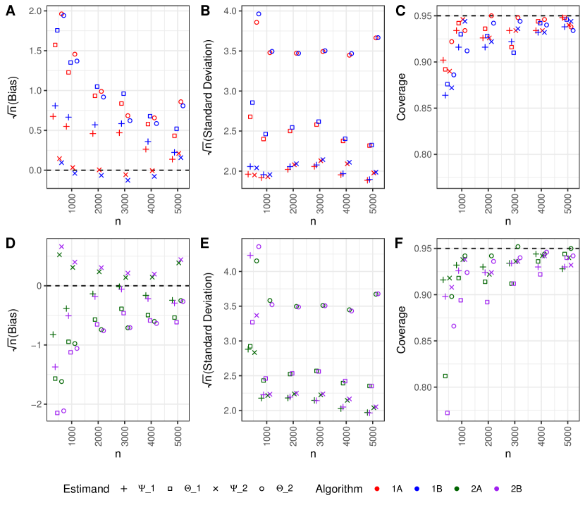
Figure 1: Bias (A, D), empirical standard deviation (B, E) and coverage (C, F) for estimators from DGP 1. Dashed lines indicate zero bias, and nominal 95% CI coverage. For readability, a small amount of ‘jitter’ has been added to the sample size, $n$. In order to present scaled and unscaled TE-VIMs together, the standard deviation and bias of scaled TE-VIMs has been multiplied by the true VTE. Note that the bias and variance scales differ between sub-plots A,B and D,E.

4 Applied example: AIDS clinical trial

The AIDS Clinical Trials Group Protocol 175 (ACTG175) (Hammer et al.,, 1996), considers 2139 HIV patients with CD4 T-cell count between 200 and 500$mm^{-3}$. Patients were randomised to 4 treatment groups: (i) zidovudine (ZDV) monotherapy, (ii) ZDV+didanosine (ddI), (iii) ZDV+zalcitabine, and (iv) ddI monotherapy. We compare groups (iv) and (ii), represented by $A=0,1$, with 561 and 522 patients respectively. We consider CD4 count at 20±5 weeks as a continuous outcome, $Y$, and 12 baseline covariates, 5 continuous: age, weight, Karnofsky score, CD4 count, CD8 count; and 7 binary: sex, homosexual activity (y/n), race (white/non-white), symptomatic status (symptomatic/asymptomatic), intravenous drug use history(y/n), hemophilia (y/n), and antiretroviral history (experienced/naive). Data is available from the speff2trial R package.

TE-VIMs for each covariates were estimated using all algorithms with $K=10$ folds (around 10 folds is typical for cross-fitting procedures). A constant propensity score of $522/1083\approx 0.48$ was used, since treatment is randomized. Fitted models for the outcome and CATEs were obtained using the ‘discrete’ Super Learner (van der Laan et al.,, 2007), an ensemble learning method, which selects the regression algorithm in a ‘learner library’ that minimises some cross-validated loss. We used the SuperLearner R package implementation of this algorithm with 10 cross-validation folds, mean-squared-error loss, and a learner library containing various routines (glm, glmnet, gam, xgboost, ranger).

AIPW estimates of the ATE using pseudo-outcomes from Algorithms 1, 2A, and 2B were similar, respectively: 28.2$mm^{-3}$ (CI: 14.0, 42.3; p$<$0.01); 28.4$mm^{-3}$ (CI: 13.8, 42.9; p$<$0.01); 27.9$mm^{-3}$ (CI: 13.3, 42.5; p$<$0.01), where all CIs are reported at 95% significance and p-values are of Wald type. VTE estimates differed substantially between algorithms with/ without cross-fitting. With Algorithms 1A and 1B returning estimates: 3100$mm^{-6}$ (CI: 1410, 4790; p$<$0.01) and 3600$mm^{-6}$ (CI: 1810, 5380; p$<$0.01), and for Algorithms 2A and 2B: 1260$mm^{-6}$ (CI: -425, 2940; p$=$0.14) and 1250$mm^{-6}$ (CI: -580, 3080; p$=$0.18). It is helpful to also consider the square root of the VTE estimates, which is on the same scale as the ATE. These are 55.7, 60.0, 35.5, and 35.3$mm^{-3}$ for Algorithms 1A, 1B, 2A and 2B respectively. Based on the VTE CIs from Algorithms 2A and 2B, low treatment effect heterogeneity is a concern in this analysis.

Figures 2 and 3 show unscaled and scaled TE-VIM estimates using the LOO and KOI modes. All Algorithms rank CD4 count and homosexual activity as the most important covariates, with CD8 count also appearing in the two top ranked covariates for Algorithm 2B under the KOI mode. We also observe that standard errors are small for unimportant covariates, as expected due to the importance testing issues in Section 2.3.2.

Figure 2: TE-VIM estimates $\hat{\Theta}_{s}$ from the ACTG175 study using each of the proposed Algorithms. Error bars indicate 95% CIs. In each plot, covariates are sorted according to their TE-VIM point estimate. Dashed lines indicate no importance. For the KOI mode, the TE-VIM represents the importance of the complement variable set, i.e. low-values denote high-importance of the KOI covariate.

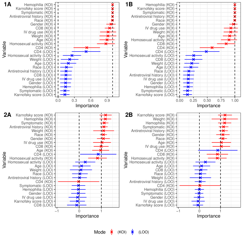
Figure 3: Scaled TE-VIM estimates $\hat{\Psi}_{s}$ from the ACTG175 study using each of the proposed Algorithms. Error bars indicate 95% CIs. In each plot, covariates are sorted according to their TE-VIM point estimate. Dashed lines indicate the $[0,1]$ support of the scaled TE-VIM. For the KOI mode, the TE-VIM represents the importance of the complement variable set, i.e. low-values denote high-importance of the KOI covariate.

5 Related work and extensions

Here we discuss related work on VIMs for the OTR, and extensions of the proposed TE-VIMs to continuous treatments. Further discussion on alternative treatment effect scales, linear CATE projections (Boileau et al.,, 2022), and treatment effect cumulative distribution functions (Levy and van der Laan,, 2018) can be found in Appendix D.

5.1 Optimal treatment rule - VIMs

Whilst TE-VIMs capture the importance of variable subsets in explaining the CATE, this should not be confused with the importance of those variables in contributing to the OTR. For instance, a covariate could be important in explaining the magnitude of the CATE, but unimportant in determining the effect direction, and vice-versa. From a policy learning perspective, it may be more pertinent to investigate the importance of variable subsets in explaining the OTR, $d(\bm{x})\equiv\mathbb{I}\{\tau(\bm{x})>0\}$, where $\mathbb{I}(.)$ denotes an indicator function and we assume w.l.o.g. that a more positive outcome is preferred. The current approach might be extended by considering an OTR-VIM estimand, $\Gamma_{s}\equiv E[\mathrm{var}\{d(\bm{X})|\bm{X}_{-s}\}]=E[d_{s}(\bm{X})\{1-d_{s}(\bm{X})\}]$ where $d_{s}(\bm{x})\equiv E\{d(\bm{X})|\bm{X}_{-s}=\bm{x}_{-s}\}=Pr\{\tau(\bm{X})>0|\bm{X}_{-s}=\bm{x}_{-s}\}$. Note that $d(\bm{X})\in\{0,1\}$ and $d_{s}(\bm{X})\in[0,1]$. We argue that $\Gamma_{s}\in[0,0.25]$ is analogous to $\Theta_{s}$ and $\Omega_{s}$, with the OTR $d(\bm{X})$ used in place of $\tau(\bm{X})$ and $\mu(\bm{X})$ respectively. Alternatively, one might determine variable importance using a classification loss function (logistic loss, AUC, …), or else Williamson et al., 2021b propose OTR-VIMs based on the estimand, $\Gamma^{*}_{s}\equiv E\{\mu(d(\bm{X}),\bm{X})-\mu(d^{*}_{s}(\bm{X}),\bm{X})\}=E\left[\tau(\bm{X})\{d(\bm{X})-d^{*}_{s}(\bm{X})\}\right]\geq 0$ where $d^{*}_{s}(\bm{x})\equiv\mathbb{I}\{\tau_{s}(\bm{x})>0\}$ is the OTR given $\bm{X}_{-s}$. Unlike TE-VIMs, $\Gamma_{s}$ and $\Gamma^{*}_{s}$ are not pathwise differentiable, which complicates inference, hence estimators for $\Gamma^{*}_{s}$ typically treat the OTR as known (Luedtke and van der Laan,, 2016).

5.2 Continuous treatments

Continuous analogues of the CATE based on linear model projections are proposed by Hines et al., (2023). In particular, $\lambda(\bm{x})\equiv\mathrm{cov}(A,Y|\bm{X}=\bm{x})/\mathrm{var}(A|\bm{X}=\bm{x})$ is well defined when $A$ is continuous, and identifies the CATE under standard causal assumptions (consistency, positivity, exchangeability) when $A$ is binary. Appealing to the loss $f\mapsto||\lambda(\bm{X})-f(\bm{X})||^{2}$, one might extend the ATE, VTE, and TE-VIMs to continuous exposures using the estimands: $E\{\lambda(\bm{X})\}$, $\mathrm{var}\{\lambda(\bm{X})\}$, and $E[\mathrm{var}\{\lambda(\bm{X})|\bm{X}_{-s}\}]/\mathrm{var}\{\lambda(\bm{X})\}$, which identify their CATE counterparts when $A$ is binary. ICs for these estimands are obtained by replacing the pseudo-outcome $\varphi(\bm{z})$ with

$$\left[y-\mu(\bm{x})-\lambda(\bm{x})\{a-\pi(\bm{x})\}\right]\frac{a-\pi(\bm{x})}{\mathrm{var}(A|\bm{X}=\bm{x})}+\lambda(\bm{x})$$

which reduces to $\varphi(\bm{z})$ when $A$ is binary. See Appendix D.8 for details.

6 Conclusion

We propose TE-VIMs, which extend the VIM framework of Williamson et al., 2021b to the CATE. These have immediate applications to observational and clinical trial analyses, and provide insight into scientific questions related to treatment effect heterogeneity. Our methods complement VTE analysis, which quantifies treatment effect heterogeneity (Levy et al.,, 2021). We derive efficient estimators that are amenable to data-adaptive estimation of working models. These are broadly applicable, since they are not tied to specific regression algorithms, unlike existing proposals based on causal random forests (Athey et al.,, 2019). We recommend that TE-VIM inference is incorporated into treatment effect analyses, where primary interest is in inferring the ATE and VTE. We recommend that VTE inference forms part of a primary analysis, since the ATE and VTE may be used to bound the marginal probability of adverse CATEs (see Appendix D.7), and since it is possible that the ATE is zero, but some individuals experience large CATEs. One may then infer TE-VIMs in a secondary analysis, when large treatment effect heterogeneity cannot be ruled out, since TE-VIM estimands are not of scientific interest when there is little heterogeneity to account for. We connect our estimators to regression-VIMs via an interpretation in terms of pseudo-outcomes (Kennedy,, 2020). This approach may generalise to other estimands, where analogous pseudo-outcomes can be derived, as in Section 5.2.

Appendix A Derivation of Efficient Influence Curve

We adopt the IC derivation formalism given in Hines et al., (2022). Specifically we let $P_{0}$ denote the true distribution of $(Y,A,\bm{X})$ and let $\tilde{P}$ denote a point mass at $(\tilde{y},\tilde{a},\tilde{\bm{x}})$. We further denote the parametric submodel $P_{t}=t\tilde{P}+(1-t)P_{0}$ where $t\in[0,1]$ is a scalar parameter, and we let $\partial_{t}$ denote an operator such that for some function of $f(t)$, $\partial_{t}f(t)\equiv\frac{df(t)}{dt}|_{t=0}$.

Our goal is to derive an IC for $L^{*}_{P_{0}}\{h\}\equiv E_{P_{0}}[\{\tau(\bm{X})-h(\bm{X})\}^{2}]$, for a known function $h:\mathbb{R}^{p}\mapsto\mathbb{R}$, which we will connect to ICs for $\Theta_{s}$ and $\Psi_{s}$.

We make use of the following lemma, which we demonstrate later in the proof. Letting $g_{P}(X)$ denote some functional of $P$, then

$$\partial_{t}E_{P_{t}}\{g_{P_{t}}(\bm{X})|\bm{X}_{-s}=x_{-s}\} =\frac{\tilde{f}(\bm{x}_{-s})}{f(\bm{x}_{-s})}\left[g_{P_{0}}(\tilde{\bm{x}})-E_{P}\{g_{P_{0}}(\bm{X})|\bm{X}_{-s}=\bm{x}_{-s}\}\right]$$ (4)

$$+E_{P_{0}}\{\partial_{t}g_{P_{t}}(\bm{X})|\bm{X}_{-s}=\bm{x}_{-s}\}$$

where $\tilde{f}(.)$ and $f(.)$ denote the marginal ‘densities’ of $\bm{X}_{-s}$ under $\tilde{P}$ and $P_{0}$ respectively, which are w.l.o.g. absolutely continuous w.r.t. to a dominating measure. In practice this expression means that for discrete $\bm{X}_{-s}$ then $f(.)$ is a probability mass function and $\tilde{f}(.)$ is an indicator function. Similarly for continuous $\bm{X}_{-s}$ then $f(.)$ is a probability density function and $\tilde{f}(.)$ is a Dirac delta function. In both cases $\tilde{f}(\bm{x}_{-s})$ is a probability point mass, which is zero when $\tilde{\bm{x}}_{-s}\neq\bm{x}_{-s}$.

It follows immediately from (4) that,

$$\partial_{t}E_{P_{t}}\{g_{P_{t}}(\bm{X})\} =g_{P_{0}}(\tilde{\bm{x}})-E_{P_{0}}\{g_{P_{0}}(\bm{X})\}+E_{P_{0}}\{\partial_{t}g_{P_{t}}(\bm{X})\}$$ (5)

For the function $g_{P_{t}}(\bm{x})=\{\tau_{t}(\bm{x})-h(\bm{x})\}^{2}$, where $\tau_{t}(\bm{x})$ represents $\tau(\bm{x})$ under $P_{t}$, we obtain

$$\partial_{t}L^{*}_{P_{t}}\{h\}=\{\tau(\tilde{\bm{x}})-h(\tilde{\bm{x}})\}^{2}-L^{*}_{P_{0}}\{h\}+2E_{P_{0}}[\{\tau(\bm{x})-h(\bm{x})\}\partial_{t}\tau_{t}(\bm{x})]$$

we use (4) and the fact that $\tau(\bm{x})=\mu(1,\bm{x})-\mu(0,\bm{x})$ to show that,

$$\partial_{t}\tau_{t}(\bm{x}) =\frac{\tilde{f}(\bm{x})}{f(\bm{x})}\{\tilde{y}-\mu(\tilde{a},\bm{x})\}\frac{\tilde{a}-\pi(\bm{x})}{\pi(\bm{x})\{1-\pi(\bm{x})\}}$$

hence we obtain the IC

$$\partial_{t}L^{*}_{P_{t}}\{h\} =\{\tau(\tilde{\bm{x}})-h(\tilde{\bm{x}})\}^{2}-L^{*}_{P_{0}}\{h\}+2\{\tau(\tilde{\bm{x}})-h(\tilde{\bm{x}})\}\{\tilde{y}-\mu(\tilde{a},\tilde{\bm{x}})\}\frac{\tilde{a}-\pi(\tilde{\bm{x}})}{\pi(\tilde{\bm{x}})\{1-\pi(\tilde{\bm{x}})\}}$$

$$=\{\tau(\tilde{\bm{x}})-h(\tilde{\bm{x}})\}^{2}-L^{*}_{P_{0}}\{h\}+2\{\tau(\tilde{\bm{x}})-h(\tilde{\bm{x}})\}\{\varphi(\tilde{\bm{z}})-\tau(\tilde{\bm{x}})\}$$

Completing the square of the expression above gives

$$\partial_{t}L^{*}_{P_{t}}\{h\} =\{\varphi(\tilde{\bm{z}})-h(\tilde{\bm{x}})\}^{2}-\{\varphi(\tilde{\bm{z}})-\tau(\tilde{\bm{x}})\}^{2}-L^{*}_{P_{0}}\{h\}$$

When replicating this proof, it is useful to note that for an arbitrary function $w(\bm{x})$

$$E_{P_{0}}\left\{\frac{\tilde{f}(\bm{X})}{f(\bm{X})}w(\bm{X})\right\} =w(\tilde{\bm{x}})$$

A.1 Proof of Lemma in (4)

To demonstrate (4) we write the lefthand side as

$$\partial_{t}\int g_{P_{t}}(\bm{x}^{*})dP_{t,\bm{X}_{s}|\bm{x}_{-s}}(\bm{x}^{*}_{s}) =\int g_{P}(\bm{x}^{*})\partial_{t}dP_{t,\bm{X}_{s}|\bm{x}_{-s}}(\bm{x}^{*}_{s})+\int\{\partial_{t}g_{P_{t}}(\bm{x}^{*})\}dP_{\bm{X}_{s}|\bm{x}_{-s}}(\bm{x}^{*}_{s})$$

where $dP_{t,\bm{X}_{s}|\bm{x}_{-s}}(.)$ is the conditional distribution of $\bm{X}_{s}$ given $\bm{X}_{-s}=\bm{x}_{-s}$ under the parametric submodel and $\bm{x}^{*}_{-s}=\bm{x}_{-s}$. The second integral on the righthand side recovers the final term in (4). Hence the lemma follows once we show that

$$\partial_{t}dP_{t,\bm{X}_{s}|\bm{x}_{-s}}(\bm{x}^{*}_{s})=\frac{\tilde{f}(\bm{x}_{-s})}{f(\bm{x}_{-s})}\{d\tilde{P}_{\bm{X}_{s}}(\bm{x}^{*}_{s})-dP_{\bm{X}_{s}|\bm{x}_{-s}}(\bm{x}^{*}_{s})\}$$

To do so, let $\mu$ denote a dominating measure and write

$$dP_{t,\bm{X}_{s}|\bm{x}_{-s}}(\bm{x}^{*}_{s}) =f_{t,\bm{X}_{s}|\bm{x}_{-s}}(\bm{x}^{*}_{s})d\mu(\bm{x}^{*}_{s})$$

$$=\frac{f_{t,\bm{X}}(\bm{x}^{*})}{f_{t,\bm{X}_{-s}}(\bm{x}_{-s})}d\mu(\bm{x}^{*}_{s})$$

where $f_{t,\bm{X}}(.)$ and $f_{t,\bm{X}_{-s}}(.)$ denote the marginal densities of $\bm{X}$ and $\bm{X}_{-s}$ under the parametric submodel, $P_{t}$, i.e. they are the Radon-Nikodym derivatives w.r.t. $\mu$. Applying the quotient rule, we obtain

$$\partial_{t}dP_{t,\bm{X}_{s}|\bm{x}_{-s}}(\bm{x}^{*}_{s}) =\frac{1}{f_{\bm{X}_{-s}}(\bm{x}_{-s})}\left[\partial_{t}f_{t,\bm{X}}(\bm{x}^{*})-\frac{f_{\bm{X}}(\bm{x}^{*})}{f_{\bm{X}_{-s}}(\bm{x}_{-s})}\partial_{t}f_{t,\bm{X}_{-s}}(\bm{x}_{-s})\right]d\mu(\bm{x}^{*}_{s})$$

We now evaluate the derivative parts. Since $\partial_{t}P_{t}=\tilde{P}-P$, the marginal density derivatives will have a similar structure, as shown in the first expression below, where $f_{\bm{X}}(.)$ and $\tilde{f}_{\bm{X}}(.)$ denote marginal densities of $\bm{X}$ under $\tilde{P}$ and $P$, with likewise for $\bm{X}_{-s}$

$$\partial_{t}dP_{t,\bm{X}_{s}|\bm{x}_{-s}}(\bm{x}^{*}) =\frac{1}{f_{\bm{X}_{-s}}(\bm{x}_{-s})}\left[\{\tilde{f}_{\bm{X}}(\bm{x}^{*})-f_{\bm{X}}(\bm{x}^{*})\}-\frac{f_{\bm{X}}(\bm{x}^{*})}{f_{\bm{X}_{-s}}(\bm{x}_{-s})}\{\tilde{f}_{\bm{X}_{-s}}(\bm{x}_{-s})-f_{\bm{X}_{-s}}(\bm{x}_{-s})\}\right]d\mu(\bm{x}^{*}_{s})$$

Since $\tilde{P}$ is a point mass, $\tilde{f}_{\bm{X}}(\bm{x}^{*})=\tilde{f}_{\bm{X}_{s}}(\bm{x}^{*}_{s})\tilde{f}_{\bm{X}_{-s}}(\bm{x}^{*}_{-s})$. Also $\bm{x}^{*}_{-s}=\bm{x}_{-s}$ hence,

$$\partial_{t}dP_{t,\bm{X}_{s}|\bm{x}_{-s}}(\bm{x}^{*}) =\frac{\tilde{f}_{\bm{X}_{-s}}(\bm{x}_{-s})}{f_{\bm{X}_{-s}}(\bm{x}_{-s})}\left[\tilde{f}_{\bm{X}_{s}}(\bm{x}^{*}_{s})-\frac{f_{\bm{X}}(\bm{x}^{*})}{f_{\bm{X}_{-s}}(\bm{x}_{-s})}\right]d\mu(\bm{x}^{*}_{s})$$

$$=\frac{\tilde{f}_{\bm{X}_{-s}}(\bm{x}_{-s})}{f_{\bm{X}_{-s}}(\bm{x}_{-s})}\left[\tilde{f}_{\bm{X}_{s}}(\bm{x}^{*}_{s})-f_{\bm{X}_{s}|\bm{x}_{-s}}(\bm{x}^{*}_{s})\right]d\mu(\bm{x}^{*}_{s})$$

Thus, the result follows.

Appendix B Estimator Asymptotic Distributions

In this Appendix we use a common empirical processes notation, where we define linear operators $P_{0}$ and $\mathbb{P}_{n}$ such that for some function $h(\bm{Z})$, $P_{0}\{h(\bm{Z})\}\equiv E\{h(\bm{Z})\}$ and $\mathbb{P}_{n}\{h(\bm{Z})\}\equiv n^{-1}\sum_{i=1}^{n}h(\bm{z}_{i})$. To simplify notation we also largely omit function arguments, for example $\tau=\tau(\bm{X})$ with similar for $\hat{\tau},\tau_{s},\hat{\tau}_{s},\pi,\hat{\pi},\hat{\varphi}$.

B.1 Proof of Theorem 1

Define

$$\hat{\varphi}(\bm{z}) \equiv\{y-\hat{\mu}(a,\bm{x})\}\frac{a-\hat{\pi}(\bm{x})}{\hat{\pi}(\bm{x})\{1-\hat{\pi}(\bm{x})\}}+\hat{\mu}(1,\bm{x})-\hat{\mu}(0,\bm{x})$$

$$\hat{\phi}_{s}(\bm{z}) \equiv\{\hat{\varphi}(\bm{z})-\hat{\tau}_{s}(\bm{x})\}^{2}-\{\hat{\varphi}(\bm{z})-\hat{\tau}(\bm{x})\}^{2}-\hat{\Theta}_{s}^{0}$$

where $\hat{\Theta}_{s}^{0}$ is an initial estimate of $\Theta_{s}$. Without making any restrictions we write

$$\hat{\Theta}_{s}-\Theta_{s} =(\mathbb{P}_{n}-P_{0})\{\phi_{s}(\bm{Z})\}+R_{n}+H_{n}$$ (6)

$$\hat{\Theta}_{s} \equiv\hat{\Theta}_{s}^{0}+\mathbb{P}_{n}\{\hat{\phi}_{s}(\bm{Z})\}$$ (7)

$$R_{n} \equiv\hat{\Theta}_{s}^{0}-\Theta_{s}+P_{0}\{\hat{\phi}_{s}(\bm{Z})\}$$ (8)

$$H_{n} \equiv(\mathbb{P}_{n}-P_{0})\{\hat{\phi}_{s}(\bm{Z})-\phi_{s}(\bm{Z})\}.$$ (9)

We will show that the remainder therm $R_{n}=o_{P}(n^{-1/2})$ and the empirical process term $H_{n}=o_{P}(n^{-1/2})$, and hence the result follows since $P_{0}\{\phi_{\psi}(\bm{Z})\}=0$.

B.2 The remainder term

Evaluating the remainder $R_{n}=E\{\hat{\phi}_{s}(\bm{Z})+\hat{\Theta}_{s}^{0}-\Theta_{s}\}$ gives

$$R_{n} =E\left[\{\hat{\varphi}-\hat{\tau}_{s}\}^{2}-\{\hat{\varphi}-\hat{\tau}\}^{2}-\{\tau-\tau_{s}\}^{2}\right]$$

where we have used the fact that $\Theta_{s}=E[\{\tau-\tau_{s}\}^{2}]$. By algebraic manipulation, we write

$$R_{n} =E\left[\{\hat{\tau}-\hat{\tau}_{s}\}^{2}-\{\tau-\tau_{s}\}^{2}+2\{\hat{\tau}-\hat{\tau}_{s}\}\{\hat{\varphi}-\hat{\tau}\}\right]$$

We then use the identity,

$$E\left[\{\hat{\tau}-\hat{\tau}_{s}\}^{2}-\{\tau-\tau_{s}\}^{2}\right] =E\left[\{\tau_{s}-\hat{\tau}_{s}\}^{2}-\{\tau-\hat{\tau}\}^{2}+2\{\hat{\tau}-\hat{\tau}_{s}\}\{\hat{\tau}-\tau\}\right]$$

to rewrite the remainder term as the sum of two error terms,

$$R_{n} =E\left[\{\hat{\tau}-\hat{\tau}_{s}\}^{2}-\{\tau-\tau_{s}\}^{2}+2\{\hat{\tau}-\hat{\tau}_{s}\}\{\hat{\varphi}-\hat{\tau}\}\right]$$

$$=E\left[\{\tau_{s}-\hat{\tau}_{s}\}^{2}-\{\tau-\hat{\tau}\}^{2}+2\{\hat{\tau}-\hat{\tau}_{s}\}\{\hat{\tau}-\tau\}+2\{\hat{\tau}-\hat{\tau}_{s}\}\{\hat{\varphi}-\hat{\tau}\}\right]$$

$$=E\left[\{\tau_{s}-\hat{\tau}_{s}\}^{2}-\{\tau-\hat{\tau}\}^{2}+2\{\hat{\tau}-\hat{\tau}_{s}\}\{\hat{\varphi}-\tau\}\right]$$

$$=\underbrace{E\left[\{\tau_{s}-\hat{\tau}_{s}\}^{2}-\{\tau-\hat{\tau}\}^{2}\right]}_{\text{CATE error}}+\underbrace{2E\left[\{\hat{\tau}-\hat{\tau}_{s}\}r\right]}_{\text{Pseudo-outcome error}}$$

where $r=r(\bm{X})$ is defined by $r(\bm{x})\equiv E\left[\hat{\varphi}|\bm{X}=\bm{x}\right]-\tau(\bm{x})$, which represents a pseudo-outcome error in the sense that $r(\bm{x})=E\left[\hat{\varphi}-\varphi|\bm{X}=\bm{x}\right]$. Splitting the remainder in to two error terms allows us to consider that the CATE error is $o_{P}(n^{-1/2})$ when (A2) holds. For the pseudo-outcome error we use the Cauchy-Schwarz inequality to show that

$$E\left[\{\hat{\tau}-\hat{\tau}_{s}\}r\right]^{2} \leq E\left[\{\hat{\tau}-\hat{\tau}_{s}\}^{2}\right]E\left[r^{2}\right]\leq\delta E\left[r^{2}\right]$$

Hence the pseudo-outcome error term is $o_{P}(n^{-1/2})$ if $r$ is $o_{P}(n^{-1/2})$. By iterated expectation

$$r(\bm{x}) =\left\{\frac{\pi(\bm{x})}{\hat{\pi}(\bm{x})}-1\right\}\left\{\mu(1,\bm{x})-\hat{\mu}(1,\bm{x})\right\}-\left\{\frac{1-\pi(\bm{x})}{1-\hat{\pi}(\bm{x})}-1\right\}\left\{\mu(0,\bm{x})-\hat{\mu}(0,\bm{x})\right\}$$

Using the inequality $(a+b)^{2}\leq 2(a^{2}+b^{2})$ then

$$r^{2}(\bm{x}) \leq 2\left\{\frac{\pi(\bm{x})}{\hat{\pi}(\bm{x})}-1\right\}^{2}\left\{\mu(1,\bm{x})-\hat{\mu}(1,\bm{x})\right\}^{2}+2\left\{\frac{1-\pi(\bm{x})}{1-\hat{\pi}(\bm{x})}-1\right\}^{2}\left\{\mu(0,\bm{x})-\hat{\mu}(0,\bm{x})\right\}^{2}$$

$$\leq\left(\frac{2}{\epsilon^{2}}\right)\left\{\pi(\bm{x})-\hat{\pi}(\bm{x})\right\}^{2}\left[\left\{\mu(1,\bm{x})-\hat{\mu}(1,\bm{x})\right\}^{2}+\left\{\mu(0,\bm{x})-\hat{\mu}(0,\bm{x})\right\}^{2}\right]$$

with the second inequality follows since $\hat{\pi}\in(\epsilon,1-\epsilon)$. The final expression above is $o_{P}(n^{-1})$ under (A1), which completes the proof that $R_{n}$ itself is $o_{P}(n^{-1/2})$.

B.3 The empirical process term

First write the empirical process term as the sum

$$H_{n} =(\mathbb{P}_{n}-P_{0})\{\Theta_{s}-\hat{\Theta}_{s}^{0}\}$$

$$+2(\mathbb{P}_{n}-P_{0})\{(\hat{\varphi}-\varphi)(\hat{\tau}-\hat{\tau}_{s})\}$$

$$+(\mathbb{P}_{n}-P_{0})\{(\varphi-\hat{\tau}_{s})^{2}-(\varphi-\tau_{s})^{2}\}$$

$$-(\mathbb{P}_{n}-P_{0})\{(\varphi-\hat{\tau})^{2}-(\varphi-\tau)^{2}\}$$

Note that the first term is zero since $(\mathbb{P}_{n}-P_{0})\{\Theta_{s}-\hat{\Theta}_{s}^{0}\}=(\Theta_{s}-\hat{\Theta}_{s}^{0})(\mathbb{P}_{n}-P_{0})\{1\}=0$. When the Donsker condition holds, then, by Lemma 19.24 of van der Vaart, (1998) , the second term is $o_{P}(n^{-1/2})$ provided (i) that $E\{(\hat{\varphi}-\varphi)^{2}(\hat{\tau}-\hat{\tau}_{s})^{2}\}=o_{p}(1)$, the third term is $o_{P}(n^{-1/2})$ provided (ii) that $E\left[\left\{(\varphi-\hat{\tau}_{s})^{2}-(\varphi-\tau_{s})^{2}\right\}^{2}\right]=o_{p}(1)$, and the fourth term is $o_{P}(n^{-1/2})$ provided (iii) that $E\left[\left\{(\varphi-\hat{\tau})^{2}-(\varphi-\tau)^{2}\right\}^{2}\right]=o_{p}(1)$. Similarly, under sample splitting then by Chebyshev’s inequality, (i), (ii), and (iii) are also sufficient conditions for $H_{n}$ to be $o_{P}(n^{-1/2})$. We will examine these conditions in reverse order.

For (iii) we write

$$(\varphi-\hat{\tau})^{2}-(\varphi-\tau)^{2} =2(\varphi-\tau)(\tau-\hat{\tau})+(\tau-\hat{\tau})^{2}$$

$$E\left[\left\{(\varphi-\hat{\tau})^{2}-(\varphi-\tau)^{2}\right\}^{2}|\bm{X}\right] =4\mathrm{var}(\varphi|\bm{X})(\tau-\hat{\tau})^{2}+(\tau-\hat{\tau})^{4}$$

Since $\hat{\tau}$ is consistent, and $\mathrm{var}(\varphi|\bm{X})<K$ then (iii) holds. Also since $\hat{\tau}_{s}$ is consistent then (ii) holds in the same way. For (i) we write

$$E\{(\hat{\varphi}-\varphi)^{2}(\hat{\tau}-\hat{\tau}_{s})^{2}\}\leq\delta E\{(\hat{\varphi}-\varphi)^{2}\}$$

and we remark that $E\{(\hat{\varphi}-\varphi)^{2}\}$ is the empirical process term which appears in analogous derivations for average treatment effect estimators. Therefore, in view of Theorem 5.1 of Chernozhukov et al., (2018), this term also converges to zero when (A1) holds, $\hat{\pi}\in(\epsilon,1-\epsilon)$, and $\mathrm{var}(Y|\bm{X})<K$.

Thus $H_{n}=o_{P}(n^{-1/2})$ which completes the proof.

B.4 Proof of Theorem 2

Suppose we have two regular asymptotically linear estimators

$$\hat{\Theta}_{s}-\Theta_{s} =\mathbb{P}_{n}\{\phi_{s}(\bm{Z})\}+o_{p}(n^{-1/2})$$ (10)

$$\hat{\Theta}_{p}-\Theta_{p} =\mathbb{P}_{n}\{\phi_{p}(\bm{Z})\}+o_{p}(n^{-1/2})$$ (11)

It follows by algebraic manipulations that

$$n^{1/2}(\hat{\Psi}_{s}-\Psi_{s}) =\frac{\Theta_{p}}{\hat{\Theta}_{p}}\left[n^{1/2}\mathbb{P}_{n}\{\Phi_{s}(\bm{Z})\}+o_{p}(1)\right]$$

where $\Phi_{s}(z)=\{\phi_{s}(z)-\Psi_{s}\phi_{p}(z)\}/\Theta_{p}$ is the IC of $\Psi_{s}$. By Slutsky’s Theorem and the fact that $\hat{\Theta}_{p}/\Theta_{p}$ converges to 1 in probability

$$\lim_{n\to\infty}n^{1/2}(\hat{\Psi}_{s}-\Psi_{s}) =\lim_{n\to\infty}n^{1/2}\mathbb{P}_{n}\{\Phi_{s}(\bm{Z})\}$$

which gives the desired result due to the central limit theorem. We note that this set up is quite general when one considers estimands which are written as the ratio of two other estimands, such as $\Psi_{s}$ in the present context.

Clearly (10) follows by Theorem 1. We must therefore check that (11) also holds.

Most of the steps in the Proof of Theorem 1 can be applied directly to $\Theta_{p}$. When decomposing the empirical process term, however, we are left with the term

$$(\mathbb{P}_{n}-P_{0})\{(\varphi-\hat{\tau}_{p}^{*})^{2}-(\varphi-\tau_{p})^{2}\}$$

in place of the corresponding term involving $\tau_{s}$. Since $\tau_{p}$ and $\hat{\tau}_{p}^{*}$ are constant this term reduces to

$$(\hat{\tau}_{p}^{*}-\tau_{p})^{2}-2(\hat{\tau}_{p}^{*}-\tau_{p})(\mathbb{P}_{n}-P_{0})\{\varphi\}$$

Next we note that the conditions of Theorem 1 imply that the AIPW is a RAL estimator of the ATE

$$\hat{\tau}_{p}^{*}-\tau_{p}=\mathbb{P}_{n}\{\varphi-\tau_{p}\}+o_{P}(n^{-1/2})$$

See e.g. Theorem 5.1 of Chernozhukov et al., (2018). Also, $(\mathbb{P}_{n}-P_{0})\{\varphi\}\overset{p}{\to}0$ by the weak law of large numbers. Therefore this term in the empirical process term decomposition will be $o_{P}(n^{-1/2})$, which completes the proof.

Appendix C Additional plots for simulation results

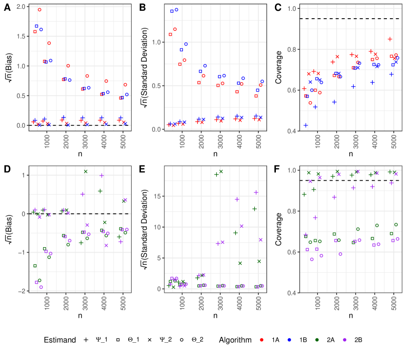
Figure 4: Bias (A, D), empirical standard deviation (B, E) and coverage (C, F) for estimators from DGP 2. Dashed lines indicate zero bias, and nominal 95% CI coverage. For readability, a small amount of ‘jitter’ has been added to the sample size, $n$. In order to present scaled and unscaled TE-VIMs together, the standard deviation and bias of scaled TE-VIMs has been multiplied by the true VTE. Note that the bias and variance scales differ between sub-plots A,B and D,E.

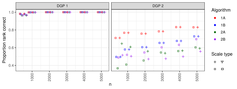
Figure 5: Empirical probability that (scaled) TE-VIMs recover the correct importance ranking for DGPs 1 and 2. For readability, a small amount of ‘jitter’ has been added to $n$.

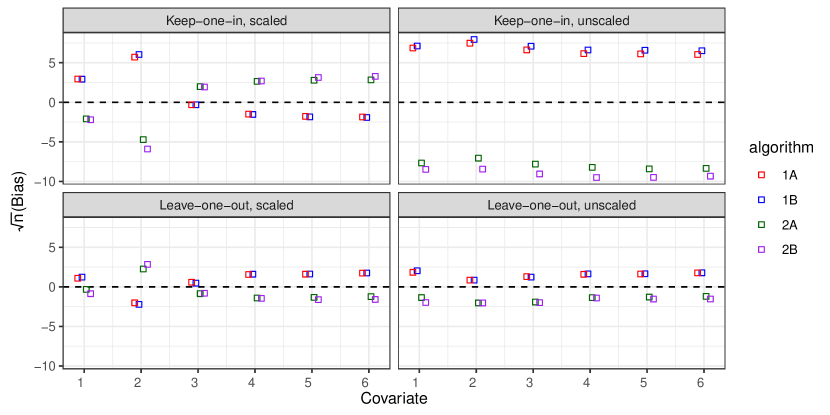
Figure 6: Empirical bias for estimators from DGP 3. Dashed lines indicate zero bias. In order to present scaled and unscaled TE-VIMs together, the bias of scaled TE-VIMs has been multiplied by the true VTE $\Theta_{p}=8$. Here scaled and unscaled refers to estimators of the type $\Psi$ and $\Theta$ respectively.

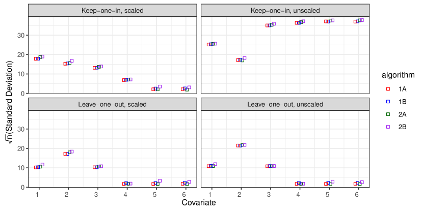
Figure 7: Empirical standard deviation of estimators from DGP 3. Dashed lines indicate zero bias. In order to present scaled and unscaled TE-VIMs together, the standard deviation of scaled TE-VIMs has been multiplied by the true VTE $\Theta_{p}=8$. Here scaled and unscaled refers to estimators of the type $\Psi$ and $\Theta$ respectively.

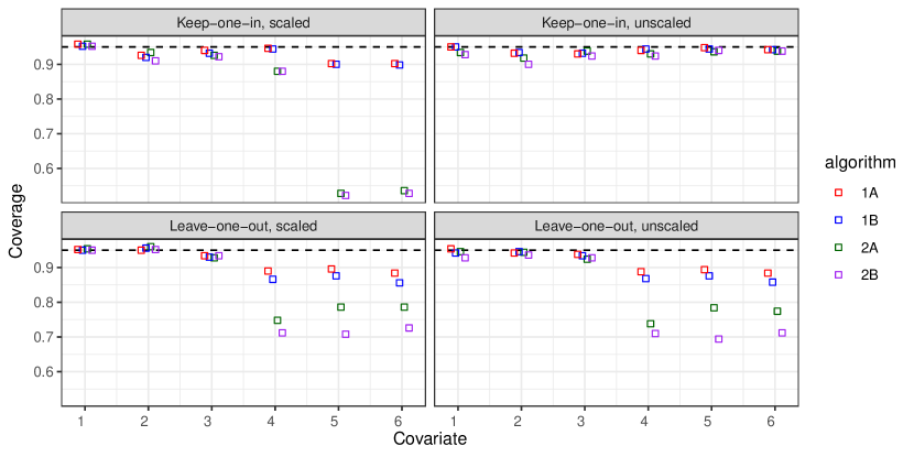
Figure 8: Empirical CI coverage for estimators from DGP 3. Dashed lines indicate nominal 95% CI coverage. Here scaled and unscaled refers to estimators of the type $\Psi$ and $\Theta$ respectively.

Appendix D Additional discussion

D.1 Invariance to transformations

The scaled TE-VIM $\Psi_{s}$ is invariant to linear outcome transformations. To see why, let $\tilde{Y}=bY+k$ and $\tilde{Y}^{a}=bY^{a}+k$ for constants $b\neq 0$ and $k$. Letting superscript tilde to denote the modified values,

$$\tilde{\tau}(x) \equiv E(\tilde{Y}^{1}-\tilde{Y}^{0}|\bm{X}=\bm{x})=b\tau(\bm{x})$$

$$\implies\tilde{\Theta}_{s} \equiv E[\mathrm{var}\{\tilde{\tau}(\bm{X})|\bm{X}_{-s}\}]=b^{2}\Theta_{s}$$

$$\implies\tilde{\Psi}_{s} \equiv\frac{\tilde{\Theta}_{s}}{\tilde{\Theta}_{p}}=\frac{\Theta_{s}}{\Theta_{p}}=\Psi_{s}.$$

Moreover, $\Psi_{s}$ is invariant to invertible component wise mappings of $\bm{X}$. To see why, consider a mapping $g:\mathbb{R}^{p}\mapsto\mathbb{R}^{p}$ such that

$$g(\bm{x})=(g_{1}(x_{1}),...,g_{p}(x_{p}))$$

where $g_{j}:\mathbb{R}\mapsto\mathbb{R}$ is an invertible function for $j\in\{1,...,p\}$. The claim follows since the conditional distribution of $Y$ induced by $\bm{X}_{-s}$ is the same as that induced by $g(\bm{X})_{-s}$. In particular, using superscript tilde to denote a different set of modified values,

$$\tilde{\tau}(g(\bm{x})) \equiv E(Y^{1}-Y^{0}|g(\bm{X})=g(\bm{x}))=\tau(\bm{x})$$

$$\implies\tilde{\Theta}_{s} \equiv E[\mathrm{var}\{\tilde{\tau}(g(\bm{X}))|g(\bm{X})_{-s}\}]=E[\mathrm{var}\{\tau(\bm{X})|g(\bm{X})_{-s}\}]=\Theta_{s}$$

$$\implies\tilde{\Psi}_{s} \equiv\frac{\tilde{\Theta}_{s}}{\tilde{\Theta}_{p}}=\frac{\Theta_{s}}{\Theta_{p}}=\Psi_{s}.$$

D.2 Shapley values

We use the Shapley value definition given by Williamson and Feng, (2020) for an arbitrary value/ loss function. For covariate $j\in\{1,...,p\}$, and letting $\mathcal{P}_{j}$ denote the power set (set of all possible subsets) of $\{1,...,p\}\setminus\{j\}$, we define the TE-VIM Shapley value

$$S_{j}\equiv\sum_{s\in\mathcal{P}_{j}}\frac{1}{p}\binom{p-1}{|s|}^{-1}\{\Theta_{s\cup\{j\}}-\Theta_{s}\}$$

Since $\Theta_{s\cup\{j\}}\geq\Theta_{s}$ for all $s$, then $S_{j}\geq 0$. Also, by construction

$$\Theta_{p}=\sum_{j=1}^{p}S_{j}.$$

D.3 Plug-in estimators

Plug-in estimators for the TE-VIM $\Theta_{s}$ and the scaled TE-VIM $\Psi_{s}$ are non-trivial to construct using estimators for $\tau(\bm{x})$ and $\tau_{s}(\bm{x})$. We illustrate this by considering plug-in estimation of the regression-VIM $\Omega_{s}$ which suffers similar difficulties. Writing the regression-VIM as

$$\Omega_{s}=E\left[\{\mu(\bm{X})-\mu(_{s}\bm{X})\}^{2}\right]$$

Williamson et al., 2021a construct a ‘naive plug-in’ estimator

$$\hat{\Omega}^{0}_{s}=n^{-1}\sum_{i=1}^{n}\{\hat{\mu}(\bm{x}_{i})-\hat{\mu}(_{s}\bm{x}_{i})\}^{2}.$$

However, this estimator is not strictly plug-in in the estimand mapping sense discussed in the main paper. To see why, we write $\Omega_{s}$ in terms of $\mu(\bm{x})$, the distribution of $\bm{X}_{s}$ given $\bm{X}_{-s}$, which we denote by the measure $dP_{0}(\bm{x}_{s}|\bm{x}_{-s})$, and the distribution of $\bm{X}_{-s}$, denoted $dP_{0}(\bm{x}_{s})$,

$$\Omega_{s}=\int\left[\mu(\bm{x})-\left\{\int\mu(\bm{x})\underbrace{dP_{0}(\bm{x}_{s}|\bm{x}_{-s})}_{\text{regression}}\right\}\right]^{2}\underbrace{dP_{0}(\bm{x}_{s}|\bm{x}_{-s})}_{\text{empirical}}dP_{0}(\bm{x}_{s}).$$

Hence, in the estimand definition, the distribution of $\bm{X}_{s}$ given $\bm{X}_{-s}$ appears twice. However, the $\hat{\Omega}^{0}_{s}$ estimator effectively uses, two different (and possibly inconsistent) implicit distributions to approximate $dP_{0}(\bm{x}_{s}|\bm{x}_{-s})$. The first is implied by the regression estimate $\hat{\mu}_{s}(\bm{x})$, whilst the second is implied by the empirical distribution of covariates. In particular, this inconsistency means that there is no guarantee that

$$n^{-1}\sum_{i=1}^{n}\hat{\mu}(\bm{x}_{i})=n^{-1}\sum_{i=1}^{n}\hat{\mu}_{s}(\bm{x}_{i})$$

without additional steps taken to ensure that this identity holds e.g. through targeting (in a TMLE sense) an initial regression estimator of $\hat{\mu}_{s}(\bm{x})$.

We remark that for the Proofs in Appendix B, the exact form of the initial TE-VIM estimator $\hat{\Theta}^{0}_{s}$ does not affect the form of the final estimator $\hat{\Theta}_{s}$, which, can be thought of as a bias-corrected version of $\hat{\Theta}^{0}_{s}$. As such, one could let $\hat{\Theta}^{0}_{s}=n^{-1}\sum_{i=1}^{n}\{\hat{\tau}(\bm{x}_{i})-\hat{\tau}(_{s}\bm{x}_{i})\}^{2}$, though this estimand is also not plug-in for the reasons above.

D.4 TE-VIMs estimation on different scales

The TE-VIM $\Theta_{s}\geq 0$ and the scaled TE-VIM $\Psi_{s}\in[0,1]$ are both bounded, therefore one might want to perform inference on scales which respect these bounds. For instance, one may prefer to treat $\log(\Theta_{s})$ as the target estimand, with the assumption that $\Theta_{s}>0$, or treat $\operatorname*{logit}(\Psi_{s})$ as the target estimand, assuming $\Psi_{s}\in(0,1)$. Here we sketch how one-step bias correction estimators could be constructed for these alternatives, and derive their asymptotic distributions.

First consider that, since the IC represents a pathwise derivatives for $\log(\Theta_{s})$ and $\operatorname*{logit}(\Psi_{s})$ respectively are

$$\frac{\phi_{s}(\bm{Z})}{\Theta_{s}}$$

$$\frac{\Phi_{s}(\bm{Z})}{\Psi_{s}(1-\Psi_{s})}$$

Hence, starting from initial estimators $\hat{\Theta}^{0}_{s}$ and $\hat{\Psi}^{0}_{s}$ one could construct the one-step bias corrected estimators

$$\log(\hat{\Theta}^{0}_{s}) +\frac{n^{-1}\sum_{i=1}^{n}\hat{\phi}_{s}(\bm{z}_{i})}{\hat{\Theta}^{0}_{s}}$$

$$\operatorname*{logit}(\hat{\Psi}^{0}_{s}) +\frac{n^{-1}\sum_{i=1}^{n}\hat{\Phi}_{s}(\bm{z}_{i})}{\hat{\Psi}^{0}_{s}(1-\hat{\Psi}^{0}_{s})}$$

which we rewrite in terms of the estimators in the main text as

$$\log(\hat{\Theta}^{0}_{s}) +\frac{(\hat{\Theta}_{s}-\hat{\Theta}^{0}_{s})}{\hat{\Theta}^{0}_{s}}$$ (12)

$$\operatorname*{logit}(\hat{\Psi}^{0}_{s}) +\frac{\hat{\Theta}_{p}}{\hat{\Theta}_{p}^{0}}\frac{(\hat{\Psi}_{s}-\hat{\Psi}_{s}^{0})}{\hat{\Psi}^{0}_{s}(1-\hat{\Psi}^{0}_{s})}$$ (13)

where, letting $\hat{\Psi}^{0}_{s}=\hat{\Theta}^{0}_{s}/\hat{\Theta}^{0}_{p}$, we have used the fact that

$$n^{-1}\sum_{i=1}^{n}\hat{\Phi}_{s}(\bm{z}_{i}) =\frac{n^{-1}\sum_{i=1}^{n}\hat{\phi}_{s}(\bm{z}_{i})-\hat{\Psi}^{0}_{s}n^{-1}\sum_{i=1}^{n}\hat{\phi}_{p}(\bm{z}_{i})}{\hat{\Theta}_{p}^{0}}$$

$$=\frac{(\hat{\Theta}_{s}-\hat{\Theta}_{s}^{0})-\hat{\Psi}^{0}_{s}(\hat{\Theta}_{p}-\hat{\Theta}_{p}^{0})}{\hat{\Theta}_{p}^{0}}$$

$$=\frac{\hat{\Theta}_{p}}{\hat{\Theta}_{p}^{0}}(\hat{\Psi}_{s}-\hat{\Psi}_{s}^{0})$$

We remark that, unlike the estimators $\hat{\Theta}_{s}$ and $\hat{\Psi}_{s}$, the estimators in (12) and (13) depend on the initial estimators $\hat{\Theta}^{0}_{s}$ and $\hat{\Psi}^{0}_{s}$ in a non-trivial way. We derive asymptotic distributions of these estimators given additional conditions on these initial estimators.

Theorem 3.

Assume the conditions of Theorem 1 hold, $\Theta_{s}>0$, and $(\Theta_{s}-\hat{\Theta}^{0}_{s})/\hat{\Theta}^{0}_{s}=o_{P}(n^{-1/4})$, then the estimator in (12) converges to $\log(\Theta_{s})$ in probability, with a difference that, when multiplied by $n^{1/2}$, converges to a mean-zero normal random variable, with variance $||\phi_{s}(\bm{Z})||^{2}/\Theta_{s}^{2}$.

Proof.

Under the conditions of Theorem 1, then $\hat{\Theta}_{s}$ is regular asymptotically linear, i.e. we can write

$$\hat{\Theta}_{s}=\Theta_{s}+n^{-1}\sum_{i=1}^{n}\phi_{s}(\bm{z}_{i})+o_{P}(n^{-1/2})$$

Hence,

$$\log(\hat{\Theta}^{0}_{s})+\frac{(\hat{\Theta}_{s}-\hat{\Theta}^{0}_{s})}{\hat{\Theta}^{0}_{s}}-\log(\Theta_{s}) =n^{-1}\sum_{i=1}^{n}\frac{\phi_{s}(\bm{z}_{i})}{\hat{\Theta}^{0}_{s}}+\frac{o_{P}(n^{-1/2})}{\hat{\Theta}^{0}_{s}}+\frac{\Theta_{s}-\hat{\Theta}^{0}_{s}}{\hat{\Theta}^{0}_{s}}-\log\left(1+\frac{\Theta_{s}-\hat{\Theta}^{0}_{s}}{\hat{\Theta}^{0}_{s}}\right)$$

Using the Taylor series of $\log(1+x)$

$$=n^{-1}\sum_{i=1}^{n}\frac{\phi_{s}(\bm{z}_{i})}{\hat{\Theta}^{0}_{s}}+\frac{o_{P}(n^{-1/2})}{\hat{\Theta}^{0}_{s}}+\sum_{j=2}^{\infty}\frac{(-1)^{j+1}}{j}\left(\frac{\Theta_{s}-\hat{\Theta}^{0}_{s}}{\hat{\Theta}^{0}_{s}}\right)^{j}$$

$$=\left\{n^{-1}\sum_{i=1}^{n}\frac{\phi_{s}(\bm{z}_{i})}{\Theta_{s}}+\frac{o_{P}(n^{-1/2})}{\Theta_{s}}\right\}(1+\hat{u})+\sum_{j=2}^{\infty}\frac{(-1)^{j+1}\hat{u}^{j}}{j}$$

where $\hat{u}\equiv(\Theta_{s}-\hat{\Theta}^{0}_{s})/\hat{\Theta}^{0}_{s}=o_{P}(n^{-1/4})$ thus

$$\log(\hat{\Theta}^{0}_{s})+\frac{(\hat{\Theta}_{s}-\hat{\Theta}^{0}_{s})}{\hat{\Theta}^{0}_{s}}-\log(\Theta_{s}) =n^{-1}\sum_{i=1}^{n}\frac{\phi_{s}(\bm{z}_{i})}{\Theta_{s}}+o_{P}(n^{-1/2})$$

∎

Theorem 4.

Assume the conditions of Theorem 2 hold, $\Psi_{s}\in(0,1)$, $(\Psi_{s}-\hat{\Psi}^{0}_{s})/\{\hat{\Psi}^{0}_{s}(1-\hat{\Psi}^{0}_{s})\}=o_{P}(n^{-1/4})$, and $(\Theta_{p}-\hat{\Theta}_{p}^{0})/\hat{\Theta}_{p}^{0}=o_{P}(n^{-1/4})$ then the estimator in (13) converges to $\operatorname*{logit}(\Psi_{s})$ in probability, with a difference that, when multiplied by $n^{1/2}$, converges to a mean-zero normal random variable, with variance $||\Phi_{s}(\bm{Z})||^{2}/\{\Psi_{s}(1-\Psi_{s})\}^{2}$.

Proof.

Under the conditions of Theorem 2, then $\hat{\Psi}_{s}$ is regular asymptotically linear, i.e. we can write

$$\hat{\Psi}_{s}=\Psi_{s}+n^{-1}\sum_{i=1}^{n}\Phi_{s}(\bm{z}_{i})+o_{P}(n^{-1/2})$$

Also, using the Taylor series of $\log(1\pm x)$ note that for arbitrary values $a,b$

$$\operatorname*{logit}(a)-\operatorname*{logit}(b) =\log\left(1+\frac{a-b}{b}\right)-\log\left(1-\frac{a-b}{1-b}\right)$$

$$=\sum_{j=1}^{\infty}\frac{(-1)^{j+1}}{j}\left(\frac{a-b}{b}\right)^{j}+\sum_{j=1}^{\infty}\frac{1}{j}\left(\frac{a-b}{1-b}\right)^{j}$$

$$=\sum_{j=1}^{\infty}\left(\frac{a-b}{b(1-b)}\right)^{j}\frac{(b^{j}-(b-1)^{j})}{j}$$

Hence,

$$\operatorname*{logit}(\hat{\Psi}^{0}_{s})+\frac{\hat{\Theta}_{p}}{\hat{\Theta}_{p}^{0}}\frac{(\hat{\Psi}_{s}-\hat{\Psi}_{s}^{0})}{\hat{\Psi}^{0}_{s}(1-\hat{\Psi}^{0}_{s})}-\operatorname*{logit}(\Psi_{s}) =\left[n^{-1}\sum_{i=1}^{n}\frac{\Phi_{s}(\bm{z}_{i})}{\hat{\Psi}^{0}_{s}(1-\hat{\Psi}^{0}_{s})}+\frac{(\Psi_{s}-\hat{\Psi}_{s}^{0})}{\hat{\Psi}^{0}_{s}(1-\hat{\Psi}^{0}_{s})}+\frac{o_{P}(n^{-1/2})}{\hat{\Psi}^{0}_{s}(1-\hat{\Psi}^{0}_{s})}\right]\frac{\hat{\Theta}_{p}}{\hat{\Theta}_{p}^{0}}$$

$$-\sum_{j=1}^{\infty}\left(\frac{\Psi_{s}-\hat{\Psi}^{0}_{s}}{\hat{\Psi}^{0}_{s}(1-\hat{\Psi}^{0}_{s})}\right)^{j}\frac{((\hat{\Psi}^{0}_{s})^{j}-(\hat{\Psi}^{0}_{s}-1)^{j})}{j}$$

$$=\left[n^{-1}\sum_{i=1}^{n}\frac{\Phi_{s}(\bm{z}_{i})}{\Psi_{s}(1-\Psi_{s})}+\frac{o_{P}(n^{-1/2})}{\Psi_{s}(1-\Psi_{s})}\right]\frac{\hat{\Theta}_{p}}{\hat{\Theta}_{p}^{0}}$$

$$\left(1+\frac{\Psi_{s}(1-\Psi_{s})-\hat{\Psi}^{0}_{s}(1-\hat{\Psi}^{0}_{s})}{\hat{\Psi}^{0}_{s}(1-\hat{\Psi}^{0}_{s})}\right)$$

$$+\hat{v}\hat{u}-\sum_{j=2}^{\infty}\hat{u}^{j}\frac{((\hat{\Psi}^{0}_{s})^{j}-(\hat{\Psi}^{0}_{s}-1)^{j})}{j}$$

where $\hat{u}\equiv(\Psi_{s}-\hat{\Psi}^{0}_{s})/\{\hat{\Psi}^{0}_{s}(1-\hat{\Psi}^{0}_{s})\}=o_{P}(n^{-1/4})$ and

$$\hat{v} =\frac{\hat{\Theta}_{p}}{\hat{\Theta}_{p}^{0}}-1$$

$$=\frac{\hat{\Theta}_{p}-\Theta_{p}}{\hat{\Theta}_{p}^{0}}+\frac{\Theta_{p}-\hat{\Theta}_{p}^{0}}{\hat{\Theta}_{p}^{0}}=o_{p}(n^{-1/4})$$

where the last line follows since $\hat{\Theta}_{p}-\Theta_{p}=o_{p}(n^{-1/4})$. Also

$$\frac{\hat{\Theta}_{p}}{\hat{\Theta}_{p}^{0}}\left\{1+\frac{\Psi_{s}(1-\Psi_{s})-\hat{\Psi}^{0}_{s}(1-\hat{\Psi}^{0}_{s})}{\hat{\Psi}^{0}_{s}(1-\hat{\Psi}^{0}_{s})}\right\}=(1+\hat{v})\left\{1+\hat{u}(1-\Psi_{s}-\hat{\Psi}^{0}_{s})\right\}\overset{p}{\to}1$$

Therefore we recover

$$\operatorname*{logit}(\hat{\Psi}^{0}_{s})+\frac{\hat{\Theta}_{p}}{\hat{\Theta}_{p}^{0}}\frac{(\hat{\Psi}_{s}-\hat{\Psi}_{s}^{0})}{\hat{\Psi}^{0}_{s}(1-\hat{\Psi}^{0}_{s})}-\operatorname*{logit}(\Psi_{s}) =n^{-1}\sum_{i=1}^{n}\frac{\Phi_{s}(\bm{z}_{i})}{\Psi_{s}(1-\Psi_{s})}+o_{P}(n^{-1/2}).$$

∎

D.5 Defining Treatment effects on different scales

In the current work, we examine the importance of variable subsets in predicting the causal contrast $Y^{1}-Y^{0}$, and hence the CATE $\tau(\bm{x})$. Our conclusions regarding heterogeneity depend on this choice of scale, and different conclusions could be reached if one had considered another effect definition. For instance, supposing that $Y>0$ almost surely, then one might be interested in VIMs with respect to the conditional risk ratio

$$\psi(\bm{x})\equiv\log\{E(Y^{1}|\bm{X}=\bm{x})\}-\log\{E(Y^{0}|\bm{X}=\bm{x})\}.$$ (14)

It is possible that $\psi(\bm{x})$ is constant (suggesting no heterogeneity), but $\tau(\bm{x})$ is not constant (suggesting some heterogeneity), or vice-versa. Similar problems apply to conditional odds ratios, where for a binary outcome $Y\in\{0,1\}$, one replaces the logarithms in (14), with the logit function. It is an open topic of debate, how treatment effects should be communicated to clinicians in such settings (Huitfeldt et al.,, 2021; Shannin and Brumback,, 2022). We recommend that practitioners remain aware of scale dependencies when using TE-VIMs.

D.6 Linear projections of the CATE

The ideas in the current paper have been extended in the direction of nonparametric linear projection parameters by Boileau et al., (2022) . They propose using the estimands

$$\beta_{j} \equiv\operatorname*{arg\,min}_{\beta\in\mathbb{R}}L\{\tau_{p}+\beta[X_{j}-E(X_{j})]\}=\frac{\mathrm{cov}(Y^{1}-Y^{0},X_{j})}{\mathrm{var}(X_{j})}$$

as a proxy for the importance of a covariate $X_{j}$. Since these estimands are not invariant to the scale on which $X_{j}$ is defined, hence the authors determine relative variable importance based on the null hypothesis tests that each $\beta_{j}=0$. These estimands are generally less sensitive to non-linearities and parameter interactions than TE-VIMs. For instance, it may be the case that $X_{j}$ is important in explaining treatment effect heterogeneity, but $\beta_{j}=0$ in truth. Inference of $\beta_{j}$ has no power to detect such covariates. That said, the linear term $\beta_{j}$ remains scientifically interesting, e.g. in roughly determining covariate thresholds for further investigation.

D.7 Treatment effect cumulative distribution function

A related proposal considers the treatment effect cumulative distribution function (TE-CDF) (Levy and van der Laan,, 2018) , which is a curve $\beta:\mathbb{R}\mapsto[0,1]$, with $\beta(t)=Pr\{\tau(\bm{X})\leq t\}$.

Motivated by OTRs, the value $\beta(0)$ is of particular interest since it captures the marginal probability that an individual has a negative CATE, and therefore the proportion of the population which is not treated under the OTR. We note that $\beta(0)$ is not the same as $Pr(Y^{1}-Y^{0}\leq 0)$ which suffers similar identifiability issues regarding the joint distribution of $(Y^{1},Y^{0})$ as the quantity $\mathrm{var}(Y^{1}-Y^{0})$ mentioned previously. Like the OTR-VIMs above, the TE-CDF is generally not pathwise differentiable, hence Levy and van der Laan, (2018) focus instead on a kernel smoothed analogue of $\beta(t)$. It is mentioned by Levy et al., (2021) that, provided $\tau_{p}>0$, then Chebyshev’s inequality implies $\beta(0)\leq\Lambda\equiv\Theta_{p}/\tau_{p}^{2}$.

Thus, the VTE is also of scientific interest since it can be used to bound $\beta(0)$, informing investigators about the probability of negative CATEs once a positive ATE has been established. Estimation of $\Lambda$ could be carried out using estimating equations estimators, as in the current work, or targeted methods (Levy et al.,, 2021), using the IC for $\Lambda$,

$$\frac{\{\varphi(\bm{Z})-\tau_{p}\}^{2}-\{\varphi(\bm{Z})-\tau(\bm{X})\}^{2}-\Lambda\tau_{p}\{2\varphi(\bm{Z})-\tau_{p}\}}{\tau_{p}^{2}}.$$

Below we briefly sketch the details for the estimating equations estimator.

First note Chebyshev’s inequality: For a variable $V$ with mean $\mu$ and variance $\sigma^{2}$, for $k>0$

$$Pr(|V-\mu|\geq k\sigma) \leq k^{-2}$$

$$Pr(V\geq\mu+k\sigma)+Pr(V\leq\mu-k\sigma) \leq k^{-2}$$

which implies the weaker inequality,

$$Pr(V\leq\mu-k\sigma) \leq k^{-2}$$

Let $\tau(\bm{X})$ be the CATE with ATE $\tau_{p}$ and VTE $\Theta_{p}$ then,

$$\beta(0)=Pr\left\{\tau(\bm{X})\leq 0\right\} =Pr\left\{\tau(\bm{X})\leq\tau_{p}-\left(\frac{\tau_{p}}{\sqrt{\Theta_{p}}}\right)\sqrt{\Theta_{p}}\right\}\leq\frac{\Theta_{p}}{\tau^{2}_{p}}$$

Where the inequality applies only when $\tau_{p}>0$. It follows that, when the ATE is positive, the quantity on the RHS bounds $\beta(0)$ from above. The quotient rule gives that the IC (pathwise derivative) is,

$$\phi_{\beta}(\bm{Z}) =\frac{1}{\tau_{p}^{2}}\phi_{p}(\bm{Z})-2\left(\frac{\Theta_{p}}{\tau^{3}_{p}}\right)\{\varphi(\bm{Z})-\tau_{p}\}$$

$$=\frac{\{\varphi(\bm{Z})-\tau_{p}\}^{2}-\{\varphi(\bm{Z})-\tau(\bm{X})\}^{2}-\left(\frac{\Theta_{p}}{\tau^{2}_{p}}\right)\tau_{p}\{2\varphi(\bm{Z})-\tau_{p}\}}{\tau_{p}^{2}}$$

where $\{\varphi(\bm{Z})-\tau_{p}\}$ is the IC of $\tau_{p}$. An estimating equations estimator is that which solves

$$n^{-1}\sum_{i=1}^{n}\hat{\phi}_{\beta}(\bm{z}_{i}) =0$$

where $\hat{\phi}_{\beta}(\bm{z})$ is an estimate of $\phi_{\beta}(\bm{z})$. Therefore $\hat{\Theta}_{p}/\hat{\tau}_{p}^{2}$ is an estimating equations estimator where $\hat{\Theta}_{p}$ is the VTE estimator in the current paper and $\hat{\tau}_{p}$ is the AIPW estimator of the ATE.

D.8 Continuous analogue estimands

Let $\lambda(\bm{x})\equiv\mathrm{cov}(A,Y|\bm{X}=\bm{x})/\mathrm{var}(A|\bm{X}=\bm{x})$. Consider the loss $L_{P_{0}}\{f\}\equiv||\lambda(\bm{x})-f(\bm{x})||^{2}$. Applying the same approach as in Appendix A, we see that this loss has IC

$$\{\lambda(\tilde{\bm{x}})-f(\tilde{\bm{x}})\}^{2}-L_{P_{0}}\{f\}+2E[\{\lambda(\bm{x})-f(\bm{x})\}\partial_{t}\lambda_{t}(\bm{x})]$$ (15)

where $\lambda_{t}(\bm{x})$ denotes $\lambda(\bm{x})$ evaluated under $P_{t}$. We will show that,

$$\partial_{t}\lambda(\bm{x}) =\frac{\tilde{f}(\bm{x})}{f(\bm{x})}\{\tilde{y}-\mu(\bm{x})-\lambda(\bm{x})\{\tilde{a}-\pi(\bm{x})\}\}\frac{\tilde{a}-\pi(\bm{x})}{\mathrm{var}(A|\bm{X}=\bm{x})}$$ (16)

and hence, letting

$$\varphi_{\lambda}(\bm{z})\equiv\{y-\mu(\bm{x})-\lambda(\bm{x})\{a-\pi(\bm{x})\}\}\frac{a-\pi(\bm{x})}{\mathrm{var}(A|\bm{X}=\bm{x})}+\lambda(\bm{x})$$

then the IC of $L_{P_{0}}\{f\}$ is

$$\{\varphi_{\lambda}(\bm{z})-f(\tilde{\bm{x}})\}^{2}-\{\varphi_{\lambda}(\bm{z})-\lambda(\tilde{\bm{x}})\}^{2}-L_{P_{0}}\{f\}.$$ (17)

Just as with the $L^{*}\{f\}$ loss in the main paper, this implies the the IC of $E\left[\mathrm{var}\{\lambda(\bm{X})|\bm{X}_{-s}\}\right]$ is,

$$\{\varphi_{\lambda}(\bm{z})-\lambda_{s}(\bm{x})\}-\{\varphi_{\lambda}(\bm{z})-\lambda(\bm{x})\}-E\left[\mathrm{var}\{\lambda(\bm{X})|\bm{X}_{-s}\}\right]$$

where $\lambda_{s}(\bm{x})=E\{\lambda(\bm{X})|\bm{X}_{-s}=\bm{x}_{-s}\}$. The IC for $\mathrm{var}\{\lambda(\bm{X})\}$ follows as a special case where $s$ includes all the observed covariates. Additionally, by (5) the IC of $E\{\lambda(\bm{X})\}$ is,

$$\varphi_{\lambda}(\bm{z})-E\{\lambda(\bm{X})\}.$$

To demonstrate (16) we first note that, by (4),

$$\partial_{t}\mathrm{cov}_{P_{t}}(A,Y|\bm{X}=\bm{x}) =\partial_{t}E_{P_{t}}\{[A-E_{P_{t}}(A|\bm{X})][Y-E_{P_{t}}(Y|\bm{X})]|\bm{X}=\bm{x}\}$$

$$=\frac{\tilde{f}(\bm{x})}{f(\bm{x})}\left[\{\tilde{a}-\pi(\bm{x})\}\{\tilde{y}-\mu(\bm{x})\}-\mathrm{cov}_{P}(A,Y|\bm{X}=\bm{x})\right]$$

We also obtain $\partial_{t}\mathrm{var}_{P_{t}}(A|\bm{X}=\bm{x})$ as a special case of the above expression when $Y=A$. By the quotient rule,

$$\partial_{t}\frac{\mathrm{cov}_{P_{t}}(A,Y|\bm{X}=\bm{x})}{\mathrm{var}_{P_{t}}(A|\bm{X}=\bm{x})} =\frac{\partial_{t}\mathrm{cov}_{P_{t}}(A,Y|\bm{X}=\bm{x})}{\mathrm{var}_{P}(A|\bm{X}=\bm{x})}-\frac{\mathrm{cov}_{P}(A,Y|\bm{X}=\bm{x})}{\mathrm{var}_{P}(A|\bm{X}=\bm{x})}\frac{\partial_{t}\mathrm{var}_{P_{t}}(A,Y|\bm{X}=\bm{x})}{\mathrm{var}_{P}(A|\bm{X}=\bm{x})}$$

$$=\frac{\tilde{f}(\bm{x})}{f(\bm{x})}\{\tilde{y}-\mu(\bm{x})-\lambda(x)\{\tilde{a}-\pi(\bm{x})\}\}\frac{\tilde{a}-\pi(\bm{x})}{\mathrm{var}(A|\bm{X}=\bm{x})}$$

Thus, the result follow.

Appendix E Issues with the S-learner of the CATE

A simple alternative to the T-learner is the S-learner (Künzel et al.,, 2019), with both being based on the decomposition $\tau(\bm{x})=\mu(1,\bm{x})-\mu(0,\bm{x})$. The S-learner estimate of the CATE is $\hat{\tau}^{(S)}(\bm{x})\equiv\hat{\mu}^{*}(1,\bm{x})-\hat{\mu}^{*}(0,\bm{x})$, where $\hat{\mu}^{*}(a,\bm{x})$ represents an estimate of $\mu(a,\bm{x})$ obtained by a regression of $Y$ on $(A,X)$ using all of the data. This is similar to the T-learner, except the S-learner uses a ‘single’ regression $\hat{\mu}^{*}(a,\bm{x})$, and the T-learner uses ‘two’ regressions to estimate $\hat{\mu}(1,\bm{x})$ and $\hat{\mu}(0,\bm{x})$.

The main issue with the S-learner vs. the T-learner is that $\hat{\mu}^{*}(a,\bm{x})$ is chosen to make an optimal bias-variance trade-off over the population distribution of treatment and covariates. When there is poor overlap between the treated and untreated subgroups (e.g. treatment is correlated with covariates), then regularization biases, which control this trade-off, may bias the effect of treatment on outcome towards zero, making the S-learner potentially poorly targeted towards CATE estimation.

In practice, this means that the S-learner is more likely to produce extremely small or even negative VTE estimates. For instance, if we replace $\hat{\mu}(a,\bm{x})$ with $\hat{\mu}^{*}(a,\bm{x})$ in all algorithms, then the results for our applied example are severely affected. In particular, Figures 9 and 10 show the resulting unscaled and scaled TE-VIMs. We see that Algorithms based on the (modified) DR-learner (1B and 2B) are less affected when compared with the corresponding figures in the main paper, but Algorithms based on the S-learner (1A and 2A) give wildly different results.

AIPW estimates of the ATE using the pseudo outcomes from the modified Algorithms 1, 2A, and 2B were similar, respectively: 29.6$mm^{-3}$ (CI: 15.5, 43.8; p$<$0.01); 28.8$mm^{-3}$ (CI: 14.1, 43.5; p$<$0.01); 28.9$mm^{-3}$ (CI: 14.2, 43.7; p$<$0.01). VTE estimates differed substantially between S- and (modified) DR-learner based algorithms. With Algorithms 1A and 2A returning negative point estimates: $-3.80\times 10^{-9}mm^{-6}$ (CI: $-1.75\times 10^{-9}$, $1.75\times 10^{-9}$) and $-104mm^{-6}$ (CI: $-175$, $-33.0$), while Algorithms 1B and 2B giving positive estimates: 2700$mm^{-6}$ (CI: 1300, 4090) and 1700$mm^{-6}$ (CI: -610, 4020). For Algorithms 2A and 2B we obtain the square root of these VTE estimates are 51.9 and 41.3$mm^{-3}$ respectively. Negative VTE estimates indicate that the S-learner of the CATE in Algorithms 1A and 2A is a worse predictor of the pseudo-outcome than the sample mean pseudo-outcome (i.e. the AIPW estimate of the ATE based on $\hat{\mu}^{*}(a,\bm{x})$ and $\hat{\pi}(\bm{x})$).

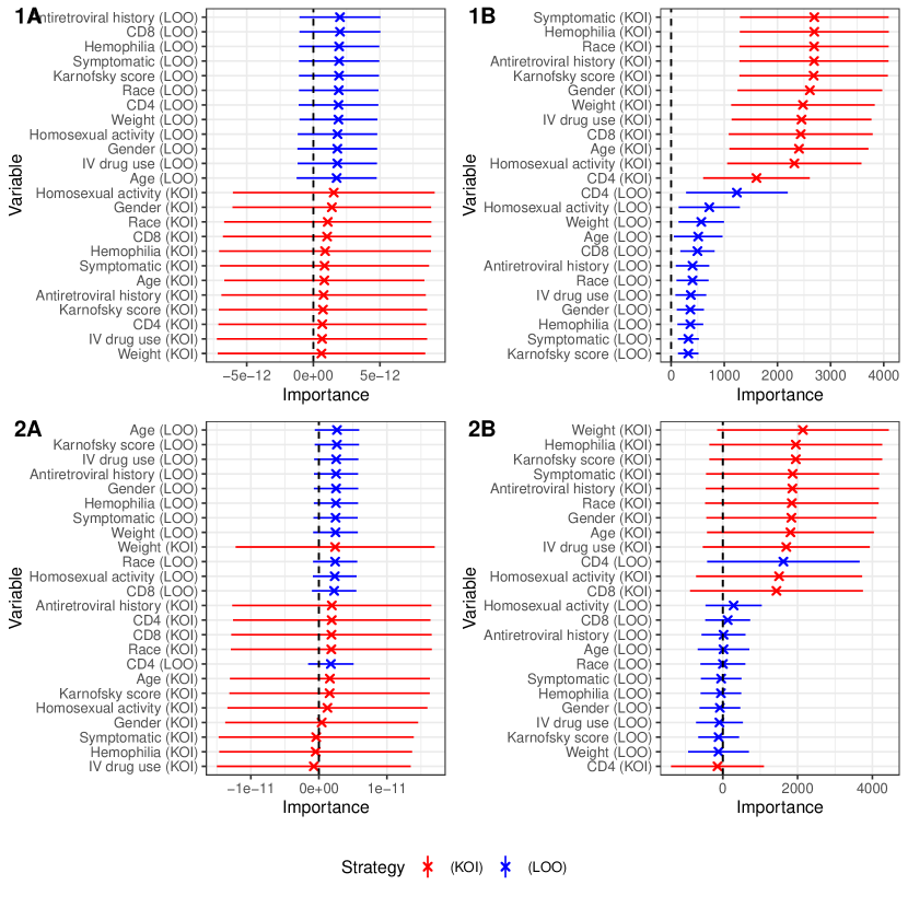
Figure 9: TE-VIM estimates $\hat{\Theta}_{s}$ from the ACTG175 study using modified Algorithms. Error bars indicate 95% CIs. In each plot, covariates are sorted according to their TE-VIM point estimate. Dashed lines indicate no importance. For the KOI mode, the TE-VIM represents the importance of the complement variable set, i.e. low-values denote high-importance of the KOI covariate.

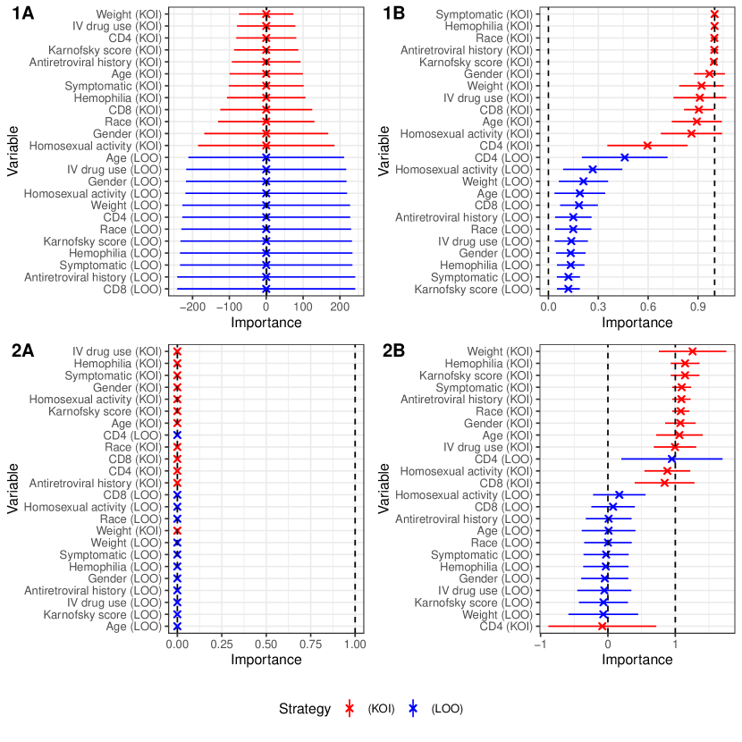
Figure 10: Scaled TE-VIM estimates $\hat{\Psi}_{s}$ from the ACTG175 study using modified Algorithms. Error bars indicate 95% CIs. In each plot, covariates are sorted according to their TE-VIM point estimate. Dashed lines indicate the $[0,1]$ support of the scaled TE-VIM. For the KOI mode, the TE-VIM represents the importance of the complement variable set, i.e. low-values denote high-importance of the KOI covariate.

References

- Abrevaya et al., (2015) Abrevaya, J., Hsu, Y. C., and Lieli, R. P. (2015). Estimating conditional average treatment effects. Journal of Business and Economic Statistics, 33(4):485–505.
- Athey and Imbens, (2016) Athey, S. and Imbens, G. (2016). Recursive partitioning for heterogeneous causal effects. Proceedings of the National Academy of Sciences of the United States of America, 113(27):7353–7360.
- Athey et al., (2019) Athey, S., Tibshirani, J., and Wager, S. (2019). Generalized random forests. Annals of Statistics, 47(2):1179–1203.
- Athey and Wager, (2021) Athey, S. and Wager, S. (2021). Policy learning with observational data. Econometrica, 89(1):133–161.
- Boileau et al., (2022) Boileau, P., Qi, N. T., van der Laan, M. J., Dudoit, S., and Leng, N. (2022). A flexible approach for predictive biomarker discovery. Biostatistics.
- Carone et al., (2018) Carone, M., Diaz, I., and van der Laan, M. J. (2018). Higher-order targeted loss-based estimation. In van der Laan, M. J. and Rose, S., editors, Targeted Learning in Data Science, Springer Series in Statistics, chapter 26. Springer International Publishing, Cham.
- Chen et al., (2020) Chen, H., Janizek, J. D., Lundberg, S., and Lee, S.-I. (2020). True to the model or true to the data? arXiv (2006.16234).
- Chernozhukov et al., (2018) Chernozhukov, V., Chetverikov, D., Demirer, M., Duflo, E., Hansen, C., Newey, W., and Robins, J. (2018). Double/debiased machine learning for treatment and structural parameters. Econometrics Journal, 21(1):C1–C68.
- Coston et al., (2020) Coston, A., Kennedy, E. H., and Chouldechova, A. (2020). Counterfactual predictions under runtime confounding. Advances in Neural Information Processing Systems, 2020-December(NeurIPS).
- Ding et al., (2016) Ding, P., Feller, A., and Miratrix, L. (2016). Randomization inference for treatment effect variation. Journal of the Royal Statistical Society. Series B: Statistical Methodology, 78(3):655–671.
- Grömping, (2009) Grömping, U. (2009). Variable importance assessment in regression: Linear regression versus random forest. The American Statistician, 63(4):308–319.
- Hammer et al., (1996) Hammer, S. M., Katzenstein, D. A., Hughes, M. D., Gundacker, H., Schooley, R. T., Haubrich, R. H., Henry, W. K., Lederman, M. M., Phair, J. P., Niu, M., Hirsch, M. S., and Merigan, T. C. (1996). A trial comparing nucleoside monotherapy with combination therapy in HIV-infected adults with CD4 cell counts from 200 to 500 per cubic millimeter. The New England Journal of Medicine, 335:1081–1090.
- Heckman et al., (1997) Heckman, J. J., Smith, J., and Clements, N. (1997). Making the most out of programme evaluations and social experiments : accounting for heterogeneity in programme impacts. Review of Economic Studies, 64(4):487–535.
- Hines et al., (2023) Hines, O., Diaz-Ordaz, K., and Vansteelandt, S. (2023). Optimally weighted average derivative effects. arXiv (2308.05456).
- Hines et al., (2022) Hines, O., Dukes, O., Diaz-Ordaz, K., and Vansteelandt, S. (2022). Demystifying statistical learning based on efficient influence functions. The American Statistician, 76(3):292–304.
- Hudson, (2023) Hudson, A. (2023). Nonparametric inference on non-negative dissimilarity measures at the boundary of the parameter space. arxiv (2306.07492).
- Huitfeldt et al., (2021) Huitfeldt, A., Fox, M. P., Murray, E. J., Hróbjartsson, A., and Daniel, R. M. (2021). Shall we count the living or the dead? New England Journal of Medicine, 259(25):1210–1214.
- Janzing et al., (2020) Janzing, D., Minorics, L., and Blöbaum, P. (2020). Feature relevance quantification in explainable ai: a causal problem. In International Conference on Artificial Intelligence and Statistics, pages 2907–2916. PMLR.
- Kallus, (2021) Kallus, N. (2021). More efficient policy learning via optimal retargeting. Journal of the American Statistical Association, 116(534):646–658.
- Kennedy, (2020) Kennedy, E. H. (2020). Optimal doubly robust estimation of heterogeneous causal effects. arXiv (2004.14497).
- Künzel et al., (2019) Künzel, S. R., Sekhon, J. S., Bickel, P. J., and Yu, B. (2019). Metalearners for estimating heterogeneous treatment effects using machine learning. Proceedings of the National Academy of Sciences of the United States of America, 116(10):4156–4165.
- Lei et al., (2018) Lei, J., G’Sell, M., Rinaldo, A., Tibshirani, R. J., and Wasserman, L. (2018). Distribution-free predictive inference for regression. Journal of the American Statistical Association, 113(523):1094–1111.
- Levy and van der Laan, (2018) Levy, J. and van der Laan, M. J. (2018). Kernel Smoothing of the Treatment Effect CDF. arXiv (1811.06514).
- Levy et al., (2021) Levy, J., van der Laan, M. J., Hubbard, A., and Pirracchio, R. (2021). A fundamental measure of treatment effect heterogeneity. Journal of Causal Inference, 9(1):83–108.
- Li et al., (2023) Li, H., Hubbard, A., and van der Laan, M. J. (2023). Targeted learning on variable importance measure for heterogeneous treatment effect. arXiv (2309.13324).
- Luedtke and van der Laan, (2016) Luedtke, A. R. and van der Laan, M. J. (2016). Super-learning of an optimal dynamic treatment rule. International Journal of Biostatistics, 12(1):305–332.
- Lundberg and Lee, (2017) Lundberg, S. M. and Lee, S.-I. (2017). A unified approach to interpreting model predictions. In Proceedings of the 31st international conference on neural information processing systems, pages 4768–4777.
- Murphy, (2003) Murphy, S. A. (2003). Optimal dynamic treatment regimes. Journal of the Royal Statistical Society: Series B (Statistical Methodology), 65(2):331–355.
- Newey and Robins, (2018) Newey, W. K. and Robins, J. M. (2018). Cross-fitting and fast remainder rates for semiparametric estimation. arXiv (1801.09138).
- Neyman, (1959) Neyman, J. (1959). Optimal asymptotic tests of composite statistical hypotheses. In Grenander, U., editor, Probability and Statistics: The Harald Cramer Volume, pages 213–234. Almqvist and Wiskell, Stockholm.
- Nie and Wager, (2021) Nie, X. and Wager, S. (2021). Quasi-oracle estimation of heterogeneous treatment effects. Biometrika, 108(2):299–319.
- Owen and Prieur, (2017) Owen, A. B. and Prieur, C. (2017). On Shapley value for measuring importance of dependent inputs. SIAM-ASA Journal on Uncertainty Quantification, 5(1):986–1002.
- Ribeiro et al., (2016) Ribeiro, M. T., Singh, S., and Guestrin, C. (2016). ”Why should I trust you?” explaining the predictions of any classifier. NAACL-HLT 2016 - 2016 Conference of the North American Chapter of the Association for Computational Linguistics: Human Language Technologies, Proceedings of the Demonstrations Session, pages 97–101.
- Robins et al., (1994) Robins, J. M., Rotnitzky, A., and Zhao, L. P. (1994). When some of regression coefficients estimation regressors are not always observed. Methods, 89(427):846–866.
- Rothwell, (2005) Rothwell, P. M. (2005). Subgroup analysis in randomised controlled trials: importance, indications, and interpretation. The Lancet, 365(9454):176–186.
- Rubin, (1974) Rubin, D. B. (1974). Estimating causal effects of treatments in randomized and nonrandomized studies. Journal of Educational Psychology, 66(5):688–701.
- Shannin and Brumback, (2022) Shannin, J. and Brumback, B. A. (2022). Death or survival, which you measure may affect conclusions: A methodological study. Health Science Reports, 5(6).
- Slamon et al., (2001) Slamon, D. J., Leyland-Jones, B., Shak, S., Fuchs, H., Paton, V., Bajamonde, A., Fleming, T., Eiermann, W., Wolter, J., Pegram, M., Baselga, J., and Norton, L. (2001). Use of chemotherapy plus a monoclonal antibody against HER2 for metastatic breast cancer that overexpresses HER2. New England Journal of Medicine, 344(11):783–792.
- Strobl et al., (2007) Strobl, C., Boulesteix, A.-L., Zeileis, A., and Hothorn, T. (2007). Bias in random forest variable importance measures: illustrations, sources and a solution. BMC Bioinformatics, 8(1):25.
- Syrgkanis et al., (2019) Syrgkanis, V., Lei, V., Oprescu, M., Hei, M., Battocchi, K., and Lewis, G. (2019). Machine learning estimation of heterogeneous treatment effects with instruments. Advances in Neural Information Processing Systems, 32.
- van der Laan, (2013) van der Laan, M. J. (2013). Targeted learning of an optimal dynamic treatment , and statistical inference for its mean outcome. UC Berkeley Division of Biostatistics Working Paper Series, (317):1–90.
- van der Laan and Gruber, (2016) van der Laan, M. J. and Gruber, S. (2016). One-step targeted minimum loss-based estimation based on universal least favorable one-dimensional submodels. International Journal of Biostatistics, 12(1):351–378.
- van der Laan and Luedtke, (2014) van der Laan, M. J. and Luedtke, A. R. (2014). Targeted Learning of the Mean Outcome under an Optimal Dynamic Treatment Rule. Journal of Causal Inference, 3(1):61–95.
- van der Laan et al., (2007) van der Laan, M. J., Polley, E. C., and Hubbard, A. E. (2007). Super learner. Statistical Applications in Genetics and Molecular Biology, 6(1).
- van der Vaart, (1998) van der Vaart, A. W. (1998). Empirical Processes. In Asymptotic Statistics, pages 265–290. Cambridge University Press.
- VanderWeele et al., (2019) VanderWeele, T. J., Luedtke, A. R., van der Laan, M. J., and Kessler, R. C. (2019). Selecting optimal subgroups for treatment using many covariates. Epidemiology (Cambridge, Mass.), 30(3):334.
- Verdinelli and Wasserman, (2021) Verdinelli, I. and Wasserman, L. (2021). Decorrelated variable importance. arXiv (2111.10853).
- Vermeulen and Vansteelandt, (2015) Vermeulen, K. and Vansteelandt, S. (2015). Bias-reduced doubly robust estimation. Journal of the American Statistical Association, 110(511):1024–1036.
- Wager and Athey, (2018) Wager, S. and Athey, S. (2018). Estimation and inference of heterogeneous treatment effects using random forests. Journal of the American Statistical Association, 113(523):1228–1242.
- Williamson and Feng, (2020) Williamson, B. D. and Feng, J. (2020). Efficient nonparametric statistical inference on population feature importance using Shapley values. 37th International Conference on Machine Learning, ICML 2020, PartF168147-14:10213–10222.
- (51) Williamson, B. D., Gilbert, P. B., Carone, M., and Simon, N. (2021a). Nonparametric variable importance assessment using machine learning techniques. Biometrics, 77(1):9–22.
- (52) Williamson, B. D., Gilbert, P. B., Simon, N. R., and Carone, M. (2021b). A general framework for inference on algorithm-agnostic variable importance. Journal of the American Statistical Association, 0(0):1–38.
- Wood et al., (2016) Wood, S. N., Pya, N., and Säfken, B. (2016). Smoothing parameter and model selection for general smooth models. Journal of the American Statistical Association, 111(516):1548–1563.
- Zaeri-Amirani et al., (2018) Zaeri-Amirani, M., Afghah, F., and Mousavi, S. (2018). A feature selection method based on Shapley value to false alarm reduction in ICUs a genetic-algorithm approach. Proceedings of the Annual International Conference of the IEEE Engineering in Medicine and Biology Society, EMBS, 2018-July:319–323.
- Zhang and Janson, (2020) Zhang, L. and Janson, L. (2020). Floodgate: inference for model-free variable importance. arXiv (2007.01283).
- Zhang et al., (2015) Zhang, Y., Laber, E. B., Tsiatis, A., and Davidian, M. (2015). Using decision lists to construct interpretable and parsimonious treatment regimes. Biometrics, 71(4):895–904.
- Zheng and van der Laan, (2011) Zheng, W. and van der Laan, M. J. (2011). Cross-validated targeted minimum-loss-based estimation. In Targeted Learning, pages 459–474. Springer New York, New York, NY.