A general study of decaying scalar dark matter: existing limits and projected radio signals at the SKA

Abstract

We consider a decaying scalar dark matter (DM) with mass $m_{\chi}$ in the range 10 GeV - 10 TeV and vary the branching ratios of all possible two-body SM final states (excluding and including $\nu\bar{\nu}$) in the range $0\%-100\%$ to derive constraints on the total decay width $\Gamma$ using the data collected by several astrophysical and cosmological observations. We find that, $\Gamma\lesssim 10^{-26}-10^{-27}\,{\rm s}^{-1}$ (excluding $\nu\bar{\nu}$) and $\Gamma\lesssim 10^{-24}-10^{-26}\,{\rm s}^{-1}$ (including $\nu\bar{\nu}$) are allowed, depending on the values of $m_{\chi}$, which are most robust upper limits on $\Gamma$ for a generic decaying scalar DM. We then investigate the prospect of the upcoming Square Kilometre Array (SKA) radio telescope in detecting the DM decay induced radio signals originating inside the dwarf spheroidal (dSph) galaxies. We have classified the DM parameter space, allowed by the existing observations, independently of the branching ratio of each individual two-body SM final state, based on the detectability at the SKA. Excluding the $\nu\bar{\nu}$ decay mode, we find that, throughout the DM mass range considered, $\Gamma\gtrsim 10^{-30}\,{\rm s}^{-1}-10^{-29}\,{\rm s}^{-1}$ is detectable for all possible branching ratio combinations at the SKA (assuming 100 hours of observation time), with conservative choices for the relevant astrophysical parameters. On the other hand, when arbitrary branching ratios are allowed also for the $\nu\bar{\nu}$ decay mode, DM decays can be probed independently of the branching ratio of each SM final state for $\Gamma\gtrsim 2\times 10^{-29}\,{\rm s}^{-1}$, provided DM masses are greater than a few hundreds of GeV.

1 Introduction

Various astrophysical and cosmological observations over the last few decades point towards the fact that an unavoidably large fraction of the total energy density of our Universe (about 23.4$\%$) is constituted by a yet unknown material component dubbed as ‘dark matter (DM)’ [1, 2, 3, 4]. A popular idea is that the DM consists of one or more unidentified massive elementary particle(s). An often discussed candidate is some Weakly Interacting Massive Particle (WIMP) [5, 6] whose mass lies in the GeV - TeV range. Mainly three experimental techniques, namely, direct search experiments, collider searches and indirect search observations, have been developed to detect such WIMP candidates. However, no confirmatory signals of the WIMP DM have been observed yet [7], and hence the need for the exploration of alternative scenarios of dark matter are largely felt. Among various proposed DM scenarios outside the WIMP paradigm, Feebly Interacting Massive Particles (FIMPs) [8], Strongly Interacting Massive Particles (SIMPs) [9], ELastically DEcoupling Relics (ELDERs) [10] etc., are the most popular ones. The common feature shared by most of these scenarios is the negligibly small interactions between the dark matter and the Standard Model (SM) particles. Various signals of such DM candidates have been studied extensively in the literature [11, 12, 13, 14, 15, 16, 17].

Such DM candidates, including WIMPs, are usually assumed to be absolutely stable. This immediately raises another curiosity: can the frequently postulated symmetry disallowing DM decays be broken in such a way that the DM candidate may decay into SM particle pairs at extremely slow rates? The observed large scale structure of our Universe requires the DM particle to be long-lived only on a cosmological time scale, and the possibility that the DM decays with a lifetime much larger than the age of the Universe is thus not inconceivable [18, 19, 20, 21, 22, 23, 24, 25, 26, 27, 28, 29, 30, 31, 32]. It is a likely proposition that the long-lived nature of the DM candidate is due to some continuous global symmetry [33, 34, 35]. Such a symmetry is liable to be broken at some level, albeit by a minuscule amount, thus causing extremely slow decays of the DM particle [28, 36, 37].

In such situations, if the only interactions of the DM candidate with the SM particles are those leading to DM decays, then the event rates in direct search or collider experiments are expected to be low. However, photons, antimatter particles and neutrinos, coming from the primary products of DM decays can still have substantial impacts on the data recorded in several cosmological and astrophysical observations. The mass of a decaying DM candidate is largely unconstrained [38, 30, 39, 40, 41]. Therefore, it is a common practice to phenomenologically restrict the space spanned by the DM mass and its decay width.

For example, Ref. [42] has put upper limits on the decay rate of a decaying scalar DM with mass in the keV - TeV range using the CMB anisotropy data collected by the Planck collaboration [4]. Specifically, the energy injections by the stable SM decay products of the DM candidate, into the photon-baryon plasma during the cosmic dark ages perturb the CMB anisotropy spectra, which is severely constrained by the Planck data [4]. The isotropic gamma-ray background (IGRB), on the other hand, may receive contributions from the gamma-ray fluxes produced in the DM decays, in addition to the dominant contributions coming from the active galactic nuclei (AGN) and the star-forming galaxies. Thus the IGRB fluxes measured by SAS-2 [43], EGRET [44], Fermi-LAT [45, 46] etc., can be compared against the gamma-ray fluxes induced by a decaying DM candidate to derive upper bounds on the DM decay width for the chosen value of the DM mass [47, 48].

In the matter sector, antimatter particles are likely to form even more spectacular DM signals. Thus, the data from the antimatter searches performed by CAPRICE [49], HEAT [50], AMS-01 [51], PAMELA [52], AMS-02 [53, 54, 55] etc., can be used to set upper limits on the DM decay generated antimatter fluxes which in turn give stringent constraints on the parameter space of a decaying DM particle [56, 57, 58]. In addition, neutrino fluxes induced by the DM decay products are also detectable in several neutrino telescopes and hence, neutrino observations by Super-Kamiokande [59, 60], IceCube [60, 61, 62, 63] etc., too, contribute to the existing limits on decaying DM. Multi-messenger analyses using the data taken by several gamma-ray, cosmic-ray and neutrino observations, are also available in the literature [64].

Yet another signature of decaying DM consists in the radio synchrotron emission from the $e^{+}e^{-}$ pairs originating in DM decays occurring inside DM dominated galaxies and clusters. These electrons (positrons) undergo energy loss via electromagnetic interactions in the interstellar medium and give rise to radio waves. Nearby dwarf spheroidal (dSph) galaxies are popular sources for studying such radio signals, because of their low-star formation rates and high mass-to-light ratios [65, 66, 67, 68] which ensure a comparatively lower astrophysical background and larger DM abundance inside them.

Data taken by several existing radio observations have been used to draw constraints on the DM parameter space [69, 70, 71, 72, 73, 74, 75]. The prospect of the upcoming Square Kilometre Array (SKA) radio telescope is found to be quite encouraging in this regard [76, 77, 78, 79, 80, 81]. In fact, Ref. [81] has shown that the SKA can probe much deeper into the parameter space of a decaying DM compared to the existing gamma-ray observations. The inter-continental baseline lengths of the SKA allow one to efficiently resolve the astrophysical foregrounds and its large effective area helps to achieve higher surface brightness sensitivity [82] compared to other existing radio telescopes. In addition, large frequency range of the SKA, i.e., 50 MHz - 50 GHz, has important implications for DM masses in the GeV - TeV range.

A common practice in the existing studies of decaying DM is to assume that the DM decays into a specific two-body SM final state at a time with 100$\%$ branching ratio and then the DM parameter space is constrained by using the data of various cosmological and astrophysical observations [42, 83, 47, 48, 56, 57, 64]. Any specific assumption about the branching fraction of each individual DM decay mode is equivalent to committing to a particular underlying DM model. However, in a generic model the DM candidate may decay to any arbitrary final state with a priori undetermined branching ratios. Thus the limits obtained in such cases, are quite different from the limits derived assuming 100$\%$ branching ratio for any SM final state.

We have taken an unbiased approach and allowed the branching fractions of all kinematically allowed two-body SM final states of the decaying scalar DM ($\chi$), to take arbitrary values in the range $0\%-100\%$, while deriving the constraints on the total DM decay width ($\Gamma$), for the DM mass ($m_{\chi}$) in the range 10 GeV - 10 TeV. We have additionally assumed that $\chi$ saturates the entire relic density of the Universe. A similar study for the annihilating WIMP DM can be found in [84]. It was found there that, the allowed region of the DM parameter space is substantially enlarged when the above-mentioned approach is adopted.

In deriving the upper limit on total $\Gamma$, i.e., $\Gamma_{\rm max}$, we have used the data from the Planck CMB [4], Fermi-LAT isotropic gamma-ray background (IGRB) [46] and AMS-02 positron flux [53] observations. We have also utilized the observational data of the Super-Kamiokande neutrino flux measurement [59] while including DM decays to SM neutrinos (i.e., $\chi\rightarrow\nu\bar{\nu}$) in our analysis.

We emphasize that, the $\nu\bar{\nu}$ decay mode can be constrained not only by the neutrino observations such as Super-Kamiokande [59], but also by the data of Planck CMB [4], Fermi-LAT IGRB [46] and AMS-02 positron flux [53] observations. This is because, the final state $\nu\bar{\nu}$ pairs give rise to $e^{+}(e^{-})$ and $\gamma$-ray photons via the radiation of electroweak gauge bosons. This process is suppressed by the $SU(2)_{L}$ gauge coupling and the gauge boson masses. As a result, the rates of $e^{+}(e^{-})$ and $\gamma$ production are thus sizeable only when the (anti)neutrinos are energetic enough to produce on-shell $W$ and $Z$-bosons. Note that the $\nu\bar{\nu}$ final state was not considered in deriving the constraints on the total cross-section of annihilating WIMPs [84]. However, it should also be emphasized that the constraints on this final state coming from the data collected by the neutrino telescopes [85, 59, 60, 62, 63] may be stronger than those obtained from the data of other astrophysical observations [42].

We have studied several scenarios differing from each other in the branching ratio attributed to the $\nu\bar{\nu}$ decay mode. In each case, the obtained value of $\Gamma_{\rm max}$ is independent of the specific branching ratios of individual SM final states and there exists no possible branching ratio combinations for which any value of $\Gamma$ greater than $\Gamma_{\rm max}$ is allowed by the existing data. It is found that, $\Gamma_{\rm max}$ obtained here can be considerably weaker compared to the limits obtained when 100$\%$ branching ratio is assumed for each individual DM decay mode.

In the next step, parts of the DM parameter space allowed by the existing astrophysical and cosmological observations are classified based on the detectability at the SKA assuming 100 hours of observation towards the Segue 1 (Seg 1) dSph. In each scenario, for every given $m_{\chi}$, we found the maximum and the minimum radio flux distributions by varying the branching ratios of all two-body SM final states in the range $0\%-100\%$. The radio fluxes predicted for all branching ratio combinations lie between these maximum and minimum fluxes in every frequency bin. The SKA detectability is then determined depending on whether these maximum and minimum fluxes are above or below the SKA sensitivity level obtained assuming 100 hours of observation time.

The detectability at the SKA is presented by dividing the allowed portions of the $m_{\chi}-\Gamma$ plane into three separate regions marked as green, yellow and red. The green regions consist of those parameter points which are detectable for all possible branching ratio combinations of the kinematically allowed two-body SM final states of the DM while the yellow regions cover the parts of the DM parameter space that are only detectable for certain specific branching ratio combinations. Regions of the $m_{\chi}-\Gamma$ plane which are not detectable at the SKA (in the 100 hours of observation) for any possible branching ratio combinations, are marked red. Note that with more hours of observation time some parts of these non-detectable regions of the DM parameter space will also become accessible. We have also indicated how the variations of the astrophysical parameters affect our capability to probe the decaying DM parameter space. Our study shows that, the SKA will explore a much wider region of the decaying DM parameter space compared to the existing observations, not only when DM decays to visible SM final states are considered but also when $\chi\rightarrow\nu\bar{\nu}$ channel is included in the analysis.

Our study is ‘model-independent’ in the sense that we have not adhered to any definite theoretical framework or specific terms in the DM Lagrangian, which determine the branching ratio of each individual decay mode. The following assumptions are in built in the study, largely for simplicity:

• The scalar $\chi$ decays only into two-body SM final states.

• $\chi$ decays into fermion pairs are flavour diagonal and also lepton-number conserving.

• The hadronic showers of $\chi$ decays are faithfully simulated using $\mathtt{Pythia}$ [86].

The paper is organized as follows: in Sec. 2 we discuss a few salient features of our study followed by presenting the limits on individual DM decay modes coming from the Planck CMB, Fermi-LAT IGRB, AMS-02 positron flux and Super-Kamiokande neutrino flux observations. In Sec. 3 we derive the upper limit on the total DM decay width using the data of the above-mentioned observations. A brief review of the generation of the radio synchrotron signals from the DM decays within the dwarf galaxies is given in Sec. 4.1, while in Sec. 4.2 we outline the methodology we have adopted to classify the allowed part of the DM parameter space based on the detectability at the SKA. In Sec. 5 we present the projected reach of the SKA. Finally, we summarize and conclude in Sec. 6.

2 Decaying dark matter: a status review

As mentioned in the introduction, here we study the implications of the two-body decays of a scalar DM in the context of indirect search observations. In this section, we first give a brief review of some existing decaying DM scenarios with DM mass in the GeV - TeV range and thereby motivate the assumptions we have made in our study. Thereafter, we present the limits on $\Gamma$ as a function of $m_{\chi}$ obtained using the data coming from different existing astrophysical and cosmological observations assuming DM decays to a single channel at a time. This sets the stage for our subsequent analysis.

2.1 Motivations and theoretical approach

In most scenarios beyond the Standard Model (BSM), the DM candidate is stabilized by imposing an ad-hoc symmetry which is somewhat inexplicable other than in a few well-motivated scenarios like the R-parity conserved Minimal Supersymmetric Standard Model (MSSM). Moreover, continuous global symmetries may be broken by interactions suppressed by the Planck scale [36, 37, 28]. Therefore, scenarios where the GeV - TeV scale DM particles are stable in the cosmological time scales but decay afterwards, are not uncommon [18, 19, 20, 21, 22, 23, 24, 25, 26, 27, 28, 29, 30, 31, 32].

For example, in R-parity violating supersymmetric (SUSY) scenarios, gravitinos ($\tilde{G}$) [18, 19, 20] and axinos ($\tilde{a}$) [21, 22] are two possible decaying DM candidates. Decaying gravitino lightest superparticles (LSPs) of $\mathcal{O}({\rm GeV})$ masses can serve as viable candidates for DM in several extensions of R-parity violating SUSY scenarios [18, 19] with observable signatures in various gamma-ray observations [20]. In addition, GeV scale axinos are also potential candidates for the decaying DM [21] providing explanations for the Fermi-LAT 130 GeV gamma-ray excess [22]. This excess [87, 88] can also be explained by the scalar partner $\tilde{\phi}$ of a chiral superfield $\Phi$ which serves as the DM and decays to $\gamma\gamma$ or $\gamma\,Z$ final states via global $U(1)_{R}$ breaking interactions [26].

Several scenarios of TeV-scale decaying scalar DM which decays to SM leptons [89, 90, 24, 25, 30] have been proposed in the context of the positron excesses observed in PAMELA [52] and AMS-02 [91]. Apart from these, decays of GeV - TeV scale scalar DM particles via non-minimal couplings to the Ricci scalar (R) [31] or via higgs-gravity portal interactions [32] are also studied in the literature. In the SUSY context, right-handed sneutrinos ($\tilde{\nu}_{R}$) couple to left-handed sneutrinos ($\tilde{\nu}_{L}$) via Dirac neutrino Yukawa coupling and decays to SM leptons by means of the trilinear R-parity breaking interaction terms [29]. When R-parity is conserved the heavier $\tilde{\nu}_{R}$ decays to the lighter $\tilde{\nu}_{R}$ and gives rise to a photon spectrum with sharp-spectral feature [23].

As mentioned earlier, here we have varied the decaying DM mass in the range 10 GeV - 10 TeV but refrain from assuming any specific mechanism for DM production. Most of the existing indirect search observations including the ones we have considered here (i.e., Planck CMB [4], Fermi-LAT IGRB [46], AMS-02 positron flux [53] and Super-Kamiokande neutrino flux [59] measurements), are sensitive to the signals of WIMP annihilations. The spectra of photons, antimatter particles and neutrinos, originating from scalar DM particles decaying into two-body SM final states are similar to that coming from the WIMP annihilations and thus most stringent constraints from such observations can be derived for decaying DM particles in the GeV - TeV mass range [92]. Additionally, the next generation observations such as the upcoming SKA radio telescope is also sensitive to the signals of DM particles in the GeV - TeV mass range [81, 78]. Therefore, our choice of the DM mass range is primarily motivated by phenomenological considerations and potential for detections rather than theoretical arguments.

For heavier DM particles there exist a number of gamma-ray, cosmic-ray and neutrino observations which provide quite strong constraints [64]. The upcoming Cherenkov Telescope Array (CTA) will also be quite useful in constraining DM particles heavier than a few tens of TeV [93, 94, 95]. On the other hand, in case of keV and MeV DM particles X-ray [96] and CMB [42] constraints are the most stringent ones, till date. In addition, gamma-ray searches by ACT [97], GRIPS [98], AdEPT [99], COMPTEL [100], EGRET [101] etc. and positron observation of Voyager I [102, 103] have been used to constrain the parameter space of a MeV-scale decaying DM [104, 105]. Apart from these, future MeV $\gamma$-ray experiments like e-ASTROGRAM [106], AMEGO [107], GRAMS [108] etc. will also have important implications for decaying DMs with masses in the MeV range. However, for such DM particles, detection at the SKA depends on other mechanism such as the inverse compton (IC) effect. The frequency distribution in such a case is different from what is predicted by simulating synchrotron emission in the dSph galaxies [79]. This is kept beyond the scope of the present work.

Any specific theoretical scenario would clearly identify some preferred DM decay modes with known branching fractions, provided we know the Lagrangian for the concerned model (see, for example, [81]). However, without being governed by any such model, here, we consider a scalar DM in the mass range 10 GeV - 10 TeV, which accounts for the entire dark matter energy density of the Universe, and decays into all possible two-body SM final states, i.e., $\chi\rightarrow$ ${\rm SM}_{1}$ $\mkern 1.5mu\overline{\mkern-1.5mu\rm SM\mkern-1.5mu}\mkern 1.5mu_{2}$, where ${\rm SM}_{1}$ $\mkern 1.5mu\overline{\mkern-1.5mu\rm SM\mkern-1.5mu}\mkern 1.5mu_{2}$ belongs to the following set: $\{e^{+}e^{-}$, $\mu^{+}\mu^{-}$, $\tau^{+}\tau^{-}$, $b\bar{b}$, $t\bar{t}$, $q\bar{q}$, $W^{+}W^{-}$, $ZZ$, $\gamma\gamma$, $gg$, $hh$, $Z\gamma$, $Zh$, $\nu\bar{\nu}\}$. Note that, as mentioned in the introduction, unlike most of the studies available in the literature, we have also considered DM decays to $\nu\bar{\nu}$, in our analysis.

We would like to point out that in case of the $\nu\bar{\nu}$ final state $\nu_{e},\nu_{\mu}$ and $\nu_{\tau}$ flavours are assumed to be produced with equal branching fractions, the sum of which determines the total branching ratio of the $\nu\bar{\nu}$ channel. Similarly, while considering the $q\bar{q}$ decay mode we have assumed that $u\bar{u},d\bar{d},c\bar{c}$ and $s\bar{s}$ final states are produced with equal branching ratios so that their sum equals the total branching fraction attributed to the $q\bar{q}$ final state. For any given value of $m_{\chi}$ only the kinematically allowed two-body SM final states are taken into account. For example, if $m_{\chi}{\;\raise 1.29167pt\hbox{$<$\kern-7.5pt\raise-4.73611pt\hbox{$\sim$}}\;}160\,{\rm GeV}$, branching ratio for the $W^{+}W^{-}$ final state has been set to zero throughout the analysis.

Furthermore, in our study we have implicitly assumed that there exists no BSM decay mode of the DM candidate such as the dark radiation. As we had mentioned earlier, we have also ignored any possible flavour violating decays (e.g., $\chi\rightarrow\mu\tau,d\bar{s}$) and lepton number violating decays (e.g., $\chi\rightarrow\nu\nu,\bar{\nu}\bar{\nu}$). These assumptions are usually valid in minimal models of decaying DM. However, inclusions of such decay modes would not change the results presented here substantially.

In the line of several existing works on decaying DM (see, for example [92, 48, 81] etc.), we have based our analysis on the postulate that all indirect signals in the form of $\gamma$-rays, electrons (positrons), $\nu\bar{\nu}$ and radio waves arise from DM decays only, and the contributions of DM annihilations to such signals are negligible. Thus, using the data from different indirect search observations, the maximum amount of flux arising from DM decay can be constrained for any $m_{\chi}$. These maximum values are realized in situations where DM annihilations into SM particle pairs have negligible rates. In these cases, the DM is then either produced non-thermally in the decay of superheavy states [27], or freezes out via the participation of some hidden sector particles [39, 109]. The observed relic density of our Universe is generated in this manner. On the other hand, DM decays to SM particle pairs can take place via several hitherto unknown effective interactions which are not necessarily correlated with the production mechanism of the DM candidate. Such effective interactions driving the DM decays are usually obtained on integrating out various heavy fields and thus the resulting decay processes are slow enough to evade the existing constraints from the indirect search observations.

2.2 Indirect detection signals and existing constraints

Indirect detection of GeV - TeV scale decaying DM consists in detecting the gamma-ray photons, electrons-positrons (along with various electromagnetic signals originating from them) and neutrino-antineutrino pairs coming from the cascade decays of the SM particles which are produced as the primary decay products of the DM. Usually the data from several observations are used to constrain the DM parameter space assuming 100$\%$ branching ratio for each individual SM final state. However, our goal here is to obtain an upper limit on the total $\Gamma$ independent of the branching fraction of each individual DM decay modes. For this purpose, it is necessary to calibrate our analysis technique first.

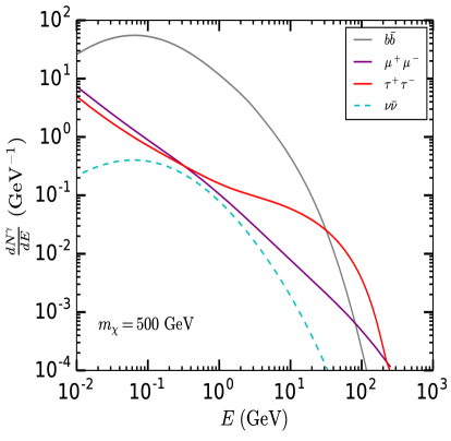
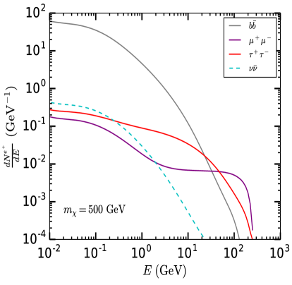
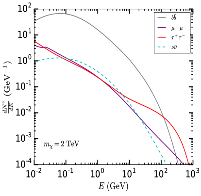
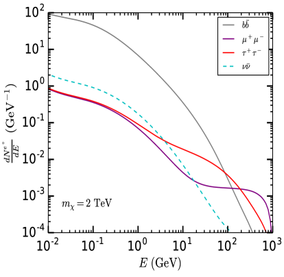
Figure 1: Top: The photon spectra $dN^{\gamma}/dE$ (left panel) and positron spectra $dN^{e^{+}}/dE$ (right panel) are shown for $b\bar{b}$ (gray solid line), $\mu^{+}\mu^{-}$ (purple solid line), $\tau^{+}\tau^{-}$ (red solid line) and $\nu\bar{\nu}$ (cyan dashed line) final states assuming $100\%$ branching ratio for each individual channels for a benchmark value of $m_{\chi}=500\,{\rm GeV}$. Bottom: The corresponding distributions for $m_{\chi}=2\,{\rm TeV}$ are shown. See the text for details.

Note that, unlike most of the studies found in the literature, we have included the effect of the $\nu\bar{\nu}$ final state. As mentioned in the introduction, for this final state, the photons and electrons (positrons) are produced by the radiation of electroweak gauge bosons and hence, the resulting spectra are highly suppressed for $m_{\chi}$ lower than a few hundreds of GeV. This is because, for such values of $m_{\chi}$ the final state $\nu\bar{\nu}$ pairs are of low energy. However, for heavier DM particles, the $\nu\bar{\nu}$ pairs are highly energetic, so that the on-shell $W$ and $Z$ bosons are abundantly radiated from them. Consequently, the produced $\gamma$ and $e^{+}(e^{-})$ spectra are comparable to the corresponding spectra coming from other SM final states.

In the top left panel of Fig. 1, considering $m_{\chi}=500\,{\rm GeV}$, we have shown the $\gamma$-ray spectra $dN^{\gamma}/dE$ produced per DM decay, for the $b\bar{b}$ (gray solid line), $\mu^{+}\mu^{-}$ (purple solid line), $\tau^{+}\tau^{-}$ (red solid line) and $\nu\bar{\nu}$ (cyan dashed line) final states assuming $100\%$ branching ratio for each individual channel. In the top right panel, the $e^{+}$ spectra $dN^{e^{+}}/dE$ (same as the $e^{-}$ spectra $dN^{e^{-}}/dE$) for these DM decay modes are shown. It is evident that, the spectra coming from the $\nu\bar{\nu}$ final state are considerably suppressed compared to those from the $b\bar{b}$ final state throughout the energy range. In the higher energy bins, the fluxes originating from the $\nu\bar{\nu}$ channel are suppressed compared to the spectra of the $\mu^{+}\mu^{-}$ and $\tau^{+}\tau^{-}$ channels, too. As one decreases $m_{\chi}$, the spectra corresponding to the $\nu\bar{\nu}$ final state become even more subdominant. On the other hand, on increasing $m_{\chi}$, photon and positron (electron) fluxes coming from the $\nu\bar{\nu}$ decay mode are enhanced throughout the energy range, as shown in the bottom panels of Fig. 1, where $m_{\chi}=2\,{\rm TeV}$ is assumed. The photon and positron (electron) spectra presented here are obtained from the $\mathtt{Pythia}$ [86] generated files provided by the $\mathtt{PPPC4DMID}$ [110, 111, 112] and will be used in the upcoming analyses.

Keeping this in mind, in this section we go ahead to present the constraints on the DM parameter space for each individual observation, i.e., Planck CMB [4], Fermi-LAT IGRB [46], AMS-02 cosmic-ray positron flux [53] and Super-Kamiokande neutrino flux [59] measurements, assuming the DM decays to any given two-body SM final state with 100$\%$ branching ratio. This will enable us to include the effect of arbitrary branching fractions to all channels in our analysis.

2.2.1 Planck CMB constraints

Energy injections to the photon-baryon fluid between recombination ($z\sim 1100$) and reionization ($z\sim 6$) can alter the thermal history of the Universe and thereby causes perturbations to the CMB anisotropy spectra. In scenarios with unstable DM candidates, the SM particles produced in the DM decays act as additional sources of energy injections during the cosmic dark ages to distort the CMB anisotropy spectra. On the other hand, the CMB is quite accurately measured by the Planck collaboration [4] and any substantial distortion in the CMB spectrum is ruled out by the Planck data [4]. Therefore, the data of the CMB observation by Planck [4] can be employed to constrain the fluxes of $\gamma$, $e^{-}$ and $e^{+}$ coming from the DM decays. This in turn implies upper limits on $\Gamma$ for any $m_{\chi}$, since these fluxes of stable SM particles are proportional to the DM decay width for any given value of the DM mass.

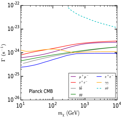
Figure 2: 95% C.L. upper limits on $\Gamma$ assuming 100% branching ratio for each SM final state, are obtained from the Planck observation of the temperature and polarization anisotropies of CMB. Here, we show the constraints for seven SM final states for the purpose of illustration.

Here, we shall follow the methodology outlined in Ref. [42] to derive the Planck CMB [4] constraints on $\Gamma$ for $m_{\chi}$ in the range 10 GeV - 10 TeV. Ref. [42] has used the technique of principal component analysis (PCA) to derive constraints on a generic decaying scalar DM. The 95$\%$ confidence level (C.L.) upper limit on $\Gamma$ is given by [42]:

$$\Gamma\lesssim\left(\frac{\vec{N}.\vec{e}_{1}}{\vec{e}_{1}(30\,{\rm MeV}\,e^{+}e^{-})}\right)^{-1}\,\left(2.6\times 10^{25}\,{\rm s}\right)^{-1},$$ (2.1)

where $\vec{e}_{1}$ is the first principal component (PC) and $\vec{N}$ contains the information of the $e^{+}$ ($e^{-}$) or the $\gamma$ spectra for the considered DM decay mode:

$$\vec{N}=\left\{\sum_{f}\,B_{f}\frac{1}{m_{\chi}}E_{i}\frac{dN_{f}^{e^{+}}}{d\ln E_{i}}(E_{i}),\sum_{f}\,B_{f}\frac{1}{m_{\chi}}E_{i}\frac{1}{2}\frac{dN_{f}^{\gamma}}{d\ln E_{i}}(E_{i})\right\},$$ (2.2)

with $i=1,2,...,N$ signifying the respective energy bins spanning the entire considered energy range 10 keV - 1 TeV [42], $f$ being the two-body SM final state with branching ratio $B_{f}$, while, as mentioned earlier, $dN_{f}^{e^{+}}/d\ln E$ ($dN_{f}^{e^{-}}/d\ln E$) and $dN_{f}^{\gamma}/d\ln E$, respectively, represent the $e^{+}(e^{-})$ and $\gamma$ spectra associated with per DM decay to the final state $f$.

The first principal component $\vec{e}_{1}$ is the eigenvector corresponding to the largest eigenvalue of the marginalized Fisher matrix. The Fisher matrix is constructed out of the perturbations to the CMB anisotropy spectra caused by the basis energy injection models (see Ref. [42] for details). In Eqn. 2.1, $\vec{e}_{1}(30\,{\rm MeV}\,e^{+}e^{-})$ represents the value of the first PC for the $e^{+}e^{-}$ final state with an injection energy of 30 MeV which is chosen as a reference model in Ref. [42]. $\vec{N}.\vec{e}_{1}$ represents the projection of $\vec{N}$ on the first PC. For calculating $\vec{N}.\vec{e}_{1}$, in Eqn. 2.1, the contributions of both $\gamma$ and $e^{+}(e^{-})$ are taken into account. The first PC $\vec{e}_{1}$ for both $\gamma$ and $e^{+}(e^{-})$ (for injection energies 10 keV - 1 TeV) are taken from [42] to which the readers are referred for the details of the analysis methodology.

Using Eqn. 2.1, we have derived the CMB constraints on the $m_{\chi}-\Gamma$ plane assuming DM decays to a specific SM final state with 100$\%$ branching ratio. We have shown our results for seven illustrative DM decay modes in Fig. 2. As mentioned earlier, the spectra of $e^{+}(e^{-})$ and $\gamma$ coming from $\chi\rightarrow\nu\bar{\nu}$ decay mode are comparable to that originating from other SM final states only when $m_{\chi}$ is larger than a few hundreds of GeV (see Fig. 1). As a result, the constraint on the $\nu\bar{\nu}$ channel also strengthens in this $m_{\chi}$ range (see cyan line in Fig. 2).

2.2.2 Fermi-LAT IGRB constraints

Gamma-ray photons are produced as one of the end products of the decay cascades of the SM particles originated in the decays of GeV - TeV scale DM particles. In case of the hadronic decay modes, $\pi^{0}\rightarrow\gamma\gamma$ acts as the source of such gamma-ray photons, while for the leptonic decay channels, these photons are dominantly produced from the final state radiations. Direct decay of DM to $\gamma\gamma$ is also possible. In addition, $e^{+}e^{-}$ produced from the DM decays also upscatter photons of the interstellar radiation field (ISRF) to gamma-ray energies and contribute to the gamma-ray signals of decaying DM.

For any given value of $m_{\chi}$, the gamma-ray flux is proportional to the DM decay width and larger the value of $\Gamma$ greater is the expected signal. Thus, the gamma-ray flux measured by any observation can be compared against the fluxes predicted from the decay of a DM particle of mass $m_{\chi}$ in any suitably chosen astrophysical source and the corresponding upper limit on $\Gamma$ can be derived. In case of a decaying DM scenario the gamma-ray flux from an extra-terrestrial source is proportional to a single power of the DM density in that source and broader the source is larger is the expected gamma-ray signal. Thus, for a decaying DM scenario most stringent upper limits from the gamma-ray observations are usually obtained when one considers the isotropic component of the signal, i.e., the extra-galactic component [113, 92]. As a result, in the case of a decaying dark matter Fermi-LAT IGRB constraints are more stringent than those coming from the Fermi-LAT observations of other gamma-ray sources such as the dSph galaxies [114].

The extra-galactic gamma-ray flux from the DM decays is given by [47, 83, 110],

$$\frac{d\Phi^{\rm EG}}{dE_{\gamma}} = \frac{\Gamma}{4\pi m_{\chi}}\,c\,\Omega_{\rm DM}\,\rho_{c}\sum_{f}B_{f}\int_{0}^{\infty}\,dz\frac{1}{H(z)}e^{-\tau(E_{\gamma},z)}\bigg{[}\frac{dN^{\gamma}_{f}}{dE_{\gamma}}(E_{\gamma}(1+z))$$

$$+\frac{2}{E_{\gamma}(1+z)}\int_{m_{e}}^{m_{\chi}/2}dE_{e}\frac{P^{\rm CMB}_{\rm IC}(E_{\gamma},E_{e},z)}{b^{\rm CMB}_{\rm IC}(E_{e})}\int_{E_{e}}^{m_{\chi}/2}d\tilde{E}_{e}\frac{dN^{e^{+}}_{f}}{d\tilde{E}_{e}}(\tilde{E}_{e})\bigg{]},$$

where DM density $\Omega_{\rm DM}$, critical density $\rho_{c}$ and all other relevant parameters needed to evaluate the redshift dependent Hubble parameter $H(z)$ are taken from Ref. [4]. For the optical depth $e^{-\tau(E_{\gamma},z)}$, the inverse compton scattering (ICS) power $P^{\rm CMB}_{\rm IC}$ and the energy loss term $b^{\rm CMB}_{\rm IC}$ we have used the parameterizations given in [110, 115].

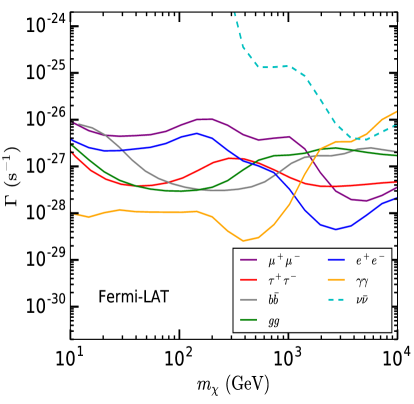
Figure 3: 95% C.L. upper limits on $\Gamma$ (for seven illustrative decay modes) derived from the data of the Fermi-LAT IGRB observation are shown. In deriving these limits 100% branching ratio is attributed to each individual DM decay channel.

The diffuse isotropic gamma-ray background (IGRB) in the energy range 100 MeV - 820 GeV [46] is measured by the Fermi Large Area Telescope (Fermi-LAT) during its 50 months of observation time and provides the most stringent $\gamma$-ray constraints on the parameter space of a GeV - TeV scale decaying DM [29, 47, 48]. In deriving these constraints we have followed the methodology of [47] and parameterized the background gamma-ray flux as [46],

$$\frac{d\Phi^{\rm BG}}{dE_{\gamma}}=I_{100}\left(\frac{E_{\gamma}}{100\,{\rm MeV}}\right)^{-\beta}\,\exp\left(-\frac{E_{\gamma}}{E_{c}}\right).$$ (2.4)

Then we perform a likelihood ratio test with the $\chi^{2}$ defined as:

$$\chi^{2}=\sum_{i}\,\frac{\left(\Phi^{\rm BG}(E_{i})+\Phi^{\rm EG}(E_{i})-D_{i}\right)^{2}}{\sigma^{2}_{i}},$$ (2.5)

where $D_{i}$ is the Fermi-LAT IGRB data [46], $\Phi^{\rm BG}(E_{i})$ is the expected number of background events and $\Phi^{\rm EG}(E_{i})$ is the expected number of signal events in the $i$-th energy bin while $\sigma_{i}$ is the associated uncertainty [46]. We then minimize the $\chi^{2}$ in Eqn. 2.5 with respect to the parameters $\{I_{100},\beta,E_{c},\Gamma\}$ to obtain the best-fit values of these parameters which give us the best-fit value of $\chi^{2}$, i.e., $\chi^{2}_{\rm bf}$. Then all other parameters are kept fixed at their best-fit values while $\Gamma$ is increased until the $\chi^{2}$ increases by 2.71 from its best-fit value, i.e.,

$$\chi^{2}(\Gamma)=\chi^{2}_{\rm bf}+2.71,$$ (2.6)

which gives us the $95\%$ C.L. upper limit on $\Gamma$. For details of the analysis methodology adopted here we refer the reader to Ref. [47].

Assuming the DM decays to a specific SM final state with $100\%$ branching ratio the $95\%$ C.L. upper limits on $\Gamma$ obtained using Eqn. 2.6 are shown in Fig. 3, for seven different DM decay modes. As one can see from Fig. 3, for $m_{\chi}{\;\raise 1.29167pt\hbox{$<$\kern-7.5pt\raise-4.73611pt\hbox{$\sim$}}\;}1\,{\rm TeV}$, the limit on the $\gamma\gamma$ final state is most stringent while the limit is weakest for $\mu^{+}\mu^{-}$. For $m_{\chi}$ greater than $\sim 1\,{\rm TeV}$ the constraint weakens considerably for $\gamma\gamma$ channel, since, the energies of the produced photons fall outside the sensitivity range of Fermi-LAT. One interesting point to note that the constraint on the $\nu\bar{\nu}$ channel becomes stronger than that for the $\gamma\gamma$ channel in the DM mass range $3\,{\rm TeV}$ - $10\,{\rm TeV}$ (cyan line in Fig. 3). This is because, as mentioned previously, for the $\nu\bar{\nu}$ channel the $\gamma$-rays come from the electroweak gauge bosons which are abundantly radiated only when the DM mass is on the higher side (see Fig. 1).

2.2.3 AMS-02 positron constraints

Among the stable SM particles produced as the final products of DM decay cascades positrons are another powerful probes for understanding the nature of DM interactions. The SM particles produced from the DM decays give rise to electrons-positrons via cascade decays and the produced positrons undergo diffusion and energy losses in the galactic medium before reaching the detectors devised to detect cosmic-ray positrons. The positron spectra coming from DM decays are governed by $\Gamma$ for any given $m_{\chi}$ and for specific choices of the astrophysical parameters governing the DM density distribution and positron propagation inside the Milky Way (MW) galaxy. Therefore, stringent upper limits on $\Gamma$ are derived by comparing the DM decay induced positron flux against the measured value of the cosmic-ray positron flux when all other parameters are kept fixed. The measurement of the cosmic-ray positron flux [53] by the Alpha Magnetic Spectrometer (AMS) on the International Space Station (ISS) provides strong constraints on the parameter space of a decaying dark matter [56, 57].

The propagation of the positrons produced from DM decays is governed by the diffusion-loss equation. After ignoring the convection and the diffusion terms in the momentum space which do not affect the positron spectra for the energy range of interest [116], this equation is given by [84]:

$$\frac{\partial N_{i}}{\partial t}=\vec{\nabla}.(D\vec{\nabla})N_{i}+\frac{\partial}{\partial p}(b(p,\vec{r}))N_{i}+Q_{i}(p,\vec{r})+\sum_{j>i}\beta n_{gas}(\vec{r})\sigma_{ji}N_{j}-\beta n_{gas}(\vec{r})\sigma_{i}^{\rm in}(E_{k})N_{i},$$ (2.7)

where $N_{i}(\vec{r},t)$ denotes the number density of the positrons and $p$ is its momentum. The DM decay contribution to the source term $Q_{i}(p,\vec{r})$ is given by,

$$Q_{\chi}(p,\vec{r})=\frac{\Gamma}{m_{\chi}}\sum_{f}\,B_{f}\,\frac{dN^{e^{+}}_{f}}{dE}(E)\rho_{d}(\vec{r}).$$ (2.8)

In Eqn. 2.8, $\rho_{d}(\vec{r})$ represents the DM density distribution inside the MW galaxy which is assumed to follow the Navarro-Frenk-White (NFW) profile [117]:

$$\rho_{d}(\vec{r})=\rho_{s}\,\left(\frac{r}{r_{s}}\right)^{-1}\left(1+\frac{r}{r_{s}}\right)^{-2}.$$ (2.9)

This is parameterized by the scale radius $r_{s}=20\,{\rm kpc}$ and the DM density at the location of the Sun (i.e., $r_{\odot}=8.5\,{\rm kpc}$) which is $\rho_{\odot}=0.25\,{\rm GeV}\,{\rm cm}^{-3}$ [84]. Following Ref. [84], such a value of $\rho_{\odot}$, consistent with the allowed range of values reported in the literature [118, 119], is considered in order to derive a conservative upper limit on $\Gamma$.

The diffusion term $D(\rho,|\vec{r}|,z)$ in Eqn. 2.7 is given by [84]:

$$D(\rho,|\vec{r}|,z)=D_{0}\,e^{|z|/z_{t}}\,\left(\frac{\rho}{\rho_{0}}\right)^{\delta},$$ (2.10)

where, $\rho=p/e$ represents the rigidity of the positrons with the reference rigidity $\rho_{0}=4\,{\rm GV}$ [84]. Following [84], we choose the diffusion coefficient $D_{0}=2.7\times 10^{28}\,{\rm cm}^{2}{\rm s}^{-1}$, diffusion index $\delta=0.6$ and $z_{t}=4\,{\rm kpc}$, a conservative choice usually assumed for the propagation of charged particles inside the MW galaxy [115, 120, 121, 122]. However, we have also compared below our results with those obtained for other commonly considered diffusion and NFW halo profile parameters. Here the diffusion zone is taken to be axisymmetric with thickness $2z_{t}$ [84]. In Eqn. 2.7, $b(p,\vec{r})$ represents the energy loss term which depends on the magnetic field strength inside the MW galaxy. This is parameterized by the local magnetic field $B_{\odot}=8.9\,\mu{\rm G}$ [84], which lies in the range, frequently used for the MW galaxy [58, 115, 123, 124]. This value corresponds to local radiation field and magnetic field energy densities which are larger than the values used in [58, 123]. Therefore, such a choice leads to a comparatively higher energy loss rate for the positrons, thereby giving rise to a conservative upper limit on $\Gamma$. In the next step, Eqn. 2.7 is solved using the cosmic-ray propagation code $\mathtt{DRAGON}$ [125, 126] to obtain the final distribution of positrons which is expected to be observed in AMS-02. Following [84], the effect of solar modulation is incorporated using the force-field approximation [127, 128] with a modulation potential $\Phi=0.6\,{\rm GV}$ [127].

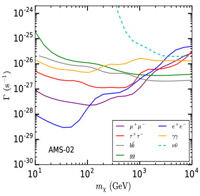
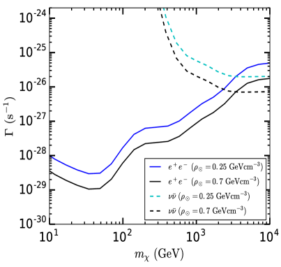
Figure 4: Top: Cosmic-ray positron flux measurement of AMS-02 is used to derive the 95% C.L. upper limits on $\Gamma$ assuming 100% branching ratio for each individual SM final state. The results are obtained for $D_{0}=2.7\times 10^{28}\,{\rm cm}^{2}{\rm s}^{-1}$, $\delta=0.6$, $z_{t}=4\,{\rm kpc}$ and $\rho_{\odot}=0.25\,{\rm GeV}\,{\rm cm}^{-3}$. Here, the results for seven DM decay modes are presented for illustration. Bottom: Variation of these upper limits on $\Gamma$ (for $e^{+}e^{-}$ and $\nu\bar{\nu}$ final states), with the diffusion parameters (bottom left panel) and the local DM density $\rho_{\odot}$ (bottom right panel) are shown. See the text for details.

In order to derive the $95\%$ C.L. upper limit on $\Gamma$ using the positron flux measured by AMS-02 we have adopted the methodology used in Ref. [84] to which the readers are referred for the details. Similar to Ref. [84], we assume the positron flux measured by AMS-02 arises solely from the astrophysical backgrounds and parameterize the $\log({\rm flux})$ as a degree 6 polynomial of $\log({\rm energy})$. The $\chi^{2}$ is defined as follows:

$$\chi^{2}=\sum_{i}\frac{\left(f^{model}_{i}(\alpha)-f^{data}_{i}\right)^{2}}{\sigma^{2}_{i}},$$ (2.11)

where $i$ represents each individual energy bin of AMS-02 with $f^{data}_{i}$ signifies the central value of the measured positron flux [53] and $f^{model}_{i}$ denotes the expected number of events in the $i$-th bin. $\sigma_{i}$ for each bin is obtained by adding the corresponding systematic and statistical uncertainties in quadrature [53]. Next we determine the best-fit values of the associated parameters by minimizing this $\chi^{2}$ and obtained the best-fit $\chi^{2}_{\rm bf}$. Then we add the DM induced positron flux to this modelled background $f^{model}_{i}(\alpha)$ and vary the parameters of this function ($\{\alpha\}$) within $30\%$ of their best-fit values without DM. The DM decay width $\Gamma$ is increased until the $\chi^{2}$ increases by 2.71 from its best-fit value:

$$\chi^{2}(\Gamma)=\chi^{2}_{\rm bf}+2.71,$$ (2.12)

so that the corresponding decay width gives the $95\%$ C.L. upper limit on $\Gamma$. Note that using the above-mentioned methodology we have recalculated the constraints for each individual SM final states for an annihilating WIMP and found that our limits match with the corresponding limits presented in Ref. [84].

From Eqn. 2.12, the $95\%$ C.L. upper limits on $\Gamma$ are obtained for $100\%$ branching ratio attributed to each individual channel. These limits are shown in the top panel of Fig. 4 where we have reported the limits obtained for seven illustrative decay modes of the DM assuming $D_{0}=2.7\times 10^{28}\,{\rm cm}^{2}{\rm s}^{-1}$, $\delta=0.6$, $z_{t}=4\,{\rm kpc}$ and $\rho_{\odot}=0.25\,{\rm GeV}\,{\rm cm}^{-3}$. For $m_{\chi}$ in the range $10\,{\rm GeV}$ to $\sim 2\,{\rm TeV}$, the constraints are most stringent for DM decays to electron and muon final states. For $m_{\chi}\gtrsim 2\,{\rm TeV}$, the positron spectra coming from $e^{+}e^{-}$ and $\mu^{+}\mu^{-}$ final states are highly energetic and fall outside the sensitivity range of AMS-02 and hence the corresponding limits weaken. We have also shown the limit for $\chi\rightarrow\nu\bar{\nu}$ channel and found that this decay mode is reasonably constrained for $m_{\chi}{\;\raise 1.29167pt\hbox{$>$\kern-7.5pt\raise-4.73611pt\hbox{$\sim$}}\;}4\,{\rm TeV}$ (see cyan line in Fig. 4; top panel). This is because, similar to the earlier cases, here, too, the resulting flux of positrons are comparable to the corresponding fluxes coming from other SM decay modes when $m_{\chi}$ is larger than a few TeV (see Fig. 1). DM decays to gluons and $b\bar{b}$ pairs are most weakly constrained for $m_{\chi}\sim 10\,{\rm GeV}$ - $100\,{\rm GeV}$, while the $\gamma\gamma$ is the least constrained channel for $m_{\chi}\sim 100\,{\rm GeV}$ - $4\,{\rm TeV}$.

In the bottom panel of Fig. 4 we have shown the variation of the upper limits on $\Gamma$ with the diffusion parameters (bottom left) and the local DM density (bottom right), respectively. Here, we have considered $e^{+}e^{-}$ and $\nu\bar{\nu}$ channels for the sake of illustration. In the bottom left panel, we have used two different sets of diffusion parameters, namely, $D_{0}=3.4\times 10^{27}\,{\rm cm}^{2}{\rm s}^{-1}$, $\delta=0.7$, $z_{t}=4\,{\rm kpc}$ (choice I; shown in black) and $D_{0}=2.3\times 10^{28}\,{\rm cm}^{2}{\rm s}^{-1}$, $\delta=0.46$, $z_{t}=15\,{\rm kpc}$ (choice II; shown in brown), in addition to our choice for these parameters which was mentioned earlier. Both of these choices are commonly used for the MW galaxy [115, 120, 121, 122]. From this figure it is evident that the limits obtained by us are quite robust against the variation of the diffusion parameters. In the bottom right panel, apart from our choice of $\rho_{\odot}=0.25\,{\rm GeV}\,{\rm cm}^{-3}$ we have also considered the maximum allowed value $\rho_{\odot}=0.7\,{\rm GeV}\,{\rm cm}^{-3}$ and shown the resulting limits for $e^{+}e^{-}$ and $\nu\bar{\nu}$ final states (black lines), since astronomical observations constrain $\rho_{\odot}$ in the range $0.25\,{\rm GeV}\,{\rm cm}^{-3}-0.7\,{\rm GeV}\,{\rm cm}^{-3}$ [119]. From this figure, it is clear that, as one increases $\rho_{\odot}$, the limits on $\Gamma$ strengthen and for our choice of $\rho_{\odot}=0.25\,{\rm GeV}\,{\rm cm}^{-3}$ one obtains the most conservative upper limits on $\Gamma$.

2.2.4 Super-Kamiokande constraints

In addition to photons and electrons-positrons, SM neutrinos are also produced as the end products of the DM decay cascades. Similar to the gamma-ray fluxes the neutrino fluxes induced by the DM decays, too, are proportional to $\Gamma$ for any given value of $m_{\chi}$. Therefore, the decay width for any chosen value of the DM mass is constrained by comparing the expected DM decay generated neutrino flux from any suitably chosen astrophysical target with the measured flux of the SM neutrinos. Among several neutrino observations, Super-Kamiokande [59] provides the strongest constraints in case of DM decays for $m_{\chi}$ less than a TeV . Assuming the DM decays to each individual SM final state with $100\%$ branching ratio we have derived the $90\%$ C.L. upper limits on $\Gamma$ using the neutrino flux data from the MW galaxy measured by the Super-Kamiokande collaboration [59].

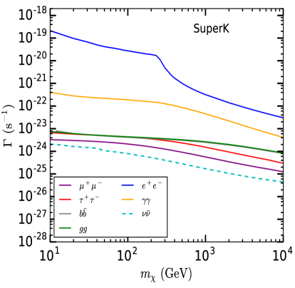
Figure 5: 90$\%$ C.L. upper limits on the DM decay width $\Gamma$ obtained using the measurement of the neutrino flux from the Milky Way (MW) galaxy by the Super-Kamiokande collaboration are shown for a 100$\%$ branching ratio attributed to each individual SM decay mode. Here the results for seven illustrative decay modes are shown.

In deriving these limits we have followed the ON-OFF procedure outlined in [59]. The ON and the OFF source regions are chosen exactly in accordance with Ref. [59]. The ON source region is a circular region centered around the galactic center (GC) with half-opening angle $80^{\circ}$ while the OFF source region is another circular region of the same size but offset by $180^{\circ}$ in Right Ascension with respect to the GC (see Ref. [59] for details). The neutrino+anti-neutrino flux distributions coming from the ON and the OFF source regions are obtained as follows:

$$\frac{d\Phi_{\rm ON,OFF}}{dE_{\nu}} = \,{\rm J}_{\rm ON,OFF}\frac{\Gamma}{4\pi\,m_{\chi}}\sum_{f}B_{f}\frac{2}{3}\,\frac{dN^{\nu}_{f}}{dE_{\nu}}(E_{\nu}),$$ (2.13)

where, $dN^{\nu}_{f}/dE_{\nu}$ represents the $\nu$ spectrum (same as the $\bar{\nu}$ spectrum) produced per DM decay to the SM final state $f$ and is obtained from [86, 110, 111, 112]. The factor of 1/3 in Eqn. 2.13 represents the fact that we have assumed $e,\mu$ and $\tau$ flavours are equally populated. The effect of the neutrino oscillation during the propagation throughout the galaxy is incorporated following the procedure described in Ref. [129]. In Eqn. 2.13, ${\rm J}_{\rm ON,OFF}$ are the astrophysical J-factors for the ON and the OFF source regions [59], respectively:

$$J_{\rm ON,OFF}=\underset{\Delta\Omega_{\rm ON,OFF}}{\int}d\Omega\underset{l.o.s}{\int}ds\,\rho_{d}(\vec{r}),$$ (2.14)

where the NFW profile $\rho_{d}(\vec{r})$ (given in Eqn. 2.9) is parameterized by $r_{s}=20\,{\rm kpc}$ and $\rho_{\odot}=0.3\,{\rm GeV\,cm}^{-3}$ [59, 130]. In Eqn. 2.14, $s$ is the line-of-sight ($l.o.s$) coordinate, $\Delta\Omega_{\rm ON,OFF}$ signify the solid angle subtended by the ON and the OFF source regions, respectively.

Thereafter, the number of upward going muon (UP$\mu$) type signal events ($N^{\rm UP\mu}_{\rm ON,OFF}$) and the number of contained muon events ($N^{\rm con}_{\rm ON,OFF}$) are calculated using the formulae provided in [85]. Following Ref. [59] detector livetimes of 4527 days for the UP$\mu$ events and 4223.3 days for the contained muon events have been assumed. The total number of signal events are thus given by $N_{\rm ON,OFF}=N^{\rm UP\mu}_{\rm ON,OFF}+N^{\rm con}_{\rm ON,OFF}$. The background flux of atmospheric neutrinos being isotropic the difference between the number of events expected from the ON and the OFF regions are essentially same as the difference between the number of expected signal events, i.e., $\Delta N=N_{\rm ON}-N_{\rm OFF}$. This number is then compared against the $90\%$ C.L. upper limit on the above-mentioned difference (provided in [59]) to derive the $90\%$ C.L. upper limit on $\Gamma$ as shown in Fig. 5.

In Fig. 5, the $90\%$ C.L. upper limits on $\Gamma$ for seven decay channels are shown. Note that, unlike other observations, here the constraint on $\chi\rightarrow\nu\bar{\nu}$ channel is the strongest one over the entire DM mass range considered (see Figs. 2, 3 and 4). This constraint is substantially stronger than those obtained from the previously considered observations for DM mass less than a few hundreds of GeV. This is because, in this case the neutrinos (anti-neutrinos) themselves are detected without relying on the photons or the electrons-positrons originating from them. On the other hand, for the $e^{+}e^{-}$ and $\gamma\gamma$ final states the detectable $\nu\,(\bar{\nu})$ come from the radiation of electroweak gauge bosons, which being suppressed the corresponding constraints are the weaker ones (shown by blue and orange lines in Fig. 5).

3 Analysis of existing data: a generic approach

We now proceed to derive new limits on the total DM decay width from existing astrophysical and cosmological data, allowing $\chi$ to decay into all possible SM particle pairs with arbitrary branching ratios. This is clearly different from most approaches taken so far, where constraints from different observations have been derived assuming $100\%$ branching ratio for each individual DM decay mode taken one at a time (see Sec. 2.2).

In a generic model of decaying scalar dark matter, the DM particle may in principle decay into multiple two-body SM final states with different branching ratios. These branching fractions are decided by the parameters of the model. In such cases, the DM decay induced fluxes of $\gamma$-rays, electrons (positrons) and neutrinos (antineutrinos) are obtained by summing over the fluxes arising from each individual channels weighted by their respective branching fractions. Thus the shapes of these resulting flux distributions are quite different from that obtained in the case of DM decays to a single SM final state with $100\%$ branching ratio. The spectral shapes of these distributions govern the bin-by-bin fluxes and thereby affect the constraints arising from different observations.

This is illustrated in Fig. 6, where, we have presented the photon spectra $dN^{\gamma}/dE$ (left panel) and the positron spectra $dN^{e^{+}}/dE$ (right panel) for two different branching ratio combinations of $b\bar{b}$, $\mu^{+}\mu^{-}$ and $\tau^{+}\tau^{-}$ final states, considering $m_{\chi}=500\,{\rm GeV}$. For combination 1, shown by the black dashed lines in each panel, equal branching fraction, i.e., $33.33\%$, is attributed to each individual DM decay mode. While, the magenta dashed lines are obtained for combination 2, for which we have assumed $5\%$ branching ratio to $b\bar{b}$, $25\%$ branching ratio to $\mu^{+}\mu^{-}$ and $70\%$ branching ratio to $\tau^{+}\tau^{-}$ channels. For comparison, we have also shown the corresponding spectra obtained for $100\%$ branching ratio to $b\bar{b}$ (gray solid line), $\mu^{+}\mu^{-}$ (purple solid line) and $\tau^{+}\tau^{-}$ (red solid line) final states. Clearly, in every energy bin, the fluxes predicted by these combinations are different from what one obtains for any particular final state with $100\%$ branching ratio and thus for each observation the resulting limits are also different. Also, note that the spectra obtained for combination 1 are quite different from those obtained for combination 2. This explains why the limit on the total decay width of the DM should be derived using these resulting flux distributions, the calculation of which requires a precise knowledge of the branching ratios of each allowed decay mode.

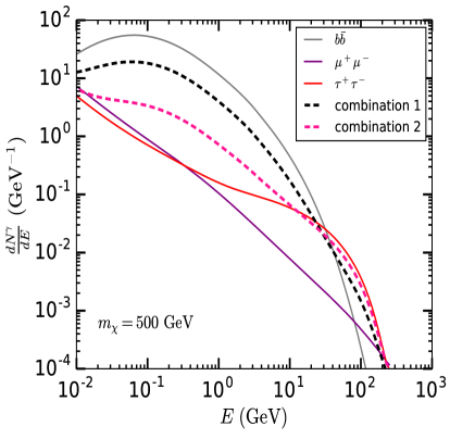
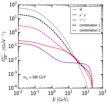
Figure 6: For $m_{\chi}=500\,{\rm GeV}$, the photon spectra $dN^{\gamma}/dE$ (left panel) and positron spectra $dN^{e^{+}}/dE$ (right panel) are shown for $b\bar{b}$ (gray solid line), $\mu^{+}\mu^{-}$ (purple solid line) and $\tau^{+}\tau^{-}$ (red solid line) final states assuming $100\%$ branching ratio for each individual channel. The corresponding energy distributions assuming equal branching fraction for each of the above-mentioned decay modes (black dashed lines) and the distributions obtained when $5\%$ branching ratio is attributed to $b\bar{b}$, $25\%$ branching ratio to $\mu^{+}\mu^{-}$ and $70\%$ branching ratio to $\tau^{+}\tau^{-}$ (magenta dashed lines) are also shown in each panel. See the text for details.

In fact, studies exist in the literature where DM decays are parameterized by higher-dimensional operators and constraints on the DM parameter space are derived assuming DM decays to all possible SM final states allowed by any given higher-dimensional operator [81]. In this case, branching ratio for any given decay mode is decided by the higher-dimensional operator which is responsible for the corresponding decay. However, it is possible to adopt a more general approach where one does not need to know the Lagrangian governing the DM interactions. For example, in the context of 2$\rightarrow$2 $s$-wave annihilations of a WIMP DM, Ref. [84] has derived a robust lower limit of $\sim 20\,{\rm GeV}$ on $m_{\chi}$ using the data of Planck CMB observation [4], AMS-02 positron flux measurement [53] and Fermi-LAT gamma-ray measurement from the dSph galaxies [131, 132]. In deriving this limit arbitrary branching fractions are assumed for each of the DM annihilation final states (excluding $\nu\bar{\nu}$). The most important conclusion of such study is substantial relaxation of the lower limit on $m_{\chi}$ which is otherwise of the order of $\sim 100\,{\rm GeV}$ when one considers DM annihilations to individual SM final states, e.g., $b\bar{b}$, $\tau^{+}\tau^{-}$, with 100$\%$ branching ratio. Motivated by this, here, we shall derive a robust constraint on the DM parameter space utilizing the data of Planck CMB [4], Fermi-LAT IGRB [46], AMS-02 positron [53] and Super-Kamiokande neutrino flux measurements [59] by allowing arbitrary branching fraction to each individual DM decay mode.

3.1 Analysis methodology

In order to derive the upper limit on the total decay width of $\chi$ that decays to all possible kinematically allowed two-body SM final states, i.e., $\chi\rightarrow$ ${\rm SM}_{1}$ $\mkern 1.5mu\overline{\mkern-1.5mu\rm SM\mkern-1.5mu}\mkern 1.5mu_{2}$ (as mentioned in Sec. 2.1) with arbitrary branching fractions we take the following steps:

• We have varied $m_{\chi}$ in the range 10 GeV - 10 TeV. For any given value of $m_{\chi}$, we scan over all possible branching ratio combinations of the kinematically allowed two-body SM final states ${\rm SM}_{1}$ $\mkern 1.5mu\overline{\mkern-1.5mu\rm SM\mkern-1.5mu}\mkern 1.5mu_{2}$, to derive the maximum allowed value of the total DM decay width. While scanning over the possible branching ratio combinations the branching fraction corresponding to each two-body SM final state is varied in the range 0$\%$ to 100$\%$ with an incremental change of $2\%$ in each successive step. Additionally, we have also ensured that for each such combination the branching fractions of all channels add up to unity.

• For any value of $m_{\chi}$ and specific branching ratio combination, we derive the 95$\%$ C.L. upper limits on $\Gamma$ for each individual observations following the procedures described in Sec. 2.2. Thus, given the $m_{\chi}$ and the branching ratio combination, we have three different upper limits on $\Gamma$ corresponding to Planck CMB [4], Fermi-LAT IGRB [46] and AMS-02 positron flux [53] measurements. The strongest among these upper limits represents the value of $\Gamma$ that is allowed by all the observations considered. In addition, when $\chi\rightarrow\nu\bar{\nu}$ is included in our analysis, the upper limit on $\Gamma$ coming from Super-Kamiokande neutrino flux measurement [59] is also taken into consideration.

• Given any $m_{\chi}$, for each branching ratio combination, we obtained the $\Gamma$ value that is consistent with all observations. The weakest one among these allowed values of $\Gamma$ obtained for different branching ratio combinations represents the maximum allowed value of the total DM decay width, i.e., $\Gamma_{\rm max}$, for the considered value of $m_{\chi}$. Therefore, there exists no branching ratio combination for which a value of $\Gamma>\Gamma_{\rm max}$ is allowed by the existing observational data. The branching ratio combination for which the allowed value of $\Gamma$ is the weakest, i.e., the combination corresponding to $\Gamma_{\rm max}$, is defined as the threshold branching ratio combination ($B_{f}$).

For any $m_{\chi}$ value $\Gamma_{\rm max}$ and $B_{f}$ together define the most weakly constrained decaying scalar DM scenario assuming DM decays to SM particle pairs only. The above-mentioned methodology is applied to derive $\Gamma_{\rm max}$ for four different situations:

• Case 1: DM decays to visible SM final states with arbitrary branching fractions, while the branching ratio of the $\nu\bar{\nu}$ final state is identically set to zero.

• Case 2: DM decays to all possible SM final states including $\nu\bar{\nu}$. In this case the branching fraction for the $\nu\bar{\nu}$ decay mode is also allowed to vary in the range 0$\%-100\%$.

• Case 3: DM decays to $\nu\bar{\nu}$ with exactly 50$\%$ branching ratio while the branching ratios of other SM decay modes are allowed to vary freely such that their branching ratios add up to 0.5. In this case, the incremental changes in the branching ratios of all non-neutrino SM final states are $1\%$ in each step.

• Case 4: DM decays to $\nu\bar{\nu}$ with 100$\%$ branching ratio and the branching ratios for all other decay modes are set to zero.

Actually, Case 3 and Case 4 are two sub-classes of Case 2. However, our results are very sensitive to the exact branching ratio of the $\nu\bar{\nu}$ final state and thus we have considered Case 3 and Case 4, separately.

In the next subsection, we present $\Gamma_{\rm max}$ for all of the aforementioned cases and the threshold branching fractions $B_{f}$ for Case 1 and Case 2.

3.2 General constraints on decaying DM

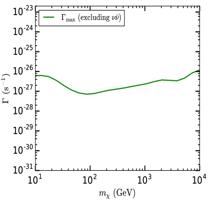
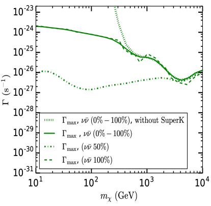
Figure 7: Left: Varying the branching ratios of all SM final states (excluding $\nu\bar{\nu}$) in the range $0\%-100\%$ and combining the data of Planck CMB, Fermi-LAT IGRB and AMS-02 positron observations the maximum allowed value of the total DM decay width, i.e., $\Gamma_{\rm max}$, is obtained for $m_{\chi}$ in the range 10 GeV - 10 TeV. For any $\Gamma>\Gamma_{\rm max}$ there exists no branching ratio combination which is allowed by all the aforementioned observations. Right: The branching ratio of $\nu\bar{\nu}$ final state is also varied in the range $0\%-100\%$ and the data of the above-mentioned observations are used along with the data of Super-Kamiokande neutrino flux measurement to obtain the $\Gamma_{\rm max}$ shown by the green solid line. The green dotted line is obtained without including the Super-Kamiokande data. Combining all four observations the green dashed dotted and the green dashed lines are derived which represent the $\Gamma_{\rm max}$ for DM decays to $\nu\bar{\nu}$ with precisely 50$\%$ and 100$\%$ branching ratios, respectively. See the text for details.

For the range of the DM masses we have studied, $\Gamma_{\rm max}$’s for the four above-mentioned cases are shown in Fig. 7 and the threshold branching fractions, $B_{f}$’s for Cases 1 and 2 are presented in Tab. 1 and in Fig. 8.

In the left panel of Fig. 7, we show $\Gamma_{\rm max}$ for Case 1 by the green solid line. In deriving this constraint we have used the data collected by Planck [4], Fermi-LAT [46] and AMS-02 [53]. Note that when we considered the DM decays to a single channel with 100$\%$ branching ratio the existing constraints are quite strong. For example, for decays to $\gamma\gamma$ final state one finds that $\Gamma{\;\raise 1.29167pt\hbox{$<$\kern-7.5pt\raise-4.73611pt\hbox{$\sim$}}\;}3\times 10^{-29}\,{\rm s}^{-1}$ is allowed for $m_{\chi}\sim 400\,{\rm GeV}$ (see Fig. 3), while for the $e^{+}e^{-}$ channel the upper limit on $\Gamma$ is $\sim 3\times 10^{-29}\,{\rm s}^{-1}$ for $m_{\chi}\sim 40\,{\rm GeV}$ (see Fig. 4). On the other hand, allowing arbitrary branching ratios to different channels relax the constraints substantially, e.g., $\Gamma{\;\raise 1.29167pt\hbox{$<$\kern-7.5pt\raise-4.73611pt\hbox{$\sim$}}\;}10^{-27}\,{\rm s}^{-1}$ is consistent with all observations for all values of $m_{\chi}$ in the range 10 GeV - 10 TeV (Fig. 7; left panel).

The limits for the Cases 2, 3 and 4 are shown in the right panel of Fig. 7. In obtaining the dotted line, the branching ratios of all decay channels including the $\chi\rightarrow\nu\bar{\nu}$ channel are varied in the range $0\%-100\%$ and the data of Planck CMB [4], Fermi-LAT IGRB [46] and AMS-02 positron flux [53] observations have been used. It is clear that, no upper limit on $\Gamma$ is obtained in this case, for DM masses below a few hundreds of GeV. This is because, for such values of $m_{\chi}$, the low energy $\nu\bar{\nu}$ pairs produced from DM decays give rise to highly suppressed $e^{-}$, $e^{+}$ and $\gamma$-ray spectra (see the discussion of Fig. 1), which are not detectable in any of the observations considered. For heavier DM particles, on the other hand, final state $\nu\bar{\nu}$ pairs are highly energetic and hence the fluxes of $e^{-}$, $e^{+}$ and $\gamma$ also become comparable to that coming from other SM final states (see Fig. 1). Thus, for such values of $m_{\chi}$, the constraint on the $\nu\bar{\nu}$ channel, become stronger than some of the other SM final states (see Figs. 3 and 4) and the maximum allowed $\Gamma$ also strengthens.

The situation changes when the data from the Super-Kamiokande observation [59] are also taken into account. In particular, for $m_{\chi}{\;\raise 1.29167pt\hbox{$<$\kern-7.5pt\raise-4.73611pt\hbox{$\sim$}}\;}250\,{\rm GeV}$, Super-Kamiokande constraint on the $\nu\bar{\nu}$ final state is considerably stronger (see Fig. 5) since in this case the final state $\nu\bar{\nu}$ pairs themselves are detected instead of the $e^{-}$, $e^{+}$ and $\gamma$ fluxes produced via electroweak radiation. Therefore, the resulting $\Gamma_{\rm max}$, shown by the green solid line (see Fig. 7; right panel) is stronger than what we obtained in the previous case, where we have used the data collected by Planck [4], Fermi-LAT [46], and AMS-02 [53], for $m_{\chi}{\;\raise 1.29167pt\hbox{$<$\kern-7.5pt\raise-4.73611pt\hbox{$\sim$}}\;}250\,{\rm GeV}$. Thus, including $\chi$ decays to $\nu\bar{\nu}$ pairs and taking Super-Kamiokande data into account, we obtain $\Gamma_{\rm max}\sim 10^{-26}\,{\rm s}^{-1}$ for $m_{\chi}{\;\raise 1.29167pt\hbox{$>$\kern-7.5pt\raise-4.73611pt\hbox{$\sim$}}\;}\mathcal{O}({\rm TeV})$ and $\Gamma_{\rm max}\sim 10^{-24}\,{\rm s}^{-1}$ for $m_{\chi}\sim 100\,{\rm GeV}$.

Comparing the solid lines in left and right panels of Fig. 7, one can clearly see that the inclusion of the $\nu\bar{\nu}$ final state changes $\Gamma_{\rm max}$ substantially. Therefore, in the right panel of Fig. 7, we also present $\Gamma_{\rm max}$ for Case 3 (dashed dotted line) and Case 4 (dashed line), respectively. In Case 3, sum of the branching fractions of the visible SM final states always equals 0.5 and the resulting fluxes of $e^{+}$($e^{-}$), $\gamma$ and $\nu(\bar{\nu})$ are added to half of the corresponding fluxes that would have come if the $\nu\bar{\nu}$ final state had $100\%$ branching ratio. Using these fluxes we then determine $\Gamma_{\rm max}$ using the data of Planck CMB [4], Fermi-LAT IGRB [46], AMS-02 positron [53] and Super-Kamiokande neutrino [59] observations. In this case, throughout the considered $m_{\chi}$ range, we obtain $\Gamma_{\rm max}\sim 10^{-26}\,{\rm s}^{-1}-10^{-27}\,{\rm s}^{-1}$ which is stronger than the limit obtained in Case 2, especially in the range $m_{\chi}\lesssim\mathcal{O}({\rm TeV})$. This is because, in this case, the observed fluxes always receive substantial contributions from the visible SM final states.

On the other hand, in Case 4, the fluxes of stable SM particles arise from the $\nu\bar{\nu}$ pairs produced in DM decays. Therefore, for any value of $m_{\chi}$ the strongest constraint on the $\nu\bar{\nu}$ final state dictate the $\Gamma_{\rm max}$ (dashed line in Fig. 7; right panel). Therefore, for $m_{\chi}{\;\raise 1.29167pt\hbox{$<$\kern-7.5pt\raise-4.73611pt\hbox{$\sim$}}\;}$ a few hundreds of GeV, $\Gamma_{\rm max}$ follows the Super-Kamiokande limit on the $\chi\rightarrow\nu\bar{\nu}$ channel (see Fig. 5) while for higher values of $m_{\chi}$, $\Gamma_{\rm max}$ is determined by the data of Planck [4], Fermi-LAT [46] and AMS-02 [53] observations. Note that $\Gamma_{\rm max}$ in this case is stronger than that obtained in Case 2 for $m_{\chi}{\;\raise 1.29167pt\hbox{$>$\kern-7.5pt\raise-4.73611pt\hbox{$\sim$}}\;}2\,{\rm TeV}$. This is because, for such masses Fermi-LAT and AMS-02 constraints on the $\nu\bar{\nu}$ final state are stronger than the corresponding constraints on some of the visible SM final states (see Figs. 3 and 4).

	$m_{\chi}$	$\Gamma_{\rm max}$	Threshold branching ratio $B_{f}$ ($\%$)
	(GeV)	$({\rm s}^{-1})$	$gg$	$b\bar{b}$	$\gamma\gamma$	$e^{+}e^{-}$	$\mu^{+}\mu^{-}$	$\tau^{+}\tau^{-}$	$W^{+}W^{-}$	$\nu\bar{\nu}$
	10	$6.1\times 10^{-27}$	$77.7$	$0$	$0$	$0$	$22.3$	$0$	-	-
	50	$1.0\times 10^{-27}$	$0$	$71.6$	$0$	$0$	$28.4$	$0$	-	-
	100	$7.4\times 10^{-28}$	$0$	$0$	$0$	$0$	$24.3$	$75.7$	-	-
	200	{ $\!\!1.1\times 10^{-27}$	$4.2$	$0$	$0$	$2.0$	$0$	$93.8$	$0$	-
		$1.5\times 10^{-27}$	$0$	$0$	$0$	$0$	$0$	$93.9$	$6.1$	-
Case 1	500	$1.6\times 10^{-27}$	$77.9$	$0$	$0$	$0$	$22.1$	$0$	$0$	-
	800	{ $\!\!2.1\times 10^{-27}$	$79.9$	$0$	$0$	$0$	$20.1$	$0$	$0$	-
		$2.0\times 10^{-27}$	$0$	$0$	$0$	$0$	$0$	$0$	$100$	-
	1000	{ $\!\!2.4\times 10^{-27}$	$71.7$	$0$	$0$	$0$	$28.3$	$0$	$0$	-
		$2.3\times 10^{-27}$	$9.9$	$0$	$0$	$0$	$0$	$0$	$90.1$	-
	1500	$3.2\times 10^{-27}$	$0$	$0$	$0$	$0$	$100$	$0$	$0$	-
	5000	{ $\!\!4.6\times 10^{-27}$	$0$	$69.2$	$30.8$	$0$	$0$	$0$	$0$	-
		$4.7\times 10^{-27}$	$0$	$0$	$10.3$	$0$	$0$	$0$	$89.7$	-
	10000	$1.2\times 10^{-26}$	$0$	$0$	$100$	$0$	$0$	$0$	$0$	-
	10	$2.0\times 10^{-24}$	$0$	$0$	$0$	$0$	$0$	$0$	-	$100$
	50	$1.1\times 10^{-24}$	$0$	$0$	$0$	$0$	$0$	$0$	-	$100$
	100	$7.8\times 10^{-25}$	$0$	$0$	$0$	$0$	$0$	$0$	-	$100$
	200	$5.0\times 10^{-25}$	$0$	$0$	$0$	$0$	$0$	$0$	$0$	$100$
Case 2	500	$1.1\times 10^{-25}$	$0$	$0$	$0$	$0$	$0$	$0$	$0$	$100$
	800	$5.8\times 10^{-26}$	$0$	$0$	$0$	$0$	$0$	$0$	$0$	$100$
	1000	$5.6\times 10^{-26}$	$0$	$0$	$0$	$0$	$0$	$0$	$0$	$100$
	1500	$3.5\times 10^{-26}$	$0$	$0$	$0$	$0$	$0$	$0$	$0$	$100$
	5000	{ $\!\!4.9\times 10^{-27}$	$0$	$69.2$	$30.8$	$0$	$0$	$0$	$0$	$0$
		$5.0\times 10^{-27}$	$0$	$0$	$10.2$	$0$	$0$	$0$	$89.8$	$0$
	10000	$1.3\times 10^{-26}$	$0$	$0$	$77.7$	$0$	$0$	$0$	$0$	$22.3$

Table 1: Branching fractions of each SM final state corresponding to the threshold branching ratio combination $B_{f}$ that decides $\Gamma_{\rm max}$ (tabulated in the third column), are shown for a few benchmark values of $m_{\chi}$ in the range 10 GeV - 10 TeV. In the upper half we present the results for Case 1, while in the lower half the branching ratio combinations obtained for Case 2 are shown. ‘-’ implies that the corresponding final state is not included while calculating $\Gamma_{\rm max}$.

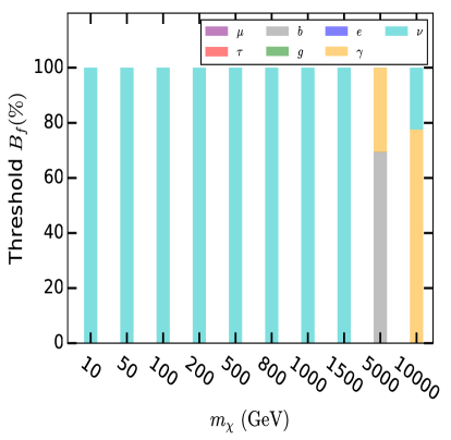
Figure 8: Left: One representative set of threshold branching ratio combinations ($B_{f}$’s) that correspond to the $\Gamma_{\rm max}$ obtained for Case 1, i.e., excluding the $\nu\bar{\nu}$ decay mode (shown in Fig. 7; left panel) are shown for various DM masses. Right: The threshold $B_{f}$’s (a representative set) for the $\Gamma_{\rm max}$ obtained in Case 2, i.e., when the branching ratio for $\chi\rightarrow\nu\bar{\nu}$ is also allowed to vary in the range $0\%-100\%$ and the data of all four observations are used, are presented (solid line in Fig. 7; right panel). See the text for details.

As we have discussed in Sec. 3.1, given any $m_{\chi}$ value, the threshold branching ratio combination is the one for which the allowed value of $\Gamma$ is the weakest one, i.e., $\Gamma_{\rm max}$ (shown in Fig. 7). It is evident that this threshold combination may be different for different values of $m_{\chi}$. In fact, for any given $m_{\chi}$, the threshold branching ratio combination need not be unique. There may in principle be more than one combinations of branching fractions which give nearly similar values of $\Gamma_{\rm max}$ for a given $m_{\chi}$. In this sense, the maximum allowed values of the total DM decay width (shown in Fig. 7) are quite robust. In Tab. 1, the threshold branching ratio combinations as obtained by us are reported for Case 1 and Case 2.

In the upper half of Tab. 1, we have presented the threshold branching ratio combinations for a few benchmark values of $m_{\chi}$ in the range 10 GeV - 10 TeV, considering Case 1. It is clear that, for several benchmark values of $m_{\chi}$, one obtains more than one different branching ratio combinations which yield very similar values of $\Gamma_{\rm max}$ (see third column of Tab. 1). Such cases are grouped under the curly braces in Tab. 1. Note that, in this case, for $m_{\chi}\sim\mathcal{O}(10{\,\rm TeV})$, $\gamma\gamma$ final state dominates the threshold branching ratio combination, since this is the least constrained channel by the Fermi-LAT data in this DM mass range (see Fig. 3). One representative threshold branching ratio combination for each of the $m_{\chi}$ values are also shown in Fig. 8 (left panel).

In the lower half of Tab. 1, the threshold branching ratio combinations for a few benchmark $m_{\chi}$ values are shown for Case 2. Here, too, the threshold branching ratio combination is not necessarily unique for any given $m_{\chi}$. As an example, for $m_{\chi}=5\,$TeV, we obtain two different branching ratio combinations which give similar values for $\Gamma_{\rm max}$ (see Tab. 1). In this case, a generic feature is that, for $m_{\chi}$ up to $\sim 1.5$ TeV, threshold branching ratio combinations are dominated by the $\nu\bar{\nu}$ channel, while for larger $m_{\chi}$, contribution of the $\nu\bar{\nu}$ final state to the threshold $B_{f}$ gradually decreases. This is because, $\nu\bar{\nu}$ is the least constrained final state for $m_{\chi}\lesssim\mathcal{O}$(TeV), while, for heavier DM particles Fermi-LAT and AMS-02 constraints on the $\nu\bar{\nu}$ channel are stronger than those obtained for several other decay modes (see Figs. 3 and 4). A representative set of threshold branching ratio combination for this case is shown in Fig. 8; right panel.

4 Radio signals at the SKA

In this section, we start with a brief discussion of the generation of radio signals from the DM decays occurring inside the dSph galaxies [133, 70, 71, 134, 135]. It is possible to detect such radio signals in the upcoming SKA radio telescope. Our goal is to classify the DM parameter space allowed by the existing observational data, into three distinct regions: detectable for all possible branching ratio combinations, detectable for specific combinations of branching fractions and non-detectable, assuming 100 hours of observation at the SKA. Thus in the next part we go ahead to describe the methodology we have adopted for such categorization.

4.1 Synchrotron radiation from dwarf spheroidal galaxies: a quick review

The SM particles produced from the decay of the DM particles within a galactic structure give rise to $e^{+}e^{-}$ pairs via their cascade decays. These $e^{+}(e^{-})$ act as the source of radio synchrotron signals due to their interaction with the magnetic field of the galaxy. The ultrafaint dSph galaxies are the most convenient targets to look for such DM induced radio signals. Their low star formation rates help in reducing the backgrounds stemming from various unknown astrophysical processes while high mass-to-light ratios (pointing towards a greater abundance of dark matter inside them) and closeness to our MW galaxy make them the most widely used targets for studying the DM induced radio signals [133, 70, 71, 76, 72, 77, 78, 136, 81]. To present our results, we consider the dSph Segue 1 (Seg 1) which is only $\sim 23\,{\rm kpc}$ away from the Sun and has a significantly high mass-to-light ratio (a few thousands times the value estimated for the Sun) that makes it one of the “darkest” dSph galaxy found till date [137, 138].

The electrons and the positrons produced from the cascade decays of the primary DM decay products propagate through the interstellar medium of the parent galaxy facing spatial diffusion and also energy loss by means of various electromagnetic processes. The equilibrium distribution of such electron (positron) $\left(\frac{dn_{e}}{dE}(E,\vec{r})\right)$ can be obtained by solving the following transport equation [139, 133, 134, 135, 140, 70]:

$$D(E)\nabla^{2}\left(\frac{dn_{e}}{dE}(E,\vec{r})\right)+\frac{\partial}{\partial E}\left(b(E)\frac{dn_{e}}{dE}(E,\vec{r})\right)+Q_{\chi}(E,\vec{r})=0,$$ (4.1)

where we assume that the $e^{+}$($e^{-}$) distribution reaches a steady state which in general holds for systems such as dwarf galaxies where the typical timescales required for the alterations of the DM density and the propagation parameters are large enough compared to the propagation timescale itself [110].

The term $b(E)$ in Eqn. 4.1 is the energy loss term for the $e^{+}$($e^{-}$) and is given by [139, 135, 134],

$$b(E) = b^{0}_{\rm IC}\left(\frac{E}{\rm GeV}\right)^{2}+b^{0}_{\rm Synch}\left(\frac{E}{\rm GeV}\right)^{2}\left(\frac{B}{\mu{\rm G}}\right)^{2}+b^{0}_{\rm Coul}n_{e}\left[1+\frac{1}{75}\log\left(\frac{E/m_{e}}{n_{e}}\right)\right]$$ (4.2)

$$+b^{0}_{\rm Brem}n_{e}\left[0.36+\log\left(\frac{E/m_{e}}{n_{e}}\right)\right],$$

with $b^{0}_{\rm IC}\simeq 0.25\times 10^{-16}\,{\rm GeV\,s}^{-1}$, $b^{0}_{\rm Synch}\simeq 0.0254\times 10^{-16}\,{\rm GeV\,s}^{-1}$, $b^{0}_{\rm Coul}\simeq 6.13\times 10^{-16}\,{\rm GeV\,s}^{-1}$ and $b^{0}_{\rm Brem}\simeq 1.51\times 10^{-16}\,{\rm GeV\,s}^{-1}$ [139, 135, 134]. Here $m_{e}$ and $n_{e}$ ($\approx 10^{-6}$ [133]) denote the electron mass and the value of the average thermal electron density inside a dSph, respectively. As can be seen from Eqn. 4.2, for electron (positron) energies $E\gtrsim 1$ $\rm GeV$, the terms $b^{0}_{\rm IC}$ and $b^{0}_{\rm Synch}$ dominate. Note that since the synchrotron energy loss term is proportional to the square of the ambient magnetic field strength $B$, the $e^{+}(e^{-})$ loose more energy via synchrotron radiation while propagating through the region of high $B$-field.

Due to the lack of gas and dust particles, the magnetic field strengths of the ultrafaint dSphs are hardly known and are also difficult to constrain using experiments involving polarization measurements. However, there are various astrophysical effects which may give rise to significant contributions to the magnetic field strengths inside the local dSphs. In fact, a number of theoretical arguments have been proposed which predict for the values of $B$ at the $\mu{\rm G}$ level. For example, it is sometimes argued that the trend of falling of the magnetic field strength inside the MW galaxy, as one moves from the center towards the outskirts, can be linearly extrapolated to nearby dSph galaxies, leading to $B{\;\raise 1.29167pt\hbox{$>$\kern-7.5pt\raise-4.73611pt\hbox{$\sim$}}\;}1\,\mu{\rm G}$ at the location of Seg 1. Such an assumption is based on the observations of giant magnetized outflows from the central region of the MW galaxy, which point towards a $B$-field value larger than 10 $\mu{\rm G}$ at a distance of $\sim$ 7 kpc from the Galactic plane [141]. In addition, it is also possible that the dwarf galaxies have their own magnetic fields. For further details, readers are referred to Ref. [142].

For most part of our analysis we consider the magnetic field $B=1\,\mu{\rm G}$ for Seg 1 [133, 70, 71], but at the same time present our results for a smaller (and hence more conservative) value of $B=0.1\,\mu{\rm G}$.

The diffusion term $D(E)$ in Eqn. 4.1, on the other hand, can be parameterized as [71, 135, 70]:

$$D(E)=D_{0}\left(E/{\rm GeV}\right)^{\gamma},$$ (4.3)

where $D_{0}$ is the diffusion coefficient for the considered dSph and $\gamma$ is the corresponding diffusion index. If the value of $D_{0}$ is smaller, the electrons-positrons loose sufficient energy via synchrotron radiation before escaping from the diffusion zone of the dSph galaxy and hence the resulting radio signals are larger [78].

Similar to the case of the magnetic field strengths, the diffusion parameters, i.e., $D_{0}$ and $\gamma$, too, are barely constrained for ultrafaint dSphs because of their low luminosity. However, analogous to galactic clusters [143, 144] one may expect inside a dSph $D_{0}\propto V\times L$, where $V$ and $L$ represent the velocity of the stochastic gas motions and the associated characteristic length scale, respectively. Taking the above-mentioned parameterization, Ref. [145] has shown that the scaling of virial velocity dispersions in ultrafaint dSphs with respect to the value corresponding to the MW galaxy can be used to infer that, $D_{0}$ for a dSph is either of the same order of magnitude as its value for the Milky Way or smaller by an order of magnitude.

In the context of the dSph galaxy considered in this work, we choose $\gamma=0.7$ [145, 70, 71, 135] (in analogy with its value used for the MW galaxy [115]) and use mostly the value $D_{0}=3\times 10^{28}\,{\rm cm}^{2}\,{\rm s}^{-1}$ which is almost of the same order or one order of magnitude higher than the value often predicted for the Milky Way [115]. In parallel, we have also shown our results for a more conservative choice of $D_{0}$, i.e., $D_{0}=3\times 10^{29}\,{\rm cm}^{2}\,{\rm s}^{-1}$. All the combinations of the diffusion coefficient $D_{0}$ and the magnetic field $B$ assumed for the Seg 1 dSph in this work are still allowed by the existing radio observations [70, 71]. The diffusion zone of the Seg 1 dSph has been considered to be spherically symmetric with a radius $r_{h}=1.6\,{\rm kpc}$ [71].

The $e^{+}$($e^{-}$) source function $Q_{\chi}(E,\vec{r})$ (in Eqn. 4.1), which results from the decay of DM particles inside the target dSph halo, is given by [72, 81, 79],

$$Q_{\chi}(E,\vec{r})=\frac{\Gamma}{m_{\chi}}\sum_{f}\,B_{f}\,\frac{dN^{e^{+}}_{f}}{dE}(E)\rho_{d}(\vec{r}).$$ (4.4)

As mentioned earlier, $dN^{e^{+}}_{f}/dE$ is the energy spectrum of the $e^{+}$ (and equivalently $e^{-}$) produced per DM decay for the SM final state (channel) $f$. For the dSph Seg 1, $\rho_{d}(\vec{r})$ is assumed to follow the Einasto profile [146, 135]:

$$\rho_{d}(\vec{r})=\rho_{s}\,\exp\,\left\{-\frac{2}{\alpha}\left[\left(\frac{r}{r_{s}}\right)^{\alpha}-1\right]\right\},$$ (4.5)

where the associated parameters $\rho_{s}$, $r_{s}$ and $\alpha$ are set at the values used in [71, 135, 147].

Now that all terms in Eqn. 4.1 are given, one can solve this equation using the Green’s function method outlined in [139, 78, 133]. The solution of Eqn. 4.1, i.e., $\frac{dn_{e}}{dE}(E,\vec{r})$, is then used to obtain the radio synchrotron flux $S_{\nu}$ (resulting from electrons and positrons) as a function of the radio frequency ($\nu$):

$$S_{\nu}(\nu)=\frac{1}{4\pi}\int_{\Delta\Omega}d\Omega\int_{l.o.s}ds\left(2\int_{m_{e}}^{m_{\chi}/2}dE\frac{dn_{e}}{dE}(E,r(s,\Omega))P_{\rm Synch}(\nu,E,B)\right),$$ (4.6)

where $P_{\rm Synch}(\nu,E,B)$ is the synchrotron power spectrum corresponding to the $e^{-}$($e^{+}$) with an energy $E$ in a magnetic field $B$ (for the analytic form of the synchrotron power spectrum see [139, 133, 134]), $s$ is the line-of-sight ($l.o.s$) coordinate and $\Delta\Omega$ denotes the size of the emission region of the considered dSph. In the forthcoming sections, the observational prospects of DM decay induced radio signals from the Seg 1 dSph will be studied in the context of the SKA radio telescope [82].

4.2 Projection for the SKA

Apart from several other fields of cosmology and astrophysics, in understanding the properties of dark matter, too, the upcoming SKA is expected to play a pivotal role [76, 148, 149]. SKA operates over a large frequency range, i.e., 50 MHz - 50 GHz, which helps in constraining the DM parameter space for a wide range of DM masses. The inter-continental baseline lengths of the SKA allow one to efficiently resolve the astrophysical foregrounds and thereby enhances its capability. In addition, a higher surface brightness sensitivity is possible to achieve because of its large effective area compared to any other existing radio telescope [82].

This work being focused on studying the DM induced diffuse radio synchrotron signals from the dSph galaxies, the SKA sensitivity corresponding to the surface brightness is calculated and compared with the predicted radio signal. In order to estimate the approximate values of the sensitivity we have utilized the presently accepted baseline design given in the documents provided in the SKA website [82]. In order to do this estimation we have adopted the methodology provided in [78] and the rms noise in observations has been evaluated utilizing the formula given in [150]. Assuming 100 hours of observation time this estimate suggests that the SKA surface brightness sensitivity in the frequency range 50 MHz - 50 GHz is $10^{-6}$ - $10^{-7}$ Jy with a bandwidth of 300 MHz [82, 76, 77]. Such values of the surface brightness sensitivity facilitate the observations of very low energy radio signals coming from the ultrafaint dSphs.

The potential of the SKA telescope in detecting the radio signals originating from DM annihilations/decays is quite promising [76, 77, 78, 79, 80, 81]. As mentioned previously, here the detection prospects of the radio signals (in the frequency range $\sim$50 MHz to $\sim$50 GHz) produced from DM decays occurring inside the Seg 1 dSph are investigated assuming 100 hours of observation time at the SKA. Following Ref. [78], we define the SKA threshold sensitivity, which determines the minimum radio flux required for detection at the SKA, to be three times above the noise level or the sensitivity level [82], so that the possibility of any spurious noise feature being misinterpreted as a potential DM decay signal is reduced and the detection of the DM decay induced radio signal, if any, is statistically significant.

The radio signal predicted for the SKA has been estimated assuming that the SKA field of view is larger than the size of the considered dSph. As a result, the expected signal at the SKA receives contributions from the entire dSph. Such an assumption need not be true for radio telescopes like the Murchison Widefield Array (MWA) which is one of the precursors of the SKA. In these kind of telescopes the effect of the primary beam size is also needed to be taken into account while calculating the predicted signal [136].

4.2.1 Detectability at the SKA: methodology

Following our discussions in Sec. 3, we know that, for any $m_{\chi}$ value, the upper limit of the allowed part of the DM parameter space is set by $\Gamma_{\rm max}$ (shown in the left and the right panels of Fig. 7). Hence, for any given $m_{\chi}$ (in the range 10 GeV - 10 TeV) and $\Gamma$ ($\leq\Gamma_{\rm max}$), we scan over all possible branching ratio combinations of the kinematically allowed two-body SM final states, i.e., $\chi\rightarrow$ ${\rm SM}_{1}$ $\mkern 1.5mu\overline{\mkern-1.5mu\rm SM\mkern-1.5mu}\mkern 1.5mu_{2}$ (${\rm SM}_{1}$ $\mkern 1.5mu\overline{\mkern-1.5mu\rm SM\mkern-1.5mu}\mkern 1.5mu_{2}$ are defined in Sec. 2.1). In this scan, the branching fraction for each individual DM decay mode is varied between $0\%$ to $100\%$ with an incremental change of $2\%$ in each consecutive step (similar to what we have done in Sec. 3). For the given $m_{\chi}$ and $\Gamma$ each such combination represents a different DM model. If the radio flux ($S_{\nu}$) for any particular branching ratio combination is above the SKA sensitivity level (corresponding to a given observation time) in at least one frequency bin, then DM decay to that particular final state is detectable at the SKA for the considered time of observation.

For a given ($m_{\chi}$, $\Gamma$) set lying in the allowed region of the DM parameter space, we first obtain the maximum radio flux ($S^{\rm max}_{\nu}$) and the minimum radio flux ($S^{\rm min}_{\nu}$) in every frequency bin in the range 30 MHz to 100 GHz by scanning over all possible branching ratio combinations of the DM decay modes and hence the combinations of branching fractions that give rise to $S^{\rm max}_{\nu}$ (or $S^{\rm min}_{\nu}$) may be different in each frequency bin. Note that in any frequency bin the branching ratio combination that gives $S^{\rm max}_{\nu}$ (or $S^{\rm min}_{\nu}$) is independent of the chosen value of $\Gamma$ and though, $S^{\rm max}_{\nu}$ (or $S^{\rm min}_{\nu}$) itself changes with $\Gamma$, the corresponding branching ratio combination remains the same.

In each bin, the radio fluxes ($S_{\nu}$) associated with all branching ratio combinations always lie between $S^{\rm max}_{\nu}$ and $S^{\rm min}_{\nu}$. Therefore, depending on these maximum and minimum radio fluxes, one can determine whether the chosen ($m_{\chi}$, $\Gamma$) point is detectable or non-detectable at the SKA. The DM models which are detectable at the SKA can be further categorized into two classes. The first one represents the scenarios which are detectable for all possible branching ratio combinations while the second one is composed of the DM models which are detectable only for certain specific branching ratio combinations of the DM decay modes.

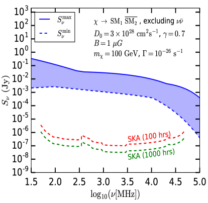
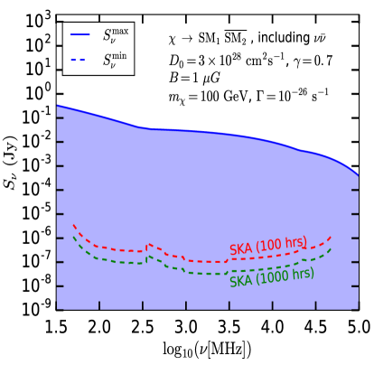
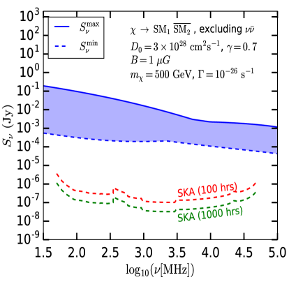
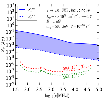
Figure 9: Considering the Seg 1 dSph as the target, the maximum ($S^{\rm max}_{\nu}$) and the minimum ($S^{\rm min}_{\nu}$) radio synchrotron flux distributions (the blue solid and the blue dashed lines, respectively) are shown as functions of the radio frequency $\nu$ in the range $30\,$MHz to $100\,$GHz, for $m_{\chi}=100\,{\rm GeV}$ (top panel) and $m_{\chi}=500\,{\rm GeV}$ (bottom panel). In each panel, the radio fluxes ($S_{\nu}$) for all branching ratio combinations fall within the blue shaded region. The results excluding $\chi\rightarrow\nu\bar{\nu}$ are shown in the left panel while that including the $\nu\bar{\nu}$ decay mode with the corresponding branching ratio varied between 0$\%$ and 100$\%$ are presented in the right panel. In all cases, an illustrative value of the DM decay width $\Gamma=10^{-26}\,{\rm s}^{-1}$ have been used. We have taken $D_{0}=3\times 10^{28}\,{\rm cm}^{2}\,{\rm s}^{-1}$, $\gamma=0.7$ and $B=1\mu{\rm G}$ in this figure. The SKA sensitivity curves for 100 hours (red dashed lines) and 1000 hours (green dashed lines) of observation times are also presented. See the text for details.

Considering Seg 1 dSph as the source, in Fig. 9, we show $S^{\rm max}_{\nu}$ (blue solid line) and $S^{\rm min}_{\nu}$ (blue dashed line) as functions of the radio frequency $\nu$ in the range $\sim$30 MHz to $\sim$100 GHz for two representative values of the DM mass, i.e., $m_{\chi}=100\,{\rm GeV}$ (top panel) and $m_{\chi}=500\,{\rm GeV}$ (bottom panel). $S_{\nu}$ for all branching ratio combinations lie within the blue shaded region. Here we have assumed $D_{0}=3\times 10^{28}\,{\rm cm}^{2}\,{\rm s}^{-1}$, $\gamma=0.7$ and $B=1\mu{\rm G}$. In the left panel we have shown the fluxes for Case 1 (mentioned in Sec. 3) while in the right panel Case 2 (as defined in Sec. 3) is considered. Both of the chosen $m_{\chi}$ values, i.e., $100\,{\rm GeV}$ and $500\,{\rm GeV}$, are well within the DM mass range we are focusing on, i.e., 10 GeV - 10 TeV and have additional motivations when one takes $\chi\rightarrow\nu\bar{\nu}$ channel into account, which will be evident from the following discussions. In each of the cases considered, we have chosen $\Gamma=10^{-26}\,{\rm s}^{-1}$ for illustration. In addition, the SKA sensitivities for 100 hours (red dashed line) and 1000 hours (green dashed line) of observation times are also presented. Note that the SKA noise goes as inverse of the square root of the observation time and thus the sensitivity corresponding to 1000 hours of observation time is enhanced nearly by a factor of three compared to that obtained for 100 hours of observation time [78]. This is the reason why the green dashed line lies a factor of three below the red dashed line in Fig. 9.

In the top left panel of Fig. 9, we have shown the radio flux distributions for $m_{\chi}=100\,{\rm GeV}$ and $\Gamma=10^{-26}\,{\rm s}^{-1}$ assuming Case 1, i.e., DM decay to $\nu\bar{\nu}$ final state is not included. For a radio frequency of $\sim 1\,{\rm GHz}$, the maximum flux is obtained when $\chi$ dominantly decays into $\mu^{+}\mu^{-}$ while DM decays to $Z\gamma$, $\gamma\gamma$ or any of their combinations give rise to $S^{\rm min}_{\nu}$. As mentioned earlier, the branching ratio combinations that correspond to $S^{\rm max}_{\nu}$ (or $S^{\rm min}_{\nu}$) are not the same in every frequency bin. As an example, for $\nu\sim 100\,{\rm MHz}$, $q\bar{q}$, $b\bar{b}$, $gg$ final states or any of their combinations give $S^{\rm max}_{\nu}$, and for DM decays into $\gamma\gamma$, $e^{+}e^{-}$ final states or any of their combinations, one obtains the minimum radio flux. For our chosen value of $\Gamma$ both $S^{\rm max}_{\nu}$ and $S^{\rm min}_{\nu}$ are above the SKA sensitivity curves in all frequency bins and thus the radio fluxes for all possible branching ratio combinations are also above the SKA sensitivity levels everywhere in the considered frequency range. Therefore, this combination of $(m_{\chi},\Gamma)$ is detectable at the SKA (in both 100 hours and 1000 hours of observations) for all possible branching ratio combinations. Although in this case the radio fluxes are above the SKA sensitivity levels in all frequency bins, it may also happen that $S_{\nu}$ go above the SKA sensitivity level over a certain frequency range, in which case the corresponding radio signals are detectable in that frequency range only. For example, if $\Gamma$ is reduced roughly by three orders, radio signals for all branching ratio combinations are above the SKA sensitivity levels only in the frequency range $60\,{\rm MHz}-13\,{\rm GHz}$, and hence this $(m_{\chi},\Gamma)$ point, too, is detectable at the SKA for all possible combinations of the DM decay modes.

Now if one scales down $\Gamma$ at least by four orders of magnitude both $S^{\rm max}_{\nu}$ and $S^{\rm min}_{\nu}$ decrease by the same amount and consequently, $S^{\rm max}_{\nu}$ is still above the SKA sensitivity levels everywhere but $S^{\rm min}_{\nu}$ falls below the SKA sensitivity curve obtained for 100 hours of observation time (red dashed line), in all frequency bins. As a result, the red dashed curve lies within the blue shaded region, which implies that, $S_{\nu}$ for certain branching ratio combinations are still above the SKA sensitivity level (for 100 hours of observation) while that for other branching ratio combinations are below the sensitivity level. Therefore, such a value of $(m_{\chi},\Gamma)$ is detectable in the 100 hours of observation at the SKA depending on the branching ratio combination of the DM decay mode. If $\Gamma$ is further decreased by a factor of 50, both $S^{\rm max}_{\nu}$ and $S^{\rm min}_{\nu}$ will go below the sensitivity level corresponding to 100 hours of the observation time, in all frequency bins. As a result, there exist no branching ratio combination for which the resulting $S_{\nu}$ is above the SKA sensitivity level. This $(m_{\chi},\Gamma)$ combination is never detectable in 100 hours of observation at the SKA.

On the other hand, each time, had $\Gamma$ been reduced by an extra factor of three, first $S^{\rm min}_{\nu}$ and then in the next time $S^{\rm max}_{\nu}$ would have gone below the green dashed line. Therefore, the resulting $(m_{\chi},\Gamma)$ points are branching ratio dependently detectable and non-detectable, respectively, in the 1000 hours of observation at the SKA. The origin of this factor of three can be understood from the relative difference between the sensitivity levels obtained for 100 hours and 1000 hours of observation times (the red and the green dashed curves in Fig. 9).

In the bottom left panel of Fig. 9 (here, too, $\chi\rightarrow\nu\bar{\nu}$ is not included) results are shown for the parameter point $m_{\chi}=500\,{\rm GeV}$, $\Gamma=10^{-26}\,{\rm s}^{-1}$. In this case, for $\nu\sim 1\,{\rm GHz}$, the branching ratio combination that gives $S^{\rm max}_{\nu}$ is determined by $q\bar{q}$, $b\bar{b}$, $gg$, $t\bar{t}$ channels, while $S^{\rm min}_{\nu}$ is obtained when $\chi$ decays dominantly into $e^{+}e^{-}$ pairs. Both $S^{\rm max}_{\nu}$ and $S^{\rm min}_{\nu}$ are above the SKA sensitivity levels throughout the considered frequency range and thus this $(m_{\chi},\Gamma)$ point is detectable at the SKA for all possible branching ratio combinations. However, in this case if $\Gamma$ is decreased by nearly three orders the resulting ($m_{\chi},\Gamma$) point becomes detectable at the SKA (100 hours) for certain specific branching ratio combinations of the DM decay modes and becomes non-detectable when $\Gamma$ is further decreased by a factor of 100.

As mentioned earlier, the radio fluxes for Case 2, i.e., including the $\nu\bar{\nu}$ decay mode (with arbitrary branching fraction in the range $0\%-100\%$) are presented in the right panel of Fig. 9. Note that for $m_{\chi}=100\,{\rm GeV}$ and $\Gamma=10^{-26}\,{\rm s}^{-1}$ (Fig. 9; top right panel), the maximum radio flux distribution is similar to that obtained excluding $\nu\bar{\nu}$ final state (see Fig. 9; top left panel). In fact, as in Case 1, here, too, for a radio frequency of $\sim 1\,{\rm GHz}$, $S^{\rm max}_{\nu}$ corresponds to DM decays to $\mu^{+}\mu^{-}$. For this ($m_{\chi}$, $\Gamma$) point $S^{\rm max}_{\nu}$ always lies above the SKA sensitivity curves. However, the minimum radio flux is now much below the SKA sensitivity levels. This is because, throughout the frequency range, $S^{\rm min}_{\nu}$ is obtained when $\nu\bar{\nu}$ is the dominant decay mode.

Following our earlier discussions, we know that, for DM mass less than a few hundreds of GeV, the fluxes of $e^{+}(e^{-})$ produced from the $\nu\bar{\nu}$ final state are significantly suppressed (see the discussions of Fig. 1). Thus the resulting radio signals are also negligibly small for all reasonable values of $\Gamma$. As a result, for the considered ($m_{\chi},\Gamma$) point $S^{\rm min}_{\nu}$ lies below the SKA sensitivity levels everywhere. Clearly, this ($m_{\chi},\Gamma$) point is detectable at the SKA only for certain specific branching ratio combinations. Reduction in $\Gamma$ by nearly five orders of magnitude causes $S^{\rm max}_{\nu}$ to go below the red dashed curve and hence the resulting ($m_{\chi},\Gamma$) point becomes non-detectable in the 100 hours of observation at the SKA. Note that if $\Gamma$ is reduced by an extra factor of three, the resulting ($m_{\chi},\Gamma$) point is non-detectable even in the 1000 hours of observation at the SKA.

On the other hand, for $m_{\chi}=500\,{\rm GeV}$ and $\Gamma=10^{-26}\,{\rm s}^{-1}$ (bottom right panel of Fig. 9) both $S^{\rm max}_{\nu}$ and $S^{\rm min}_{\nu}$ are above the SKA sensitivities in all frequency bins. Similar to Case 1 (shown in Fig. 9; bottom left panel), $S^{\rm max}_{\nu}$ in the $\nu\sim 1\,{\rm GHz}$ bin is obtained for DM decays to $q\bar{q}$, $b\bar{b}$, $gg$, $t\bar{t}$ final states or any of their combinations. On the other hand, in the same frequency bin, though, $S^{\rm min}_{\nu}$ is obtained when DM decays dominantly into $\nu\bar{\nu}$, in this case, the DM being heavier, the final state $\nu\bar{\nu}$ pairs are comparatively more energetic. Therefore, the resulting fluxes of $e^{+}(e^{-})$ coming from the $\nu\bar{\nu}$ final state are comparable to that obtained for other SM final states (see Fig. 1) which leads to an enhancement of the associated radio signals. Therefore, the chosen ($m_{\chi},\Gamma$) point is detectable at the SKA for all possible branching ratio combinations. Approximately three (five) orders decrease in $\Gamma$ suppresses the radio fluxes in a way such that the resulting ($m_{\chi},\Gamma$) points are detectable for certain branching ratio combinations (non-detectable) in the 100 hours of observation at the SKA.

Note that the value $\Gamma=10^{-26}\,{\rm s}^{-1}$ chosen here, is allowed by the existing astrophysical and cosmological data when $\chi\rightarrow\nu\bar{\nu}$ is included in the analysis (see Fig. 7; right panel). For the analysis performed excluding $\nu\bar{\nu}$, $\Gamma=10^{-26}\,{\rm s}^{-1}$ represents an illustrative value. Therefore, in this case, while determining the SKA detectability one needs to choose the value of $\Gamma$ appropriately so that the resulting $\Gamma$ is allowed by the existing observations (see Fig. 7; left panel).

4.2.2 SKA detectability criteria: a summary

Therefore, for any given ($m_{\chi},\Gamma$) point, scanning over all possible branching ratio combinations of the DM decay modes, one obtains $S^{\rm max}_{\nu}$ and $S^{\rm min}_{\nu}$ in every frequency bin. Depending on the distributions of $S^{\rm max}_{\nu}$ and $S^{\rm min}_{\nu}$, the detectability (for a given observation time at the SKA) of any ($m_{\chi},\Gamma$) point lying in the allowed part of the $m_{\chi}-\Gamma$ plane is decided by the following considerations:

• If both $S^{\rm max}_{\nu}$ and $S^{\rm min}_{\nu}$ go above the SKA sensitivity level, whose threshold is set at three times the estimated noise level (corresponding to the chosen value of the observation time), in at least one frequency bin (in the range $\sim$50 MHz to $\sim$50 GHz) then $S_{\nu}$ for all branching ratio combinations are also above the SKA sensitivity level in that frequency bin. Therefore, this ($m_{\chi},\Gamma$) point is detectable at the SKA for all possible branching ratio combinations.

• If only $S^{\rm max}_{\nu}$ lies above the SKA sensitivity level in at least one frequency bin but $S^{\rm min}_{\nu}$ falls below the sensitivity of the SKA in all frequency bins then the corresponding ($m_{\chi},\Gamma$) point is detectable only for certain specific branching ratio combinations, i.e., the combinations for which $S_{\nu}$ is above the SKA sensitivity curve in at least one bin. For other branching ratio combinations the associated radio fluxes are always smaller than the threshold values of the required radio flux.

• Lastly, if both $S^{\rm max}_{\nu}$ and $S^{\rm min}_{\nu}$ lie below the sensitivity level of the SKA in all frequency bins then there exist no branching ratio combination for which the resulting radio signal is observable at the SKA and hence that particular ($m_{\chi},\Gamma$) combination is never detectable at the SKA for the corresponding length of the observation time.

Applying the set of criteria discussed above, we now proceed to present the classification of the allowed region of the DM parameter space based on the detectability at the SKA, for 100 hours of observation of the Seg 1 dSph.

5 Projected sensitivity at the SKA

In this section, we determine the detectability of the DM parameter space in the 100 hours of observation of the Seg 1 dSph at the SKA, based on the criteria outlined in the previous section. We shall present our results for the four different cases considered in Sec. 3. In each case, the allowed part of the $m_{\chi}-\Gamma$ plane can be classified into three distinct regions: green, yellow and red. The green region is detectable ‘DM model independently’, i.e., detectable for all possible branching ratio combinations. The parameter points in the yellow region are detectable only for certain specific combinations of branching fractions indicating that such points are detectable ‘depending on DM model’. The red region, on the other hand, is ‘not detectable’ for any combinations of the DM decay modes.

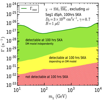
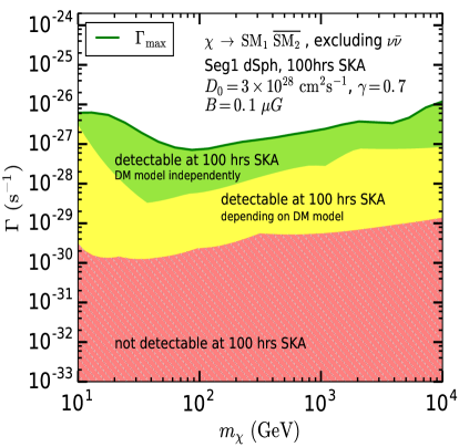
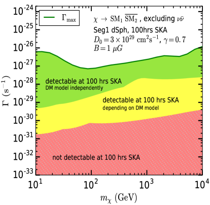
Figure 10: Top: Regions in the $m_{\chi}-\Gamma$ plane those are detectable in the 100 hours of observation of the Seg 1 dSph at the SKA are determined for Case 1, i.e., excluding DM decays to $\nu\bar{\nu}$ and varying the branching ratios of the remaining SM final states arbitrarily. Here we have considered $D_{0}=3\times 10^{28}{\rm cm}^{2}{\rm s}^{-1}$ and $B=1\mu{\rm G}$. $\Gamma_{\rm max}$ (the green solid line) is the upper limit on total $\Gamma$, obtained by combining the data of Planck CMB, Fermi-LAT IGRB and AMS-02 positron flux measurements. Bottom: The corresponding results for two other choices of the astrophysical parameters, viz., $D_{0}=3\times 10^{28}{\rm cm}^{2}{\rm s}^{-1}$, $B=0.1\mu{\rm G}$ (bottom left) and $D_{0}=3\times 10^{29}{\rm cm}^{2}{\rm s}^{-1}$, $B=1\mu{\rm G}$ (bottom right), which are even more conservative, are shown. The diffusion index $\gamma=0.7$ is assumed in all the cases. See the text for details.

In the top panel of Fig. 10, we have presented the SKA detectability of Case 1, i.e., DM decays to all possible SM final states other than $\nu\bar{\nu}$, assuming $D_{0}=3\times 10^{28}{\rm cm}^{2}{\rm s}^{-1}$, $\gamma=0.7$ and $B=1\mu{\rm G}$. The solid green line represents $\Gamma_{\rm max}$ obtained by analyzing the data of Planck CMB [4], Fermi-LAT IGRB [46] and AMS-02 cosmic-ray positron flux [53] observations (as discussed in Sec. 3.2). We find that, in this case, DM decays to two-body SM final states are branching ratio independently detectable at the SKA (100 hours) for $\Gamma{\;\raise 1.29167pt\hbox{$>$\kern-7.5pt\raise-4.73611pt\hbox{$\sim$}}\;}2\times 10^{-30}\,{\rm s}^{-1}$ when $m_{\chi}\sim 100\,{\rm GeV}$, and for decay widths greater than $2\times 10^{-29}\,{\rm s}^{-1}$ when $m_{\chi}\sim 1\,{\rm TeV}$. On the other hand, depending on the specific branching ratio combinations DM decays can be probed at the SKA for $\Gamma{\;\raise 1.29167pt\hbox{$>$\kern-7.5pt\raise-4.73611pt\hbox{$\sim$}}\;}7\times 10^{-32}\,{\rm s}^{-1}$ when $m_{\chi}\sim 100\,{\rm GeV}$, and for decay rates larger than $10^{-31}\,{\rm s}^{-1}$ for $m_{\chi}\sim 1\,{\rm TeV}$.

As an example, when $m_{\chi}\sim 100\,{\rm GeV}$, for an allowed value of $\Gamma\sim 10^{-31}\,{\rm s}^{-1}$, the radio fluxes coming from $\mu^{+}\mu^{-}$, $\tau^{+}\tau^{-}$, $q\bar{q}$, $b\bar{b}$ and $gg$ final states are above the SKA sensitivity level obtained assuming 100 hours of observation time. Therefore, for this parameter point DM decay induced radio signals are detectable if the DM decays to any one of the above-mentioned final states or any possible combination of them. On the other hand, for such a ($m_{\chi}$, $\Gamma$) point DM decay generated radio signals are non-detectable at the SKA when the decay occurs into $e^{+}e^{-}$, $\gamma\gamma$, $Z\gamma$ final states or any of their combinations. Therefore, this ($m_{\chi}$, $\Gamma$) point lies within the yellow region in Fig. 10 (top panel). However, if $\Gamma$ is increased at least by a factor of 20 the radio fluxes coming from the later mentioned decay modes also become detectable at the SKA. As a result, the resulting ($m_{\chi}$, $\Gamma$) point is detectable at the SKA for all possible branching ratio combinations and thus falls within the green region. On the contrary, if the decay rate is reduced by a factor of two, the resulting ($m_{\chi}$, $\Gamma$) point become non-detectable for all possible branching ratio combinations at the SKA and therefore, lies within the red-region .

On the other hand, if one considers $m_{\chi}\sim 1\,{\rm TeV}$, a point in the yellow region with $\Gamma\sim 2\times 10^{-31}\,{\rm s}^{-1}$ (allowed by the existing data), is detectable at the SKA if the DM decays into $q\bar{q}$, $b\bar{b}$, $t\bar{t}$, $gg$, $W^{+}W^{-}$, $ZZ$, $Zh$, $hh$ final states or any of their combinations. While the fluxes coming from $e^{+}e^{-}$, $\mu^{+}\mu^{-}$, $\tau^{+}\tau^{-}$, $\gamma\gamma$, $Z\gamma$ decay modes or any of their combinations are non-detectable at the SKA. If we increase the DM decay rate by two orders of magnitude, the resulting parameter point falls within the green region. While, if one reduces $\Gamma$ by a factor of two, the resulting ($m_{\chi}$, $\Gamma$) point lies within the red region. For $m_{\chi}\sim 100\,{\rm GeV}$ and $m_{\chi}\sim 1\,{\rm TeV}$ the detectability thresholds of the DM decay rate are $7\times 10^{-32}\,{\rm s}^{-1}$ and $10^{-31}\,{\rm s}^{-1}$, respectively, below which the radio fluxes are non-detectable for all possible branching ratio combinations at the 100 hours of the SKA observation. Hence, such parameter points fall inside the red region in Fig. 10 (top panel).

As mentioned earlier, apart from $D_{0}=3\times 10^{28}{\rm cm}^{2}{\rm s}^{-1}$ and $B=1\mu{\rm G}$, we have also considered other conservative values of these astrophysical parameters to demonstrate how our results depend on their variations. For example, in the bottom panel of Fig. 10 we have shown the regions of the DM parameter space, detectable or non-detectable in the 100 hours of observation at the SKA for Case 1, considering $D_{0}=3\times 10^{28}{\rm cm}^{2}{\rm s}^{-1}$, $B=0.1\mu{\rm G}$ (Fig. 10; bottom left) and $D_{0}=3\times 10^{29}{\rm cm}^{2}{\rm s}^{-1}$, $B=1\mu{\rm G}$ (Fig. 10; bottom right), respectively. The diffusion index $\gamma=0.7$ is assumed in both the cases.

Note that if one reduces $B$ the energy emission rate for synchrotron radiation decreases and consequently the produced radio signals will also be smaller (for details see [78]). This is manifested in the fact that for $m_{\chi}\sim 100\,{\rm GeV}$, DM decays are branching ratio independently detectable at the SKA for $\Gamma{\;\raise 1.29167pt\hbox{$>$\kern-7.5pt\raise-4.73611pt\hbox{$\sim$}}\;}6\times 10^{-29}\,{\rm s}^{-1}$, while DM decays can be probed at the SKA for certain specific combinations of branching fractions only if the decay rate is larger than $3\times 10^{-30}\,{\rm s}^{-1}$ (see Fig. 10; bottom left panel). Both of these values are more than one order of magnitude larger than the corresponding values obtained in the top panel of Fig. 10. For this DM mass, if the decay width goes below $3\times 10^{-30}\,{\rm s}^{-1}$, the corresponding parameter point falls within the red region.

On the other hand, as stated earlier, if one increases $D_{0}$ the DM decay induced electrons (positrons) escape from the diffusion zone of the considered dSph galaxy before radiating sufficient energies via synchrotron radiation and as a result, produced radio signals will also be suppressed (for details see [78]). This is evident from the bottom right panel of Fig. 10 where we have considered $D_{0}=3\times 10^{29}\,{\rm cm}^{2}{\rm s}^{-1}$, a value one order larger than the $D_{0}$ value assumed in the top panel of Fig. 10. In this case, decay of a 100 GeV DM particle is detectable, independent of the branching fractions of each DM decay mode, for $\Gamma{\;\raise 1.29167pt\hbox{$>$\kern-7.5pt\raise-4.73611pt\hbox{$\sim$}}\;}2\times 10^{-29}\,{\rm s}^{-1}$. For this $m_{\chi}$ value, DM decays are detectable for specific branching ratio combinations if the decay width is greater than $7\times 10^{-31}\,{\rm s}^{-1}$. The corresponding values of $\Gamma$ for $D_{0}=3\times 10^{28}\,{\rm cm}^{2}{\rm s}^{-1}$ were $2\times 10^{-30}\,{\rm s}^{-1}$ and $7\times 10^{-32}\,{\rm s}^{-1}$, respectively (see Fig. 10; top panel).

In principle, there can be further reduction (enhancement) of the detected flux in case one has higher (lower) $D_{0}$ and lower (higher) $B$. The effects of such reduction or enhancement in general can be surmised, for instance, from the detectability plots in the $B-D_{0}$ plane given in the Refs. [78, 81].

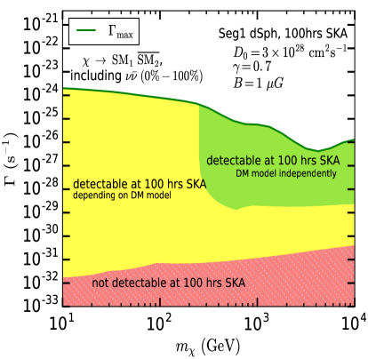
Figure 11: Classification of the DM parameter space (spanned by $m_{\chi}$ and $\Gamma$) based on the detectability at the SKA (for 100 hours of observation towards the Seg 1 dSph) is presented for Case 2, i.e., including DM decays to $\nu\bar{\nu}$ with arbitrary branching fractions. The choice for the astrophysical parameters made here are $D_{0}=3\times 10^{28}{\rm cm}^{2}{\rm s}^{-1}$, $\gamma=0.7$ and $B=1\,\mu{\rm G}$. $\Gamma_{\rm max}$ (the green solid line) is the upper limit obtained by using the data of Planck, Fermi-LAT, AMS-02 and Super-Kamiokande. See the text for details.

Fig. 11 shows the detectability of the decaying DM parameter space for Case 2 assuming 100 hours of observation time at the SKA. The results shown here are obtained for $D_{0}=3\times 10^{28}{\rm cm}^{2}{\rm s}^{-1}$, $\gamma=0.7$ and $B=1\mu{\rm G}$. In determining $\Gamma_{\rm max}$ (green solid line), we have used the data of Planck CMB [4], Fermi-LAT IGRB [46], AMS-02 positron flux [53] and Super-Kamiokande neutrino flux [59] observations.

For the $\nu\bar{\nu}$ final state, when $m_{\chi}$ is smaller than a few hundreds of GeV, final state $\nu\bar{\nu}$ pairs are of low energy and hence the resulting radio flux is also suppressed (see the discussions of Fig. 9; top right panel). As an example, for $m_{\chi}\sim 100\,{\rm GeV}$ and $\Gamma\sim 10^{-31}\,{\rm s}^{-1}$ (allowed by the existing data), $S_{\nu}$ for DM decays to $\mu^{+}\mu^{-}$, $\tau^{+}\tau^{-}$, $q\bar{q}$, $b\bar{b}$, $gg$ final states or any of their combinations are detectable at the SKA. On the other hand, radio fluxes for $e^{+}e^{-}$, $\gamma\gamma$, $Z\gamma$, $\nu\bar{\nu}$ final states or any of their combinations are non-detectable at the SKA. Therefore, this ($m_{\chi}$, $\Gamma$) point is detectable at the SKA for certain specific combinations of branching fractions. Keeping $m_{\chi}$ fixed, if we now increase $\Gamma$ to $\sim 10^{-25}\,{\rm s}^{-1}$, which is also allowed (see right panel of Fig. 7), DM decay induced radio signals are non-detectable at the SKA if DM decays dominantly into $\nu\bar{\nu}$ final state. Therefore, this parameter point, too, lies in the yellow region. In fact, for $m_{\chi}\lesssim 250\,{\rm GeV}$ and $\Gamma\gtrsim 10^{-29}-10^{-30}\,{\rm s}^{-1}$, DM decay generated radio flux is non-detectable at the SKA if $\nu\bar{\nu}$ is the dominant decay mode of the DM candidate. This implies that, detectability of any such parameter point depends on the branching fractions of each two-body SM final state (including $\nu\bar{\nu}$) which is manifested in the fact that the yellow region in Fig. 11 extends all the way up to $\Gamma_{\rm max}$ for $m_{\chi}{\;\raise 1.29167pt\hbox{$<$\kern-7.5pt\raise-4.73611pt\hbox{$\sim$}}\;}250\,{\rm GeV}$.

For higher values of $m_{\chi}$, $\nu\bar{\nu}$ pairs produced from DM decays are highly energetic and hence, the resulting radio flux is also detectable at the SKA (see the discussions of Fig. 9; bottom right panel). For example, when $m_{\chi}\sim 1\,{\rm TeV}$, the radio fluxes coming from the $\nu\bar{\nu}$ decay mode are detectable for $\Gamma\sim 10^{-29}\,{\rm s}^{-1}$, a value which is allowed by the existing observations. However, this point still lies in the yellow region, since the radio fluxes coming from the $e^{+}e^{-}$ final state are non-detectable at the SKA. One needs to increase $\Gamma$ nearly by a factor of two, so that the resulting ($m_{\chi}$, $\Gamma$) point becomes detectable for all possible decay modes. Therefore, when $m_{\chi}{\;\raise 1.29167pt\hbox{$>$\kern-7.5pt\raise-4.73611pt\hbox{$\sim$}}\;}250\,{\rm GeV}$, DM decays are detectable at the SKA for all possible branching ratio combinations of the two-body SM final states (including $\nu\bar{\nu}$) for $\Gamma{\;\raise 1.29167pt\hbox{$>$\kern-7.5pt\raise-4.73611pt\hbox{$\sim$}}\;}2\times 10^{-29}\,{\rm s}^{-1}$ (see Fig. 11). On the other hand, similar to top panel of Fig. 10, here, too, for $m_{\chi}\sim 100\,{\rm GeV}$, $\Gamma{\;\raise 1.29167pt\hbox{$<$\kern-7.5pt\raise-4.73611pt\hbox{$\sim$}}\;}7\times 10^{-32}\,{\rm s}^{-1}$ and for $m_{\chi}\sim 1\,{\rm TeV}$, any value of the DM decay width smaller than $10^{-31}\,{\rm s}^{-1}$ are non-detectable at the SKA.

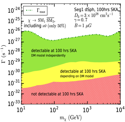
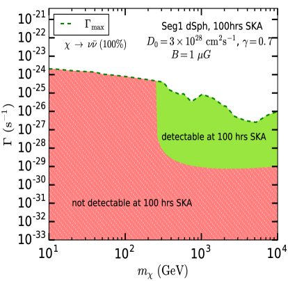
Figure 12: Left: SKA detectable regions (assuming 100 hours observation towards the Seg 1 dSph) in the $m_{\chi}-\Gamma$ plane and the maximum allowed decay width $\Gamma_{\rm max}$ (green dashed dotted line) are obtained assuming the $\nu\bar{\nu}$ final state to be produced with a branching ratio of $50\%$, i.e., Case 3. Right: Same as the left panel but for Case 4, i.e., considering exactly 100$\%$ branching ratio for the DM decay to the $\nu\bar{\nu}$ final state. The values of $D_{0}$, $\gamma$ and $B$ are same as the ones taken in Fig. 10; top panel and in Fig. 11. See the text for details.

From Fig. 11 it is clear that the inclusion of the $\nu\bar{\nu}$ decay mode in our analysis affects the detectability at the SKA considerably. This fact is further emphasized, in Fig. 12, where the results for Case 3 (left panel) and Case 4 (right panel) are presented assuming $D_{0}=3\times 10^{28}{\rm cm}^{2}{\rm s}^{-1}$, $\gamma=0.7$ and $B=1\mu{\rm G}$. In Case 3 (see Fig. 12; left panel), branching ratio for the $\nu\bar{\nu}$ final state being fixed at $50\%$, branching fractions of the remaining SM final states are varied in a way such that they add up to 0.5. The green dashed dotted line represents the $\Gamma_{\rm max}$ (as shown in Fig. 7; right panel). For $m_{\chi}{\;\raise 1.29167pt\hbox{$<$\kern-7.5pt\raise-4.73611pt\hbox{$\sim$}}\;}250\,{\rm GeV}$, $S_{\nu}$ coming from the $\nu\bar{\nu}$ final state is negligible and thus the radio fluxes are dominated by the contributions of the visible SM final states. As a result, throughout the considered mass range, DM decays are branching ratio independently detectable at the SKA for $\Gamma{\;\raise 1.29167pt\hbox{$>$\kern-7.5pt\raise-4.73611pt\hbox{$\sim$}}\;}10^{-30}-10^{-29}\,{\rm s}^{-1}$. On the other hand, the parameter point $m_{\chi}\sim 100\,{\rm GeV}$ and $\Gamma=2\times 10^{-31}\,{\rm s}^{-1}$ (allowed by Fig. 7; right panel) is detectable for DM decays to $\mu^{+}\mu^{-}$, $\tau^{+}\tau^{-}$, $q\bar{q}$, $b\bar{b}$, $gg$ final states or any of their combinations. However, such a ($m_{\chi}$, $\Gamma$) point is non-detectable for DM decays to any other channels. Thus, this parameter point lies in the yellow region. Note that here, the branching ratio of the $\nu\bar{\nu}$ final state being fixed at 50$\%$, the radio fluxes coming from the remaining SM final states are halved and the upper boundary of the red region has moved upward. As a result, now for $m_{\chi}\sim 100\,{\rm GeV}$, DM decay induced radio signals are non-detectable in the 100 hours of observation at the SKA for $\Gamma{\;\raise 1.29167pt\hbox{$<$\kern-7.5pt\raise-4.73611pt\hbox{$\sim$}}\;}10^{-31}\,{\rm s}^{-1}$, while, if $m_{\chi}\sim 1\,{\rm TeV}$, for any value of the decay width smaller than $3\times 10^{-31}\,{\rm s}^{-1}$, DM decay generated radio signals are not observable at the SKA. Contrary to Case 2 (shown in Fig. 11), here the green region is extended below $m_{\chi}\sim 250\,{\rm GeV}$ and the upper boundary of the red region has moved upward. Both of these are related to the fact that here we have fixed the branching ratio for the $\nu\bar{\nu}$ final state to be precisely $50\%$.

In the right panel of Fig. 12, detectability of Case 4 is shown for which the green dashed line represents $\Gamma_{\rm max}$. Here, DM decay width required for the detection of the $\nu\bar{\nu}$ channel dictates the boundary of the red and the green region, since now the DM decays entirely into $\nu\bar{\nu}$ with precisely $100\%$ branching ratio. Here, it is clear that for $m_{\chi}{\;\raise 1.29167pt\hbox{$<$\kern-7.5pt\raise-4.73611pt\hbox{$\sim$}}\;}250\,{\rm GeV}$ the radio signals originating from the $\nu\bar{\nu}$ final state are negligible enough to be detected at the SKA and hence for $m_{\chi}{\;\raise 1.29167pt\hbox{$<$\kern-7.5pt\raise-4.73611pt\hbox{$\sim$}}\;}250\,{\rm GeV}$, $\Gamma<\Gamma_{\rm max}$ is non-detectable. Clearly, the detectability in this case is quite different from that obtained in Case 2 (in Fig. 11) and Case 3 (Fig. 12; left panel).

In the end, we note that every parameter point in the yellow regions of Figs. 10 - 12 is detectable at the SKA (in 100 hours of observation) for certain combinations of branching fractions. Each such combination can be labelled as a separate DM model. On the other hand, following the analysis in Sec. 2.2, one finds constraints from existing astrophysical and cosmological data for each such ‘model’. This may lead to the exclusion of some model(s) corresponding to a particular point in the $m_{\chi}-\Gamma$ plane while other models are still allowed for those particular values of $m_{\chi}$ and $\Gamma$. Therefore, it remains meaningful to carry out radio observations in search of the latter class of models for any given ($m_{\chi}$, $\Gamma$) point in the yellow regions. For example, in Fig. 11, the point $m_{\chi}\simeq 40\,{\rm GeV}$, $\Gamma\simeq 2\times 10^{-28}\,{\rm s}^{-1}$ is ruled out by the existing data when the DM particle decays dominantly into $\gamma\gamma$ (see Fig. 3) or $e^{+}e^{-}$ (see Fig. 4) final states, while this parameter point is still allowed for DM decay to any other final state, say, $b\bar{b}$, $gg$, $\tau^{+}\tau^{-}$ etc. However, it is emphasized that radio signals corresponding to the allowed visible final states can be detectable in 100 hours of observation at the SKA for the given ($m_{\chi}$, $\Gamma$) point.

6 Summary and conclusions

In this work, we have performed a study of the indirect detection signals of a decaying scalar DM whose mass lies in the range 10 GeV - 10 TeV. We have investigated the implications of the existing observational data on the DM parameter space which set an upper limit for the allowed part of the DM parameter space. Then we explored the projected reach of the upcoming SKA radio telescope in discovering the DM decay induced radio signals coming from the Seg 1 dwarf galaxy. We start by presenting the limits on the DM decay width obtained from the data of Planck CMB [4], Fermi-LAT IGRB [46], AMS-02 positron flux [53] and Super-Kamiokande neutrino flux [59] observations assuming DM decays to any particular two-body SM final state with 100$\%$ branching ratio.

We have determined the maximum allowed decay width by varying the branching ratios of each individual SM final states arbitrarily in the range $0\%-100\%$, such that their sum always equals unity. In deriving this limit we have used the data of Planck CMB [4], Fermi-LAT IGRB [46] and AMS-02 positron observation [53] while considering DM decays to all possible SM final states other than neutrino-antineutrino pairs. We found that throughout our chosen range of the DM mass, decay rates smaller than $\sim 10^{-27}\,{\rm s}^{-1}$ are allowed. This limit is weaker by nearly an order of magnitude compared to the results obtained when 100$\%$ branching ratio is attributed to each individual DM decay mode. In addition, the Super-Kamiokande neutrino data of the Milky Way galaxy [59] are taken into account when DM decay to neutrino-antineutrino pairs is included in our analysis. For the $\nu\bar{\nu}$ final state the Super-Kamiokande constraints are found to be stronger than Planck, Fermi-LAT and AMS-02 limits particularly for DM particles lighter than $500\,{\rm GeV}$. On allowing the branching fractions of all SM final states, including that of the neutrino pairs, to vary in the range $0\%-100\%$, we found that for $m_{\chi}\sim\mathcal{O}({\rm TeV})$ or larger, the maximum value of the decay width that is allowed is $\sim 10^{-26}\,{\rm s}^{-1}$, while, for DM mass less than a hundred GeV, $\Gamma{\;\raise 1.29167pt\hbox{$<$\kern-7.5pt\raise-4.73611pt\hbox{$\sim$}}\;}10^{-24}\,{\rm s}^{-1}$ is consistent with the existing data. We have also studied the cases where the branching ratio for the neutrino-antineutrino final state is fixed at 50$\%$ and 100$\%$, respectively. When a branching fraction of $50\%$ is attributed to the $\nu\bar{\nu}$ final state the upper limit on the decay rate is found to be $\sim 10^{-27}\,{\rm s}^{-1}$ throughout the DM mass range considered, while for 100$\%$ branching to neutrino-antineutrino pairs, the maximum allowed decay width roughly follows the constraint obtained when an arbitrary branching fraction is allowed for the $\nu\bar{\nu}$ final state.

Next, we show how the DM parameter space that is allowed by the existing observations can be classified into regions which are detectable either for all possible branching ratio combinations or for certain specific combinations of branching fractions and non-detectable at the SKA, assuming 100 hours of observation towards the Seg 1 dSph. It is found that for DM decays to two-body SM final states (excluding $\nu\bar{\nu}$), decay rates greater than $10^{-31}\,{\rm s}^{-1}-10^{-29}\,{\rm s}^{-1}$ are detectable for all possible branching ratio combinations of the DM decay modes while $\Gamma{\;\raise 1.29167pt\hbox{$>$\kern-7.5pt\raise-4.73611pt\hbox{$\sim$}}\;}10^{-32}\,{\rm s}^{-1}-10^{-31}\,{\rm s}^{-1}$ are detectable only for certain specific branching ratio combinations, throughout the DM mass range 10 GeV - 10 TeV, assuming $D_{0}=3\times 10^{28}{\rm cm}^{2}{\rm s}^{-1}$ and $B=1\mu{\rm G}$. For even more conservative choices of these astrophysical parameters, namely, $D_{0}=3\times 10^{28}{\rm cm}^{2}{\rm s}^{-1},B=0.1\mu{\rm G}$ and $D_{0}=3\times 10^{29}{\rm cm}^{2}{\rm s}^{-1},B=1\mu{\rm G}$ we found that, the minimum values of the DM decay widths required for branching ratio independent detection at the SKA lie in the ranges $10^{-28}\,{\rm s}^{-1}-10^{-27}\,{\rm s}^{-1}$ and $10^{-29}\,{\rm s}^{-1}-10^{-28}\,{\rm s}^{-1}$, respectively.

On the other hand, when DM decay to neutrino-antineutrino pairs is included in our analysis and the corresponding branching fraction is also varied in the range $0\%-100\%$, we found that DM decays are detectable, independent of the branching ratio combinations, for decay widths larger than $\sim 10^{-29}\,{\rm s}^{-1}$, only if the DM particle is heavier than $250\,{\rm GeV}$, assuming $D_{0}=3\times 10^{28}{\rm cm}^{2}{\rm s}^{-1}$ and $B=1\mu{\rm G}$. For lower values of $m_{\chi}$ the detectability at the SKA depends on the branching fraction of the $\nu\bar{\nu}$ decay mode and if this is the dominant decay mode, DM decays are non-detectable at the SKA for all allowed values of the DM decay width. This fact is further explained by considering exactly 50$\%$ and 100$\%$ branching ratios for the neutrino-antineutrino final state. When the $\nu\bar{\nu}$ decay mode is produced with 50$\%$ branching ratio, one finds that, throughout the DM mass range under consideration, the DM decays are detectable for all branching ratio combinations of the non-neutrino SM final states only if the decay width is greater than $10^{-30}-10^{-29}\,{\rm s}^{-1}$. On the contrary, when 100$\%$ branching ratio is attributed to the neutrino final state the detectability at the SKA is entirely dictated by the radio fluxes coming from the $\nu\bar{\nu}$ channel and hence DM decays are detectable only for DM masses larger than $\sim 250\,{\rm GeV}$.

Note that the results presented here for the Seg 1 dSph would not change appreciably had one considered any other dSph such as Draco, Carina, Fornax etc. [133, 136, 151, 81, 77, 78], as the target. As pointed out in Sec. 2.1, the constraints on the DM decay rate obtained assuming DM decay is the only source of indirect detection signals will get even stronger in presence of appreciable DM annihilation rates, which would more severely constrain the fluxes coming from the DM decays. Additionally, note that the present analysis is applicable to, and consistent with, the scenarios discussed in Sec. 2.1 individually, so long as the decaying DM particle saturates the relic density. Although our basic methodology can be used, with appropriate modifications, to multi-component DM scenarios as well, where only some components are liable to decay. However, the constraints on the DM decay width tend to get weakened in such cases.

To sum it up, here we have considered a decaying scalar DM of mass in the 10 GeV - 10 TeV range. Taking all possible kinematically allowed two-body SM decay modes into account we have constrained the DM parameter space in a purely branching ratio independent fashion by utilizing the data of Planck CMB [4], Fermi-LAT IGRB [46], AMS-02 positron flux [53] and Super-Kamiokande neutrino flux [59] observations. The maximum allowed total DM decay width for each value of the DM mass has been derived by varying the branching ratios of all kinematically allowed DM decay modes arbitrarily so that their sum always equals unity. Any value of the DM decay rate larger than this maximum allowed value is ruled out by at least one existing observation for all possible branching ratio combinations. In the next step, the allowed region of the DM parameter space obtained this way has been classified into three distinct regions, viz., detectable for all possible branching ratio combinations, detectable for specific branching ratio combinations of the two-body SM final states and non-detectable, based on the detectability at the SKA assuming 100 hours of observation time towards the Segue 1 dSph. Our analysis shows that, irrespective of whether the DM candidate decays to neutrino-antineutrino pairs or not, the SKA can probe much deeper into the parameter space of a generic decaying scalar DM, as compared to the existing observations.

References

- [1] Y. Sofue and V. Rubin, Rotation curves of spiral galaxies, Ann. Rev. Astron. Astrophys. 39 (2001) 137–174, [astro-ph/0010594].
- [2] M. Markevitch, A. H. Gonzalez, L. David, A. Vikhlinin, S. Murray, W. Forman et al., A Textbook example of a bow shock in the merging galaxy cluster 1E0657-56, Astrophys. J. Lett. 567 (2002) L27, [astro-ph/0110468].
- [3] M. Markevitch, A. H. Gonzalez, D. Clowe, A. Vikhlinin, L. David, W. Forman et al., Direct constraints on the dark matter self-interaction cross-section from the merging galaxy cluster 1E0657-56, Astrophys. J. 606 (2004) 819–824, [astro-ph/0309303].
- [4] Planck collaboration, P. A. R. Ade et al., Planck 2015 results. XIII. Cosmological parameters, Astron. Astrophys. 594 (2016) A13, [1502.01589].
- [5] G. Jungman, M. Kamionkowski and K. Griest, Supersymmetric dark matter, Phys. Rept. 267 (1996) 195–373, [hep-ph/9506380].
- [6] G. Arcadi, M. Dutra, P. Ghosh, M. Lindner, Y. Mambrini, M. Pierre et al., The waning of the WIMP? A review of models, searches, and constraints, Eur. Phys. J. C 78 (2018) 203, [1703.07364].
- [7] L. Roszkowski, E. M. Sessolo and S. Trojanowski, WIMP dark matter candidates and searches—current status and future prospects, Rept. Prog. Phys. 81 (2018) 066201, [1707.06277].
- [8] L. J. Hall, K. Jedamzik, J. March-Russell and S. M. West, Freeze-In Production of FIMP Dark Matter, JHEP 03 (2010) 080, [0911.1120].
- [9] Y. Hochberg, E. Kuflik, T. Volansky and J. G. Wacker, Mechanism for Thermal Relic Dark Matter of Strongly Interacting Massive Particles, Phys. Rev. Lett. 113 (2014) 171301, [1402.5143].
- [10] E. Kuflik, M. Perelstein, N. R.-L. Lorier and Y.-D. Tsai, Elastically Decoupling Dark Matter, Phys. Rev. Lett. 116 (2016) 221302, [1512.04545].
- [11] G. Bélanger et al., LHC-friendly minimal freeze-in models, JHEP 02 (2019) 186, [1811.05478].
- [12] D. Choudhury, S. K. Gupta and B. Mukhopadhyaya, Right sneutrinos in a supergravity model and the signals of a stable stop at the Large Hadron Collider, Phys. Rev. D 78 (2008) 015023, [0804.3560].
- [13] S. K. Gupta, B. Mukhopadhyaya and S. K. Rai, Right-chiral sneutrinos and long-lived staus: Event characteristics at the large hadron collider, Phys. Rev. D 75 (2007) 075007, [hep-ph/0701063].
- [14] A. G. Hessler, A. Ibarra, E. Molinaro and S. Vogl, Probing the scotogenic FIMP at the LHC, JHEP 01 (2017) 100, [1611.09540].
- [15] N. Daci, I. De Bruyn, S. Lowette, M. H. G. Tytgat and B. Zaldivar, Simplified SIMPs and the LHC, JHEP 11 (2015) 108, [1503.05505].
- [16] E. Kuflik, M. Perelstein, N. R.-L. Lorier and Y.-D. Tsai, Phenomenology of ELDER Dark Matter, JHEP 08 (2017) 078, [1706.05381].
- [17] G. Elor, R. McGehee and A. Pierce, Maximizing Direct Detection with HYPER Dark Matter, 2112.03920.
- [18] F. Takayama and M. Yamaguchi, Gravitino dark matter without R-parity, Phys. Lett. B 485 (2000) 388–392, [hep-ph/0005214].
- [19] W. Buchmuller, L. Covi, K. Hamaguchi, A. Ibarra and T. Yanagida, Gravitino Dark Matter in R-Parity Breaking Vacua, JHEP 03 (2007) 037, [hep-ph/0702184].
- [20] A. Ibarra and D. Tran, Gamma Ray Spectrum from Gravitino Dark Matter Decay, Phys. Rev. Lett. 100 (2008) 061301, [0709.4593].
- [21] L. Covi and J. E. Kim, Axinos as Dark Matter Particles, New J. Phys. 11 (2009) 105003, [0902.0769].
- [22] M. Endo, K. Hamaguchi, S. P. Liew, K. Mukaida and K. Nakayama, Axino dark matter with R-parity violation and 130 GeV gamma-ray line, Phys. Lett. B 721 (2013) 111–117, [1301.7536].
- [23] A. Ghosh, A. Ibarra, T. Mondal and B. Mukhopadhyaya, Gamma-ray signals from multicomponent scalar dark matter decays, JCAP 01 (2020) 011, [1909.13292].
- [24] C. D. Carone and R. Primulando, A Froggatt-Nielsen Model for Leptophilic Scalar Dark Matter Decay, Phys. Rev. D 84 (2011) 035002, [1105.4635].
- [25] L. Feng and Z. Kang, Decaying Asymmetric Dark Matter Relaxes the AMS-Fermi Tension, JCAP 10 (2013) 008, [1304.7492].
- [26] B. Kyae and J.-C. Park, 130 GeV Fermi gamma-ray line from dark matter decay, Phys. Lett. B 718 (2013) 1425–1429, [1205.4151].
- [27] J.-C. Park and S. C. Park, Radiatively decaying scalar dark matter through U(1) mixings and the Fermi 130 GeV gamma-ray line, Phys. Lett. B 718 (2013) 1401–1406, [1207.4981].
- [28] Y. Mambrini, S. Profumo and F. S. Queiroz, Dark Matter and Global Symmetries, Phys. Lett. B 760 (2016) 807–815, [1508.06635].
- [29] S. Ando and K. Ishiwata, Constraints on decaying dark matter from the extragalactic gamma-ray background, JCAP 05 (2015) 024, [1502.02007].
- [30] K.-Y. Choi, B. Kyae and C. S. Shin, Decaying WIMP dark matter for AMS-02 cosmic positron excess, Phys. Rev. D 89 (2014) 055002, [1307.6568].
- [31] O. Catà, A. Ibarra and S. Ingenhütt, Dark matter decay through gravity portals, Phys. Rev. D 95 (2017) 035011, [1611.00725].
- [32] X. Sun, Gravity-Higgs portal for dark matter decay, 2112.04304.
- [33] W.-M. Yang, The Matter-Antimatter Asymmetry and Cold Dark Matter from The Left-Right Mirror Symmetric Model with The Global , 1309.1955.
- [34] W.-M. Yang, Baryogenesis and asymmetric dark matter from the left–right mirror symmetric model, Nucl. Phys. B 885 (2014) 505–523, [1405.0389].
- [35] G. Bhattacharyya, D. Das, P. B. Pal and M. N. Rebelo, Scalar sector properties of two-Higgs-doublet models with a global U(1) symmetry, JHEP 10 (2013) 081, [1308.4297].
- [36] T. Banks and N. Seiberg, Symmetries and Strings in Field Theory and Gravity, Phys. Rev. D 83 (2011) 084019, [1011.5120].
- [37] D. Harlow and H. Ooguri, Constraints on Symmetries from Holography, Phys. Rev. Lett. 122 (2019) 191601, [1810.05337].
- [38] A. Kusenko, M. Loewenstein and T. T. Yanagida, Moduli dark matter and the search for its decay line using Suzaku X-ray telescope, Phys. Rev. D 87 (2013) 043508, [1209.6403].
- [39] T. Hambye, D. Teresi and M. H. G. Tytgat, A Clockwork WIMP, JHEP 07 (2017) 047, [1612.06411].
- [40] S. Heeba, F. Kahlhoefer and P. Stöcker, Freeze-in production of decaying dark matter in five steps, JCAP 11 (2018) 048, [1809.04849].
- [41] E. Alcantara, L. A. Anchordoqui and J. F. Soriano, Hunting for superheavy dark matter with the highest-energy cosmic rays, Phys. Rev. D 99 (2019) 103016, [1903.05429].
- [42] T. R. Slatyer and C.-L. Wu, General Constraints on Dark Matter Decay from the Cosmic Microwave Background, Phys. Rev. D 95 (2017) 023010, [1610.06933].
- [43] C. E. Fichtel, G. A. Simpson and D. J. Thompson, Diffuse gamma radiation, Astrophys. J.; (United States) .
- [44] EGRET collaboration, P. Sreekumar et al., EGRET observations of the extragalactic gamma-ray emission, Astrophys. J. 494 (1998) 523–534, [astro-ph/9709257].
- [45] Fermi-LAT collaboration, A. A. Abdo et al., The Spectrum of the Isotropic Diffuse Gamma-Ray Emission Derived From First-Year Fermi Large Area Telescope Data, Phys. Rev. Lett. 104 (2010) 101101, [1002.3603].
- [46] Fermi-LAT collaboration, M. Ackermann et al., The spectrum of isotropic diffuse gamma-ray emission between 100 MeV and 820 GeV, Astrophys. J. 799 (2015) 86, [1410.3696].
- [47] W. Liu, X.-J. Bi, S.-J. Lin and P.-F. Yin, Constraints on dark matter annihilation and decay from the isotropic gamma-ray background, Chin. Phys. C 41 (2017) 045104, [1602.01012].
- [48] C. Blanco and D. Hooper, Constraints on Decaying Dark Matter from the Isotropic Gamma-Ray Background, JCAP 03 (2019) 019, [1811.05988].
- [49] C. Grimani et al., Measurements of the absolute energy spectra of cosmic-ray positrons and electrons above 7-GeV, Astron. Astrophys. 392 (2002) 287–294.
- [50] M. Schubnell, The Cosmic-Ray Positron and Electron Excess: An Experimentalist’s Point of View, in 44th Rencontres de Moriond on Very High Energy Phenomena in the Universe, pp. 271–274, 2009, 0905.0444.
- [51] AMS 01 collaboration, M. Aguilar et al., Cosmic-ray positron fraction measurement from 1 to 30-GeV with AMS-01, Phys. Lett. B 646 (2007) 145–154, [astro-ph/0703154].
- [52] PAMELA collaboration, O. Adriani et al., An anomalous positron abundance in cosmic rays with energies 1.5-100 GeV, Nature 458 (2009) 607–609, [0810.4995].
- [53] AMS collaboration, M. Aguilar et al., Electron and Positron Fluxes in Primary Cosmic Rays Measured with the Alpha Magnetic Spectrometer on the International Space Station, Phys. Rev. Lett. 113 (2014) 121102.
- [54] AMS collaboration, M. Aguilar et al., Precision Measurement of the Proton Flux in Primary Cosmic Rays from Rigidity 1 GV to 1.8 TV with the Alpha Magnetic Spectrometer on the International Space Station, Phys. Rev. Lett. 114 (2015) 171103.
- [55] AMS collaboration, M. Aguilar et al., Towards Understanding the Origin of Cosmic-Ray Positrons, Phys. Rev. Lett. 122 (2019) 041102.
- [56] A. Ibarra, A. S. Lamperstorfer and J. Silk, Dark matter annihilations and decays after the AMS-02 positron measurements, Phys. Rev. D 89 (2014) 063539, [1309.2570].
- [57] B.-Q. Lu and H.-S. Zong, Limits on dark matter from AMS-02 antiproton and positron fraction data, Phys. Rev. D 93 (2016) 103517, [1510.04032].
- [58] I. John and T. Linden, Cosmic-ray positrons strongly constrain leptophilic dark matter, JCAP 12 (2021) 007, [2107.10261].
- [59] Super-Kamiokande collaboration, K. Frankiewicz, Indirect searches for dark matter particles with the Super-Kamiokande detector, Nuovo Cim. C 38 (2016) 125.
- [60] R. Coy and T. Hambye, Neutrino lines from DM decay induced by high-scale seesaw interactions, JHEP 05 (2021) 101, [2012.05276].
- [61] T. Cohen, K. Murase, N. L. Rodd, B. R. Safdi and Y. Soreq, -ray Constraints on Decaying Dark Matter and Implications for IceCube, Phys. Rev. Lett. 119 (2017) 021102, [1612.05638].
- [62] IceCube collaboration, M. G. Aartsen et al., Search for neutrinos from decaying dark matter with IceCube, Eur. Phys. J. C 78 (2018) 831, [1804.03848].
- [63] IceCube collaboration, R. Abbasi et al., A Search for Neutrinos from Decaying Dark Matter in Galaxy Clusters and Galaxies with IceCube, PoS ICRC2021 (2021) 506, [2107.11527].
- [64] K. Ishiwata, O. Macias, S. Ando and M. Arimoto, Probing heavy dark matter decays with multi-messenger astrophysical data, JCAP 01 (2020) 003, [1907.11671].
- [65] M. Mateo, Dwarf galaxies of the Local Group, Ann. Rev. Astron. Astrophys. 36 (1998) 435–506, [astro-ph/9810070].
- [66] L. E. Strigari, S. M. Koushiappas, J. S. Bullock and M. Kaplinghat, Precise constraints on the dark matter content of Milky Way dwarf galaxies for gamma-ray experiments, Phys. Rev. D 75 (2007) 083526, [astro-ph/0611925].
- [67] L. E. Strigari, S. M. Koushiappas, J. S. Bullock, M. Kaplinghat, J. D. Simon, M. Geha et al., The Most Dark Matter Dominated Galaxies: Predicted Gamma-ray Signals from the Faintest Milky Way Dwarfs, Astrophys. J. 678 (2008) 614, [0709.1510].
- [68] L. E. Strigari, J. S. Bullock, M. Kaplinghat, J. D. Simon, M. Geha, B. Willman et al., A common mass scale for satellite galaxies of the Milky Way, Nature 454 (2008) 1096–1097, [0808.3772].
- [69] F. Acero et al., Constraints on the Galactic Population of TeV Pulsar Wind Nebulae Using Large Area Telescope Observations, Astrophys. J. 773 (2013) 77, [1306.5735].
- [70] A. Natarajan, J. B. Peterson, T. C. Voytek, K. Spekkens, B. Mason, J. Aguirre et al., Bounds on Dark Matter Properties from Radio Observations of Ursa Major II using the Green Bank Telescope, Phys. Rev. D 88 (2013) 083535, [1308.4979].
- [71] A. Natarajan, J. E. Aguirre, K. Spekkens and B. S. Mason, Green Bank Telescope Constraints on Dark Matter Annihilation in Segue I, 1507.03589.
- [72] M. Regis, L. Richter and S. Colafrancesco, Dark matter in the Reticulum II dSph: a radio search, JCAP 07 (2017) 025, [1703.09921].
- [73] M. Cirelli and M. Taoso, Updated galactic radio constraints on Dark Matter, JCAP 07 (2016) 041, [1604.06267].
- [74] M. Regis, S. Colafrancesco, S. Profumo, W. J. G. de Blok, M. Massardi and L. Richter, Local Group dSph radio survey with ATCA (III): Constraints on Particle Dark Matter, JCAP 10 (2014) 016, [1407.4948].
- [75] P. Bhattacharjee, D. Choudhury, K. Das, D. K. Ghosh and P. Majumdar, Gamma-ray and Synchrotron Radiation from Dark Matter annihilations in Ultra-faint Dwarf Galaxies, 2011.08917.
- [76] S. Colafrancesco, M. Regis, P. Marchegiani, G. Beck, R. Beck, H. Zechlin et al., Probing the nature of Dark Matter with the SKA, PoS AASKA14 (2015) 100, [1502.03738].
- [77] A. Kar, S. Mitra, B. Mukhopadhyaya and T. R. Choudhury, Can Square Kilometre Array phase 1 go much beyond the LHC in supersymmetry search?, Phys. Rev. D 99 (2019) 021302, [1808.05793].
- [78] A. Kar, S. Mitra, B. Mukhopadhyaya and T. R. Choudhury, Heavy dark matter particle annihilation in dwarf spheroidal galaxies: radio signals at the SKA telescope, Phys. Rev. D 101 (2020) 023015, [1905.11426].
- [79] B. Dutta, A. Kar and L. E. Strigari, Constraints on MeV dark matter and primordial black holes: Inverse Compton signals at the SKA, JCAP 03 (2021) 011, [2010.05977].
- [80] Z. Chen, Y.-L. S. Tsai and Q. Yuan, Sensitivity of SKA to dark matter induced radio emission, JCAP 09 (2021) 025, [2105.00776].
- [81] A. Ghosh, A. Kar and B. Mukhopadhyaya, Search for decaying heavy dark matter in an effective interaction framework: a comparison of -ray and radio observations, JCAP 09 (2020) 003, [2001.08235].
- [82] Braun, R. and others. https://astronomers.skatelescope.org/wp-content/uploads/2017/10/SKA-TEL-SKO-0000818-01_SKA1_Science_Perform.pdf, 2017.
- [83] M. Cirelli, E. Moulin, P. Panci, P. D. Serpico and A. Viana, Gamma ray constraints on Decaying Dark Matter, Phys. Rev. D 86 (2012) 083506, [1205.5283].
- [84] R. K. Leane, T. R. Slatyer, J. F. Beacom and K. C. Y. Ng, GeV-scale thermal WIMPs: Not even slightly ruled out, Phys. Rev. D 98 (2018) 023016, [1805.10305].
- [85] L. Covi, M. Grefe, A. Ibarra and D. Tran, Neutrino Signals from Dark Matter Decay, JCAP 04 (2010) 017, [0912.3521].
- [86] T. Sjostrand, S. Mrenna and P. Z. Skands, PYTHIA 6.4 Physics and Manual, JHEP 05 (2006) 026, [hep-ph/0603175].
- [87] C. Weniger, A Tentative Gamma-Ray Line from Dark Matter Annihilation at the Fermi Large Area Telescope, JCAP 08 (2012) 007, [1204.2797].
- [88] M. Su and D. P. Finkbeiner, Strong Evidence for Gamma-ray Line Emission from the Inner Galaxy, 1206.1616.
- [89] A. Arvanitaki, S. Dimopoulos, S. Dubovsky, P. W. Graham, R. Harnik and S. Rajendran, Astrophysical Probes of Unification, Phys. Rev. D 79 (2009) 105022, [0812.2075].
- [90] E. Nardi, F. Sannino and A. Strumia, Decaying Dark Matter can explain the e+- excesses, JCAP 01 (2009) 043, [0811.4153].
- [91] AMS Collaboration collaboration, M. Aguilar and et al., First result from the alpha magnetic spectrometer on the international space station: Precision measurement of the positron fraction in primary cosmic rays of 0.5–350 gev, Phys. Rev. Lett. 110 (Apr, 2013) 141102.
- [92] A. Ibarra, D. Tran and C. Weniger, Indirect Searches for Decaying Dark Matter, Int. J. Mod. Phys. A 28 (2013) 1330040, [1307.6434].
- [93] M. Garny, A. Ibarra, D. Tran and C. Weniger, Gamma-Ray Lines from Radiative Dark Matter Decay, JCAP 01 (2011) 032, [1011.3786].
- [94] M. Pierre, J. M. Siegal-Gaskins and P. Scott, Sensitivity of CTA to dark matter signals from the Galactic Center, JCAP 06 (2014) 024, [1401.7330].
- [95] A. Viana, H. Schoorlemmer, A. Albert, V. de Souza, J. P. Harding and J. Hinton, Searching for Dark Matter in the Galactic Halo with a Wide Field of View TeV Gamma-ray Observatory in the Southern Hemisphere, JCAP 12 (2019) 061, [1906.03353].
- [96] I. M. Oldengott, D. Boriero and D. J. Schwarz, Reionization and dark matter decay, JCAP 08 (2016) 054, [1605.03928].
- [97] Larger ACT collaboration, S. E. Boggs et al., The Advanced Compton Telescope Mission, New Astron. Rev. 50 (2006) 604–607, [astro-ph/0608532].
- [98] J. Greiner, K. Mannheim, F. Aharonian, M. Ajello, L. G. Balasz, G. Barbiellini et al., GRIPS - Gamma-Ray Imaging, Polarimetry and Spectroscopy, Experimental Astronomy 34 (Oct., 2012) 551–582, [1105.1265].
- [99] S. D. Hunter et al., A Pair Production Telescope for Medium-Energy Gamma-Ray Polarimetry, Astropart. Phys. 59 (2014) 18–28, [1311.2059].
- [100] G. Weidenspointner, M. Varendorff, K. Bennett, H. Bloemen, W. Hermsen, S. C. Kappadath et al., The Cdg Spectrum from 0.8-30 MeV Measured with COMPTEL Based on a Physical Model of the Instrumental Background, Astrophysical Letters and Communications 39 (Jan., 1999) 193.
- [101] A. W. Strong, I. V. Moskalenko and O. Reimer, Diffuse galactic continuum gamma rays. A Model compatible with EGRET data and cosmic-ray measurements, Astrophys. J. 613 (2004) 962–976, [astro-ph/0406254].
- [102] S. M. Krimigis, T. P. Armstrong, W. I. Axford, C. O. Bostrom, C. Y. Fan, G. Gloeckler et al., The low energy charged particle (lecp) experiment on the voyager spacecraft, Space Science Reviews 21 (Dec, 1977) 329–354.
- [103] S. E. C., C. A. C., M. F. B., H. B. C., L. N. and W. W. R., Voyager 1 observes low-energy galactic cosmic rays in a region depleted of heliospheric ions, Science 341 (Jul, 2013) 150–153.
- [104] K. K. Boddy and J. Kumar, Indirect Detection of Dark Matter Using MeV-Range Gamma-Ray Telescopes, Phys. Rev. D 92 (2015) 023533, [1504.04024].
- [105] M. Boudaud, J. Lavalle and P. Salati, Novel cosmic-ray electron and positron constraints on MeV dark matter particles, Phys. Rev. Lett. 119 (2017) 021103, [1612.07698].
- [106] e-ASTROGAM collaboration, M. Tavani et al., Science with e-ASTROGAM: A space mission for MeV–GeV gamma-ray astrophysics, JHEAp 19 (2018) 1–106, [1711.01265].
- [107] AMEGO collaboration, R. Caputo et al., All-sky Medium Energy Gamma-ray Observatory: Exploring the Extreme Multimessenger Universe, 1907.07558.
- [108] T. Aramaki, P. Hansson Adrian, G. Karagiorgi and H. Odaka, Dual MeV Gamma-Ray and Dark Matter Observatory - GRAMS Project, Astropart. Phys. 114 (2020) 107–114, [1901.03430].
- [109] D. Teresi, Clockwork Dark Matter, in 52nd Rencontres de Moriond on EW Interactions and Unified Theories, pp. 155–161, 2017, 1705.09698.
- [110] M. Cirelli, G. Corcella, A. Hektor, G. Hutsi, M. Kadastik, P. Panci et al., PPPC 4 DM ID: A Poor Particle Physicist Cookbook for Dark Matter Indirect Detection, JCAP 1103 (2011) 051, [1012.4515].
- [111] P. Ciafaloni, D. Comelli, A. Riotto, F. Sala, A. Strumia and A. Urbano, Weak Corrections are Relevant for Dark Matter Indirect Detection, JCAP 03 (2011) 019, [1009.0224].
- [112] www.marcocirelli.net/PPPC4DMID.html.
- [113] G. Bertone, W. Buchmuller, L. Covi and A. Ibarra, Gamma-Rays from Decaying Dark Matter, JCAP 11 (2007) 003, [0709.2299].
- [114] M. G. Baring, T. Ghosh, F. S. Queiroz and K. Sinha, New Limits on the Dark Matter Lifetime from Dwarf Spheroidal Galaxies using Fermi-LAT, Phys. Rev. D 93 (2016) 103009, [1510.00389].
- [115] J. Buch, M. Cirelli, G. Giesen and M. Taoso, PPPC 4 DM secondary: A Poor Particle Physicist Cookbook for secondary radiation from Dark Matter, JCAP 09 (2015) 037, [1505.01049].
- [116] A. W. Strong, I. V. Moskalenko and V. S. Ptuskin, Cosmic-ray propagation and interactions in the Galaxy, Ann. Rev. Nucl. Part. Sci. 57 (2007) 285–327, [astro-ph/0701517].
- [117] J. F. Navarro, C. S. Frenk and S. D. M. White, The Structure of cold dark matter halos, Astrophys. J. 462 (1996) 563–575, [astro-ph/9508025].
- [118] F. Iocco, M. Pato, G. Bertone and P. Jetzer, Dark matter distribution in the milky way: microlensing and dynamical constraints, Journal of Cosmology and Astroparticle Physics 2011 (nov, 2011) 029–029.
- [119] J. Bovy and S. Tremaine, On the local dark matter density, Astrophys. J. 756 (2012) 89, [1205.4033].
- [120] J. Lavalle, D. Maurin and A. Putze, Direct constraints on diffusion models from cosmic-ray positron data: Excluding the minimal model for dark matter searches, Phys. Rev. D 90 (2014) 081301, [1407.2540].
- [121] G. Giesen, M. Boudaud, Y. Génolini, V. Poulin, M. Cirelli, P. Salati et al., AMS-02 antiprotons, at last! Secondary astrophysical component and immediate implications for Dark Matter, JCAP 09 (2015) 023, [1504.04276].
- [122] C. Evoli, D. Gaggero and D. Grasso, Secondary antiprotons as a Galactic Dark Matter probe, JCAP 12 (2015) 039, [1504.05175].
- [123] L. Bergström, T. Bringmann, I. Cholis, D. Hooper and C. Weniger, New limits on dark matter annihilation from alpha magnetic spectrometer cosmic ray positron data, Phys. Rev. Lett. 111 (Oct, 2013) 171101.
- [124] A. W. Strong, E. Orlando and T. R. Jaffe, The interstellar cosmic-ray electron spectrum from synchrotron radiation and direct measurements, Astron. Astrophys. 534 (2011) A54, [1108.4822].
- [125] C. Evoli, D. Gaggero, D. Grasso and L. Maccione, Cosmic-Ray Nuclei, Antiprotons and Gamma-rays in the Galaxy: a New Diffusion Model, JCAP 10 (2008) 018, [0807.4730].
- [126] C. Evoli, D. Gaggero, A. Vittino, G. Di Bernardo, M. Di Mauro, A. Ligorini et al., Cosmic-ray propagation with : I. numerical solver and astrophysical ingredients, JCAP 02 (2017) 015, [1607.07886].
- [127] I. Cholis, D. Hooper and T. Linden, A Predictive Analytic Model for the Solar Modulation of Cosmic Rays, Phys. Rev. D 93 (2016) 043016, [1511.01507].
- [128] L. A. Cavasonza, H. Gast, M. Krämer, M. Pellen and S. Schael, Constraints on leptophilic dark matter from the AMS-02 experiment, Astrophys. J. 839 (2017) 36, [1612.06634].
- [129] Super-Kamiokande collaboration, K. Abe et al., Indirect search for dark matter from the Galactic Center and halo with the Super-Kamiokande detector, Phys. Rev. D 102 (2020) 072002, [2005.05109].
- [130] K. Frankiewicz, Indirect Search for Dark Matter with the Super-Kamiokande Detector, Ph.D. thesis, Warsaw, Inst. Nucl. Studies, 2018.
- [131] Fermi-LAT collaboration, M. Ackermann et al., Searching for Dark Matter Annihilation from Milky Way Dwarf Spheroidal Galaxies with Six Years of Fermi Large Area Telescope Data, Phys. Rev. Lett. 115 (2015) 231301, [1503.02641].
- [132] Fermi-LAT, DES collaboration, A. Albert et al., Searching for Dark Matter Annihilation in Recently Discovered Milky Way Satellites with Fermi-LAT, Astrophys. J. 834 (2017) 110, [1611.03184].
- [133] S. Colafrancesco, S. Profumo and P. Ullio, Detecting dark matter WIMPs in the Draco dwarf: A multi-wavelength perspective, Phys. Rev. D 75 (2007) 023513, [astro-ph/0607073].
- [134] G. Beck and S. Colafrancesco, A Multi-frequency analysis of dark matter annihilation interpretations of recent anti-particle and -ray excesses in cosmic structures, JCAP 05 (2016) 013, [1508.01386].
- [135] A. McDaniel, T. Jeltema, S. Profumo and E. Storm, Multiwavelength Analysis of Dark Matter Annihilation and RX-DMFIT, JCAP 09 (2017) 027, [1705.09384].
- [136] A. Kar, S. Mitra, B. Mukhopadhyaya, T. R. Choudhury and S. Tingay, Constraints on dark matter annihilation in dwarf spheroidal galaxies from low frequency radio observations, Phys. Rev. D 100 (2019) 043002, [1907.00979].
- [137] M. Geha, B. Willman, J. D. Simon, L. E. Strigari, E. N. Kirby, D. R. Law et al., The Least Luminous Galaxy: Spectroscopy of the Milky Way Satellite Segue 1, Astrophys. J. 692 (2009) 1464–1475, [0809.2781].
- [138] J. D. Simon, M. Geha, Q. E. Minor, G. D. Martinez, E. N. Kirby, J. S. Bullock et al., A COMPLETE SPECTROSCOPIC SURVEY OF THE MILKY WAY SATELLITE SEGUE 1: THE DARKEST GALAXY, The Astrophysical Journal 733 (may, 2011) 46.
- [139] S. Colafrancesco, S. Profumo and P. Ullio, Multi-frequency analysis of neutralino dark matter annihilations in the Coma cluster, Astron. Astrophys. 455 (2006) 21, [astro-ph/0507575].
- [140] E. Storm, T. E. Jeltema, M. Splettstoesser and S. Profumo, Synchrotron Emission from Dark Matter Annihilation: Predictions for Constraints from Non-detections of Galaxy Clusters with New Radio Surveys, Astrophys. J. 839 (2017) 33, [1607.01049].
- [141] E. Carretti, R. M. Crocker, L. Staveley-Smith, M. Haverkorn, C. Purcell, B. M. Gaensler et al., Giant Magnetized Outflows from the Centre of the Milky Way, Nature 493 (2013) 66, [1301.0512].
- [142] M. Regis, L. Richter, S. Colafrancesco, S. Profumo, W. J. G. de Blok and M. Massardi, Local Group dSph radio survey with ATCA – II. Non-thermal diffuse emission, Mon. Not. Roy. Astron. Soc. 448 (2015) 3747–3765, [1407.5482].
- [143] P. Rebusco, E. Churazov, H. Bohringer and W. Forman, Impact of stochastic gas motions on galaxy cluster abundance profiles, Mon. Not. Roy. Astron. Soc. 359 (2005) 1041–1048, [astro-ph/0501141].
- [144] P. Rebusco, E. Churazov, H. Boehringer and W. Forman, Effect of turbulent diffusion on iron abundance profiles, Mon. Not. Roy. Astron. Soc. 372 (2006) 1840–1850, [astro-ph/0608491].
- [145] T. E. Jeltema and S. Profumo, Searching for Dark Matter with X-ray Observations of Local Dwarf Galaxies, Astrophys. J. 686 (2008) 1045, [0805.1054].
- [146] J. Einasto, On the Construction of a Composite Model for the Galaxy and on the Determination of the System of Galactic Parameters, Trudy Astrofizicheskogo Instituta Alma-Ata 5 (1965) 87–100.
- [147] MAGIC collaboration, J. Aleksic et al., Searches for Dark Matter annihilation signatures in the Segue 1 satellite galaxy with the MAGIC-I telescope, JCAP 06 (2011) 035, [1103.0477].
- [148] R. Braun, T. L. Bourke, J. A. Green, E. Keane and J. Wagg, Advancing Astrophysics with the Square Kilometre Array, PoS AASKA14 (2015) 174.
- [149] C. Power, C. Lagos, B. Qin, C. Baugh, D. Cunnama, J. Fu et al., Galaxy Formation & Dark Matter Modelling in the Era of the Square Kilometre Array, PoS AASKA14 (2015) 133.
- [150] R. Ghara, T. R. Choudhury and K. K. Datta, 21-cm signature of the first sources in the Universe: Prospects of detection with SKA, Mon. Not. Roy. Astron. Soc. 460 (2016) 827–843, [1511.07448].
- [151] A. Geringer-Sameth, S. M. Koushiappas and M. Walker, Dwarf galaxy annihilation and decay emission profiles for dark matter experiments, Astrophys. J. 801 (2015) 74, [1408.0002].