Phantoms and strange attractors in cosmology

Jorge G. Russo

Institució Catalana de Recerca i Estudis Avançats (ICREA),

Pg. Lluis Companys, 23, 08010 Barcelona, Spain.

Departament de Física Cuántica i Astrofísica and Institut de Ciències del Cosmos,

Universitat de Barcelona, Martí Franquès, 1, 08028 Barcelona, Spain.

E-Mail: jorge.russo@icrea.cat

ABSTRACT

We study a cosmological model of gravity coupled to three, self-interacting scalar fields, one of them with negative kinetic term. The theory has cosmological solutions described by three-dimensional quadratic autonomous equations. Remarkably, the dynamical system has strange attractors, which are in fact very similar to the classic Lorenz attractor. The associated chaotic cosmologies exhibit highly fluctuating periods of contraction and expansion, alternating with long, steady periods in a de Sitter-like phase.

1 Introduction

Chaos in cosmology arises naturally and has been widely discussed in many different contexts and models [1, 2]. A plausible reason behind the chaos is the influence of arbitrary perturbations that become uncontrollable near the cosmological singularity, giving rise to complicated, non-homogeneous geometries. These can initially be described by generalized Kasner metrics, but soon acquire a strong oscillatory behavior that becomes stochastic [2]. The classical description fails as physics enters the unknown quantum realm of gravity.

Historically, chaos appeared in a simplified model of atmospheric convection proposed by the mathematician and meteorologist Edward Lorenz in 1963. The model gave rise to a three-dimensional quadratic autonomous system, whose detailed analysis led to the discovery of strange attractors. The cosmological model studied here is closely related to the Lorenz model.

Here the analysis of chaos will be greatly simplified because we will be working with first-order equations. The idea is to construct cosmological models for multiscalar fields interacting with gravity, where the scalar potential can be derived from a (fake) superpotential. This plays the role of a Hamilton’s characteristic function of Hamilton-Jacobi theory. The method is standard (a discussion can be found in [3]). Starting with a Lagrangian

$$L=\frac{1}{2}G_{ij}\partial_{t}\phi^{i}\partial_{t}\phi^{j}-V(\phi^{i})\ ,$$ (1)

one assumes that a superpotential $W$ exists, satisfying

$$V=-\frac{1}{2}G^{ij}\frac{\partial W}{\partial\phi^{i}}\frac{\partial W}{\partial\phi^{j}}\ .$$ (2)

Then, the solutions of the first order system

$$\partial_{t}\phi^{i}=\epsilon G^{ij}\frac{\partial W}{\partial\phi^{j}}\ ,$$ (3)

with $\epsilon=\pm 1$, solve the second-order equations. In general, there may be solutions of the second-order equations that are not described by the first-order system, but our aim here is to discuss specific solutions.

Cosmological models described in terms of trajectories in a three dimensional space have first appeared in [4], in the context of the “universal” one-axion model (generalizing the model of [5] where cosmologies were associated to trajectories in a 2d space). In the case of [4], too, the dynamics is governed by first-order equations, although this reduction to a first-order system occurs in a completely different way (for other approaches, see e.g. [6]). The three-dimensional autonomous system of [4] is never chaotic in any range of the parameters. An important property of the axion-two dilaton system of [4] is that, for specific values of the parameters, represents a consistent truncation of massive maximal supergravities. While the scalar field potential for the present models is motivated by closely related potentials appearing in D-brane lagrangians, it differs from these in an essential way.

2 The non-chaotic D-brane model

The scalar field potential that we will choose for our cosmological model is motivated by a closely related potential that appears in some supersymmetric Yang-Mills theories. Cosmological models based on similar potentials with matrix-valued scalar fields have been investigated in the past [7]. More recently, there has also been interest in chaos in matrix models and Yang-Mills theories, motivated by the holographic description of black hole horizons and the onset of thermalization (see e.g. [8, 9, 10, 11]).

Here we shall consider the ${\cal N}=1^{*}$ theory that arises by adding mass terms to the three chiral multiplets $\hat{\Phi}_{i}$, $i=1,2,3$, of the ${\cal N}=4$ $SU(N)$ super Yang-Mills theory. It has a superpotential

$$W_{{\cal N}=1}={\rm Tr}\left([\hat{\Phi}_{1},[\hat{\Phi}_{2},\hat{\Phi}_{2}]]+m_{1}\hat{\Phi}_{1}^{2}+m_{2}\hat{\Phi}_{2}^{2}+m_{3}\hat{\Phi}_{3}^{2}\right)\ .$$ (4)

The $\hat{\Phi}_{123}$ are in the adjoint representation of $SU(N)$. Let us denote by $\varphi_{i}$, $i=1,...,6$ the six (real) scalar components. The bosonic part of the Lagrangian containing the scalar fields is

$$L={\rm Tr}\left(-\frac{1}{2}D_{\mu}\varphi_{i}D^{\mu}\varphi_{i}-\frac{1}{2}m_{i}^{2}\varphi_{i}\varphi_{i}+\frac{1}{4}[\varphi_{i},\varphi_{j}][\varphi_{i},\varphi_{j}]\right)\ .$$ (5)

We shall consider the ansatz

$$Z_{1}\equiv\varphi_{1}+i\varphi_{4}=x(\sigma)e^{-i\mu_{1}t}\alpha_{1}\ ,$$

$$Z_{2}\equiv\varphi_{2}+i\varphi_{5}=y(\sigma)e^{-i\mu_{2}t}\alpha_{2}\ ,$$

$$Z_{3}\equiv\varphi_{3}+i\varphi_{6}=z(\sigma)e^{-i\mu_{3}t}\alpha_{3}\ ,$$ (6)

where $\sigma$ is one of the spatial coordinates and $\alpha_{123}$ are any $N\times N$ representation of the $SU(2)$ algebra,

$$\big{[}\alpha_{i},\alpha_{j}\big{]}=2i\epsilon_{ijk}\alpha_{k}\ ,\qquad{\rm Tr}[\alpha_{i}\cdot\alpha_{j}]=a_{N}\,\delta_{ij}\ .$$ (7)

For irreducible representations, $a_{N}=\frac{1}{3}N(N^{2}-1)$; for reducible representations, the coefficient analog to $a_{N}$ is smaller. We assume a configuration where the gauge field vanishes. Note that the Gauss law constraint

$$\sum_{i}\left[\partial_{\mu}\varphi_{i},\varphi_{i}\right]=0\ ,$$ (8)

is identically satisfied by the given ansatz.

The resulting equations for $x$, $y$, $z$ can be derived from the effective Lagrangian

$$L_{\rm eff}=-\frac{1}{2}\Big{(}(\partial_{\sigma}x)^{2}+(\partial_{\sigma}y)^{2}+(\partial_{\sigma}z)^{2}+M_{1}^{2}x^{2}+M_{2}^{2}y^{2}+M_{3}^{2}z^{2}\Big{)}-2\big{(}x^{2}y^{2}+x^{2}z^{2}+y^{2}z^{2}\big{)},$$ (9)

where

$$\quad M_{i}=\pm\sqrt{-\mu_{i}^{2}+m_{i}^{2}}\ .$$ (10)

The second-order equations for $x(\sigma),\ y(\sigma),\ z(\sigma)$ are, in general, difficult to solve, but, when $M_{1}+M_{2}+M_{3}=0$, one can write first-order equations using the following superpotential

$$W=\frac{1}{2}(M_{1}x^{2}+M_{2}y^{2}+M_{3}z^{2})+2xyz\ .$$ (11)

It satisfies

$$V=\frac{1}{2}(\partial_{x}W\partial_{x}W+\partial_{y}W\partial_{y}W+\partial_{z}W\partial_{z}W)\ ,$$ (12)

where

$$V\equiv\frac{1}{2}(M_{1}^{2}x^{2}+M_{2}^{2}y^{2}+M_{3}^{2}z^{2})+2(x^{2}y^{2}+x^{2}z^{2}+y^{2}z^{2})\ ,$$

provided

$$M_{1}+M_{2}+M_{3}=0\ .$$ (13)

The associated first-order equations (3) are, therefore,

$$x^{\prime}=M_{1}x+2yz\ ,\quad y^{\prime}=M_{2}y+2xz\ ,\quad z^{\prime}=M_{3}z+2xy\ .$$ (14)

3 Chaos with ghosts

While the dynamical system (14) is not chaotic, it is nevertheless closely related to a chaotic system discovered in [12, 13], by looking for generalizations of the classic Lorenz chaotic system. The equations are

$$x^{\prime}=ax+yz\ ,\quad y^{\prime}=by+xz\ ,\quad z^{\prime}=cz-xy\ .$$ (15)

The difference with (14) lies in the opposite sign in the quadratic term of the $z$ equation, and it turns out to be a crucial difference (the extra factor of 2 in the quadratic terms in (14) is not important as it can be rescaled away). As discussed below, another important difference is that, in (15), $a+b+c$ is required to be negative, which ensures that the volume in phase space contracts under the time evolution, as expected for a strange attractor.

Equations equivalent to (15) can be derived from a field theory Lagrangian if one reverses the sign in the kinetic term of the $z$ particle, viz. one is to consider a model containing three scalar fields $(X,Y,Z)$ with the following Lagrangian

$$L = -\frac{1}{2}G_{ij}g^{\mu\nu}\partial_{\mu}X^{i}\partial_{\nu}X^{j}-V$$ (16)

$$= \frac{1}{2}g^{\mu\nu}\left(\partial_{\mu}Z\partial_{\nu}Z-\partial_{\mu}X\partial_{\nu}X-\partial_{\mu}Y\partial_{\nu}Y\right)-V\ ,$$

where $g_{\mu\nu}={\rm diag}(-1,1,...,1)$, $X^{i}=(X,Y,Z)$, $i=1,2,3$, with a target metric $G_{ij}={\rm diag}(1,1,-1)$. The potential of the model is defined as follows:

$$V=\frac{1}{2}(cZ-XY)^{2}-\frac{1}{2}(aX+YZ)^{2}-\frac{1}{2}(bY+XZ)^{2}\ .$$ (17)

Now consider solutions that have only time dependence. The Lagrangian becomes

$$L=\frac{1}{2}\left(-\dot{Z}^{2}+\dot{X}^{2}+\dot{Y}^{2}\right)-V\ .$$ (18)

The potential (17) can be derived from the superpotential

$$W=\frac{1}{2}\left(aX^{2}+bY^{2}-cZ^{2}\right)+XYZ\ .$$ (19)

It satisfies the relation (2),

$$V=-\frac{1}{2}G^{ij}\partial_{i}W\partial_{j}W=\frac{1}{2}(cZ-XY)^{2}-\frac{1}{2}(aX+YZ)^{2}-\frac{1}{2}(bY+XZ)^{2}\ ,$$ (20)

Using the general formulas (3), we find the following first-order equations,

$$\dot{X}=aX+YZ\ ,\qquad\dot{Y}=bY+XZ\ ,\qquad\dot{Z}=cZ-XY\ ,$$ (21)

which are identical to (15). Here we have taken $\epsilon=1$; the opposite sign choice corresponds to the time-reversed solutions.

Thus there is a family of time-dependent solutions in the field theory that are governed by the system (15). This system is chaotic in a large range of parameters. The basic dynamical properties of this chaotic system, including bifurcations, symmetries, periodic windows and Lyapunov exponents are investigated in detail in [13], so this analysis will not be reproduced here. However, it is worth noting the important differences from the dynamical system (14), which can be understood analytically. Consider a closed surface in phase space of volume ${\cal V}$. The time derivative is given by

$$\frac{\dot{\cal V}}{\cal V}=\vec{\nabla}\cdot\dot{\vec{X}}=a+b+c\ ,\qquad\vec{X}=(X,Y,Z)\ .$$

When $a+b+c<0$, the volume in phase space shrinks; the system is dissipative. Just like in the Lorenz attractor, the volume in phase space decays exponentially, showing the existence of an attracting set of zero volume. In the system (14), one has $\dot{\cal V}=0$ by virtue of the identity $M_{1}+M_{2}+M_{3}=0$. This is already a sign that the system (14) is not chaotic.

Choosing $a<0,b<0$ and $c>0$, the system (21) has five fixed points, one at the origin $(X,Y,Z)=(0,0,0)$, and other four fixed points located at

$$(X_{0},Y_{0},Z_{0})\ ,\quad(X_{0},-Y_{0},-Z_{0})\ ,\quad(-X_{0},Y_{0},-Z_{0})\ ,\quad(-X_{0},-Y_{0},Z_{0})\ .$$ (22)

where $X_{0}=\sqrt{-bc},\ Y_{0}=\sqrt{-ac},\ Z_{0}=\sqrt{ab}$. If a fixed point is fully attractive in all directions, some trajectories will not be chaotic as they will fall into the attractive fixed point. Chaos is favored when all fixed points have repulsive directions. The fixed point at the origin has a repulsive direction since one of the eigenvalues is positive, $c>0$. Linearization around the other four fixed points give eigenvalues corresponding to the three roots of the cubic equation

$$\lambda^{3}-(a+b+c)\lambda^{2}+4abc=0\ .$$ (23)

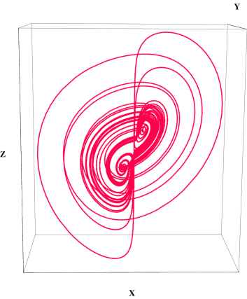
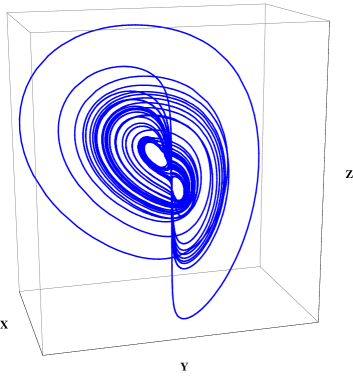
(a)	(b)

Figure 1: The double-scroll strange attractor for two different sets of parameters (a) $a=-10$, $b=-4$, $c=20/7$. (b) $a=-2$, $b=-4$, $c=4/3$.

With the choice of signs for $a,b,c$, with $a+b+c<0$, one eigenvalue is real and negative; the other two eigenvalues are complex conjugates. Taking $a,b<0$ and $c>0$, the complex eigenvalues have a positive real part, so they give rise to repulsive directions. A strange attractor then appears, as illustrated in figures 1a,b.

4 Cosmological model

4.1 Cosmological models with first-order equations

Consider the following Lagrangian describing Einstein gravity coupled to $n$ scalar fields $\phi^{I}$ with self-interactions,

$$L=\frac{1}{2}\sqrt{-{\rm det}g}\left(2R-g^{\mu\nu}G_{IJ}(\phi)\partial_{\mu}\phi^{I}\partial_{\nu}\phi^{J}-2V(\phi)\right)\ .$$ (24)

We shall study flat FLRW cosmologies of the form

$$ds^{2}=-e^{2\alpha\varphi}f^{2}d\tau^{2}+e^{2\beta\varphi}\left(dx_{1}^{2}+...+dx_{d-1}^{2}\right)\ ,$$ (25)

with $\varphi=\varphi(\tau)$, $f=f(\tau)$, $\phi^{I}=\phi^{I}(\tau)$, and

$$\alpha=(d-1)\beta\ ,\qquad\beta=\frac{1}{\sqrt{2(d-1)(d-2)}}\ .$$ (26)

The Einstein equations and the scalar field equations of the original Lagrangian then reduce to the Euler-Lagrange equations of the effective Lagrangian

$$L_{\rm eff}=\frac{1}{2f}\left(-\dot{\varphi}^{2}+G_{IJ}(\phi){\dot{\phi}^{I}}{\dot{\phi}^{J}}\right)-fe^{2\alpha\varphi}V(\phi)\ .$$ (27)

Even for very simple potentials, solving the system of coupled second-order differential equations is very complicated. Here we will be using a simple construction where equations reduce to more tractable first-order differential equations. The idea is to identify a class of potentials that can be derived from a superpotential. We define the following superpotential:

$${\cal W}=e^{\alpha\varphi}F(\phi)\ .$$ (28)

Then we choose the potential

$$2e^{2\alpha\varphi}\,V\equiv(\partial_{\varphi}{\cal W})^{2}-G^{IJ}\partial_{I}{\cal W}\partial_{J}{\cal W}=e^{2\alpha\varphi}\left(\alpha^{2}F^{2}-G^{IJ}\partial_{I}F\partial_{J}F\right)\ .$$ (29)

Note that the potential in general is not bounded from below. This is a common feature in models arising from truncation of (gauged) supergravity/string theory (the simplest example being a negative cosmological constant).

With the choice (29) for the scalar potential, a family of cosmological solutions can be found by studying the following first-order system:

$$\dot{\varphi}=-f\partial_{\varphi}{\cal W}=-\alpha fe^{\alpha\varphi}F,\qquad\dot{\phi_{I}}=fG^{IJ}\partial_{J}{\cal W}=fe^{\alpha\varphi}G^{IJ}\partial_{J}F\ .$$ (30)

Choosing $f=e^{-\alpha\phi}$, the factor $e^{\alpha\varphi}$ cancels out and the first-order system takes the simple form

$$\dot{\varphi}=-\alpha F(\phi),\qquad\dot{\phi_{I}}=G^{IJ}\partial_{J}F(\phi)\ .$$ (31)

Note that an alternate choice of time, corresponding to taking $f=e^{-\alpha\phi}/F$, identifies the time coordinate with $-\varphi/\alpha$. However, for our purposes it is more convenient to choose $f=e^{-\alpha\phi}$. Then, the standard FLRW cosmological time $t$, defined by $dt=e^{\alpha\varphi}fd\tau$, coincides with $\tau$.

4.2 The chaotic cosmological model

Let us now apply this construction to the three-scalar-field model studied in the previous section, coupled to gravity. The lagrangian is

$$L=\frac{1}{2}\sqrt{-{\rm det}g}\left(2R-G_{ij}g^{\mu\nu}\partial_{\mu}X^{i}\partial_{\nu}X^{j}-2V\right)\ ,$$ (32)

where $G_{ij}={\rm diag}(1,1,-1)$ as in (16) and the potential will be specified shortly. The model contains a ghost field. Cosmological models with ghosts have been extensively used in cosmology to account for phantom phases where the equation of state parameter $w$ is less than $-1$ (see e.g. [14, 15] and references therein). As usual, the presence of a ghost leads to well-known problems in the quantum theory, related to unitarity or vacuum stability (a discussion on phenomenological bounds can be found in [16]). In this work, of course, our goal is not the quantum consistency of the model, but rather the understanding of the conditions under which classical deterministic chaos, such as that of generalized Lorenz models, can be incorporated into field theory.

We now consider the cosmological FLRW ansatz (25). The remaining Einstein’s equations and scalar field equations can be derived from the effective Lagrangian

$$L_{\rm eff}=\frac{1}{2f}\left(-\dot{\varphi}^{2}-\dot{Z}^{2}+\dot{X}^{2}+\dot{Y}^{2}\right)-fe^{2\alpha\varphi}V\ .$$ (33)

The $f$ equation gives rise to the constraint:

$$\dot{\varphi}^{2}+\dot{Z}^{2}-\dot{X}^{2}-\dot{Y}^{2}=2f^{2}e^{2\alpha\varphi}V\ .$$ (34)

We shall choose the standard cosmological time, corresponding to the choice $f=e^{-\alpha\phi}$. We now consider a superpotential of the form

$${\cal W}=e^{\alpha\varphi}\,W\ ,$$ (35)

where $W$ given by (19). The potential is then defined by

$$2V = \alpha^{2}W^{2}+(\partial_{Z}W)^{2}-(\partial_{X}W)^{2}-(\partial_{Y}W)^{2}$$ (36)

$$= \frac{\alpha^{2}}{4}\left(aX^{2}+bY^{2}-cZ^{2}+2XYZ\right)^{2}$$

$$+ (cZ-XY)^{2}-(aX+YZ)^{2}-(bY+ZX)^{2}\ .$$

The parameters $a,b,c$ represent self-interaction couplings for the three scalar fields. Remarkably, with the choice $f=e^{-\alpha\varphi}$, we find exactly the first-order system (21), supplemented with the additional equation

$$\dot{\varphi}=-\alpha W\ .$$ (37)

The solutions to these equations solve the second-order equations of the original theory (32) and the constraint (34). One can first solve (21) for $X,Y,Z$ and then substitute the solution into $W$, see (19). The cosmological metric is then obtained by integrating (37).

Thus trajectories in the three-dimensional space $(X,Y,Z)$ are governed by the same autonomous system (21) as in the generalized Lorenz system studied by [13]. Chaotic trajectories appear for a wide range of couplings. For example, the choice

$$a=-10\ ,\qquad b=-4\ ,\qquad c=-\frac{ab}{a+b}\ ,$$

studied in [13], gives rise to a double-scroll strange attractor with a spectrum of Lyapunov exponents [13] $\lambda_{1}\approx 1,17$, $\lambda_{2}=0$ and $\lambda_{3}\approx-12.3$ and Lyapunov dimension $d_{L}\approx 2.1$ for initial value $(1,1,1)$ (other choices of $c$ can generate a 4-scroll chaotic attractor). Note that the motion is bounded, despite the potential having unstable directions at infinity.

There is a range of parameters $a,b,c$ where there are no chaotic trajectories. For example, when $a+b+c>0$, trajectories typically go to infinity. On the other hand, when $a,b,c$ are all negative, the fixed point at the origin is attractive and solutions can approach at a scaling solution at this attractive fixed point. These alternative regimes give rise to more familiar cosmologies. However, our main focus here is to investigate the properties of the cosmological solutions associated with the chaotic trajectories, since this appears to be a new behavior, which, to our knowledge, has not been considered before.

The scale factor is $a=e^{\beta\varphi}$. The universe expands if $\dot{a}=\beta e^{\beta\varphi}\dot{\varphi}>0$. Since $\dot{\varphi}=-\alpha W$, periods of expansion occurs when the trajectories go through a region where $W<0$. Along the chaotic trajectories, $W$ fluctuates taking positive and negative values. This is shown in fig. 2a. Thus the universe undergoes periods of contraction and expansion. Surprisingly, the cosmological evolution also shows periods with steady behavior. Let us now discuss this feature in more detail.

The expansion is accelerated when $\ddot{a}>0$. From the relation

$$R_{00}=-(d-1)\frac{\ddot{a}}{a}\ ,$$ (38)

one sees that universe undergoes an accelerated expansion in the regions where $W<0$ and $R_{00}<0$. From the Einstein’s equations, we find

$$R_{00}=\frac{1}{2}\left(\dot{X}^{2}+\dot{Y}^{2}-\dot{Z}^{2}-\frac{2}{d-2}V\right)\ .$$ (39)

Upon using the constraint, this reduces to

$$R_{00}=\frac{1}{2}\left(\dot{\varphi}^{2}-\frac{2(d-1)}{d-2}V\right)=\frac{d-1}{4(d-2)}\left(W^{2}-4V\right)\ .$$ (40)

where $\dot{\varphi}=-\alpha W$ has been used.

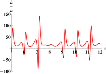
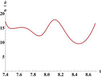
(a)	(b)

Figure 2: (a) The expansion velocity given by the Hubble parameter $H(t)=\dot{a}(t)/a(t)$ for a solution in the $d=4$ theory with couplings $a=-10$, $b=-4$, $c=20/7$. The cosmological evolution shows periods of rapid expansion and contraction, alternating with steady periods where $w\approx-1$. (b) Same plot enlarged, showing in detail a period of accelerated expansion where $w\approx-1$ (cf. fig. 3).

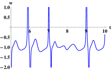
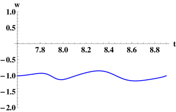
(a)	(b)

Figure 3: (a) $w$ as a function of time for the same trajectory as in fig. 2. The expansion is accelerated in the region $w<-1/3$, and it approaches a de Sitter-like expansion when $w\approx-1$. There are singular points where $W$ vanishes, corresponding to $\dot{a}=0$. (b) Same plot enlarged in a region where $w\approx-1$.

Following [4], we can study the evolution of the equation of state along a given trajectory. The equation of state is given by $p=w\rho$, where $p$ is the matter pressure and $\rho$ is the energy density. Their explicit expression is found by computing $T_{00}=-g_{00}\rho\ ,\ \ T_{ij}=g_{ij}p\$. For the present model,

$$\rho=\frac{1}{4}\left(\dot{X}^{2}+\dot{Y}^{2}-\dot{Z}^{2}+2V\right)\ ,\qquad p=\frac{1}{4}\left(\dot{X}^{2}+\dot{Y}^{2}-\dot{Z}^{2}-2V\right)\ .$$ (41)

Using the constraint

$$\dot{X}^{2}+\dot{Y}^{2}-\dot{Z}^{2}=\dot{\varphi}^{2}-2V\ ,$$ (42)

the density and pressure reduce to

$$\rho=\frac{1}{4}\dot{\varphi}^{2}\ ,\qquad p=\frac{1}{4}\left(\dot{\varphi}^{2}-4V\right)\ .$$ (43)

Hence

$$w=1-\frac{4V}{\alpha^{2}W^{2}}\ .$$ (44)

We note that a de Sitter-like phase with $w\approx-1$ arises in the region where $2V\approx\alpha^{2}W^{2}$. From (36), we see that this occurs near the extrema of the superpotential, where $|\partial_{i}W|\ll|W|$, that is, when the trajectory passes through the neighborhood of a fixed point. In this case the kinetic energy is small and FLRW spacetime approximates de Sitter space during some time (see figs 3a,b).

In conclusion, here we studied a cosmological model with three self-interacting scalar fields, one of them with negative kinetic term. The model exhibits a family of solutions represented by a strange attractor, which is closely related to the classic Lorenz attractor, whose fascinating dynamical behavior has been extensively studied in chaos theory. The three-dimensional autonomous system is almost identical to the system (14), describing (non-chaotic) classical solutions of ${\cal N}=1^{*}$ $SU(N)$ super Yang-Mills theory, differing from it in the sign of a quadratic term. In the gauge theory, the sign flip would be achieved if the $SU(N)$ gauge group is changed by a non-compact group containing $SU(1,1)$, again leading to a ghost scalar field, which appears to be the root of the emergence of chaotic behavior.

The ‘strange-attractor’ universe might model the physics near the cosmological singularity. We have seen that the cosmological evolution is subject to strong fluctuations over a period of time, but, soon after, the universe reaches a steady behavior with a de Sitter-like expansion. It would be interesting to see if an ansatz based on a more general metric could lead to similar chaotic behavior, without the need to add a ghost field. More generally, it would be important to understand the general conditions under which strange attractors can appear in multiscalar cosmological models.

Acknowledgments

We would like to thank Paul Townsend for useful discussions and comments. We acknowledge financial support from a MINECO grant PID2019-105614GB-C21.

References

- [1] J. D. Barrow, “Chaotic behavior in general relativity,” Phys. Rept. 85 (1982), 1-49.
- [2] V. A. Belinski, “On the cosmological singularity,” Int. J. Mod. Phys. D 23 (2014), 1430016 [arXiv:1404.3864 [gr-qc]].
- [3] K. Skenderis and P. K. Townsend, “Hamilton-Jacobi method for curved domain walls and cosmologies,” Phys. Rev. D 74 (2006), 125008 [arXiv:hep-th/0609056 [hep-th]].
- [4] J. G. Russo and P. K. Townsend, “A dilaton-axion model for string cosmology,” [arXiv:2203.09398 [hep-th]].
- [5] J. Sonner and P. K. Townsend, “Recurrent acceleration in dilaton-axion cosmology,” Phys. Rev. D 74 (2006), 103508 [arXiv:hep-th/0608068 [hep-th]].
- [6] S. D. Odintsov and V. K. Oikonomou, “Autonomous dynamical system approach for gravity,” Phys. Rev. D 96 (2017) no.10, 104049 [arXiv:1711.02230 [gr-qc]].
- [7] A. Ashoorioon, H. Firouzjahi and M. M. Sheikh-Jabbari, “M-flation: Inflation From Matrix Valued Scalar Fields,” JCAP 06 (2009), 018 [arXiv:0903.1481 [hep-th]].
- [8] Y. Asano, D. Kawai and K. Yoshida, “Chaos in the BMN matrix model,” JHEP 06 (2015), 191 [arXiv:1503.04594 [hep-th]].
- [9] G. Gur-Ari, M. Hanada and S. H. Shenker, “Chaos in Classical D0-Brane Mechanics,” JHEP 02 (2016), 091 [arXiv:1512.00019 [hep-th]].
- [10] K. Başkan, S. Kürkçüoǧlu, O. Oktay and C. Taşcı, “Chaos from Massive Deformations of Yang-Mills Matrix Models,” JHEP 10 (2020), 003 [arXiv:1912.00932 [hep-th]].
- [11] K. Başkan, S. Kürkçüoğlu and C. Taşcı, “Chaotic Dynamics of the Mass Deformed ABJM Model,” [arXiv:2203.08240 [hep-th]].
- [12] W. B. Liu and G. Chen, “A new chaotic system and its generation,” Int. J. Bifurcation and Chaos 12 (2003) 261.
- [13] J. Lü, G. Chen and D. Z. Cheng, “A new chaotic system and beyond: The general Lorentz-like system,” Int. J. Bifurcation and Chaos 14 (2004) 1507.
- [14] R. R. Caldwell, M. Kamionkowski and N. N. Weinberg, “Phantom energy and cosmic doomsday,” Phys. Rev. Lett. 91 (2003), 071301 [arXiv:astro-ph/0302506 [astro-ph]].
- [15] S. Nojiri, S. D Odintsov, V. K. Oikonomou and E. N. Saridakis, “Singular cosmological evolution using canonical and ghost scalar fields,”JCAP 09 (2015), 044 [arXiv:1503.08443 [gr-qc]].
- [16] J. M. Cline, S. Jeon and G. D. Moore, “The Phantom menaced: Constraints on low-energy effective ghosts,” Phys. Rev. D 70 (2004), 043543 [arXiv:hep-ph/0311312 [hep-ph]].