Explore More Guidance: A Task-aware Instruction Network
for Sign Language Translation Enhanced with Data Augmentation

Abstract

Sign language recognition and translation first uses a recognition module to generate glosses from sign language videos and then employs a translation module to translate glosses into spoken sentences. Most existing works focus on the recognition step, while paying less attention to sign language translation. In this work, we propose a task-aware instruction network, namely TIN-SLT, for sign language translation, by introducing the instruction module and the learning-based feature fuse strategy into a Transformer network. In this way, the pre-trained model’s language ability can be well explored and utilized to further boost the translation performance. Moreover, by exploring the representation space of sign language glosses and target spoken language, we propose a multi-level data augmentation scheme to adjust the data distribution of the training set. We conduct extensive experiments on two challenging benchmark datasets, PHOENIX-2014-T and ASLG-PC12, on which our method outperforms former best solutions by 1.65 and 1.42 in terms of BLEU-4. Our code is published at https://github.com/yongcaoplus/TIN-SLT.

Explore More Guidance: A Task-aware Instruction Network
for Sign Language Translation Enhanced with Data Augmentation

1 Introduction

Figure 1: Comparing the sign language translation performance on two challenging datasets, i.e., PHOENIX-2014-T (blue) and ASLG-PC12 (gray), in terms of BLEU-1 and BLEU-4 metrics. Clearly, our approach achieves the highest scores on both datasets compared with others. The experiments section contains more results and analysis.

Sign language recognition and translation aims to transform sign language videos into spoken languages, which builds a bridge for communication between deaf and normal people. Considering the unique grammar of sign languages, current effective recognition and translation systems involve two steps: a tokenization module to generate glosses from sign language videos, and a translation module to translate the recognized glosses into spoken natural languages. Previous works (Li et al., 2020; Sincan and Keles, 2020; Sharma and Kumar, 2021; Kumar et al., 2020; Camgoz et al., 2020) have proposed various solutions to address the first step, but paid less attention to the translation system. Hence, this paper aims to solve the problem of sign language translation (SLT) with the goal of translating multiple recognized independent glosses into a complete sentence.

To do so, most existing works (Ko et al., 2019; Stoll et al., 2018) directly apply advanced techniques, e.g., Seq2Seq model (Sutskever et al., 2014) or Transformer (Vaswani et al., 2017), from neural machine translation to SLT. However, different from the lingual translation task in neural machine translation, SLT poses several unique challenges. First, it is hard to collect and annotate a large amount of sign language corpus. It is still an open question that how to explore more guidance and external information for SLT task by incorporating the pre-trained language models based on masses of unlabeled corpus. Second, since sign languages are developed independently from spoken languages with quite different linguistic features, the discrepancy of representation space between glosses and spoken sentences is significant, thus increasing the translation difficulty.

To address the above issues, we propose a novel task-aware instruction network, called TIN-SLT for sign language translation, further enhanced with a multi-level data augmentation scheme. Our TIN-SLT is capable of encoding pre-trained language model’s ability into the translation model and also decreasing the discrepancy between the representation space of glosses and texts.

To begin with, we leverage the extracted hidden features from the pre-trained model as extra information to guide the sign language translation. Besides, we apply an instruction module to transform general token features into task-aware features. In this way, we can fully utilize the language skills originating from the external world, thus reducing the demand for sign language training data.

Next, to better inject the information from pre-trained model into the SLT model, we design a learning-based feature fusion strategy, which has been analyzed and validated to be effective compared with existing commonly-used fusion ways.

Finally, considering the large difference between the sign language glosses and texts in terms of the representation space, we propose a multi-level data augmentation scheme to enrich the coverage and variety of existing datasets.

In summary, our contributions are threefold: (i) a novel TIN-SLT network to explore more guidance of pre-trained models, (ii) a learning-based feature fusion strategy, and (iii) a multi-level data augmentation scheme. Extensive experiments on challenging benchmark datasets validate the superiority of our TIN-SLT over state-of-the-art approaches; see Figure 1 for example results.

2 Related Works

Methods for sign language recognition.  SLR task mainly focuses on the extraction of extended spatial and temporal multi-cue features (Zhou et al., 2020; Koller et al., 2017). Most existing works (Yin et al., 2016; Qiu et al., 2017; Wei et al., 2019; Cui et al., 2019) study the strong representation of sign language videos such as multi-semantic (Cui et al., 2019) and multi-modality (Koller et al., 2019) analysis. Although extracting representative features from sign language videos is fully explored, how to effectively conduct the subsequent translation by considering the unique linguistic features of sign language is often ignored in these SLR works.

Methods for sign language translation.  Early approaches for SLT rely on seq2seq model and attention mechanism (Arvanitis et al., 2019), while facing the limitation of long-term dependencies. Later, motivated by the ability of the Transformer (Vaswani et al., 2017), many researchers utilize it to effectively improve SLT performance. For example, the work in Camgoz et al. (2020) tried to use Transformer for both recognition and translation, and promote the joint optimization of sign language recognition and translation. The subsequent work (Yin and Read, 2020) proposed the STMC-Transformer network which first uses STMC networks (Zhou et al., 2020) to achieve better results for SLR, and then exploits Transformer for translation to obtain better SLT performance.

Figure 2: Comparing the sample distribution between the input sign glosses (yellow dots) and the output translated texts (red dots) on two datasets.

General neural machine translation.  Broadly speaking, sign language translation belongs to the field of neural machine translation, with the goal of carrying out automated text translation. Earlier approaches deployed recurrent network (Bahdanau et al., 2014), convolutional network (Gehring et al., 2017), or Transformer (Vaswani et al., 2017) as encoder-decoder module. Among them, Transformer has achieved state-of-the-art results, but the translation performance still needs to be improved due to the limited training corpus. In addition, there are some explorations in bringing the pre-trained models into neural machine translation (Imamura and Sumita, 2019; Shavarani and Sarkar, 2021; Zhu et al., 2020).

3 Challenges

The goal of this work is to translate the recognized multiple independent glosses (network input) into a complete spoken sentence (expected output). Compared with general neural machine translation tasks, SLT faces two main challenges:

Figure 3: Network architecture of TIN-SLT. As shown in the bottom row, we first employ STMC model (Zhou et al., 2020) to recognize sign language videos to independent glosses. Next, we design a multi-level data augmentation scheme to enrich existing data pool for better feature embedding from glosses. Then, we design a task-aware instruction network with a novel instruction module to translate glosses into a complete spoken sentence.

Limited annotated corpus:  Compared with natural languages, the data resources of sign languages are scarce (Bragg et al., 2019). As a result, the SLT models trained on limited data often suffer from the overfitting problem with poor generalization (Moryossef et al., 2021; Yin et al., 2021).

Discrepancy between glosses (input) and texts (output):  Figure 2 shows the representation space of sign glosses (yellow dots) and translated texts (red dots) using Word2Vec (Mikolov et al., 2013) on two different datasets. We can observe that the representation space of sign glosses is clearly smaller than that of the target spoken language, thus increasing the difficulty of network learning.

4 Our Approach

To address the above challenges, we propose TIN-SLT by effectively introducing the pre-trained model into SLT task and further designing a multi-level data augmentation scheme. Figure 3 depicts the detailed network architecture. In the following subsections, we will firstly introduce the network architecture of TIN-SLT, followed by our solutions to address the above two challenges.

4.1 Network Architecture of TIN-SLT

Given a sign language video $\mathcal{V}=\{V_{1},\dots,V_{T}\}$ with $T$ frames, like existing approaches, we also adopt a two-step pipeline by first (i) recognizing $\mathcal{V}$ into a sequence $\mathcal{G}=\{g_{1},\dots,g_{L}\}$ with $L$ independent glosses and then (ii) translating $\mathcal{G}$ into a complete spoken sentence $\mathcal{S}=\{w_{1},\dots,w_{M}\}$ with $M$ words, but we pay more attention to solve step (ii). Hence, for step (i), as shown in the bottom-left part of Figure 3, we empirically use the spatial-temporal multi-cue (STMC) network (Zhou et al., 2020), which consists of a spatial multi-cue module and a temporal multi-cue module. For more technical details of STMC, please refer to (Zhou et al., 2020). Below, we shall mainly elaborate on the details of addressing step (ii).

After obtaining the sequence $\mathcal{G}$ of sign glosses, considering that the representation space of glosses is much smaller than that of texts (see Figure 2), we thus design a multi-level data augmentation scheme to expand the gloss representation space; see the top-left part of Figure 3 as an illustration and we shall present its details in Section 4.3.

Next, as shown in the bottom-middle part of Figure 3, the key of our design is a task-aware instruction network, where we adopt Transformer as the network backbone consisting of several encoder and decoder layers, whose objective is to learn the conditional probabilities $p(\mathcal{S}|\mathcal{G})$. Since SLT is an extremely low-data-resource task as we have discussed in Section 3, we thus focus on exploring more task-aware guidance by learning external world knowledge, which is dynamically incorporated into the Transformer backbone via our designed task-aware instruction module. We shall present its details in Section 4.2.

Lastly, the outputs of last decoder are passed through a non-linear point-wise feed forward layer and we can obtain the predicted sentence $\mathcal{S}$ by a linear transform and softmax layer.

4.2 Task-aware Instruction Module

As is shown in Figure 3, our task-aware instruction network is composed of a series of encoder and decoder layers. To handle the limited training data, we propose to leverage the learned external knowledge from natural language datasets to guide the learning of sign languages. More specifically, we design a task-aware instruction module to dynamically inject external knowledge from pre-trained models into our encoder and decoder. Below, we shall present the details.

Encoder.  Given the recognized glosses,let $H_{I}$ denotes the instruction features encoded by the pre-trained model (PTM), $H_{E}$ and $H_{E}^{\prime}$ denotes the input and output of encoder which is randomly initialized. As shown in Figure 4, $H_{I}$ and $H_{E}$ are fed into the task-aware instruction module for feature fusing. Then, the output of the instruction module is fed into residual connection (Add&Norm) and feed forward network (FFN).

The light yellow box of Figure 4 shows the detailed design of task-aware instruction module. Specifically, we feed $H_{E}$ into a self-attention module to learn the contextual relationship between the features of glosses, while $H_{I}$ is fed into a PTM-attention, which is the same architecture as self-attention. Different from existing work which employ PTM in general neural network (Zhu et al., 2020), we insert an adaptive layer to fine-tune PTM-attention output for SLT task, to transform general gloss features into task-aware features.

$$h_{i}=\sigma(Attn_{I}(h_{t},H_{I},H_{I}))$$ (1)

where $\sigma()$ denotes the adaptive layer (we set it as fully connection layers here), and $h_{t}$ denotes the gloss features at time step $t$. Then, the output of two modules are combined via $\alpha$ strategy. The whole process is formulated as follows:

$$\hat{h}_{t}=(1-\alpha)Attn_{E}(h_{t},H_{E},H_{E})+\alpha h_{i}$$ (2)

where $Attn_{E}$ and $Attn_{I}$ are two attention layers with different parameters, which follow (Vaswani et al., 2017). The way of setting an optimal $\alpha$ will be introduced later.

Decoder.  Let $S_{D}$ and $S^{\prime}_{D}$ denotes the input and output of decoder, $s_{t}$ denote the hidden state at time step $t$, and $s_{0}$ denotes the beginning token of a sentence, i.e., $<bos>$. The hidden states are passed to a masked self-attention ensuring that each token may only use its predecessors as follows:

$$\tilde{s}_{t}=Attn_{D}(s_{t},s_{1:t},s_{1:t})$$ (3)

Representations $H_{E}^{\prime}$ and $H_{I}$ extracted from encoder and PTM are fed into the decoder-attention and PTM-attention module, respectively, as shown in the right part of Figure 4. Similar to Encoder, we formulate this decoding output as:

$$\hat{s}_{t}=(1-\alpha)Attn_{D}(\tilde{s}_{t},H_{E}^{\prime},H_{E}^{\prime})+\alpha h_{i}$$ (4)

where $Attn_{D}$ represent decoder-attention, and $\hat{s}_{t}$ is the output of decoder instruction module.

Learning-based feature fusion.  As shown in Eq. (2), representations extracted from both PTM- and self- attention are fused via a parameter $\alpha$. How to set a reasonable and optimal $\alpha$ will directly affects the learning performance, which is a problem worthy of exploration. Instead of manually setting a constant $\alpha$, we propose a learning-based strategy to encourage the network to learn the optimal $\alpha$ by itself for better feature fusion.

Specifically, learning-based strategy means that we adopt the back-propagation learning algorithm to update $\alpha$ during the network training process:

$$\alpha_{t+1}=\Gamma(\alpha_{t},g_{t})$$ (5)

where $g_{t}$ indicates the gradient and $\Gamma(\cdot)$ represents the optimization algorithm. Though the idea of self-learning is straightforward, we shall show in the experiment section that it is quite effective compared with many other strategies.

Figure 4: Details of Encoder layer, Decoder layer, and and Instruction Module.

4.3 Multi-level Data Augmentation

To decrease the discrepancy between glosses (input) and texts (output), we propose a multi-level data augmentation scheme. Our key idea is that, besides existing gloss-text pairs, we use upsampling as our data augmentation algorithm and generate text-text pairs as extended samples to introduce texts information into glosses, thus enlarging the feature distribution space of glosses.

Actually, there is a trade-off between augmentation and overfitting, which means the upsampling ratio $\Phi_{upsamp}$ should be determined by the degree of gloss-text difference. We here propose four factors $\phi=[\phi_{v},\phi_{r},\phi_{s},\phi_{d}]$ to calculate the difference in terms of token, sentence and dataset level, and set weighted $\phi$ as $\Phi_{upsamp}$.

Token level.  Vocabulary Different Ratio (VDR, $\phi_{v}$) is used to measure the difference of gloss vocabulary space and text’s, as calculated by Eq. (6).

$$\phi_{v}=1-\frac{|W_{\mathcal{G}}|}{|W_{\mathcal{G}}\cup W_{\mathcal{S}}|}$$ (6)

where $W_{\mathcal{G}}$ and $W_{\mathcal{S}}$ represent gloss and text vocabularies, and $|\cdot|$ denotes the size of set.

We present Rare Vocabulary Ratio (RVR, $\phi_{r}$) to calculate the ratio of the rare words:

$$\phi_{r}=1-\frac{\sum_{\mathcal{G}\in W_{\mathcal{G}}}\#(Counter(\mathcal{G})<\tau_{r})}{|W_{\mathcal{G}}\cup W_{\mathcal{S}}|}$$ (7)

where $\#(\cdot)$ is 1 if the value is true, else 0, $Counter(\mathcal{G})$ is to calculate the gloss vocabulary frequency, and $\tau_{r}$ means the empirical thresh frequency determined by the vocabulary frequency, which is empirically set to be 2.

Sentence level.  We propose Sentence Cover Ratio (SCR, $\phi_{s}$) to compute the gloss-text pair similarity and covered ratio, calculated as:

$$r_{i}=\frac{|\mathcal{G}_{i}\cap\mathcal{S}_{i}|}{|\mathcal{S}_{i}|},\quad\phi_{s}=1-\frac{1}{N}\sum_{i,r_{i}>\tau_{c}}r_{i}$$ (8)

where $r_{i}$ denotes the covered ratio of gloss-text pair $\mathcal{G}_{i}$ and $\mathcal{S}_{i}$, while $\tau_{c}$ means the empirical thresh (set $\tau_{c}=0.5$). We labeled gloss-text pairs which satisfy $r_{i}>\tau_{c}$ as candidates $\mathcal{C}$.

Dataset level.  We use Dataset Length-difference Ratio (DLR, $\phi_{d}$) to calculate the length of sentence distance, calculated as:

$$\phi_{d}=1-\frac{\sum_{i}|\mathcal{G}_{i}|}{\sum_{i}|\mathcal{S}_{i}|}$$ (9)

Then we can get the upsampling ratio by:

$$\Phi_{upsamp}=\theta*\phi$$ (10)

where the weight matrix $\theta$ is empirically set as $[0.1,0.1,0.6,0.2]$, corresponding to the weight of $[\phi_{v},\phi_{r},\phi_{s},\phi_{d}]$, as we suppose the sentence level matters the most and the weight of token level is the same as dataset level. Lastly, we obtain the upsampling ratio and use upsampling strategy among all candidates $\mathcal{C}$ to enrich the dataset.

5 Experiments

			Dev Set						Test Set
Model	BLEU-1	BLEU-2	BLEU-3	BLEU-4	ROUGE-L	METEOR	BLEU-1	BLEU-2	BLEU-3	BLEU-4	ROUGE-L	METEOR
	PHOENIX-2014-T Dataset Evaluation
Raw Data (Yin and Read 2020)	13.01	6.23	3.03	1.71	24.23	13.69	11.88	5.05	2.41	1.36	22.81	12.12
Seq2seq (Camgoz et al. 2018)	44.40	31.93	24.61	20.16	46.02	-	44.13	31.47	23.89	19.26	45.45	-
Transformer (Camgoz et al. 2020)	50.69	38.16	30.53	25.35	-	-	48.90	36.88	29.45	24.54	-	-
Transformer (Yin and Read 2020)	49.05	36.20	28.53	23.52	47.36	46.09	47.69	35.52	28.17	23.32	46.58	44.85
Transformer Ens. (Yin and Read 2020)	48.85	36.62	29.23	24.38	49.01	46.96	48.40	36.90	29.70	24.90	48.51	46.24
DataAug (Moryossef et al. 2021b)	-	-	-	-	-	-	-	-	-	23.35	-	-
TIN-SLT(Ours)	52.35	39.03	30.83	25.38	48.82	48.40	52.77	40.08	32.09	26.55	49.43	49.36
	ASLG-PC12 Dataset Evaluation
Raw data (Yin and Read 2020)	54.60	39.67	28.92	21.16	76.11	61.25	54.19	39.26	28.44	20.63	75.59	61.65
Preprocessed data (Yin and Read 2020)	69.25	56.83	46.94	38.74	83.80	78.75	68.82	56.36	46.53	38.37	83.28	79.06
Seq2seq (Arvanitis et al. 2019)	-	-	-	-	-	-	86.70	79.50	73.20	65.90	-	-
Transformer (Yin and Read 2020)	92.98	89.09	83.55	85.63	82.41	95.93	92.98	89.09	85.63	82.41	95.87	96.46
Transformer Ens.(Yin and Read 2020)	92.67	88.72	85.22	81.93	96.18	95.95	92.88	89.22	85.95	82.87	96.22	96.60
TIN-SLT (Ours)	92.75	88.91	85.51	82.33	95.17	95.21	93.35	90.03	87.07	84.29	95.39	95.92

Table 1: Comparing the translation performance of TIN-SLT against state-of-the-art techniques on PHOENIX-2014-T and ASLG-PC12 datasets. Clearly, our TIN-SLT achieves the best performance on most metrics.

5.1 Implementation Details

Datasets.  We conduct our experiments on two popular benchmark datasets of different languages and scales, including PHOENIX-2014-T (Camgoz et al., 2018) dataset and ASLG-PC12 (Othman and Jemni, 2012) dataset.

Specifically, PHOENIX-2014-T, i.e., PH14, is an open-source German sign language dataset, recorded from broadcast news about the weather. This dataset contains parallel sign language videos from 9 different signers, gloss annotations with a vocabulary of 1066 different signs, and their translations with a vocabulary of 2887 different words.

ASLG-PC12, i.e., ASLG, is a parallel corpus of English written texts and American Sign Language (ASL) glosses, which is constructed based on rule-based approach. It contains more than one hundred million pairs of sentences between English sentences and ASL glosses.

Evaluation metrics.  To fairly evaluate the effectiveness of our TIN-SLT, we follow (Yin and Read, 2020) to use the commonly-used BLEU-$N$ ($N$-grams ranges from 1 to 4) (Papineni et al., 2002), ROUGE-L (Lin, 2004) and METEOR (Banerjee and Lavie, 2005) as the evaluation metrics.

Experimental setup.  The experiments are conducted on Ubuntu 18.04 system with two NVIDIA V100 GPUs. Our Transformers are built using 2048 hidden units and 8 heads in each layer. Besides, we adopt Adam (Kingma and Ba, 2014) as optimization algorithm with $\beta_{1}=0.9$, $\beta_{2}=0.998$ and use inverse sqrt learning rate scheduler with a weight decay of $10^{-3}$. Please refer to Appendix for more hyper-parameter settings.

5.2 Comparison with Others

To compare our TIN-SLT against state-of-the-art approaches on sign language translation task, we conducted two groups of experiments, Gloss2Text (G2T) and Sign2Gloss2Text (S2G2T).

Evaluation on G2T.  G2T is a text-to-text translation task, whose objective is to translate ground-truth sign glosses to spoken language sentences. In specific, for PH14 dataset, we should output German spoken language sentences; while for ASLG dataset, we should output English sentences. Table 1 summarizes the comparison results. Clearly, our TIN-SLT achieves the highest values on most evaluation metrics with a significant margin. Particularly, the superiority of our method on PH14 dataset is more obvious, where almost all the evaluation values are the highest. Thanks to our multi-level data augmentation scheme, the integrity of translated sentences has been improved, which is reflected in the significant improvement of BLEU-$N$ metric. In addition, the strong guidance from external knowledge also encourages our network to generate translated sentences in correct grammar, consistent tense and appropriate word order. For the lower ROUGE-L metric, we think that although the instruction module obviously help improve the accuracy and fluency of translation results, it leads to a slight decrease of continuous texts’ recall rate in this task.

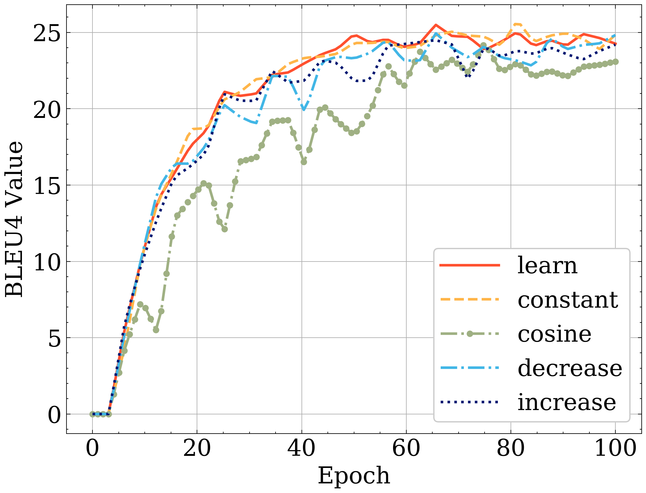
(a) Comparing various $\alpha$ strategies on PH14 dataset

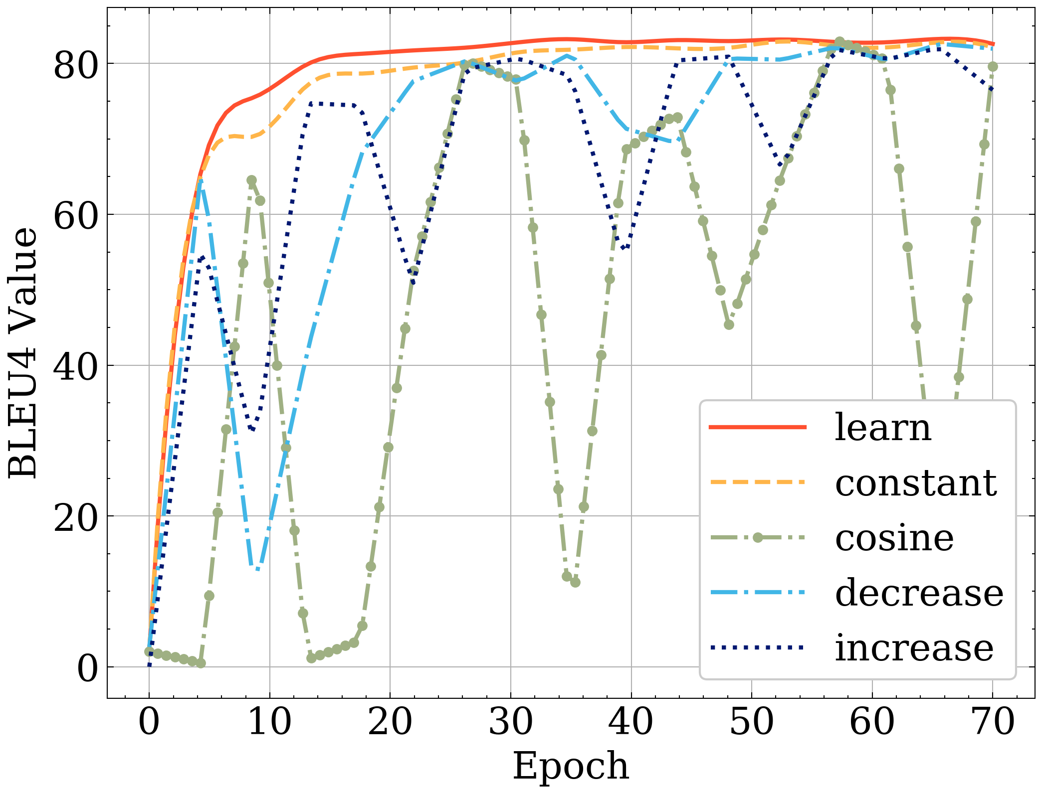
(b) Comparing various $\alpha$ strategies on ASLG dataset

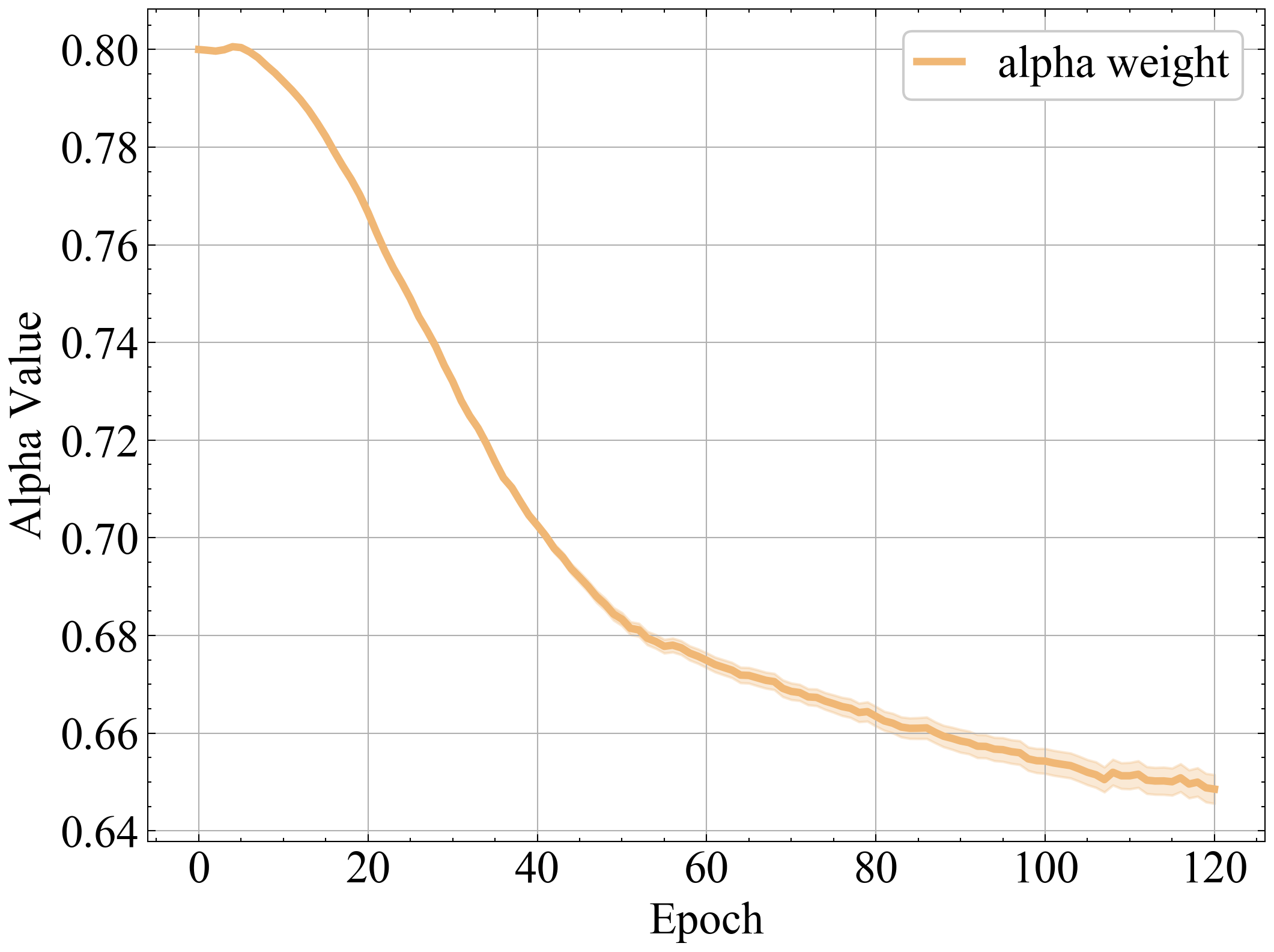
(c) The learned value of $\alpha$ on PH14 dataset

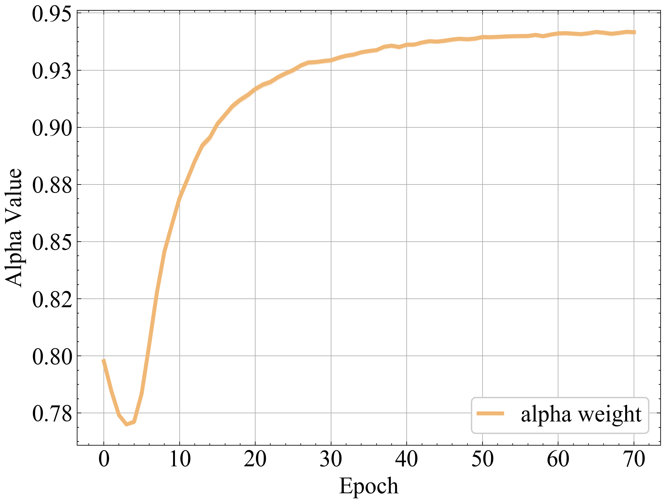
(d) The learned value of $\alpha$ on ASLG dataset

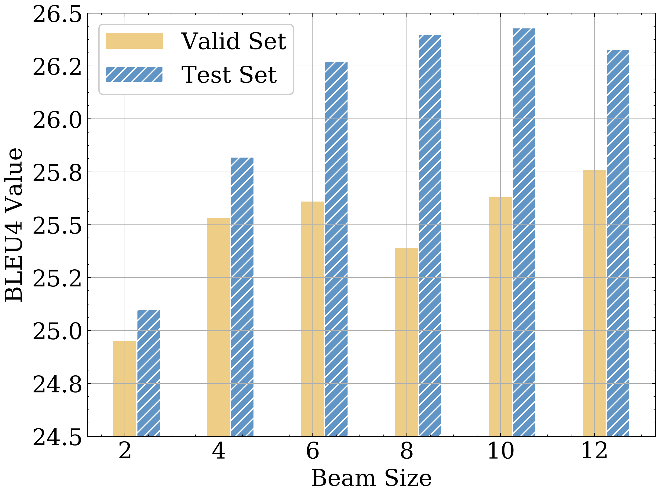
(e) Effect of beam size

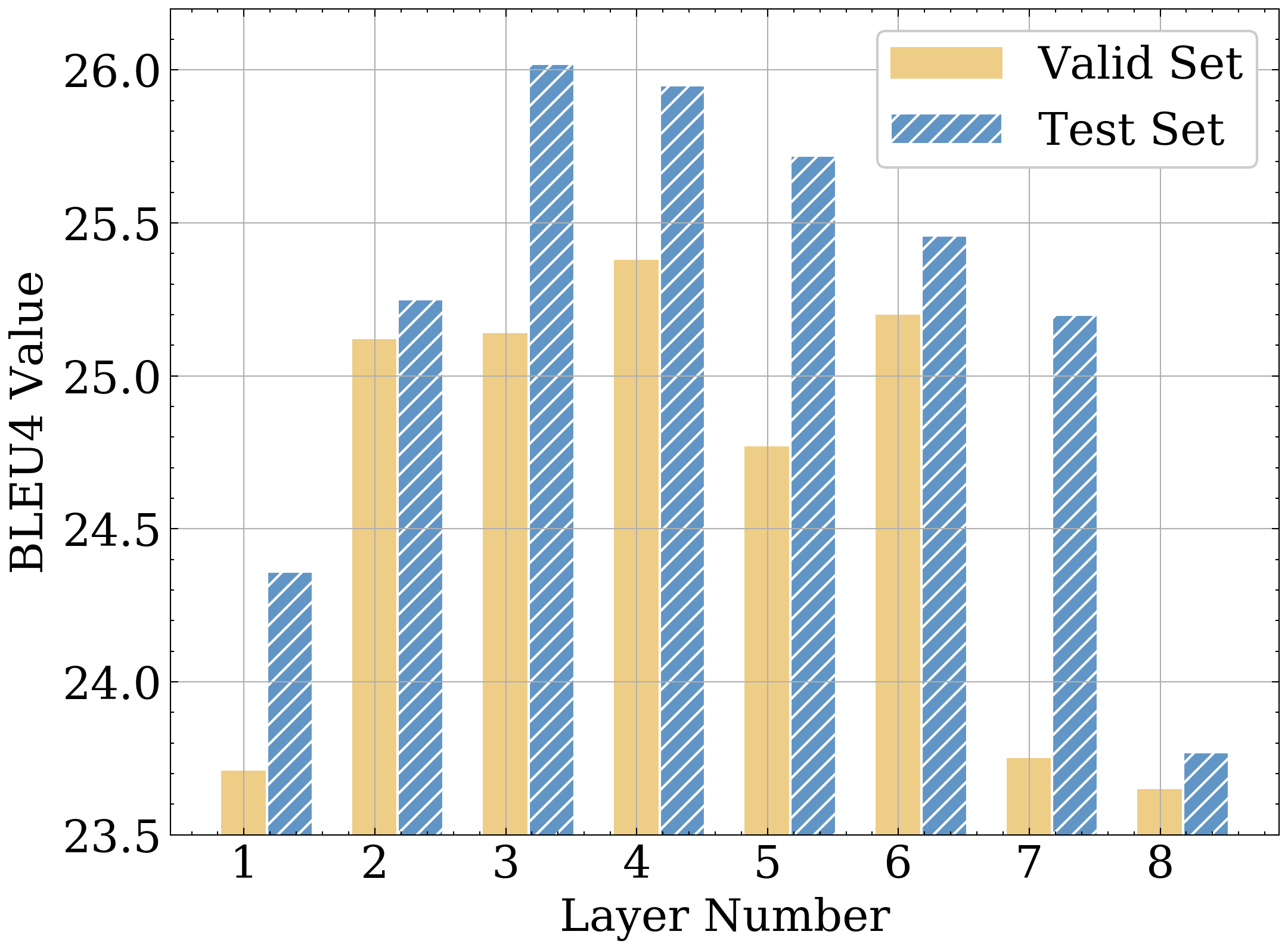
(f) Effect of layer number

(g) Effect of learning rate

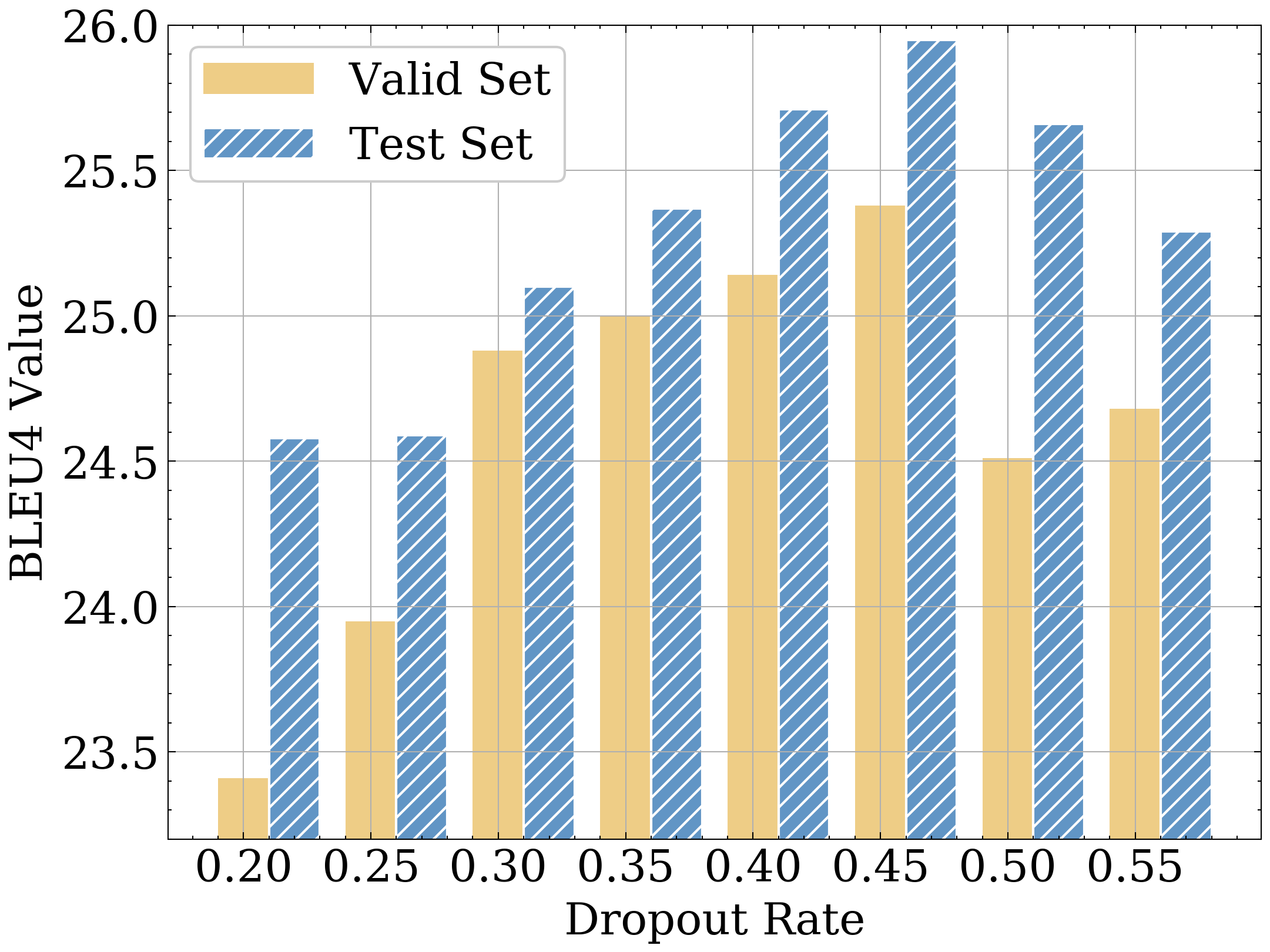
(h) Effect of dropout rate

Figure 5: Various analysis results. (a) & (b) present the results by using different feature fusion strategies on two datasets, respectively. (c) & (d) show our learned value of $\alpha$ during the training process on the two datasets, respectively. (e)-(h) explore how beam size, layer number, learning rate, and dropout rate affect the model performance.

Evaluation on S2G2T.  S2G2T is an extended task beyond G2T, which aims to recognize sign language videos to sign glosses, and then translate the recognized glosses to spoken sentences. Hence, unlike the task of G2T, in this comparison, we focus on the evaluation of the whole two-step pipeline, that is, obtaining spoken language sentences from sign language videos. Considering that only PH14 contains sign language videos, we thus conduct experiments on this dataset for S2G2T task, and the results are reported in Table 2. Note that, for the recognition step, we employ STMC model to realize vision-based sequence learning (Zhou et al., 2020). From the comparison we can see that, our TIN-SLT still outperforms existing approaches on most evaluation metrics.

			Test Set
Model	BLEU-1	BLEU-2	BLEU-3	BLEU-4	ROUGL-L	METEOR
G2T	44.13	31.47	23.89	19.26	45.45	-
S2G-G2T	41.54	29.52	22.24	17.79	43.45	-
S2G2T	43.29	30.39	22.82	18.13	43.80	-
Sign2	46.61	33.73	26.19	21.32	-	-
Bahdanau	47.53	33.82	26.07	21.54	45.50	44.87
Luong	47.08	33.93	26.31	21.75	45.66	44.84
Transformer Ens.	50.63	38.36	30.58	25.40	48.78	47.60
TIN-SLT (Ours)	51.06	38.85	31.23	26.13	48.56	47.83

Table 2: Comparing the S2G2T performance by using our TIN-SLT and state-of-the-art techniques on PHOENIX-2014-T dataset. The results of G2T, S2G-G2T and S2G2T are from (Camgoz et al., 2018). The results of Sign2 are from (Camgoz et al., 2020). The results of Bahdanau, Luong, and Transformer Ens. are from (Yin and Read, 2020). Clearly, our TIN-SLT achieves the highest values on most metrics.

5.3 Analysis and Discussions

Here, we conducted a series of detailed experiments to analyze our method and give some insights behind our network design.

Effect of learning-based feature fusion.  In this work, we propose a learning-based strategy to set $\alpha$ dynamically. Here, we conducted experiments by comparing this strategy with other four different strategies, including (1) cosine annealing (Loshchilov and Hutter, 2016), (2) cosine increment, (3) cosine decrement, and (4) constant value. The update of $\alpha$ by the three cosine strategies are calculated as Eq. (11) with different settings of the epoch cycle coefficient $T_{c}$:

$$\alpha_{t+1}=\alpha_{min}+\frac{1}{2}(\alpha_{max}-\alpha_{min})(1-cos(\frac{T_{t}}{T_{c}}\pi+\gamma))$$ (11)

where $\alpha$ is the fusion ratio, $T_{t}$ is current epoch step, and $\gamma$ is the time-shift constant. We set $T_{c}$ as (25, 100, 100) and $\gamma$ as (0, 0, $\pi$) for cosine annealing, cosine decrement, and cosine increment, respectively. The minimum value $\alpha_{min}$ and maximum value $\alpha_{max}$ of $\alpha$ are set to be 0 and 1.

Figures 5(a)-5(b) are the experimental results on the two datasets. We can observe that the learning-based strategy (red line) gets the best result on ASLG and comparable result with the constant setting ($\alpha$$=$$0.8$) on PH14, but still better than other three cosine strategies. Moreover, we also visualize the learned value of $\alpha$ during the training process as shown in Figures 5(c)-5(d) to find out the contribution ratio of the BERT model to the final performance. We can see that, the value of $\alpha$ is gradually decreasing on PH14, meaning that the model depends more on the BERT pre-trained knowledge at the beginning of the training process and gradually inclines to our employed training corpus. The observation is just opposite on ASLG, since it is a much larger dataset than PH14 and our model relies more on BERT to further boost the performance near the end of training.

			Test Set
Model	BLEU-1	BLEU-2	BLEU-3	BLEU-4	ROUGE-L	METEOR
	PHOENIX-2014-T Dataset Evaluation
Baseline	47.69	35.52	28.17	23.32	46.58	44.85
w/ DataAug	50.77	37.85	29.88	24.57	47.39	46.95
w/ Encoder	51.05	37.94	29.91	24.63	47.59	47.13
w/ Decoder	50.99	38.47	30.48	25.08	48.78	48.20
Full pipeline	52.77	40.08	32.09	26.55	49.43	49.36
	ASLG-PC12 Dataset Evaluation
Baseline	92.98	89.09	85.63	82.41	95.87	96.46
w/ DataAug	92.60	89.15	85.80	83.05	95.08	95.33
w/ Encoder	92.77	89.22	86.23	83.40	95.22	96.87
w/ Decoder	93.15	89.80	86.49	83.89	95.34	95.67
Full pipeline	93.35	90.03	87.07	84.29	95.39	95.92

Table 3: Ablation analysis of our major network components on the G2T task.

Analysis on major network components.  In our TIN-SLT, there are two major components: the multi-level data augmentation scheme and the instruction module. To validate the effectiveness of each component, we conduct an ablation analysis on the G2T task with the following cases.

• Baseline: We use two layers Transformer (Yin and Read, 2020) without data augmentation and instruction module as baseline.

• w/ DataAug: Based on the baseline, we add our data augmentation scheme back.

• w/ Encoder: Based on w/ DataAug, we fuse instruction module only into the encoder.

• w/ Decoder: Based on w/ DataAug, we fuse instruction module only into the decoder.

As a contrast, in our full pipeline, the instruction module is inserted into both encoder and decoder. Table 3 shows the evaluation results on both PH14 and ASLG. By comparing the results from Baseline and w/ DataAug, we can see that our data augmentation improves the translation performance, especially for the PH14 dataset. A reasonable interpretation is that the translation task on PH14 dataset is more difficult than on ASLG, thus our data augmentation contributes more. On the other hand, w/ Encoder, w/ Decoder and Full pipeline explore the best location to introduce PTM information into the model. Results in Table 3 show that our full model achieves the best performance. Particularly, by comparing the results from w/ Encoder and w/ Decoder against the results from SOTA methods (Tables 1 & 3), we can observe that as long as we employ the pre-trained model, no matter where it is inserted into the network, the performance is always better than existing methods.

Model	Size(MB)	Dataset	Gloss(%)	Text(%)	BLEU4
	PHOENIX-2014-T Dataset Evaluation
Multilingual	641.10	PH14	59.96	74.62	25.48
Distilbert	257.30	PH14	44.50	71.15	24.73
Gbert	421.80	PH14	44.50	71.15	25.13
Dbmdz	421.80	PH14	73.72	88.13	26.55
	ASLG-PC12 Dataset Evaluation
Base-Tiny	16.90	ASLG	76.77	96.35	82.44
Electra	51.70	ASLG	76.77	96.35	82.60
Distilbert	255.60	ASLG	76.77	96.35	83.06
Base-uncased	420.10	ASLG	76.77	96.35	84.29

Table 4: Comparing different pre-trained models in terms of BLEU-4.

Effect of different pre-trained models.  We here explored the translation performance by using different pre-trained models; see Table 4. We analyzed the model size and vocabulary coverage of the pre-trained model with gloss and text of our dataset. We can see that introducing a pre-trained model with larger vocabulary coverage of the target dataset will gain better performance, since a pre-trained model with larger vocabulary coverage can inject more knowledge learned from another unlabeled corpus into the translation task. For ASLG, although the vocabulary coverage is the same, we can see that the bigger model has better performance since it can learn contextual representation better.

Analysis on hyper-parameters.  To search the best settings of our hyper-parameters, we employed Neural Network Intelligence (NNI) (Microsoft, 2018), a lightweight but powerful toolkit. As shown in Figures 5(e)-5(h), we explored how beam size, layer number, learning rate and dropout rate affect the model performance on PH14 dataset. First, beam search enables to explore more possible candidates, but large beam widths do not always result in better performance as shown in Figure 5(e). We obtain optimal beam size as 10 on PH14. Second, the layer number decides the model size and capacity, where the larger model would overfit on a small dataset. In Figure 5(f), we find the optimal layer number to be 3 on PH14. Lastly, as shown in Figures 5(g) & 5(h), we adopt an early-stopping strategy to avoid overfitting and find the best learning rate and dropout rate are 0.0003 and 0.45, respectively.

Case study.  Table 5 presents some intuitive translation results on ASLG by reporting the translated spoken sentences. Overall, the translation quality is good, even the translated sentences with low BLEU-4 still convey the same information. Also, we can observe that our translated sentences are basically the same with ground truth, although using different expressions, i.e., “decision making” vs. “decision made”. The translation results on PH14 are reported in Appendix.

Type	Content	BLEU-4
GT Gloss	X-IT BE DESC-UP TO X-YOU TO CONSIDER	100.00
	AND CHOOSE OUTCOME X-YOU WANT TO SEE .
GT Text	it is up to you to consider and choose
	the outcome you want to see .
Pred Text	it is up to you to consider and choose
	the outcome you want to see .
GT Gloss	X-I WANT IRELAND TO REMAIN AT	57.58
	HEART DECISION MAKE IN EUROPE .
GT Text	i want ireland to remain at the
	heart of decision making in europe .
Pred Text	i want ireland to remain at the
	heart of the decision made in europe .
GT Gloss	X-I WILL DESC-NEVER FORGET WHAT X-I	13.44
	EXPERIENCE . SHOULD BE ABOUT .
GT Text	that is what this european day of memorial should be
	about . i will never forget what i experienced .
Pred Text	i will never forget what i experienced .

Table 5: Qualitative evaluation of translation performance in different BLEU-4 scores on ASLG dataset.

6 Conclusion

In this paper, we proposed a task-aware instruction network for sign language translation. To address the problem of limited data for SLT, we introduced a pre-trained model into Transformer and designed an instruction module to adapt SLT task. Besides, due to the discrepancy between the representation space of sign glosses and spoken sentences, we proposed a multi-level data augmentation scheme. Extensive experiments validate our superior performance compared with state-of-the-art approaches. While there is obvious improvement among most evaluation metrics, the complexity of our models is also increased, causing a longer training period. In the future, we would like to explore the possibility of designing a lightweight model to achieve real-time efficiency.

Appendix A Appendix

A.1 Dataset Description

In this section, we will introduce two public benchmark datasets used in sign language translation tasks, namely PHOENIX-2014-T and ASLG-PC12. We conducted statistical analysis on the datasets and the results are shown in Table 6. It is obvious that PHOENIX-2014-T is a small-scale dataset, while ASLG-PC12 is a large-scale dataset.

Dataset		Gloss			Translation
		Train	Dev	Test	Train	Dev	Test
PH14	Samples	7096	519	642	7096	519	642
	Vocabs	1066	393	411	2887	951	1001
	Words	67781	3745	4257	99081	6820	7816
ASLG	Samples	82709	4000	1000	82709	4000	1000
	Vocabs	15782	4323	2150	21600	5634	2609
	Words	862046	41030	10503	975942	46637	11953

Table 6: The descriptive statistics of PHOENIX-2014-T and ASLG-PC12 datasets. Samples row means the sample size of the dataset, Vocabs row represents the total vocabularies contained in the dataset, and Words row means the total words of the dataset.

A.2 PHOENIX-2014-T Qulitative Result

BE-SLT performance of G2T task on PHOENIX-2014-T is shown in Table 7, from which we can observe that sign language translation results are of good quality with different BLEU-4 scores and the predicted sentences can convey effective information even for low BLEU-4 scores.

Type	Content	BLEU-4
Gloss	BERG ORKAN MOEGLICH	100.00
GT Text	auf den bergen sind orkanartige
	böen möglich .
Pred Text	auf den bergen sind orkanartige
	böen möglich .
Gloss	HEUTE NACHT ZWISCHEN NEUNZEHN ZWISCHEN	57.58
	FUENFZEHN SUEDOST MAXIMAL ZWOELF
GT Text	heute nacht werte zwischen neunzehn und fünfzehn
	grad im südosten bis zwölf grad .
Pred Text	heute nacht neunzehn bis fünfzehn grad im
	südosten bis zwölf grad .
Gloss	RUSSLAND IX TROCKEN HEISS SCHEINEN FUENF	13.44
	DREISSIG BIS VIERZIG GRAD
GT Text	ganz anders die trockene hitze über russland
	mit fünfunddreißig bis vierzig grad .
Pred Text	aber bei uns wird es auch noch ein bisschen
	heißer da sind es fünf bis vierzig grad .

Table 7: PHOENIX-2014-T: Qualitatively evaluation of translation performance in different BLEU-4 scores.

A.3 Experiment Parameter

In order to help reproduce BE-SLT and its translation performance, as shown in Table 8 and 9, we list the hyper-parameters of the best results on two benchmark datasets. For G2T task on PHOENIX-2014-T, we list the best hyper-parameter settings for the experiments which apply data augmentation scheme, or fuse BERT-attention module into encoder, decoder, and both respectively (namely,w/DataAug, w/Encoder, w/Decoder, w/All). W/All obtains the highest BLEU-4 using the initial learning rate of 0.00025, dropout rate of 0.45, beam search with width 5, and the max epoch size of 120. For G2T task on ASLG-PC12, we also list the hyper-parameter settings for the four experiments that achieve significant results, listed in Table 9. For more experiment details, please refer to our code which will be published upon the publication of this work.

		PHOENIX-2014-T
Parameter	w/DataAug	w/Encoder	w/Decoder	w/All
Embedding size	512	512	512	512
Hidden size	2048	2048	2048	2048
Head number	8	8	8	8
Encoder BERT gate	1	1	0	1
Decoder BERT gate	1	0	1	1
Optimizer	Adam	Adam	Adam	Adam
Learning rate	0.00025	0.00025	0.00025	0.0003
LR schedule	inverse sqrt	inverse sqrt	inverse sqrt	inverse sqrt
Weight decay	$10^{-3}$	$10^{-3}$	$10^{-3}$	$10^{-3}$
Drop out	0.45	0.45	0.45	0.45
Label smoothing	0.3	0.3	0.3	0.3
BERT ratio	-	0.6	0.6	0.65
Max epoch	120	120	120	120
BERT model	bert-base-german-dbmdz-uncased

Table 8: The hyper-parameters of the best results on PHOENIX-2014-T for the G2T task.

		ASLG-PC12
Parameter	w/DataAug	w/Encoder	w/Decoder	w/All
Embedding size	512	512	512	512
Hidden size	2048	2048	2048	2048
Head number	8	8	8	8
Encoder BERT gate	1	1	0	1
Decoder BERT gate	1	0	1	1
Optimizer	Adam	Adam	Adam	Adam
Learning rate	0.00025	0.00025	0.00025	0.00045
LR schedule	inverse sqrt	inverse sqrt	inverse sqrt	inverse sqrt
Weight decay	$10^{-3}$	$10^{-3}$	$10^{-3}$	$10^{-3}$
Drop out	0.45	0.45	0.45	0.4
Label smoothing	0.3	0.3	0.3	0.1
BERT ratio	-	0.6	0.6	0.6
Max epoch	70	70	70	70
BERT model	bert-base-uncased

Table 9: The hyper-parameters of the best results on ASLG-PC12 for the G2T task.

A.4 Alpha Strategy Settings

Here we introduce the $\alpha$ value setting details corresponding to cosine strategy and constant strategy adopted in this work as shown in Formula 2 and Formula 4. The cosine annealing and cosine decrement strategies are calculated according to Formula 11. To simplify the calculation, the cosine increment strategy is calculated according to Formula 12. In order to be more intuitive, we plotted the curve of $\alpha$ value during the training process, as shown in Figure 6.

$$\alpha_{t+1}=1-\alpha_{min}-\frac{1}{2}(\alpha_{max}-\alpha_{min})(1-cos(\frac{T_{t}}{T_{c}}\pi))$$ (12)

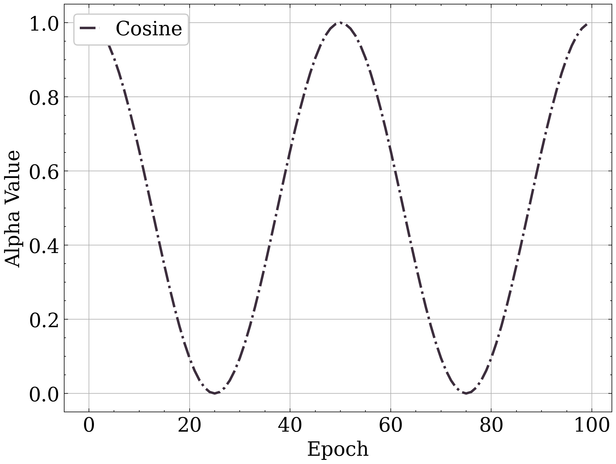
(a) Cosine annealing strategy

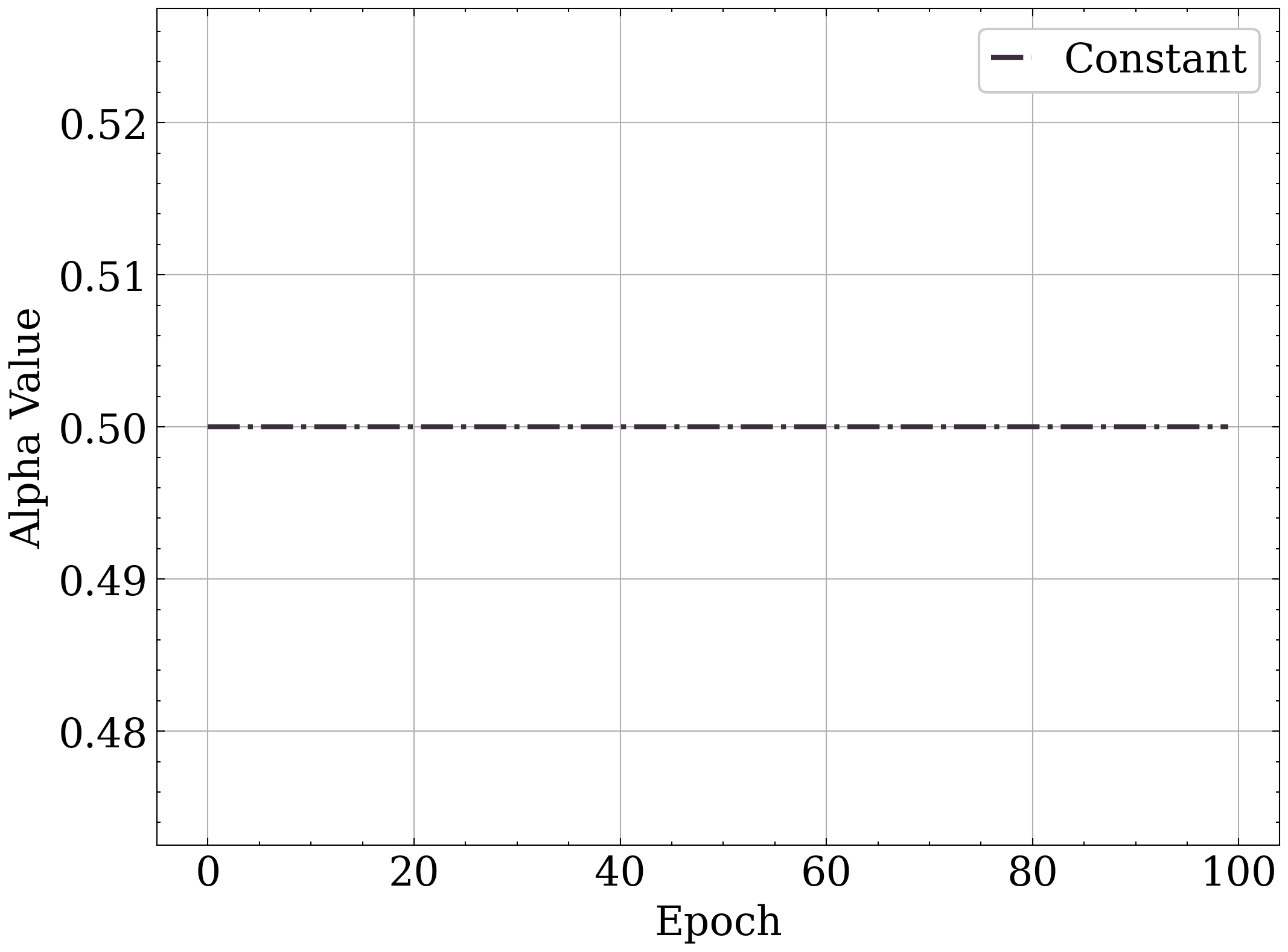
(b) Constant strategy

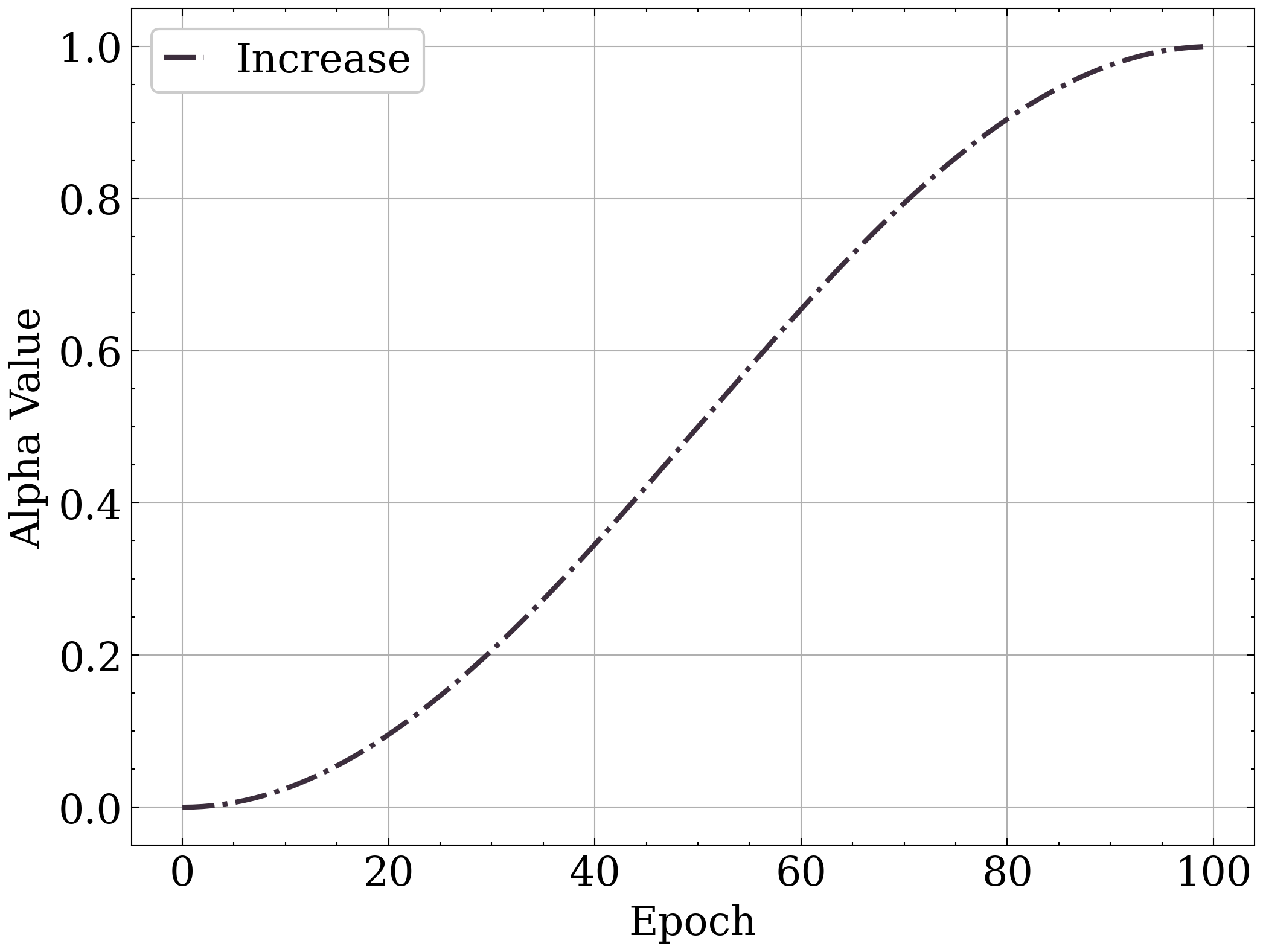
(c) Cosine increment strategy

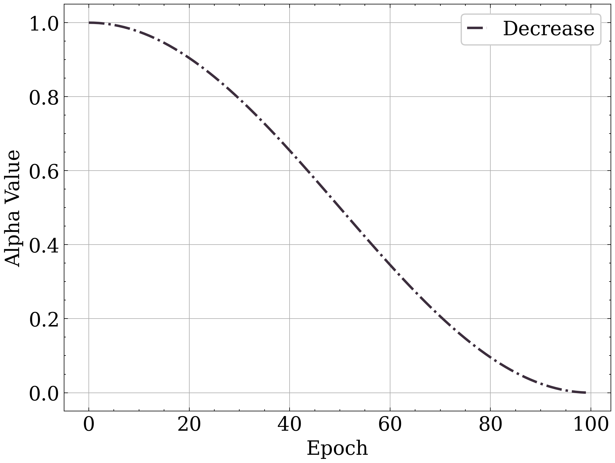
(d) Cosine decrement strategy

Figure 6: The $\alpha$ value during the training process in four setting strategies, namely cosine annealing, cosine increment, cosine decrement and constant.

A.5 Pre-trained Models Download

All BERT pre-trainied models adopted in Table 4 are published by (Huggingface-community, 2018). In order to help reproduce our work and use our code easily, we summarize the download links of the pre-trained models as follows.

PHOENIX-2014-T Dataset

• Multilingual: bert-base-multilingual-uncased
  https://huggingface.co/bert-base-multilingual-uncased

• Distilbert: distilbert-base-german-cased
  https://huggingface.co/distilbert-base-german-cased

• Gbert: gbert-base
  https://huggingface.co/deepset/gbert-base

• Dbmdz: bert-base-german-dbmdz-uncased
  https://huggingface.co/bert-base-german-dbmdz-uncased

ASLG-PC12 Dataset

• Base-Tiny: bert-tiny
  https://huggingface.co/prajjwal1/bert-tiny

• Electra: electra-small-discriminator
  https://huggingface.co/google/electra-small-discriminator

• Distilbert: distilbert-base-uncased
  https://huggingface.co/distilbert-base-uncased

• Base-uncased: bert-base-uncased
  https://huggingface.co/bert-base-uncased

References

- Arvanitis et al. (2019) Nikolaos Arvanitis, Constantinos Constantinopoulos, and Dimitrios Kosmopoulos. 2019. Translation of sign language glosses to text using sequence-to-sequence attention models. In 2019 15th International Conference on Signal-Image Technology & Internet-Based Systems (SITIS), pages 296–302. IEEE.
- Bahdanau et al. (2014) Dzmitry Bahdanau, Kyunghyun Cho, and Yoshua Bengio. 2014. Neural machine translation by jointly learning to align and translate. arXiv preprint arXiv:1409.0473.
- Banerjee and Lavie (2005) Satanjeev Banerjee and Alon Lavie. 2005. Meteor: An automatic metric for mt evaluation with improved correlation with human judgments. In Proceedings of the acl workshop on intrinsic and extrinsic evaluation measures for machine translation and/or summarization, pages 65–72.
- Bragg et al. (2019) Danielle Bragg, Oscar Koller, Mary Bellard, Larwan Berke, Patrick Boudreault, Annelies Braffort, Naomi Caselli, Matt Huenerfauth, Hernisa Kacorri, Tessa Verhoef, et al. 2019. Sign language recognition, generation, and translation: An interdisciplinary perspective. In The 21st international ACM SIGACCESS conference on computers and accessibility, pages 16–31.
- Camgoz et al. (2018) Necati Cihan Camgoz, Simon Hadfield, Oscar Koller, Hermann Ney, and Richard Bowden. 2018. Neural sign language translation. In Proceedings of the IEEE Conference on Computer Vision and Pattern Recognition, pages 7784–7793.
- Camgoz et al. (2020) Necati Cihan Camgoz, Oscar Koller, Simon Hadfield, and Richard Bowden. 2020. Sign language transformers: Joint end-to-end sign language recognition and translation. In Proceedings of the IEEE/CVF conference on computer vision and pattern recognition, pages 10023–10033.
- Cui et al. (2019) Runpeng Cui, Hu Liu, and Changshui Zhang. 2019. A deep neural framework for continuous sign language recognition by iterative training. IEEE Transactions on Multimedia, 21(7):1880–1891.
- Gehring et al. (2017) Jonas Gehring, Michael Auli, David Grangier, Denis Yarats, and Yann N Dauphin. 2017. Convolutional sequence to sequence learning. In International Conference on Machine Learning, pages 1243–1252. PMLR.
- Huggingface-community (2018) Huggingface-community. 2018. https://huggingface.co/models. Accessed: 2018-11-17.
- Imamura and Sumita (2019) Kenji Imamura and Eiichiro Sumita. 2019. Recycling a pre-trained bert encoder for neural machine translation. In Proceedings of the 3rd Workshop on Neural Generation and Translation, pages 23–31.
- Kingma and Ba (2014) Diederik P Kingma and Jimmy Ba. 2014. Adam: A method for stochastic optimization. arXiv preprint arXiv:1412.6980.
- Ko et al. (2019) Sang-Ki Ko, Chang Jo Kim, Hyedong Jung, and Choongsang Cho. 2019. Neural sign language translation based on human keypoint estimation. Applied Sciences, 9(13):2683.
- Koller et al. (2019) Oscar Koller, Necati Cihan Camgoz, Hermann Ney, and Richard Bowden. 2019. Weakly supervised learning with multi-stream cnn-lstm-hmms to discover sequential parallelism in sign language videos. IEEE transactions on pattern analysis and machine intelligence, 42(9):2306–2320.
- Koller et al. (2017) Oscar Koller, Sepehr Zargaran, and Hermann Ney. 2017. Re-sign: Re-aligned end-to-end sequence modelling with deep recurrent cnn-hmms. In Proceedings of the IEEE Conference on Computer Vision and Pattern Recognition (CVPR).
- Kumar et al. (2020) E Kiran Kumar, PVV Kishore, M Teja Kiran Kumar, and D Anil Kumar. 2020. 3d sign language recognition with joint distance and angular coded color topographical descriptor on a 2–stream cnn. Neurocomputing, 372:40–54.
- Li et al. (2020) Dongxu Li, Cristian Rodriguez, Xin Yu, and Hongdong Li. 2020. Word-level deep sign language recognition from video: A new large-scale dataset and methods comparison. In Proceedings of the IEEE/CVF winter conference on applications of computer vision, pages 1459–1469.
- Lin (2004) Chin-Yew Lin. 2004. Rouge: A package for automatic evaluation of summaries. In Text summarization branches out, pages 74–81.
- Loshchilov and Hutter (2016) Ilya Loshchilov and Frank Hutter. 2016. Sgdr: Stochastic gradient descent with warm restarts. arXiv preprint arXiv:1608.03983.
- Microsoft (2018) Microsoft. 2018. https://github.com/microsoft/nni. Accessed: 2018-09-20.
- Mikolov et al. (2013) Tomas Mikolov, Ilya Sutskever, Kai Chen, Greg S Corrado, and Jeff Dean. 2013. Distributed representations of words and phrases and their compositionality. In Advances in neural information processing systems, pages 3111–3119.
- Moryossef et al. (2021) A. Moryossef, K. Yin, G. Neubig, and Y. Goldberg. 2021. Data augmentation for sign language gloss translation.
- Othman and Jemni (2012) Achraf Othman and Mohamed Jemni. 2012. English-asl gloss parallel corpus 2012: Aslg-pc12. In 5th Workshop on the Representation and Processing of Sign Languages: Interactions between Corpus and Lexicon LREC.
- Papineni et al. (2002) Kishore Papineni, Salim Roukos, Todd Ward, and Wei-Jing Zhu. 2002. Bleu: a method for automatic evaluation of machine translation. In Proceedings of the 40th annual meeting of the Association for Computational Linguistics, pages 311–318.
- Qiu et al. (2017) Zhaofan Qiu, Ting Yao, and Tao Mei. 2017. Learning spatio-temporal representation with pseudo-3d residual networks. In proceedings of the IEEE International Conference on Computer Vision, pages 5533–5541.
- Sharma and Kumar (2021) Shikhar Sharma and Krishan Kumar. 2021. Asl-3dcnn: American sign language recognition technique using 3-d convolutional neural networks. Multimedia Tools and Applications, pages 1–13.
- Shavarani and Sarkar (2021) Hassan S Shavarani and Anoop Sarkar. 2021. Better neural machine translation by extracting linguistic information from bert. arXiv preprint arXiv:2104.02831.
- Sincan and Keles (2020) Ozge Mercanoglu Sincan and Hacer Yalim Keles. 2020. Autsl: A large scale multi-modal turkish sign language dataset and baseline methods. IEEE Access, 8:181340–181355.
- Stoll et al. (2018) Stephanie Stoll, Necati Cihan Camgöz, Simon Hadfield, and Richard Bowden. 2018. Sign language production using neural machine translation and generative adversarial networks. In Proceedings of the 29th British Machine Vision Conference (BMVC 2018). University of Surrey.
- Sutskever et al. (2014) Ilya Sutskever, Oriol Vinyals, and Quoc V Le. 2014. Sequence to sequence learning with neural networks. In Advances in neural information processing systems, pages 3104–3112.
- Vaswani et al. (2017) Ashish Vaswani, Noam Shazeer, Niki Parmar, Jakob Uszkoreit, Llion Jones, Aidan N Gomez, Łukasz Kaiser, and Illia Polosukhin. 2017. Attention is all you need. In Advances in neural information processing systems, pages 5998–6008.
- Wei et al. (2019) Chengcheng Wei, Wengang Zhou, Junfu Pu, and Houqiang Li. 2019. Deep grammatical multi-classifier for continuous sign language recognition. In 2019 IEEE Fifth International Conference on Multimedia Big Data (BigMM), pages 435–442. IEEE.
- Yin et al. (2016) Fang Yin, Xiujuan Chai, and Xilin Chen. 2016. Iterative reference driven metric learning for signer independent isolated sign language recognition. In European Conference on Computer Vision, pages 434–450. Springer.
- Yin et al. (2021) K. Yin, A. Moryossef, J. Hochgesang, Y. Goldberg, and M. Alikhani. 2021. Including signed languages in natural language processing. In Proceedings of the 59th Annual Meeting of the Association for Computational Linguistics and the 11th International Joint Conference on Natural Language Processing (Volume 1: Long Papers).
- Yin and Read (2020) Kayo Yin and Jesse Read. 2020. Better sign language translation with stmc-transformer. arXiv preprint arXiv:2004.00588.
- Zhou et al. (2020) Hao Zhou, Wengang Zhou, Yun Zhou, and Houqiang Li. 2020. Spatial-temporal multi-cue network for continuous sign language recognition. In Proceedings of the AAAI Conference on Artificial Intelligence, volume 34, pages 13009–13016.
- Zhu et al. (2020) Jinhua Zhu, Yingce Xia, Lijun Wu, Di He, Tao Qin, Wengang Zhou, Houqiang Li, and Tie-Yan Liu. 2020. Incorporating bert into neural machine translation. arXiv preprint arXiv:2002.06823.