Improved data analysis on two-point correlation function with sequential Bayesian method

Abstract

We report our progress in data analysis on two-point correlation functions of the $B$ meson using sequential Bayesian method. The data set of measurement is obtained using the Oktay-Kronfeld (OK) action for the bottom quarks (valence quarks) and the HISQ action for the light quarks on the MILC HISQ lattices. We find that the old initial guess for the $\chi^{2}$ minimizer in the fitting code is poor enough to slow down the analysis somewhat. In order to find a better initial guess, we adopt the Newton method. We find that the Newton method provides a natural test to check whether the $\chi^{2}$ minimizer finds a local minimum or the global minimum, and it also reduces the number of iterations dramatically.

1 Introduction

To determine Cabibbo-Kobayashi-Maskawa (CKM) matrix element $|V_{cb}|$, we need to calculate the semileptonic form factors for the $\bar{B}\to D^{\ast}\ell\bar{\nu}$ and $\bar{B}\to D\ell\bar{\nu}$ decays on the lattice. In order to obtain the semileptonic form factors, we need to do the data analysis on the three-point (3pt) correlation functions, which require results for the masses and normalization constants obtained from the two-point (2pt) correlation functions. Here, we present recent progress in our data analysis on the 2pt correlation functions to determine the masses and normalization constants for the ground and excited states.

We adopt the Fermilab formulation [1] to implement the heavy quarks such as bottom and charm quarks on the lattice. The Fermilab action [1] is improved up to the $\lambda^{1}$ level ($\lambda\simeq\Lambda/(2m_{Q})$), and so it is impossible to achieve a sub-percent precision with it by construction. In order to overcome this difficulty, we use the Oktay-Kronfeld (OK) action [2] improved up to the $\lambda^{3}$ level. Recently, we have completed the current improvement up to the same level as the OK action [3].

The OK action for a heavy quark is

$$S_{\text{OK}} =S_{0}+S_{1}+S_{2}+S_{3}$$ (1)

where $S_{n}$ represents those $\mathcal{O}(\lambda^{n})$ terms of $S_{\text{OK}}$ collectively.

$$S_{0} =a^{4}\sum_{x}\bar{\psi}(x)\left[m_{0}+\gamma_{4}D_{4}\right]\psi(x)\,,$$

$$S_{1} =a^{4}\sum_{x}\bar{\psi}(x)\left[-\frac{1}{2}a\Delta_{4}+\zeta\bm{\gamma\cdot D}-\frac{1}{2}r_{s}\zeta a\Delta^{(3)}-\frac{1}{2}c_{B}a\zeta i\bm{\Sigma\cdot B}\right]\psi(x)\,,$$

$$S_{2} =a^{4}\sum_{x}\bar{\psi}(x)\left[-\frac{1}{2}c_{E}a\zeta\bm{\alpha\cdot E}\right]\psi(x)\,,$$

$$S_{3} =a^{4}\sum_{x}\bar{\psi}(x)\left[c_{1}a^{2}\sum_{k}\gamma_{k}D_{k}\Delta_{k}+c_{2}a^{2}\{\bm{\gamma\cdot D},\Delta^{(3)}\}+c_{3}a^{2}\{\bm{\gamma\cdot D}\,,i\bm{\Sigma\cdot B}\}\right.$$

$$\hphantom{=a^{4}\sum_{x}\bar{\psi}(x)[\ }\left.+c_{EE}a^{2}\{\gamma_{4}D_{4}\,,\bm{\alpha\cdot E}\}+c_{4}a^{3}\sum_{k}\Delta_{k}^{2}+c_{5}a^{3}\sum_{k}\sum_{j\neq k}\{i\Sigma_{k}B_{k}\,,\Delta_{j}\}\right]\psi(x)\,.$$ (2)

Here, we use the same notation as in Ref. [2]. The bare quark mass $m_{0}$ is

$$am_{0}=\frac{1}{2}\left(\frac{1}{\kappa}-\frac{1}{\kappa_{\text{crit}}}\right)\,,$$ (3)

where $\kappa$ ($\kappa_{\text{crit}}$) is a (critical) hopping parameter [4]. Numerical values for $\kappa$ and $\kappa_{\text{crit}}$ are summarized in Table 1. We use the HISQ action [5] for strange quarks.

In order to get a better signal for the $B_{s}$ meson states, we apply a covariant Gaussian smearing (CGS), $\left\{1+\sigma^{2}\nabla^{2}/(4N_{\text{GS}})\right\}^{N_{\text{GS}}}$ to the point source and sink as in Ref. [6]. The CGS parameters are summarized in Table 1. We apply the CGS only to the heavy quark fields and not to the light quark fields.

$m_{x}/m_{s}$	$\kappa_{\text{crit}}$	$\kappa_{b}$	$\{\sigma\,,\;N_{\text{GS}}\}$	$N_{\text{cfg}}\times N_{\text{src}}$
1	0.051218	0.04070	$\{1.5\,,\;5\}$	$1000\times 3$

Table 1: Hopping parameters and smearing parameters. Here, $m_{x}$ is a mass of valence light quarks. $N_{\text{cfg}}$ represents the number of gauge configurations and $N_{\text{src}}$ is the number of sources per gauge configuration.

We use the MILC HISQ ensembles with $N_{f}=2+1+1$ [7]. The details are summarized in Table 2.

$a$ (fm)	$N_{s}^{3}\times N_{t}$	$M_{\pi}$ (MeV)	$am_{l}$	$am_{s}$	$am_{c}$
0.1184(10)	$32^{3}\times 64$	216.9(2)	0.00507	0.0507	0.628

Table 2: Details on the MILC HISQ ensembles with $N_{f}=2+1+1$ [7].

2 Sequential Bayesian Method

Let us consider 2pt correlation functions [8]:

$$C(t) =\sum_{\alpha=1}^{4}\sum_{\bf{x}}\langle\mathcal{O}^{\dagger}_{\alpha}(t,{\bf x})\mathcal{O}_{\alpha}(0)\rangle$$ (4)

Here, the interpolating operator for the heavy-light meson is

$$\mathcal{O}_{\alpha}(t,{\bf x}) =\left[\bar{\psi}_{b}(t,{\bf x})\gamma_{5}\Omega(t,{\bf x})\right]_{\alpha}\chi_{\ell}(t,{\bf x})\,.$$ (5)

Here $\psi_{b}$ is an OK action field for bottom quarks, and $\chi_{\ell}$ is an HISQ action field for light quarks.

$$\Omega(t,{\bf x})\equiv\gamma_{1}^{\;x_{1}}\gamma_{2}^{\;x_{2}}\gamma_{3}^{\;x_{3}}\gamma_{4}^{\;t}\,.$$ (6)

The subscript $\alpha$ represents taste degrees of freedom for staggered light quarks.

We construct the fitting function to contain $m$ even time-parity states and $n$ odd time-parity states, which we call “$m+n$ fit”. The $m+n$ fit function is

$$f(t) =g(t)+g(T-t)\,,$$

$$g(t) =A_{0}\,e^{-E_{0}\,t}\left[1+R_{2}\,e^{-\Delta E_{2}\,t}\left(1+R_{4}\,e^{-\Delta E_{4}\,t}\left(\cdots\left(1+R_{2m-2}\,e^{-\Delta E_{2m-2}\,t}\right)\cdots\right)\right)\right.$$

$$\hphantom{=A_{0}\,e^{-E_{0}\,t}[\ }\left.-(-1)^{t}\,R_{1}\,e^{-\Delta E_{1}\,t}\left(1+R_{3}\,e^{-\Delta E_{3}\,t}\left(\cdots\left(1+R_{2n-1}\,e^{-\Delta E_{2n-1}\,t}\right)\cdots\right)\right)\right]$$ (7)

where $\Delta E_{i}\equiv E_{i}-E_{i-2}$, $E_{-1}\equiv E_{0}$ , $R_{i}\equiv{A_{i}}/{A_{i-2}}$ and $A_{-1}\equiv A_{0}$.

We adopt the sequential Bayesian method for fitting. We take the following steps to analyze the 2-point correlation functions.

Step 1

Do the 1st fitting.  ex) 1+0 fit (2 parameters: {$A_{0}$, $E_{0}$})

Step 2

Feed the fitting results as prior information for the 2nd fitting.
ex) 1+1 fit (4 parameters: {$A_{0}$, $E_{0}$, $R_{1}$, $\Delta E_{1}$}, 2 prior information on {$A_{0}$, $E_{0}$})

Step 3

Do stability test and find optimal prior information. ex) stability test gives optimal prior information on {$A_{0}$, $E_{0}$}.

Step 4

Save the 2nd fitting results (e.g. 1+1 fit) into the 1st fitting.

Step 5

Choose the next fitting (e.g. 2+1 fit) as the 2nd fitting.

Step 6

Go back to Step 2.  ex) 1+0 $\to$ 1+1 $\to$ 2+1 $\to$ 2+2 $\to$ $\cdots$.

3 Numerical precision problem on covariance matrix inversion

When we fit the data to the fitting function given in Eq. (7), we encounter a numerical precision problem in the covariance matrix inversion. For example, we set the fitting range to $15\leq t\leq 29$ and then we have a covariance matrix $V$ of $15\times 15$. We use the Cholesky decomposition algorithm to obtain the inverse matrix $V^{-1}$. In order to check the matrix inversion, we monitor the following identity: $V\cdot V^{-1}=1$. If everything works well, we will get the off-diagonal components of $V\cdot V^{-1}$ to be zero within numerical precision, but we find that some of them are $\mathcal{O}(10^{-5})$. We also find that the largest and smallest eigenvalues for $V$ are $\mathcal{O}(10^{-35})$ and $\mathcal{O}(10^{-60})$, respectively. Since $V^{-1}$ is used multiple times in the least $\chi^{2}$ fitting, we need $V^{-1}$ accurate up to double precision, but the existing fitting code cannot achieve the numerical precision. Hence, we find two independent methods to resolve the puzzle: one is the rescaling method and the other the correlation matrix method.

3.1 Rescaling method

We transform the data $C(t)$, the fit function $f(t)$ and the covariance matrix $V(t_{i},t_{j})$ by an arbitrary rescaling factor $R(t)$ as follows,

$$\tilde{C}(t) =\frac{C(t)}{R(t)}\,,\quad\tilde{f}(t)=\frac{f(t)}{R(t)}\,,\quad\tilde{V}(t_{i},t_{j})=\frac{V(t_{i},t_{j})}{R(t_{i})\,R(t_{j})}\,.$$ (8)

Then the fitting results and the $\chi^{2}$ value are invariant under the rescaling transformation of Eqs. (8), regardless of details on $R(t)$. Here, note that the fitting parameters never be changed by the rescaling factor $R(t)$.

In our data analysis, we set the rescaling function to

$$R(t) =A_{0}^{r}\exp[-E_{0}^{r}t]+A_{0}^{r}\exp[-E_{0}^{r}(T-t)]\,.$$ (9)

Here, $A_{0}^{r}$ and $E_{0}^{r}$ is determined by fitting the data in the fit range ($23\leq t\leq 29$), where the superscript $r$ represents the rescaling function. The huge scale difference between the largest and the smallest eigenvalues of $V$ comes from the large mass ($E_{0}\simeq 2.0/a$) of the $B_{s}$ meson, since the 2pt correlation function decreases as a function of $\sim\exp(-E_{0}t)$ at the leading order. Hence, if we remove this leading order exponential decay term by the rescaling function $R(t)$ in Eq. (9), then the remaining scale difference in the largest and the smallest eigenvalues of $\tilde{V}$ reduces to the $\mathcal{O}(10^{-2})$ level, which allows us to use the Cholesky algorithm reliably for the matrix inversion. We find that the off-diagonal components of $\tilde{V}\cdot\tilde{V}^{-1}$ are zero within the numerical precision. Therefore, the rescaling method resolves our numerical precision problem.

3.2 Correlation matrix method

For a given covariance matrix $V(t_{i},t_{j})$, we define the correlation matrix as

$$\rho(t_{i},t_{j}) \equiv\frac{V(t_{i},t_{j})}{\sigma(t_{i})\sigma(t_{j})}\quad\text{where}\quad\sigma(t_{i})=\sqrt{V(t_{i},t_{i})}\,,$$ (10)

Then we can obtain the inverse covariance matrix $V^{-1}$ using the following simple identity:

$$V^{-1}(t_{i},t_{j}) =\frac{\rho^{-1}(t_{i},t_{j})}{\sigma(t_{i})\,\sigma(t_{j})}\,.$$ (11)

Here, note that the correlation matrix $\rho(t_{i},t_{j})$ is $\mathcal{O}(1)$, while $\sigma(t)$ decays exponentially like the rescaling function $R(t)$ in the previous subsection. The remaining scale difference in the largest and smallest eigenvalues of $\rho$ reduces to the $10^{-2}$ level. Hence, the correlation matrix method also resolves our numerical precision problem.

3.3 Comparison of the rescaling and correlation matrix methods

In Table 3, we present the fitting results obtained using the rescaling method and the correlation matrix method. We find that both provides the same results. The difference in computing time is negligible (only $\simeq 0.7\%$). We conclude that both methods are good for our fitting purpose. Hence, we use both methods here to crosscheck the fitting results by comparison.

parameter	rescaling	correlation
$A_{0}$	0.01724(52)	0.01724(52)
$E_{0}$	2.0448(22)	2.0448(22)
$R_{1}$	3.5(58)	3.5(58)
$\Delta E_{1}$	0.36(12)	0.36(12)
$\chi^{2}/\text{d.o.f.}$	0.2306(80)	0.2306(80)
computing time [sec]	73.3	72.8

Table 3: Comparison of the rescaling method and the correlation method for the 1+1 fit with the fit range of $13\leq t\leq 29$.

4 Application of the Newton method to the initial guess for the $\chi^{2}$ minimizer

When we do the least $\chi^{2}$ fitting, we use the Broyden-Fletcher-Goldfarb-Shanno (BFGS) algorithm [9, 10, 11, 12] for the $\chi^{2}$ minimizer. The BFGS algorithm is one of the quasi-Newton methods for minimization. The BFGS algorithm needs an initial guess for the fitting parameters by construction. The old version of our fitting code sets up the initial guess as follows. First, solve Eq. (12) to obtain an initial guess for $A_{0}$ and $E_{0}$.

$$\begin{pmatrix}\displaystyle\sum_{i}\,\dfrac{C^{2}(t_{i})}{\sigma^{2}(t_{i})}&\displaystyle\sum_{i}\,t_{i}\,\dfrac{C^{2}(t_{i})}{\sigma^{2}(t_{i})}\\ \displaystyle\sum_{i}\,t_{i}\,\dfrac{C^{2}(t_{i})}{\sigma^{2}(t_{i})}&\displaystyle\sum_{i}\,t_{i}^{2}\,\dfrac{C^{2}(t_{i})}{\sigma^{2}(t_{i})}\end{pmatrix}\begin{pmatrix}\ln A_{0}^{g}\\ -E_{0}^{g}\end{pmatrix} =\begin{pmatrix}\displaystyle\sum_{i}\,\dfrac{C^{2}(t_{i})}{\sigma^{2}(t_{i})}\,\ln\left|C(t_{i})\right|\\ \displaystyle\sum_{i}\,t_{i}\,\dfrac{C^{2}(t_{i})}{\sigma^{2}(t_{i})}\,\ln\left|C(t_{i})\right|\end{pmatrix}$$ (12)

where the superscipt $g$ in $A_{0}^{g}$ and $E_{0}^{g}$ represents the initial guess. Second, in order to obtain an initial guess for $R_{i}$ and $\Delta E_{i}$, the old fitting code adopts the following convention:

$$R_{2j}^{g} =2.5\,j\,,\quad R_{2j-1}^{g}=0.025\,j\,,$$ (13)

$$\Delta E_{2j}^{g} =\Delta E_{2j-1}^{g}=0.1E_{0}^{g}\,,$$ (14)

where $j\geq 1$ and $j\in Z$.

For example, in the 3+2 fit, the old fitting code sets up the initial guess to $R_{4}^{g}=5.0$, $\Delta E_{4}^{g}=0.1\;E_{0}^{g}$. However, we find that $R_{i}\lesssim 1$ typically in our fitting. Since the initial guess values for $R_{i}$ is very far away from the fitting results for $R_{i}$, the $\chi^{2}$ minimizer (a quasi-Newton method) works too hard to get a realistic value for $R_{i}$, which is not necessary, if one can feed a better initial guess for $R_{i}$ to the $\chi^{2}$ minimizer. In the end of the day, we find that a poor determination of the initial guess causes the number of iterations for the $\chi^{2}$ minimizer to increase significantly.

In order to obtain a better initial guess, we use the multi-dimensional Newton method [13, 14]. The Newton method determines the initial guess directly from the data. Technical details on the Newton method are described in Subsections 4.1, 4.2, and 4.3. In the Table 4, we present the number of iterations for the $\chi^{2}$ minimizer when we use the old initial guess and the new initial guess with the Newton method. Here, we find that the overhead from the Newton method is negligibly small (about 0.5% of the running time for a single sample).

fit type	old initial guess	Newton method
$1+1$	1641	824
$2+1$	1627	327
$2+2$	1673	704

Table 4: Number of iterations of the $\chi^{2}$ minimizer for a single sample.

4.1 The Newton method

When we do the $m+n$ fit, then we have to determine $N=2(m+n)$ fit parameters. Hence, we need to choose $N$ time slices such as $\{t_{1},t_{2},\ldots,t_{N}\}$ in order to apply the multi-dimensional Newton method to find roots for Eqs. (16).

$$\mathcal{X}(t_{i}) \equiv\frac{f(t_{i})-C(t_{i})}{C(t_{i})}$$ (15)

$$\mathcal{X}(t_{i}) =0$$ (16)

To measure the convergence of the Newton method, we introduce $\mathbf{D}_{N}$, the norm of relative difference:

$${\bf D}_{N} =\sqrt{\sum_{i=1}^{N}\left[\mathcal{X}(t_{i})\right]^{2}}\,,$$ (17)

To resolve the precision problem in Jacobian matrix inversion, we use $C(t_{i})$’s as rescaling factor in Eq. (15). By rescaling, the Newton method converges faster, while the Jacobian matrix inversion gets stabilized. The stopping condition for the Newton method is

$$\max_{i=1,\ldots,N}\,\left|\mathcal{X}(t_{i})\right| <10^{-12}\,.$$ (18)

4.2 Initial guess for the Newton method in the 1+0 fit

We also need an initial guess for the Newton method. First, we choose two time slices $t_{1}$ and $t_{2}=t_{1}+2$. Second, we set the initial guess as follows,

$$E_{0}^{gn} =\frac{1}{2}\ln\frac{C(t_{1})}{C(t_{2})}$$ (19)

$$A_{0}^{gn} =\frac{C(t_{1})}{\exp[-E_{0}^{gn}\,t_{1}]+\exp[-E_{0}^{gn}\,(T-t_{1})]}\,.$$ (20)

Here, the superscript ^gn indicates the initial guess for the Newton method. For example, when we set $t_{1}=21$, we find that ${\bf D}_{2}=7.54\times 10^{-3}$ for the initial guess, which is good enough to apply the Newton method to find the exact roots.

4.3 Initial guess for the Newton method for the $1+1$ fit with the scanning method

When we move from one fit to the next fit (e.g. 1+0 fit $\to$ 1+1 fit), we introduce two or four new fit parameters (e.g. $R_{1}$ and $\Delta E_{1}$ for the 1+1 fit) on top of the previous fit parameters (e.g. $A_{0}$ and $E_{0}$ for the 1+0 fit), while we extend the fitting range toward the source time slice. Here, let us choose the [1+0 $\to$ 1+1] fit as an example to explain how to set the initial guess for the Newton method. Since we know the fit results for the 1+0 fit, we may recycle them to set up the initial guess for $A_{0}$ and $E_{0}$. In order to find an initial guess for the new parameters $R_{1}$ and $\Delta E_{1}$, we use the scanning method as shown in Fig. 1. First, we find a proper range for $R_{1}$ and $\Delta E_{1}$ such as $R_{1}\in[0.0,3.0]$ and $\Delta E_{1}\in[0.0,1.0]$ and choose two time slices within the fit range. Second, we introduce a $6\times 6$ lattice to cover the full range as in Fig. 1. Third, we find the minimum of $\mathbf{D}_{2}$ on the lattice. Fourth, we find the new range which contains the nearest neighbor lattice points of the minimum as in Fig. 1. Fifth, we repeat the above scanning method until we find $R_{1}^{gn}$ and $\Delta E_{1}^{gn}$ which satisfy the stopping condition $\mathbf{D}_{2}<1.0\times 10^{-2}$.

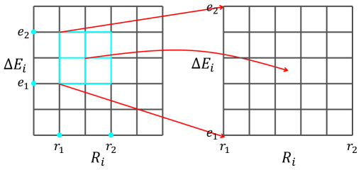
Figure 1: Schematic picture of iterative scanning

5 Results

fit type	$1+0$		$1+1$		$2+1$		$2+2$ (1st)		$2+2$ (2nd)
fit info	Prior	Result	Prior	Result	Prior	Result	Prior	Result	Prior	Result
$A_{0}$	none	0.0182(29)	0.018(14)	0.01724(52)	0.017(10)	0.01660(86)	0.017(10)	0.01724(35)	0.017(10)	0.01727(35)
$E_{0}$	none	2.0468(76)	2.05(11)	2.0448(22)	2.045(23)	2.0428(31)	2.043(23)	2.0449(18)	2.045(23)	2.0450(18)
$R_{1}$			none	3.5(58)	3.5(35)	0.755(82)	0.76(76)	0.646(84)	0.65(34)	0.639(79)
$\Delta E_{1}$			none	0.36(12)	0.36(36)	0.255(12)	0.26(26)	0.242(14)	0.24(11)	0.241(13)
$R_{2}$					none	0.93(37)	0.93(93)	1.879(76)	1.9(19)	1.888(75)
$\Delta E_{2}$					none	0.33(10)	0.33(33)	0.475(21)	0.48(48)	0.477(21)
$R_{3}$							none	2.10(49)	none	2.05(43)
$\Delta E_{3}$							none	0.58(15)	none	0.57(14)
fit range	$21\leq t\leq 29$		$13\leq t\leq 29$		$7\leq t\leq 29$		$3\leq t\leq 29$		$3\leq t\leq 29$

Table 5: Preliminary results from the sequential Bayesian fitting.

As explained in Subsection 4.2, we determine the initial guess for the 1+0 fit using the Newton method. The fitting results for the 1+0 fit are summarized in the first column of Table 5. In Fig. 2, we present results for the effective masses $m_{\text{eff}}^{(1)}$ and $m_{\text{eff}}^{(2)}$, where

$$m_{\text{eff}}^{(j)}(t) =\frac{1}{j}\ln\left(\frac{C(t)}{C(t+j)}\right)\,.$$ (21)

We set the fit range for the 1+0 fit to the region where the effective mass signal does not oscillate with respect to time. It corresponds to the magenta color in Fig. 2. We set up the Bayesian prior information (info) for 1+1 as follows.

$$A^{\text{p}}_{0} =A^{[1+0]}_{0}\pm[0.8\times A^{[1+0]}_{0}]$$ (22)

$$E^{\text{p}}_{0} =E^{[1+0]}_{0}\pm[14.53\times\sigma^{[1+0]}_{E_{0}}]$$ (23)

where the superscript ${}^{\text{p}}$ represent the prior info. Here, we take the maximum fluctuation of the effective masses within the 1+0 fit range as the prior width for $E_{0}$, which corresponds to the blue dashed line in Fig. 2.

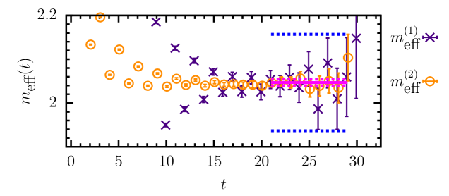
Figure 2: Effective masses for the 1+0 fit.

We set the fit range for the 1+1 fit to $13\leq t\leq 29$ so that it minimize the $\chi^{2}$/d.o.f with a given prior info. We also apply the same principle of the minimum $\chi^{2}$/d.o.f to find the optimal fit ranges for the 2+1 and 2+2 fits. In the 2+1 fit, we perform the stability test on $A_{0}$ and $E_{0}$ to find the optimal prior widths such that we find the minimum value which does not change the fit results for $A_{0}$ and $E_{0}$. In the 2+2 fit, we perform the same stability test on $R_{1}$ and $\Delta E_{1}$ to find the optimal prior widths. In the first 2+2 fit, the fit results for $R_{2}$ and $\Delta E_{2}$ shift from the prior info by about 1$\sigma$. Hence, we update the prior info for the second 2+2 fit to reflect on this shift.

At present we are working on the 3+2 and 2+3 fits to consume the entire time slices for the fit range $1\leq t\leq 29$.

6 Conclusion

We have multiple options to choose time slices when we apply the Newton method to obtain the initial guess. This provides a natural test to check whether the $\chi^{2}$ minimizer finds a local minimum or the global minimum. In addition, the Newton method reduces the number of iterations for the $\chi^{2}$ minimizer dramatically. At present, the results which we present here are preliminary, but good enough to insure that the Newton method is highly promising. Our final results will be available soon. Please stay tuned for our future report.

References

- [1] A. X. El-Khadra, A. S. Kronfeld, and P. B. Mackenzie Phys. Rev. D55 (1997) 3933–3957, [hep-lat/9604004].
- [2] M. B. Oktay and A. S. Kronfeld Phys. Rev. D78 (2008) 014504, [0803.0523].
- [3] LANL-SWME Collaboration, J. A. Bailey, Y.-C. Jang, S. Lee, W. Lee, and J. Leem Phys. Rev. D 105 (2022), no. 3 034509, [2001.05590].
- [4] J. A. Bailey, T. Bhattacharya, R. Gupta, Y.-C. Jang, W. Lee, J. Leem, S. Park, and B. Yoon EPJ Web Conf. 175 (2018) 13012, [1711.01786].
- [5] E. Follana, Q. Mason, C. Davies, K. Hornbostel, G. P. Lepage, J. Shigemitsu, H. Trottier, and K. Wong Phys. Rev. D75 (2007) 054502, [hep-lat/0610092].
- [6] B. Yoon et al. Phys. Rev. D93 (2016), no. 11 114506, [1602.07737].
- [7] A. Bazavov et al. Phys. Rev. D87 (2013), no. 5 054505, [1212.4768].
- [8] A. Bazavov et al. Phys. Rev. D85 (2012) 114506, [1112.3051].
- [9] C. G. Broyden IMA Journal of Applied Mathematics 6 (1970), no. 1 76–90.
- [10] R. Fletcher The Computer Journal 13 (1970), no. 3 317–322.
- [11] D. Goldfarb Mathematics of Computation 24 (1970), no. 109 23–26.
- [12] D. F. Shanno Mathematics of Computation 24 (1970), no. 111 647–656.
- [13] W. H. Press, S. A. Teukolsky, W. T. Vetterling, and B. P. Flannery, Numerical Recipes. Cambridge University Press, 3 ed., 2007. pages 477–483.
- [14] C. G. Broyden Mathematics of Computation 19 (1965), no. 92 577–593.