Nonlinear dynamics of an epidemic compartment model with asymptomatic infections and mitigation

Abstract

A significant proportion of the infections driving the current SARS-CoV-2 pandemic are transmitted asymptomatically. Here we introduce and study a simple epidemic model with separate compartments comprising asymptomatic and symptomatic infected individuals. The linear dynamics determining the outbreak condition of the model is equivalent to a renewal theory approach with exponential waiting time distributions. Exploiting a nontrivial conservation law of the full nonlinear dynamics, we derive analytic bounds on the peak number of infections in the absence and presence of mitigation through isolation and testing. The bounds are compared to numerical solutions of the differential equations.

1 Introduction

The ongoing SARS-CoV-2 pandemic highlights the importance of presymptomatic and asymptomatic infections [1, 2, 3, 4, 5, 6, 7, 8] and their effects on the ability to control outbreaks by non-pharmaceutical interventions [9, 10, 11, 12]. These effects are principally twofold. On the one hand, asymptomatic infections often remain undetected [13], which makes it difficult to monitor the spread of the disease in the population and confounds estimates of epidemiological parameters [14]. On the other hand, asymptomatic individuals do not require medical treatment and therefore do not contribute to the burden on the health care system caused by the epidemic.

A mathematical framework for modeling epidemics with asymptomatic infections based on renewal theory was developed by Fraser et al. in the context of the first SARS pandemic [15]. In this approach, the transmission of the disease is described by two functions $\beta(\tau)$ and $\sigma(\tau)$ that quantify the infectiousness of an indvidual and the probability for the individual to still be asymptomatic, respectively, as a function of the time $\tau$ since infection. Both functions can be estimated from empirical data [9, 12]. For a given set of functions $\beta,\sigma$ the theory provides a condition for an outbreak to occur, and quantifies the efficacy of isolation and contact tracing measures required for controlling it. As usual, the outbreak criterion is determined by the linear dynamics in the early stages of the epidemic. It takes the form $R_{0}>1$, where $R_{0}$ denotes the basic reproduction number defined as the expected number of secondary infections conferred by an infected individual in a fully susceptible population [16, 17, 18, 19].

However, in order to predict the severity of an outbreak, it is necessary to understand the nonlinear epidemic dynamics, which determines key quantities such as the total number of infections at the end of the outbreak [21, 22] or the number of infected individuals at the peak of the epidemic. The purpose of this contribution is to introduce and study a simple, analytically tractable model that allows to address the effect of asymptomatic infections on the full nonlinear time evolution of an epidemic. The model is a minimal extension of the standard SIR-model [16, 17, 18, 19, 20] that includes separate populations of asymptomatic and symptomatic infected individuals; similar models have been introduced previously and are sometimes referred to as SAIR models, see [23] and A.

The specific version of the SAIR model considered in this work is defined in the next section. In Sections 2.2 and 2.3 we analyze the linear dynamics and identify the basic reproduction number, the fraction of asymptomatic infections and the functions $\beta(\tau)$ and $\sigma(\tau)$. An extended model that includes the recovery of asymptomatic individuals will be discussed in Sect. 2.4. In Sect. 3 we make use of the nontrivial conservation law of the dynamical system to derive an analytic upper bound on the peak number of symptomatically infected individuals, which is compared to numerical solutions. Section 4 generalizes the model to include the effects of isolation (of symptomatic individuals) and testing (of asymptomatic individuals), and Section 5 summarizes our conclusions.

2 Epidemic dynamics with asymptomatic infections

2.1 Dynamical equations

We consider a population of constant size $N$ which is subdivided into compartments comprising susceptible ($S$), asymptomatically infected ($A$), symptomatically infected ($I$) and removed ($R$) individuals. For the sake of simplicity, asymptomatic and symptomatic individuals are taken to infect the susceptible individuals at the same rate $\lambda$. Moreover, following previous work [12, 15], we assume that all asymptomatic individuals develop symptoms and assign a rate $\xi$ to this process. We shall see below in Sec. 2.3 that the probability $\sigma(\tau)$ that an infected individual has not developed symptoms up to time $\tau$ may nevertheless remain nonzero for $\tau\to\infty$. Symptomatically infected individuals are transferred to the removed compartment (by recovery or death) at rate $\mu$. Denoting the number of individuals in the different compartments by $S(t)$, $A(t)$, $I(t)$ and $R(t)$, respectively, this leads to the following set of differential equations:

$$\dot{S}=-\frac{\lambda}{N}(A+I)S$$ (1)

$$\dot{A}=\frac{\lambda}{N}(A+I)S-\xi A$$ (2)

$$\dot{I}=\xi A-\mu I$$ (3)

$$\dot{R}=\mu I$$ (4)

These equations define a special case of a larger class of models with asymptomatic infections that are reviewed, e.g., in [24] and in A. Here we focus on the minimal version (1-4) that extends the SIR model by a single additional parameter, $\xi$, which is related to the fraction of asymptomatic infections (see Sect. 2.3). The SIR model is recovered in the limit $\xi\to\infty$. Figure 1 shows an exemplary numerical solution of the system (1-4).

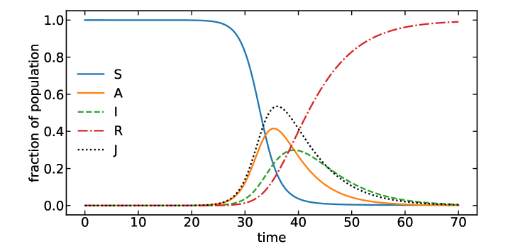
Figure 1: Illustration of the epidemic dynamics described by Eqs. (1-4). The figure shows the time courses of $S(t)$, $A(t)$, $I(t)$ and $R(t)$, as well as the auxiliary quantity $J(t)$ defined in Eq. (22), which peaks when $S=S^{\ast}=\frac{N}{R_{0}}$. Dimensionless parameters are $R_{0}=6$ and $\theta=0.5$, and the mean infection time is $\mathbb{E}(\tau)=10$. The initial condition consists of one asymptomatically infected individual in a population of size $N=10^{8}$.

2.2 Distribution of infection times

Let $q(\tau)$ denote the probability that an individual infected at time $t$ is still infectious at time $t+\tau$. An infectious individual is either asymptomatic or symptomatic, and the transitions $A\to I$ and $I\to R$ occur at rates $\xi$ and $\mu$, respectively. We can thus write $q(\tau)=q_{A}(\tau)+q_{I}(\tau)$, where the contributions $q_{A}$ and $q_{I}$ from asymptomatic and symptomatic individuals satisfy the linear system

$$\dot{q}_{A}=-\xi q_{A},\;\;\;\dot{q}_{I}=\xi q_{A}-\mu q_{I}.$$ (5)

These equations follow directly from Eqs. (2) and (3) by omitting the infection term in Eq. (2). The solution of (5) with initial conditions $q_{A}(0)=1,q_{I}(0)=0$ reads

$$q(\tau)=\frac{1}{\mu-\xi}\left(\mu e^{-\xi\tau}-\xi e^{-\mu\tau}\right),$$ (6)

and taking the derivative we obtain the distribution of infection times as

$$p(\tau)=-\frac{dq}{d\tau}=\frac{\mu\xi}{\mu-\xi}\left(e^{-\xi\tau}-e^{-\mu\tau}\right).$$ (7)

In the special case $\xi=\mu$ these expressions reduce to

$$q(\tau)=(1+\mu\tau)e^{-\mu\tau},\;\;\;\;p(\tau)=\mu^{2}\tau e^{-\mu\tau}.$$ (8)

It is instructive to interpret the distribution (7) stochastically. As noted by Leung et al. [22], compartment models formulated in terms of ordinary differential equations implicitly assume that the transitions between the different compartments occur according to Markov processes with exponentially distributed waiting times. For the two-step process $A\to I\to R$ described by the linear system (5) this implies that the total infection time can be written as a sum $\tau=t_{\xi}+t_{\mu}$ of two exponentially distributed waiting times $t_{\xi}$ and $t_{\mu}$ with parameters $\xi$ and $\mu$, which also leads to the probability density (7). In general, for models with multiple compartments of infected individuals, the distribution of infection times is given by a convolution of exponential functions [18, 25].

2.3 Basic reproduction number and fraction of asymptomatic infections

To set the stage, we briefly recall the approach of Fraser et al. [15]. Denoting by $\beta(\tau)$ the infection rate of an individual at time $\tau$ since they were infected, the basic reproducion number is given by

$$R_{0}=\int_{0}^{\infty}d\tau\,\beta(\tau),$$ (9)

and an outbreak occurs if $R_{0}>1$. Infectious individuals are asymptomatic at the time of infection, and remain in this state up to time $\tau$ with probability $\sigma(\tau)$. Accordingly, the fraction of asymptomatic infections is

$$\theta=\frac{\int_{0}^{\infty}d\tau\,\sigma(\tau)\beta(\tau)}{\int_{0}^{\infty}d\tau\,\beta(\tau)}=R_{0}^{-1}\int_{0}^{\infty}d\tau\,\sigma(\tau)\beta(\tau).$$ (10)

In the following we determine the functions $\beta(\tau)$ and $\sigma(\tau)$ for the model defined by the differential equations (1-4). The infectiousness function is given by $\beta(\tau)=\lambda q(\tau)$, and correspondingly the basic reproduction number is

$$R_{0}=\int_{0}^{\infty}d\tau\,\lambda q(\tau)=\lambda\mathbb{E}(\tau)=\lambda\left(\frac{1}{\xi}+\frac{1}{\mu}\right)=R_{0}^{A}+R_{0}^{I},$$ (11)

where $\mathbb{E}(\tau)$ is the expectation of the probability density (7) of infection times, and $R_{0}^{A}=\frac{\lambda}{\xi}$ and $R_{0}^{I}=\frac{\lambda}{\mu}$ denote the contributions of asymptomatic and symptomatic infections to $R_{0}$ [7, 9, 12, 24]. The fraction of asymptomatic infections is therefore

$$\theta=\frac{R_{0}^{A}}{R_{0}}=\frac{\mu}{\mu+\xi}.$$ (12)

Combining (11) and (12) we can write

$$R_{0}=\frac{R_{0}^{I}}{1-\theta},$$ (13)

which shows how the presence of (potentially undetected) asymptomatic infections increases the basic reproduction number beyond the value $R_{0}^{I}$ estimated from symptomatic infections only.

The second defining function of the theory of [15] is the probability for an infected individual to still be asymptomatic after time $\tau$, which can be obtained as

$$\sigma(\tau)=\frac{q_{A}(\tau)}{q(\tau)}=\frac{\mu-\xi}{\mu-\xi e^{-(\mu-\xi)\tau}}.$$ (14)

Interestingly, the function (14) displays a qualitative change of behaviour when $\mu=\xi$ or $\theta=\frac{1}{2}$. For $\theta<\frac{1}{2}$ the function approaches zero exponentially for large $\tau$, whereas for $\theta>\frac{1}{2}$ it attains a nonzero limiting value of $2-\frac{1}{\theta}>0$. Such a scenario was also discussed in [15]. Mathematically, it reflects the fact that, when $\mu>\xi$, for exceptionally large values of the total infection time $\tau=t_{\xi}+t_{\mu}$ it is likely that $t_{\xi}\gg t_{\mu}$. In the degenerate case $\xi=\mu$, $\sigma(\tau)$ decays algebraically as $(1+\mu\tau)^{-1}$. It is readily checked that inserting (14) into (10) reproduces the relation (12) for the fraction of asymptomatic infections.

Together the relations (11) and (12) specify the ratios of the three rates $(\lambda,\xi,\mu)$ defining the SAIR model. This implies that, up to an overall rescaling of time, the (linear and nonlinear) behavior of the dynamical system (1-4) is fully determined by the two dimensionless epidemiological parameters $R_{0}$ and $\theta$.

2.4 Asymptomatic recovery

In this section we assume that asymptomatically infected individuals recover at rate $\mu_{A}>0$ without previously developing symptoms. This changes Eqs. (2) and (4) into

$$\dot{A}=\frac{\lambda}{N}(A+I)S-(\xi+\mu_{A})A$$ (15)

$$\dot{R}=\mu I+\mu_{A}A.$$ (16)

The new rate $\mu_{A}$ can be expressed in terms of an additional dimensionless parameter $\vartheta$ defined as the fraction of individuals that never develop any symptoms. Since the development of symptoms and recovery are competing processes that both contribute to the loss of asymptomatic infected individuals, this fraction is given by the ratio

$$\vartheta=\frac{\mu_{A}}{\xi+\mu_{A}}.$$ (17)

Importantly, as we now show, this is generally distinct from the fraction $\theta$ of asymptomatic infections.

The computation of the epidemiological functions $q(\tau)$ and $\sigma(\tau)$ and of the parameters $R_{0}$ and $\theta$ proceeds along the lines of Sects. 2.2 and 2.3. Replacing the first equation in (5) by $\dot{q}_{A}=-(\xi+\mu_{A})q_{A}$, the probability $q(\tau)$ that an individual is still infectious at time $\tau$ becomes

$$q(\tau)=\frac{1}{\mu-\mu_{A}-\xi}\left[(\mu-\mu_{A})e^{-(\xi+\mu_{A})\tau}-\xi e^{-\mu\tau}\right].$$ (18)

Integrating this expression over $\tau$ we obtain

$$R_{0}=\frac{\lambda}{\mu}\left(\frac{\xi+\mu}{\xi+\mu_{A}}\right)=\lambda\left[\frac{1}{\xi+\mu_{A}}+(1-\vartheta)\frac{1}{\mu}\right]=R_{0}^{A}+R_{0}^{I}.$$ (19)

Similar to (11), the second equality expresses $R_{0}$ in terms of the expected infection times in the asymptomatic and the symptomatic compartment, which are given by $1/(\xi+\mu_{A})$ and $1/\mu$, respectively. Since not all individuals develop symptoms, the latter contribution is weighted by a factor $1-\vartheta$. As in Sect. 2.3, the fraction of asymptomatic infections is then obtained as

$$\theta=\frac{R_{0}^{A}}{R_{0}}=\frac{(\xi+\mu_{A})^{-1}}{(\xi+\mu_{A})^{-1}+(1-\vartheta)\mu^{-1}}=\frac{\mu}{\mu+\xi},$$ (20)

which, remarkably, does not depend on $\mu_{A}$. Based on Eqs.(17) and (20), we see that $\theta>\vartheta$ for $\mu>\mu_{A}$ and $\theta<\vartheta$ for $\mu<\mu_{A}$. Finally, the function $\sigma(\tau)$ is given by the expression

$$\sigma(\tau)=\frac{q_{A}(\tau)}{q(\tau)}=\frac{\mu-\mu_{A}-\xi}{\mu-\mu_{A}-\xi e^{-(\mu-\mu_{A}-\xi)\tau}},$$ (21)

which approaches a positive limiting value for $\tau\to\infty$ when $\mu>\mu_{A}+\xi$.

The model simplifies considerably when symptomatic and asymptomatic individuals recover at the same rate. In that case the functions $q(\tau)$ and $\sigma(\tau)$ become pure exponentials, $\theta=\vartheta$, and $R_{0}=\lambda/\mu$ independent of $\xi$. In fact, as pointed out in [23], for $\mu=\mu_{A}$ the total number of infected individuals $A+I$ satisfies standard SIR dynamics, and the transfer between the two compartments has no consequences for the devlopment of the epidemic. We will return to this case below in Sect. 3.

3 Peak of the epidemic

In the following we focus on the peak number of symptomatic infections $I_{\mathrm{max}}$ as a measure for the severity of an outbreak. In this section we derive a rigorous upper bound on $I_{\mathrm{max}}$. Upper bounds are of particular significance for the evaluation of worst case scenarios.

The key step in the analysis is the identification of a nontrivial conservation law for the dynamical system defined by Eqs.(1,2,3,4). For this purpose we introduce the auxiliary quantity

$$J(t)=A(t)+\phi I(t).$$ (22)

Using (2) and (3), we see that with the choice

$$\phi=\frac{\xi}{\xi+\mu}=1-\theta$$ (23)

$J(t)$ satisfies

$$\dot{J}=\dot{A}+\phi\dot{I}=\frac{\lambda}{N}(S-S^{\ast})(A+I)$$ (24)

where $S^{\ast}=\frac{N}{R_{0}}$. Thus $J(t)$ attains its peak value $J_{\mathrm{max}}$ at a time $t_{J}$ defined by $S(t_{J})=S^{\ast}$. Dividing Eq. (24) by Eq. (1) we obtain $\frac{dJ}{dS}=\frac{S^{\ast}}{S}-1$, which can be integrated to yield $J-J_{0}=S^{\ast}\ln\left(\frac{S^{\ast}}{S_{0}}\right)+S_{0}-S$. Rearranging terms we conclude that the quantity

$$H\equiv J+S-S^{\ast}\ln S=A+S+(1-\theta)I-\frac{N}{R_{0}}\ln S$$ (25)

is conserved under the dynamics.

At the time $t_{I}$ at which $I(t)$ attains its maximum value $I_{\mathrm{max}}$ we have $\dot{I}=0$ and therefore

$${\color[rgb]{0,0,0}{A(t_{I})=\frac{\mu}{\xi}I(t_{I}),}}$$ (26)

which implies that

$$H(t_{I})=\psi I_{\mathrm{max}}+\tilde{S}-S^{\ast}\ln\tilde{S}.$$ (27)

Here $\tilde{S}=S(t_{I})$ and

$$\psi=\phi+\frac{\mu}{\xi}=1-\theta+\frac{\theta}{1-\theta}\geq 1.$$ (28)

Equating (27) to the initial value $H(0)=N-S^{\ast}\ln N$ of $H$ corresponding to a completely susceptible population, we conclude that

$$I_{\textrm{max}}=\frac{1}{\psi}\left[N-\tilde{S}+S^{\ast}\ln\left(\frac{\tilde{S}}{N}\right)\right].$$ (29)

Observing finally that the quantity in square brackets on the right hand side of (29) is maximized by $\tilde{S}=S^{\ast}$, we arrive at the bound

$$I_{\textrm{max}}\leq\frac{1}{\psi}J_{\textrm{max}}=\frac{N}{\psi}\left(1-\frac{1}{R_{0}}(1+\ln R_{0})\right).$$ (30)

Figure 2 illustrates the dependence of the bound (30) on the fraction of asymptomatic infections for two scenarios, where either the total basic reproduction number $R_{0}$, or the reproduction number due to symptomatic infections, $R_{0}^{I}$, is kept constant. In the first case $I_{\mathrm{max}}$ decreases monotonically with $\theta$, but the decrease is less than simply by a factor of $1-\theta$, as one might have naively expected. In particular, for small $\theta$ the decrease is quadratic rather than linear in $\theta$. Under the condition of constant $R_{0}^{I}$ the total basic reproduction number increases with increasing $\theta$ and diverges for $\theta\to 1$, see Eq. (13). In this case the bound displays a maximum at an intermediate value of $\theta$ but nevertheless tends to zero for $\theta\to 1$. The figure also shows exact results for $I_{\mathrm{max}}$ obtained by numerically integrating the system (1-4). The analytic bound is seen to predict the qualitative behavior of $I_{\mathrm{max}}$ very well, but there are significant quantitative deviations for large $R_{0}$ and intermediate values of $\theta$.

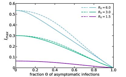
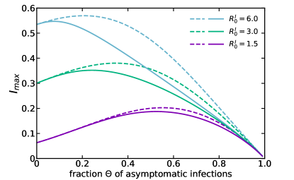
Figure 2: The peak number of symptomatic cases $I_{\mathrm{max}}$ as a function of the fraction $\theta$ of asymptomatic infections. Dashed lines show the analytic bound (30) and full lines show the results of the numerical solution of the dynamical system. In the left panel the total basic reproduction number $R_{0}$ is kept constant at the values $R_{0}=6$, 3 and 1.5 (from top to bottom). The right panel shows the corresponding behavior at constant $R_{0}^{I}=6$, 3 and 1.5. In the latter case the total basic reproduction number increases with the fraction of asymptomatic infections according to Eq. (13).

A similar bound can be derived for the model with asymptomatic recovery considered in Sect. 2.4. For convenience we restrict ourselves to the special case of equal recovery rates for symptomatic and asymptomatic individuals, $\mu=\mu_{A}$. Then the total number of infected individuals $A+I$ follows standard SIR dynamics, and its exact peak value $(A+I)_{\textrm{max}}$ is known [16]. Using again the relation (26) and the fact that

$$A(t_{I})+I(t_{I})\leq(A+I)_{\textrm{max}}=N\left(1-\frac{1}{R_{0}}(1+\ln R_{0})\right),$$ (31)

we arrive at the bound

$$I_{\textrm{max}}\leq(1-\theta)N\left(1-\frac{1}{R_{0}}(1+\ln R_{0})\right).$$ (32)

Since $1/\psi\geq 1-\theta$ for $\theta\in[0,1]$, for a given value of $R_{0}$ the right hand side of (32) is always smaller than that of (30).

4 SAIR model with mitigation

4.1 Dynamical equations with isolation and testing

The isolation of symptomatic cases and the testing of asymptomatic individuals are among the most important strategies for containing an epidemic by non-pharmaceutical means [9, 11, 12, 15, 26, 27]. Adding the corresponding processes to the dynamical system (1-4) with isolation and testing rates $\nu_{I}$ and $\nu_{T}$ leads to the extended model

$$\dot{S}=-\frac{\lambda}{N}(A+I)S$$ (33)

$$\dot{A}=\frac{\lambda}{N}(A+I)S-(\xi+\nu_{T})A$$ (34)

$$\dot{I}=\xi A-(\mu+\nu_{I})I$$ (35)

$$\dot{T}=\nu_{T}A-\xi T$$ (36)

$$\dot{Q}=\nu_{I}I+\xi T-\mu Q$$ (37)

$$\dot{R}=\mu(I+Q),$$ (38)

where the added compartments comprise asymptomatic cases that have been tested positively ($T$) and isolated (quarantined) symptomatic cases ($Q$), respectively. Positively tested individuals develop symptoms at rate $\xi$ and isolated individuals are removed at rate $\mu$. Since testing competes with the development of symptoms and isolation competes with removal, the efficacy of the two interventions can be quantified by the ratios

$$\epsilon_{T}=\frac{\nu_{T}}{\nu_{T}+\xi},\;\;\;\;\epsilon_{I}=\frac{\nu_{I}}{\nu_{I}+\mu}.$$ (39)

To be precise, $\epsilon_{T}$ is the fraction of asymptomatic cases that are detected before developing symptoms, and $\epsilon_{I}$ is the fraction of symptomatic cases that are isolated before being removed. Repeating the analysis of Sections 2.2 and 2.3 for the model with mitigation we arrive at the expression

$$\tilde{R}_{0}=\lambda\frac{\xi+\mu+\nu_{I}}{(\xi+\nu_{T})(\mu+\nu_{I})}=(1-\epsilon_{T})[1-\epsilon_{I}(1-\theta)]R_{0}$$ (40)

for the basic reproduction number in the presence of mitigation. For $\epsilon_{T}=0$ this reproduces a result of [15], who define an outbreak to be controlled by the intervention if $\tilde{R}_{0}\leq 1$. Figure 3 delineates the region of controlled outbreaks in the $(\epsilon_{I},\epsilon_{T})$-plane for $\theta=\frac{1}{3}$ and different values of $R_{0}$.

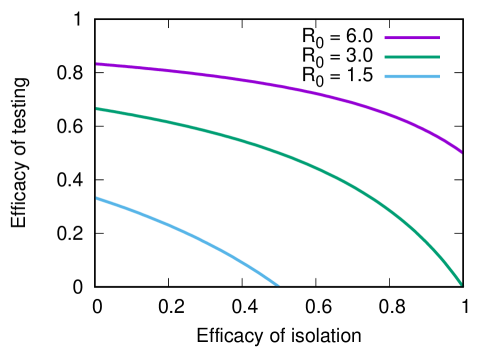
Figure 3: The efficacy of testing $\epsilon_{T}$ required to reach the condition $\tilde{R}_{0}=1$ of controlling the outbreak is shown as a function of the efficacy of isolation $\epsilon_{I}$. The fraction of asymptomatic infections is $\theta=1/3$, and the total basic reproduction number is $R_{0}=6$, 3 and 1.5 (from top to bottom). Points above the respective lines correspond to successful mitigation that is sufficient to control the outbreak.

4.2 Peak number of symptomatic cases

Since symptomatic individuals require medical care irrespective of whether they have been isolated or not, the relevant measure for the severity of an outbreak in the presence of mitigation is the peak in the total number of symptomatic cases, i.e. the maximum $M_{\mathrm{max}}$ of $M(t)=I(t)+Q(t)$. To derive an upper bound on this quantity, we again make use of the auxiliary quantity $J(t)$ defined in (22), where the factor $\phi$ is now given by

$$\phi=\frac{\xi+\nu_{T}}{\xi+\mu+\nu_{I}}=\frac{1}{(1-\epsilon_{T})\left(1+\frac{\theta}{(1-\theta)(1-\epsilon_{I})}\right)}.$$ (41)

Analogous to Sect. 3 it can be shown that, for $\tilde{R}_{0}>1$, $J(t)$ attains its maximum when the number of susceptible individuals reaches $S^{\ast}=\frac{N}{\tilde{R}_{0}}$, and the maximum value $J_{\mathrm{max}}$ is given by the expression in Eq. (30) with $R_{0}$ replaced by $\tilde{R}_{0}$.

In the following we specialize to the case without testing ($\nu_{T}=0$). Then $T=0$, and Eqs. (35,37) can be combined to $\dot{M}=\xi A-\mu M$. At the time $t_{M}$ when $M$ reaches its maximum value we have $\dot{M}=0$ and therefore

$$M_{\mathrm{max}}=M(t_{M})=\frac{\xi}{\mu}A(t_{M})=\frac{1-\theta}{\theta}A(t_{M})\leq\frac{1-\theta}{\theta}J(t_{M})\leq$$

$$\leq\frac{1-\theta}{\theta}J_{\mathrm{max}}=\frac{1-\theta}{\theta}N\left(1-\frac{1}{\tilde{R}_{0}}(1+\ln\tilde{R}_{0})\right),$$ (42)

with $\tilde{R}_{0}=R_{0}(1-\epsilon_{I}(1-\theta))$ for $\epsilon_{T}=0$.

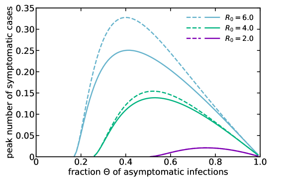
Figure 4: Peak value of the number of symptomatic cases for the SAIR model with perfect isolation ($\epsilon_{I}=1$) and no testing ($\epsilon_{T}=0$). In this limit all symptomatic cases belong to the quarantine compartment. The effective basic reproduction number is $\tilde{R}_{0}=\theta R_{0}$ and the outbreak is suppressed for $\theta<\frac{1}{R_{0}}$. Dashed lines show the analytic bound (4.2) and full lines show the results of the numerical solution of the dynamical system.

Bounding $A$ by $J$ in (4.2) is clearly a crude approximation when $\phi$ is not small. The bound is therefore expected to be most accurate when isolation is close to perfect, i.e. for $\epsilon_{I}\to 1$ or $\nu_{I}\to\infty$. In this limit symptomatically infected individuals are instantly transferred to the quarantine compartment, which implies that the terms proportional to $I$ can be removed from Eqs. (33,34) and Eq. (35) can be eliminated by replacing the term $\nu_{I}I$ in Eq. (37) by $\xi A$. Thus the limiting dynamics for perfect isolation and no testing reads

$$\dot{S}=-\frac{\lambda}{N}AS$$ (43)

$$\dot{A}=\frac{\lambda}{N}AS-\xi A$$ (44)

$$\dot{Q}=\xi A-\mu Q$$ (45)

$$\dot{R}=\mu Q.$$ (46)

Figure 4 compares the bound (4.2) to the peak value $M_{\mathrm{max}}=Q_{\mathrm{max}}$ obtained by numerically integrating the system (43-46). The agreement between the analytic and numerical results in this figure is similar to Fig. 2.

5 Conclusions

In this article we have introduced and studied a minimal compartment model that allows to investigate the effects of asymptomatic infections on the dynamics of an epidemic outbreak. The time evolution of the model is fully specified by two dimensionless parameters, the basic reproduction number $R_{0}$ and the fraction of asymptomatic infections $\theta$. Empirical estimates of $\theta$ for SARS-CoV-2 vary widely [3, 4], but it is undisputed that asymptomatic infections play a significant role in the current pandemic [8]; a recent meta-analysis concluded that $\theta\geq\frac{1}{3}$ [5].

Our approach is complementary to previous work based on renewal theory, which determines the conditions for an outbreak from the distributions of the times during which individuals are infectious and/or symptomatic [9, 12, 15, 19]. Whereas the structure of our model constrains these distributions to be of exponential form (Sect. 2.2), it also enables us to go beyond the initial stages of the outbreak and describe the full nonlinear dynamics. Mitigation strategies such as testing and isolation that differentiate between asymptomatic and symptomatic cases can be incorporated in a straightforward way (Sect. 4), and the effects of additional processes such as asymptomatic recovery can be evaluated systematically (Sect. 2.4). Despite the highly simplified and sketchy character of our mathematical framework [20], the explicit analytic expressions that we have derived may help to parametrize and interpret data-driven studies of more complex models with predictive capabilities [9, 11, 12].

A common property of epidemic compartment models that often makes them analytically tractable is the existence of nontrivial conservation laws [16], which is linked to an underlying Hamiltonian structure [28, 29, 30]. This feature provides a formal connection between mathematical epidemiology and theoretical physics. Here we exploit such a conservation law to derive rigorous analytic bounds on the peak number of symptomatic infections $I_{\mathrm{max}}$, which serves as measure for the severity of an outbreak and its societal consequences. Remarkably, under two scenarios illustrated in Figs. 2 and 4 we find that the peak number of infections varies non-monotonically with $\theta$. This reflects the dual role of asymptomatic cases: Although they increase the severity of the outbreak by increasing the basic reproduction number $R_{0}$, they do not contribute to the disease burden. While it may seem obvious that $I_{\mathrm{max}}=0$ for a fully asymptomatic (‘silent’) epidemic ($\theta=1$), the proof that this remains true even if $R_{0}$ diverges in the limit $\theta\to 1$ requires the explicit mathematical analysis carried out in Sect. 3.

The SARS-CoV-2 virus has undergone significant evolution over the past two years, and the concomitant changes in epidemiological parameters have contributed to the difficulty of controlling the pandemic [8]. The observed increase of the basic reproduction number $R_{0}$ with each newly emerging variant was to be expected on evolutionary grounds, but the selective forces acting on viral life history traits such as the time of the onset of symptoms or the severity of the disease are complex and not well understood. Theoretical work addressing this question makes use of SAIR-type models that are coupled to the evolutionary dynamics of the pathogen population [31, 32]. As such, a better analytic understanding of these models may contribute to forecasting the time course of future pandemics.

Appendix A SAIR models

Epidemic compartment models with asymptomatic infections go back at least to the work of Kemper in 1978 [33]. One may broadly distinguish between models that allow for a loss of immunity, and hence the approach to an endemic state, by including a transfer from the removed to the susceptible compartment [31, 33, 34, 35], and those that assume irreversible immunization [7, 23, 27, 32, 36, 37]. To position our contribution within the latter body of work, it is useful to consider the following generalization of the model defined by Eqs. (1-4):

$$\dot{S}=-\frac{\lambda}{N}(\delta_{A}A+\delta_{I}I)S$$ (47)

$$\dot{A}=(1-\eta)\frac{\lambda}{N}(\delta_{A}A+\delta_{I}I)S-(\xi+\mu_{A})A$$ (48)

$$\dot{I}=\eta\frac{\lambda}{N}(\delta_{A}A+\delta_{I}I)S+\xi A-\mu I$$ (49)

$$\dot{R}=\mu I+\mu_{A}A$$ (50)

Here the parameters $\delta_{A},\delta_{I}\in[0,1]$ quantify the relative infectiousness of indidivuals in the compartments $A$ and $I$, $\eta\in[0,1]$ is the probability that an infected individual develops symptoms immediately after infection, and $\mu_{A}\geq 0$ is the rate at which $A$-individuals are removed without developing symptoms. The basic SAIR-model of Sect. 2.1 is recovered for $\delta_{A}=\delta_{I}=1$ and $\eta=\mu_{A}=0$.

The dynamical system (47-50) includes several special cases that have been considered previously in the literature.

• For $\eta=\delta_{A}=\mu_{A}=0$ the model reduces to the well-known SEIR-model, where the $A$-compartment (in this case denoted by $E$) contains exposed individuals that are infected but not infectious [17, 38].

• Ansumali et al. [23] considered the model with $\eta=0,\delta_{A}=\delta_{I}=1,\mu_{A}=\mu$, which is a special case of the model with asymptomatic recovery considered in Sect. 2.4.

• Dobrovolny [7] studied the model with $\xi=0$ and used it to analyze data from the SARS-Cov-2 epidemics in several states of the USA.

• For $\delta_{A}=1,\delta_{I}=\eta=\mu_{A}=0$ the model reduces to the SAIR-model with perfect isolation of symptomatic individuals that is considered in Sect. 4.2. In this case the $Q$-compartment of quarantined individuals plays the role of the $I$-compartment in Eqs. (47-50).

References

References

- [1] C. Rothe et al., Transmission of 2019-nCoV Infection from an Asymptomatic Contact in Germany. N. Engl. J. Med. 382:970–971 (2020)
- [2] L.-S. Huang, L. Li, L. Dunn and M. He, Taking account of asymptomatic infections: A modeling study of the COVID-19 outbreak on the Diamond Princess cruise ship. PLoS ONE 16:e0248273 (2021)
- [3] O. Byambasuren, M. Cardona, K. Bell, J. Clark, M.-L. McLaws and P. Glasziou, Estimating the extent of asymptomatic COVID-19 and its potential for community transmission: Systematic review and meta-analysis. Official Journal of the Association of Medical Microbiology and Infectious Disease Canada 5:223-234 (2020)
- [4] M. Alene, L. Yismaw, M. A. Assemie, D. B. Ketema, B. Mengist, B. Kassie and T. Y. Birhan, Magnitude of asymptomatic COVID-19 cases throughout the course of infection: A systematic review and meta-analysis. PLoS ONE 16:e0249090 (2021)
- [5] D.P. Oran and E.J. Topol, The Proportion of SARS-CoV-2 Infections That Are Asymptomatic: A Systematic Review. Annals of Internal Medicine 174:655–662 (2021)
- [6] E.A. Meyerowitz, A. Richterman, I.I. Bogoch, N. Low and M. Cevik, Towards an accurate and systematic characterisation of persistently asymptomatic infection with SARS-CoV-2. Lancet Infect. Dis. 21:e163–e169 (2021)
- [7] H.M. Dobrovolny, Modeling the role of asymptomatics in infection spread with application to SARS-CoV-2. PLoS ONE 15:e0236976 (2020)
- [8] K. Koelle, M.A. Martin, R. Antia, B. Lopman and N.E. Dean, The changing epidemiology of SARS-CoV-2. Science 375:1116–1121 (2022)
- [9] L. Ferretti, C. Wymant, M. Kendall, L. Zhao, A. Nurtay, L. Abeler-Dörner, M. Parker, D. Bonsall and C. Fraser, Quantifying SARS-CoV-2 transmission suggests epidemic control with digital contact tracing. Science 368:eabb6936 (2020)
- [10] W.S. Hart, P.K. Maini and R.N. Thompson, High infectiousness immediately before COVID-19 symptom onset highlights the importance of continued contact tracing. eLife 10:e65534 (2021)
- [11] S. Contreras, J. Dehning, M. Loidolt, J. Zierenberg, F.P. Spitzner, J.H. Urrea-Quintero, S.B. Mohr, M. Wilczek, M. Wibral and V. Priesemann, The challenges of containing SARS-CoV-2 via test-trace-and-isolate. Nature Communications 12:378 (2021)
- [12] L. Tian et al., Harnessing peak transmission around symptom onset for non-pharmaceutical intervention and containment of the COVID-19 pandemic. Nature Communications 12:1147 (2021)
- [13] R. Li, S. Pei, B. Chen, Y. Song, T. Zhang, W. Yang and J. Shaman, Substantial undocumented infection facilitates the rapid dissemination of novel coronavirus (SARS-CoV-2). Science 368:489–493 (2020)
- [14] S.W. Park, D.M. Cornforth, J. Dushoff and J.S. Weitz, The time scale of asymptomatic transmission affects estimates of epidemic potential in the COVID-19 outbreak. Epidemics 31:100392 (2020)
- [15] C. Fraser, S. Riley, R.M. Anderson and N.M. Ferguson, Factors that make an infectious disease outbreak controllable. Proc. Natl. Acad. Sci. USA 101:6146 (2004)
- [16] J.D. Murray, Mathematical Biology I: An Introduction (Springer, New York 2002)
- [17] H.W. Hethcote, The Mathematics of Infectious Diseases. SIAM Review 42:599-653 (2000)
- [18] M.J. Keeling and P. Rohani, Modeling Infectious Diseases in Humans and Animals (Princeton University Press, 2008)
- [19] N.C. Grassly and C. Fraser, Mathematical models of infectious disease transmission. Nature Reviews Microbiology 6:477 (2008)
- [20] A. Traulsen, C.S. Gokhale, S. Shah and H. Uecker, The Covid-19 Pandemic: Basic Insights from Basic Mathematical Models. NAL-live 2022.3, 01000 (2022)
- [21] J. Ma and D.J.D. Earn, Generality of the Final Size Formula for an Epidemic of a Newly Invading Infectious Disease. Bulletin of Mathematical Biology 68:679 (2006)
- [22] K.Y. Leung, P. Trapman and T. Britton, Who is the infector? Epidemic models with symptomatic and asymptomatic cases. Mathematical Biosciences 301:190-198 (2018)
- [23] S. Ansumali, S. Kaushal, A. Kumar, M.K. Prakash and M. Vidyasagar, Modelling a pandemic with asymptomatic patients, impact of lockdown and herd immunity, with applications to SARS-CoV-2. Annual Reviews in Control 50:432–447 (2020)
- [24] R.H. Chisholm, P.T. Campbell, Y. Wu, S.Y.C. Tong, J. McVernon and N. Geard, Implications of asymptomatic carriers for infectious disease transmission and control. R. Soc. open sci. 5:172341 (2018)
- [25] A. Vazquez, Exact solution of infection dynamics with gamma distribution of generation intervals. Phys. Rev. E 103:042306 (2021)
- [26] K.I. Mazzitello, Y. Jiang and C.M. Arizmendi, Optimising SARS-CoV-2 pooled testing strategies on social networks for low-resource settings. J. Phys. A 54:294002 (2021)
- [27] R.I. Mukhamadiarov, S. Deng, S.R. Serrao, Priyanka, L.M. Childs and U.C. Täuber, Requirements for the containment of COVID-19 disease outbreaks through periodic testing, isolation, and quarantine. J. Phys. A 55:034001 (2022)
- [28] Y. Nutku, Bi-Hamiltonian structure of the Kermack-McKendrick model for epidemics. J. Phys. A 23:L1145 (1990)
- [29] A. Ballesteros, A. Blasco and I. Gutierrez-Sagredo, Hamiltonian structure of compartmental epidemiological models. Physica D 413:132656 (2020)
- [30] F. Haas, M. Kröger and R. Schlickeiser, Multi-Hamiltonian structure of the epidemics model accounting for vaccinations and a suitable test for the accuracy of its numerical solvers. J. Phys. A 55:225206 (2022).
- [31] C.M. Saad-Roy, N.S. Wingreen, S.A. Levin and B.T. Grenfell, Dynamics in a simple evolutionary-epidemiological model for the evolution of an initial asymptomatic infection stage. Proc. Natl. Acad. Sci. USA 117:11541–11550 (2020)
- [32] T. Day, S. Gandon, S. Lion and S.P. Otto, On the evolutionary epidemiology of SARS-CoV-2. Current Biology 30:R841–R870 (2020)
- [33] J.T. Kemper, The effects of asymptomatic attacks on the spread of infectious disease: A deterministic model. Bull. Math. Biol. 40:707–718 (1978)
- [34] M. Robinson and N.I. Stilianakis, A model for the emergence of drug resistance in the presence of asymptomatic infections. Math. Biosciences 243:163–177 (2013)
- [35] S. Ottaviano, M. Sensi and S. Sottile, Global stability of SAIRS epidemic models. Nonlinear Analysis: Real World Applications 65:103501 (2022)
- [36] F. Débarre, S. Bonhoeffer and R.R. Regoes, The effect of population structure on the emergence of drug resistance during influenza pandemics. J. R. Soc. Interface 4:893–906 (2007)
- [37] Z. Chladná, J. Kopfová, D. Rachinskii and P. Štepánek, Effect of Quarantine Strategies in a Compartmental Model with Asymptomatic Groups. J. Dyn. Diff. Equat. online first (2021)
- [38] S.J. Weinstein, M.S. Holland, K.E. Rogers and N.S. Barlow, Analytic solution of the SEIR epidemic model via asymptotic approximant. Physica D 411:132633 (2020)