A Study on the X-ray pulse profile and spectrum of the Crab pulsar
using NICER and Insight-HXMT’s Observations

Abstract

We analyze the energy dependence of the X-ray pulse profile and the phase-resolved spectra (PRS) of the Crab pulsar using observations from the Neutron star Interior Composition Explorer (NICER) and the Hard X-ray Modulation Telescope (Insight-HXMT). We parameterize the pulse profiles and quantify the evolution of these parameters in a broad energy band of 0.4-250 keV. A log-parabola function is used to fit the PRS in 2-250 keV, and the curvature of the spectrum, i.e., the evolution of photon index with energy, as represented by the parameter $\beta$ of the log-parabola model also changes with phase. The relation of $\beta$ and phase have two turning points slightly later than those of the pulse intensity profile, where the values of the $\beta$ are the lowest, suggesting that the energy loss rate of the particles are the lowest in the corresponding regions. A three-segment broken power-law model is also used to fit those PRS. The differences between the hard spectral index and the soft ones have distribution similar to that of $\beta$, confirming the fitting results of the log-parabola model, while the broken energies are generally higher in the region bridging the two pulses. We find anti-correlations between the spectral indices and curvature of the log-parabola model fitting and similar anti-correlation between the spectral indices and broken energies of the broken power law model fitting, suggesting a scenario that the highest energy particles are produced in regions where the radiation energy loss is also the strongest.

1 Introduction

The Crab pulsar (PSR B0531+21) is one of the most frequently studied objects in X-ray astrophysics. It has a period of about 33 ms, a spin down rate of $\dot{P}=4.2\times 10^{-13}$ s s^-1 and an energy loss power of $\dot{E}=5\times 10^{38}$ erg s^-1. Although observational data on this source have been gathered for about 50 years, the physics involved in this pulsar has not yet been completely understood. The position and size of the radiation regions, the distribution of secondary pairs, the magnetic field, the inclination and viewing angles, etc., together determine the pulse profiles and spectra in different energy bands (Cheng et al., 1986a, b). Studying the pulse profile and spectrum variations will thus help to explore the links between the multi-wavelength radiation properties and the physical conditions on this pulsar.

The pulse profiles of the Crab pulsar at all wavelengths are dominated by two pulses, separated by about 0.4 pulse phase. Previous studies show that the exact pulse morphology varies as a function of photon energy (Eikenberry & Fazio, 1997; Kuiper et al., 2001; Ge et al., 2012; Tuo et al., 2019): the intensities of both the second pulse and the bridge emission increase with energy relative to that of the first pulse in X-ray and followed by a downward trend above 1 MeV (Kuiper et al., 2001). However, some of these studies were either done in narrow energy bands that can not give quantitative results (Eikenberry & Fazio, 1997; Tuo et al., 2019), or incomplete for only adopting the flux ratio of the two pulses to describe the evolution of the pulse profile (Kuiper et al., 2001).

Actually the information contained in the energy dependence of the pulse profile can be revealed in more detail by phase resolved X-ray spectroscopy. The overall X-ray spectrum of the Crab pulsar could be well described by a power-law function and its spectral index varies with energy (Massaro et al., 2000; Weisskopf et al., 2004; Mineo et al., 2006). The phase-averaged total spectrum of the Crab nebula and pulsar in 1-100 keV has a photon index $\Gamma\sim 2.1$ (RXTE, BeppoSAX, EXOSAT, INTEGRAL/JEM X, Kirsch et al. (2005)), and a softer index of $\sim 2.20-2.25$ above 100 keV (INTEGRAL/SPI/ISGRI, CGRO Mineo et al. (2006); Kuiper et al. (2001)). The pulsed spectrum has a more complex evolution (Kuiper et al., 2001) and the photon index is about 1.6 in 0.3-3.8 keV (Weisskopf et al., 2011), 1.81 in 5-60 keV, 1.91 in 15-250 keV, and 1.96 in 0.1-300 GeV (Yan et al., 2018). For the phase-resolved X-ray spectra, Pravdo et al. (1997) found a phase evolution of the spectral index across the X-ray pulse in a reverse $S$ shape in 5-200 keV, i.e., the spectral index increases until the peak of the first pulse and then falls off, while the spectral index keeps increasing from the leading wing to the trail wing of the second pulse. Such a phase evolution trend holds albeit with different values in 0.3-3.8 keV (Weisskopf et al., 2011), 1-10 keV (Vivekanand, 2021), 3-60 keV (Ge et al., 2012), 3-78 keV (Madsen et al., 2015), 11-250 keV (Tuo et al., 2019), 15-500keV (Li et al., 2019), 20-500 keV (Mineo et al., 2006) and $>$ 100MeV (Abdo et al., 2010).

A three-dimensional outer magnetospheric gap model was proposed to explain the pulse profile, phase-resolved spectra, and polarization of the Crab pulsar (Cheng et al., 2000; Takata et al., 2007; Tang et al., 2008). Specifically, in the model of Cheng et al. (2000), the X-ray photons at different phases are produced by the radiations from different height range of regions in the magnetosphere. Recently, particle-in-cell (PIC) simulations are developed to study the pulsar magnetosphere that is more complex than a simple dipole (Philippov & Spitkovsky, 2014; Philippov et al., 2015a, b). Such PIC methods can therefore produce more complicated pulse profiles and have been successfully applied to the interpretation of Fermi observations of pulsars (Cerutti et al., 2016; Philippov & Spitkovsky, 2018). As the X-ray spectrum reflects the energy distribution and radiation cooling of the high energy electrons, phase-resolved spectroscopy in a broad X-ray band can provide information for theoretical studies on the high energy particle production and cooling, as well as the magnetic field geometry of the pulsar magnetosphere.

In this work, we use observations from the Neutron star Interior Composition Explorer (NICER) and the Hard X-ray Modulation Telescope (Insight-HXMT) to analyse the pulse morphology and phase-resolved spectra (PRS) for the Crab pulsar, providing further constraints on models of pulsar X-ray emission. The organization of this paper is as follows: data processing and reduction are presented in Section 2, analysis methods in Section 3, results in Section 4, discussions on the physical implications of our results and a summary in Section 5 and Section 6, respectively. Throughout the paper, errors of the parameters are at the one standard deviation level.

2 Observations and Data Reductions

2.1 Timing Ephemeris from Jodrell Bank Observatory

A 13 m radio telescope at Jodrell Bank Observatory monitors the Crab pulsar daily (Lyne et al., 1993), offering a radio ephemeris (denoted as JBE) that is used for the analyses of NICER and Insight-HXMT data. For monthly validity intervals, this ephemeris contains up-to-date parameters of the rotation frequency and its first two time derivatives. The database is available through the World Wide Web (http://www.jb.man.ac.uk/pulsar/crab.html). These JBE parameters, the pulsar coordinate R.A.=$83^{\circ}.63322$, decl.=$22^{\circ}.01446$(J2000) (Abdo et al., 2010), and solar system ephemeris JPL DE200 are used in this work.

2.2 NICER Observations and Data Reductions

The NICER is an International Space Station payload devoted to the study of neutron stars through soft X-ray timing in 0.2-12 keV. Its X-ray Timing Instrument (XTI) is an aligned collection of 56 X-ray concentrator optics (XRC) and silicon drift detector (SDD) pairs. Each XRC collects X-rays over a large geometric area from a roughly 30 arcmin² region of the sky and focuses them onto a small SDD. The SDD detects individual photons, recording their energies with good spectral resolution and their detection times to a $\sim$100 nanoseconds RMS relative to Universal Time (Prigozhin et al., 2016).

The NICER’s observations used in this paper are from 2017 August 25 to 2019 November 26, but only those with available JBE are used, and the total exposure time is about 339 ks. The data reduction is carried out by using NICERDAS software version 7a included in HEAsoft version 6.27.2, with calibration database version 20200722. Standard calibration processes as well as filtering to an entire NICER observation are performed by the command nicerl2. The cleaned photon events produced by the previous step are corrected to the solar system barycenter (SSB) and then used to fold pulse profiles in different soft X-ray energy bands. The cleaned events after corrected to SSB are also used to get the phase resolved spectrum. We extract the source spectrum with HEASoft XSELECT package (V.2.4e).

2.3 Insight-HXMT Observations and Data Reductions

The Insight-HXMT is China’s first X-ray astronomy satellite. It has three main payloads: the High Energy X-ray telescope (HE, $20-350\,\rm{keV}$, $5100\,\rm{cm}^{2}$), the Medium Energy X-ray telescope (ME, $8-35\,\rm{keV}$, $952\,\rm{cm}^{2}$) and the Low Energy X-ray telescope (LE, $1-12\,\rm{keV}$, $384\,\rm{cm}^{2}$) (Zhang et al., 2020). Only the HE and ME observations of the Crab pulsar with available JBE are used in this work, because of their high time resolution ($\sim$ 2 $\mu$s for HE and $\sim$ 20 $\mu$s for ME) and their complementarity to the NICER data. All data from these two instruments are reduced via data processing pipeline hpipeline included in HXMTsoft (v2.04). Events are corrected to SSB by using the command hxbary. All the data is collected in MJD 57992-59228 (2017 August 27 to 2021 January 14) and in the good time intervals (GTIs) recommended by pipeline. The selected observations have a total exposure of about 596 ks for HE and 758 ks for ME.

3 Data Analysis

3.1 Normalization of Pulse Profiles

Figure 1 shows the pulse profiles in different energy ranges, in which we denote the first pulse that is more prominent in soft X-rays as P1, and the second pulse as P2. To show the difference between the profiles more clearly, all the original profiles are first subtracted by their respective mean count rate in the off-pulse region (phase 0.6-0.8; Yan et al. (2018)) and then normalized by the peak flux of P1. After this process, the peak values of P1 for all the profiles equal to 1, as shown in Figure 1(a). The other normalization method is also used in this work: every profile in an energy band is subtracted by its off-pulse count rate and then divided by the mean photon count rate in the whole period. The profiles normalized by the second method make it easily to observe the overall energy evolution trend of the pulse profiles. The location of the maximum of P1 is aligned as phase about -0.01 by using JBE.

For observations from NICER, because of the high detector noise in lower energy, only profiles in 0.4-12 keV are considered, according to the suggestion at https://heasarc.gsfc.nasa.gov/docs/nicer/data_analysis/nicer_analysis_tips.html. For the observations from Insight-HXMT, the HE profiles are in 30-250 keV and the ME profiles are in 8-30 keV.

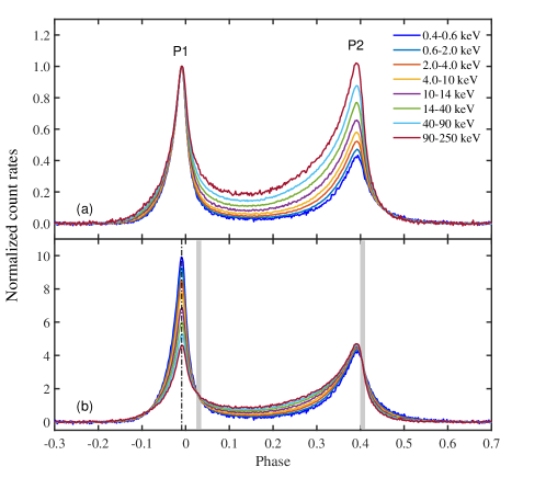
Figure 1: The normalized profiles of the Crab pulsar in different energy bands from NICER and Insight-HXMT’s observations. The whole phase range is divided into 500 bins. The profiles in 0.4–10 keV are from NICER’s observations, and in 10–250 keV from Insight-HXMT’s observations. In panel (a), profiles are normalized by the peak intensity of P1 with the off-pulse emission subtracted; In panel (b), profiles are normalized by the mean count rates of all phase bins with the off-pulse emission subtracted. The dash-dotted line marks the location of the P1, and two gray bars (phase 0.025–0.035, and 0.40–0.41) mark the turnover phase positions of the spectral index variation trends.

3.2 Parameterization of the Pulse Profiles

In order to study the energy dependence of the pulses more comprehensively, we describe the shape of a pulse profile with five parameters, which are the ratio of the peak intensity of P2 to that of P1 ($R_{I}$), the separation of the two pulses ($\Delta{\Phi}$), the full width at half maximum (FWHM) of P1 ($W_{1}$), the FWHM of P2 ($W_{2}$), and the ratio of the fluxes within the FWHM phase ranges ($R_{F}$) of the two pulses. Because the shapes including the peak phases of the two pulses change with energy, the evolution of $R_{F}$ with energy differs slightly from that of $R_{I}$. The peak intensities and phase positions of the two pulses are obtained by using the empirical formula proposed by Nelson et al. (1970), as introduced in Ge et al. (2012).

To explore the exact profile evolution of the pulses from another aspect, we calculate the flux ratios between the left side and the right side of P1 and P2 in different energy bins. The four phase intervals from which the fluxes are calculated are: LP1 (from the left FWHM phase to the peak of P1), RP1 (from the peak of P1 to its right FWHM phase to the peak of P1), LP2 (from the left FWHM phase to the peak of P2), RP2 (from the peak of P2 to its right FWHM phase to the peak of P2).

3.3 Spectral Fitting

The XSPEC (v.12.10.0c) in the software package HEASOFT is used to fit the spectra created in Section 2. The PRS of the Crab pulsar extracted from the NICER observations were fitted by a power law model by Vivekanand (2021), and the similar spectral analyses of the Insight-HXMT data were also carried out by Tuo et al. (2019). In this work, we fit the PRS from NICER and Insight-HXMT data jointly, with the log-parabola model (Massaro et al., 2000) and the broken power law models, respectively.

The log-parabola model involves three components, wabs*constant*logpar, among which wabs accounts for the interstellar medium absorption whose column density $N_{H}$ is fixed as 0.36$\times 10^{22}$ cm^-2 (Ge et al., 2012), constant is used to compensate the mis-match of the effective areas of the three instruments (i.e. XTI, ME, and HE), and logpar is a power-law with an index which varies with energy $E$ (eq. 1) to show the detailed energy evolution of the spectrum $F(E)$ (Massaro et al., 2000) in a broad band,

$$F(E)=K(E/E_{0})^{-(\alpha+\beta{log(E/E_{0})})}.$$ (1)

where $E_{0}=$1 keV, and $\alpha$, $\beta$ and the normalization value $K$ are set as free parameters to fit. $\alpha$ corresponds to the photon index at 1 keV, and $\beta$ is used to represent the curvature of the spectrum. The constant for the NICER spectra is fixed at 1, while for the ME and HE spectra, their constant are determined by jointly fitting the phase averaged spectra of the three instruments. As shown in Figure 2, the phase averaged spectra from these three instruments could be well fitted by the logpar model, and the obtained parameters are: constant equal to $0.623\pm 0.002$ and $0.831\pm 0.004$ for ME and HE, respectively, $\alpha=1.581\pm 0.004$, $\beta=0.109\pm 0.001$, $K=0.471\pm 0.002$, and the reduced $\chi^{2}=0.742$ for degree of freedom of 1607. Specifically, the two constant values are used when we fit the PRS.

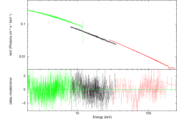
Figure 2: The joint fitting of phase average spectra for NICER and Insight-HXMT’s observations by using the logpar model. The green points are the NICER data in 2–12 keV, the black ones are the HXMT-ME data in 8–35 keV, the red points are the HXMT-HE data in 27–250 keV. The upper and lower panels show the spectra and residuals in terms of sigmas with error bars, respectively.

We also used a two-segment broken power law function (bknpow) and a three-segment broken function (bkn2pow) to search for the turnover energy of a spectrum of the Crab pulsar. Again, a wabs model is used to account for the absorption of the interstellar medium and constant to adjust the mis-match between the instruments. Figure 3 shows the fitting results of a spectrum in phase 0.00–0.01 by using the wabs*constant*bknpow and wabs*constant*bkn2pow models. Compared with the bknpow model, bkn2pow gives a much better fit to the data and so the fitting results of $bkn2pow$ model are discussed later in this work.

One spectrum is created for each phase bin with a size of 0.01 in phase -0.12 to 0.5. These spectra are fitted with the logpar model each. However, some of the spectra are merged into one when fitted with the bkn2pow model in order to improve the statistics. The background spectrum is created using all the events in phase range 0.6-0.8.

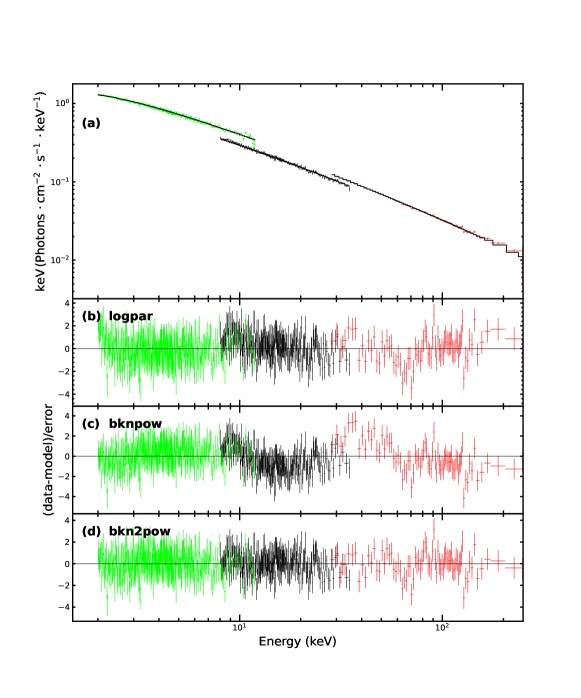
Figure 3: The joint fitting for NICER and Insight-HXMT’s observations in phase 0–0.01. Panel (a) shows the broad band unfolded spectra, the fitting residuals of three models, logpar, bknpow, and bkn2pow, are shown in panel (b), (c) and (d), respectively. The green points are the NICER data in 2–12 keV, the black ones are the HXMT-ME data in 8–35 keV, the red points are the HXMT-HE data in 27–250 keV.

4 Results

4.1 Evolution of the Pulse Profiles with Energy

Our analyses present the evolution of the pulse profiles with energy much more quantitatively than in the previous studies. As shown in Figure 1, the peak intensity ratio and the FWHM of the two pulses all manifest an increasing trend with energy. The intensity of P1 decreases with energy and this trend reverses at phase about 0.035. The intensity of the “bridge” region between this phase and 0.4 increases with energy, and then the intensity starts to decrease with energy again, as displayed in Figure 1(b).

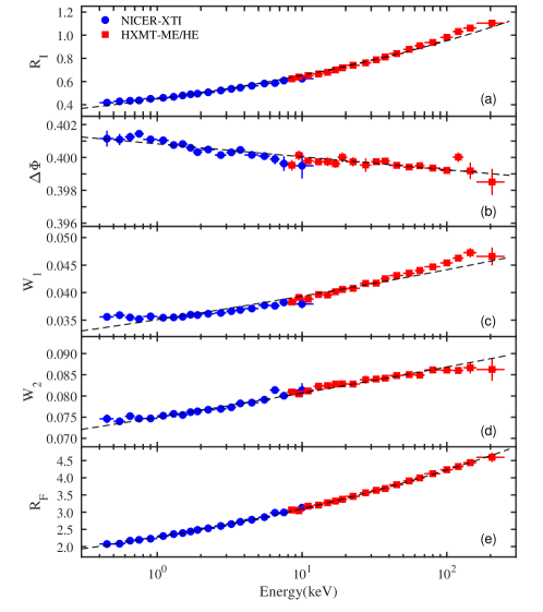
Figure 4: The pulse shape parameters of the Crab pulsar in X-ray. $R_{I}$ is the intensity ratio of two pulses. $\Delta{\Phi}$ is the phase separation of two pulses. $W_{1}$ and $W_{2}$ represent the FWHM of P1 and P2, respectively. $R_{F}$ is used to denote the flux ratio of the two pulses within FWHM. All the shape parameters evolves with energy gradually, and the black dashed lines represent the joint fitting results of data points from the two satellites with a power law function respectively.

Figure 4(a) shows that the intensity ratio of two pulses. $R_{I}$ increases monotonously and becomes higher than 1 above 120 keV. The separation between the two pulses decreases with energy in general, but might increase with energy below 0.8 keV (Figure 4(b)). The pulse widths shown in panels (c) and (d) increase with energy, albeit with different slopes. The flux ratio of two pulses ($R_{F}$) also increases with energy, from $2.08\pm 0.03$ at 0.45 keV to $4.60\pm 0.14$ at about 200 keV, with a slightly larger gradient than that of $R_{I}$ (panel(e)).

In order to quantify the evolutionary trends of the above parameters, we try to fit the data points with different models and find that the power law function $Y=c_{1}*E(keV)^{c_{2}}$ can give an acceptable fit, where $Y$ represents different shape parameters, and $c_{1}$ and $c_{2}$ are coefficients of the evolution. All the data points from NICER and Insight-HXMT are fitted, and the parameters are listed in Table 1.

Table 1: The fitted results of the pulse shapes with a power law model.

$Y$	$c_{1}$	$c_{2}$
	$\times{10^{-2}}$	$\times{10^{-2}}$
$R_{I}$	$44.84\pm 0.18$	$16.36\pm 0.18$
$\Delta{\Phi}$	$40.083\pm 0.005$	$-0.086\pm 0.005$
$W_{1}$	$3.51\pm 0.01$	$5.00\pm 0.19$
$W_{2}$	$7.49\pm 0.01$	$3.20\pm 0.06$
$R_{F}$	$227.35\pm 0.23$	$13.47\pm 0.05$
$R_{F,P2/P1}$	$93.47\pm 0.11$	$13.78\pm 0.05$
$R_{F,Bridge/P1}$	$23.60\pm 0.09$	$27.92\pm 0.12$

Flux ratios of the left side to the right side are also obtained for the two pulses respectively to represent the evolution of their shapes with energy, which are given in Figure 5. Combining with the results in Figure 4, we find that as the photon energy increases, (1) the flux of P1 relative to the entire flux drops, leading to a broader pulse and a lower height peak; the flux ratio between the left side and the right side of P1 decreases slightly; (2) the flux ratio of P2 relative to the entire flux rises, leading to a broader pulse and a higher peak height; the flux ratio between the left side and the right side of P2 increases obviously; (3) the flux of the bridge region relative to the entire flux rises; (4) the change trend of pulse intensity turns over at the phases about 0.035 and 0.4, which are not aligned with the peak positions of P1 and P2.

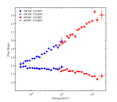
Figure 5: The flux ratio between the left side and the right side of P1 and P2. The phase definitions are declared in Section 3.2.

In order to compare our observational results with the theoretic prediction of the outer gap model in Zhang & Cheng (2002), flux ratios ($R_{F,P2/P1}$, $R_{F,Bridge/P1}$) are calculated according to the phase intervals used in their work, which are (-0.05, 0.05) for P1, (0.05, 0.27) for Bridge, and (0.27, 0.47) for P2. Apparently, as shown in Figure 6, Zhang & Cheng (2002)’s model can produce qualitatively the observed trend, but their exact functional relationship between flux ratio and energy is not accord with the results in this work.

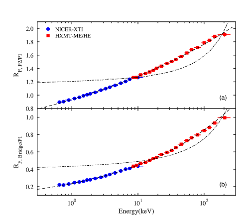
Figure 6: The flux ratios of the Crab pulsar using the phase intervals defined in Zhang & Cheng (2002), which are (-0.05,0.05) for P1, (0.05,0.27) for Bridge, and (0.27,0.47) for P2. The dash-dotted lines in panel (a) and (b) are the expected evolution trends of flux ratios for the model in Zhang & Cheng (2002). The dashed lines represent the evolution trends of flux ratios from observations.

4.2 Phase-resolved Spectra

The fitted parameters of the PRS by the log-parabola model are displayed in Figure 7, and their values and fitting goodness are listed in Table 2. As can be seen in Figure 7(a), the phase resolved spectral properties of the two pulses are quite different: the spectral index $\alpha$ around P1 increases first and then falls off, with the maximum at the peak; and $\alpha$ keeps growing from the leading wing to the trailing wing of P2. In the bridge region, $\alpha$ has a down and up trend, and changes smoothly with phase. The values of the curvature parameter $\beta$ for all the spectra are positive ( Figure 7(b) ), meaning that the spectral index increases with energy at all phases. $\beta$ presents a “W” shape in phase and reaches the local minimum around two turning points of the pulse profiles. Both $\alpha$ and $\beta$ in 2-250 keV show phase evolution trends similar to those in Ge et al. (2012), but with higher precision. The value of $\beta$ in 2-250 keV is smaller than in 3-60 keV, indicating that the photon index changes more slowly at higher energies. The phase turning points of $\beta$ in this work (gray phase regions in Figure 7(b)) are not aligned with those in Ge et al. (2012), probably due to the spectral complexity of this pulsar, because the energy ranges of the two studies are different.

As shown in Figure 3, in phase interval 0-0.01, the fitting reduced $\chi^{2}$ are 1.05, 1.23, 1.03 when using $logpar$, $bknpow$, and $bkn2pow$ models, respectively. The two-segment broken power law model does not result in statistically acceptable fit to the broad band PRS, whereas a three-segment broken power law model can fit the spectra very well. The joint fitting parameters for PRS by using a three-segment broken power law are shown in Figure 8 and listed in Table 3. It can be seen that the three spectral indices ($\Gamma_{1}$, $\Gamma_{2}$, $\Gamma_{3}$) all change with phase and their evolution trends are similar, and distributions of the differences between them are consistent with the evolution of $\beta$ with phase. $E_{break,1}$ changes rather randomly, but $E_{break,2}$ is positively correlated with $\beta$. Madsen et al. (2015) found that the 3-78 keV PRS extracted from the NuSTAR observations can be well fitted with a two-segment power-law function (bknpow), with the break energy fixed at 11.7 keV or 13.1 keV. Comparing with our results, we found that these two break energies are comparable with $E_{break,1}$ and the evolutions of the photon indices share the similar trend. According to the fitting results in Table 3, the reduced $\chi^{2}$ is higher and closer to 1 in the phase intervals near P1 and P2 than that in the bridge intervals, it means the bkn2pow model is more suitable for the spectra fitting of P1 and P2, but the spectra in the other phase intervals with lower statistics could be over fitted with such a model. It should be noted that the NuSTAR results (Madsen et al., 2015) also support our results that the turnover or bending at high energies are around a few tens of keV.

Some fitting parameters of logpar and bkn2pow models have clear correlations in certain phase intervals. As shown in Figure 9(a), the correlation between $\alpha$ and $\beta$ are opposite on both sides of P1 before reaching the first phase turning point. Between the two phase turning points, there is a significant anti-correlation between $\alpha$ and $\beta$, but their functional relationship seem to be not the same for two groups of data, in phase 0.04-0.25 and 0.25-0.41 respectively (Figure 9(b)). At the right side of P2, the correlation between $\alpha$ and $\beta$ is unclear, perhaps due to the limitation of statistics (Figure 9(c)). For the bkn2pow model, we only find a possible anti-correlation between the averaged indices (($\Gamma_{1}+\Gamma_{2}+\Gamma_{3}$)/3) and $E_{break,2}$ in phase 0.03-0.40, and their exact functional relationship also seems to be not the same in the front and rear phase intervals of the bridge region, as shown in Figure 10.

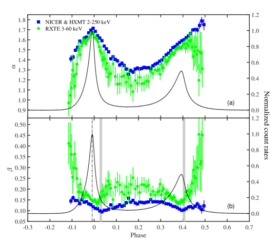
Figure 7: Fitting results of the PRS of the Crab pulsar using a log-parabola model, where these blue squared data points are the joint fitting results from NICER and Insight-HXMT’s observations which cover 2-250 keV, and the green circled data points are the fitting results for RXTE’s observations presented in Ge et al. (2012). The dash-dotted line marks the peak location of the primary pulse P1, and the two gray bars mark the shape turnover phase intervals, as shown in Figure 1.

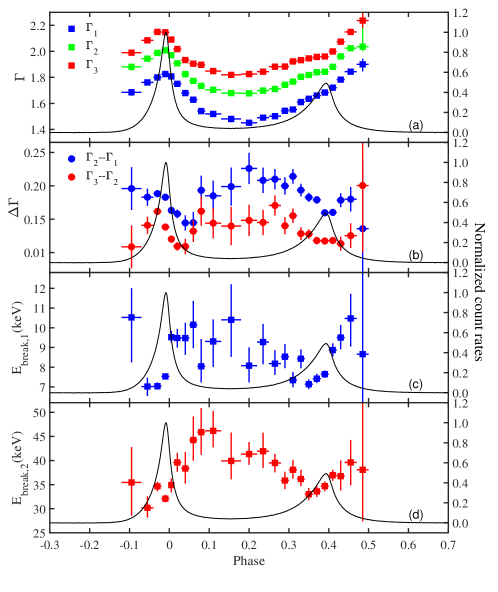
Figure 8: Joint fitting results of the PRS of the Crab pulsar using a three-segment broken power law model (bkn2pow) for X-ray observations in 2–250 keV. Panel (a),(c),(d): the parameters in the bkn2pow model, and panel (b) displays the differences among three indices in panel (a).

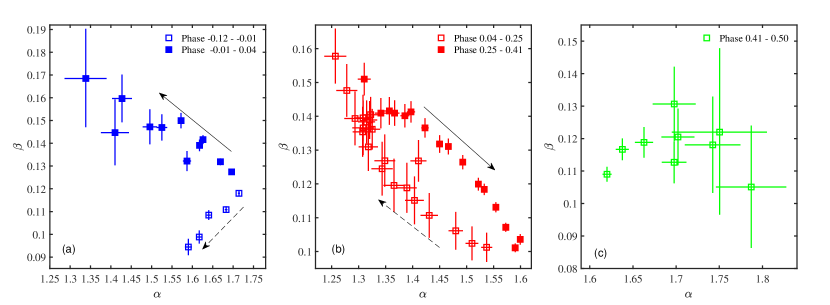
Figure 9: The correlations between $\alpha$ and $\beta$ in different phase intervals. The black dashed and solid arrows indicate the direction of phase increasing for their surrounding hollow and solid data points, respectively.

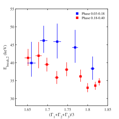
Figure 10: The correlations between the average photon indices and $E_{break,2}$ of the spectral model $bkn2pow$ in different phase intervals.

Table 2: The Phase-resolved Spectral Analysis Results of the Crab Pulsar for a Log-parabola Model (logpar) in 2-250 keV

Phase Range	$\alpha$	$\beta$	Normalization	Reduced $\chi^{2}$
0 - 0.01	$1.683\pm 0.003$	$0.111\pm 0.001$	$2.512\pm 0.008$	1.05
0.01 - 0.02	$1.640\pm 0.005$	$0.108\pm 0.002$	$1.414\pm 0.007$	1.04
0.02 - 0.03	$1.617\pm 0.007$	$0.099\pm 0.003$	$0.913\pm 0.007$	1.01
0.03 - 0.04	$1.590\pm 0.008$	$0.094\pm 0.004$	$0.643\pm 0.006$	0.99
0.04 - 0.05	$1.537\pm 0.010$	$0.101\pm 0.004$	$0.470\pm 0.005$	1.02
0.05 - 0.06	$1.510\pm 0.012$	$0.102\pm 0.005$	$0.372\pm 0.005$	1.03
0.06 - 0.07	$1.480\pm 0.013$	$0.106\pm 0.006$	$0.308\pm 0.005$	1.01
0.07 - 0.08	$1.411\pm 0.015$	$0.127\pm 0.006$	$0.250\pm 0.005$	1.01
0.08 - 0.09	$1.431\pm 0.016$	$0.111\pm 0.007$	$0.225\pm 0.004$	1.04
0.09 - 0.10	$1.403\pm 0.017$	$0.115\pm 0.007$	$0.199\pm 0.004$	1.06
0.10 - 0.11	$1.389\pm 0.018$	$0.119\pm 0.007$	$0.184\pm 0.004$	0.97
0.11 - 0.12	$1.348\pm 0.019$	$0.127\pm 0.008$	$0.162\pm 0.004$	1.05
0.12 - 0.13	$1.366\pm 0.020$	$0.120\pm 0.008$	$0.161\pm 0.004$	0.99
0.13 - 0.14	$1.343\pm 0.020$	$0.124\pm 0.008$	$0.154\pm 0.004$	1.04
0.14 - 0.15	$1.308\pm 0.020$	$0.137\pm 0.008$	$0.145\pm 0.004$	1.00
0.15 - 0.16	$1.257\pm 0.020$	$0.158\pm 0.008$	$0.137\pm 0.004$	1.01
0.16 - 0.17	$1.293\pm 0.020$	$0.139\pm 0.008$	$0.142\pm 0.004$	1.00
0.17 - 0.18	$1.278\pm 0.019$	$0.148\pm 0.008$	$0.145\pm 0.004$	1.01
0.18 - 0.19	$1.307\pm 0.018$	$0.135\pm 0.007$	$0.156\pm 0.004$	0.98
0.19 - 0.20	$1.318\pm 0.018$	$0.131\pm 0.007$	$0.164\pm 0.004$	1.00
0.20 - 0.21	$1.308\pm 0.017$	$0.140\pm 0.007$	$0.175\pm 0.004$	0.97
0.21 - 0.22	$1.315\pm 0.016$	$0.138\pm 0.006$	$0.191\pm 0.004$	1.02
0.22 - 0.23	$1.325\pm 0.015$	$0.136\pm 0.006$	$0.206\pm 0.004$	1.00
0.23 - 0.24	$1.320\pm 0.014$	$0.139\pm 0.006$	$0.222\pm 0.004$	0.98
0.24 - 0.25	$1.322\pm 0.013$	$0.140\pm 0.005$	$0.242\pm 0.004$	1.02
0.25 - 0.26	$1.310\pm 0.012$	$0.151\pm 0.005$	$0.266\pm 0.004$	1.00
0.26 - 0.27	$1.341\pm 0.011$	$0.141\pm 0.004$	$0.303\pm 0.004$	1.04
0.27 - 0.28	$1.357\pm 0.010$	$0.142\pm 0.004$	$0.348\pm 0.004$	1.05
0.28 - 0.29	$1.367\pm 0.009$	$0.141\pm 0.004$	$0.393\pm 0.004$	1.06
0.29 - 0.30	$1.386\pm 0.008$	$0.140\pm 0.003$	$0.456\pm 0.005$	1.00
0.30 - 0.31	$1.397\pm 0.008$	$0.141\pm 0.003$	$0.523\pm 0.005$	1.00
0.31 - 0.32	$1.423\pm 0.007$	$0.137\pm 0.003$	$0.615\pm 0.005$	0.95
0.32 - 0.33	$1.450\pm 0.006$	$0.132\pm 0.003$	$0.726\pm 0.005$	0.98
0.33 - 0.34	$1.466\pm 0.006$	$0.131\pm 0.002$	$0.851\pm 0.005$	1.05
0.34 - 0.35	$1.493\pm 0.005$	$0.126\pm 0.002$	$1.017\pm 0.006$	1.02
0.35 - 0.36	$1.522\pm 0.004$	$0.120\pm 0.002$	$1.218\pm 0.006$	1.02
0.36 - 0.37	$1.533\pm 0.004$	$0.118\pm 0.002$	$1.426\pm 0.006$	1.05
0.37 - 0.38	$1.554\pm 0.003$	$0.113\pm 0.001$	$1.699\pm 0.006$	1.12
0.38 - 0.39	$1.573\pm 0.003$	$0.107\pm 0.001$	$1.966\pm 0.007$	1.01
0.39 - 0.40	$1.590\pm 0.003$	$0.101\pm 0.001$	$2.072\pm 0.007$	1.07
0.40 - 0.41	$1.599\pm 0.004$	$0.104\pm 0.002$	$1.739\pm 0.007$	1.07
0.41 - 0.42	$1.620\pm 0.005$	$0.109\pm 0.002$	$1.248\pm 0.007$	1.01
0.42 - 0.43	$1.638\pm 0.008$	$0.117\pm 0.003$	$0.901\pm 0.007$	0.97
0.43 - 0.44	$1.663\pm 0.010$	$0.119\pm 0.005$	$0.683\pm 0.007$	1.02
0.44 - 0.45	$1.698\pm 0.014$	$0.113\pm 0.006$	$0.530\pm 0.008$	0.94
0.45 - 0.46	$1.702\pm 0.019$	$0.120\pm 0.009$	$0.407\pm 0.008$	0.96
0.46 - 0.47	$1.698\pm 0.025$	$0.131\pm 0.011$	$0.320\pm 0.008$	1.09
0.47 - 0.48	$1.742\pm 0.032$	$0.118\pm 0.015$	$0.260\pm 0.008$	1.08
0.48 - 0.49	$1.787\pm 0.041$	$0.105\pm 0.019$	$0.217\pm 0.009$	1.02
0.49 - 0.50	$1.750\pm 0.055$	$0.122\pm 0.026$	$0.159\pm 0.009$	1.00
0.88 - 0.89	$1.338\pm 0.052$	$0.168\pm 0.022$	$0.070\pm 0.004$	1.03
0.89 - 0.90	$1.410\pm 0.034$	$0.145\pm 0.014$	$0.114\pm 0.005$	1.05
0.90 - 0.91	$1.427\pm 0.024$	$0.160\pm 0.010$	$0.182\pm 0.005$	1.05
0.91 - 0.92	$1.496\pm 0.018$	$0.147\pm 0.008$	$0.287\pm 0.006$	1.01
0.92 - 0.93	$1.525\pm 0.013$	$0.147\pm 0.006$	$0.423\pm 0.006$	1.03
0.93 - 0.94	$1.587\pm 0.010$	$0.132\pm 0.004$	$0.628\pm 0.007$	1.11
0.94 - 0.95	$1.572\pm 0.008$	$0.150\pm 0.003$	$0.870\pm 0.007$	1.05
0.95 - 0.96	$1.618\pm 0.006$	$0.139\pm 0.003$	$1.271\pm 0.007$	1.01
0.96 - 0.97	$1.626\pm 0.004$	$0.142\pm 0.002$	$1.784\pm 0.008$	1.13
0.97 - 0.98	$1.669\pm 0.003$	$0.132\pm 0.001$	$2.658\pm 0.009$	1.08
0.98 - 0.99	$1.696\pm 0.002$	$0.127\pm 0.001$	$3.898\pm 0.010$	1.12
0.99 - 1.00	$1.714\pm 0.002$	$0.118\pm 0.001$	$4.226\pm 0.010$	1.20

Table 3: The Phase-resolved Spectral Analysis Results of the Crab Pulsar for a Three-segment Broken Function Model (bkn2pow) in 2-250 keV

Phase Range	$\Gamma_{1}$	$\Gamma_{2}$	$\Gamma_{3}$	$E_{break,1}$	$E_{break,2}$	Normalization	Reduced $\chi^{2}$
0 - 0.01	$1.807_{-0.003}^{+0.003}$	$1.970_{-0.004}^{+0.004}$	$2.090_{-0.005}^{+0.005}$	$9.523_{-0.269}^{+0.308}$	$34.907_{-1.516}^{+1.353}$	$2.663_{-0.009}^{+0.009}$	1.03
0.01 - 0.03	$1.750_{-0.005}^{+0.004}$	$1.908_{-0.005}^{+0.004}$	$2.017_{-0.006}^{+0.005}$	$9.482_{-0.486}^{+0.459}$	$39.610_{-1.922}^{+1.970}$	$1.236_{-0.007}^{+0.007}$	0.75
0.03 - 0.05	$1.680_{-0.008}^{+0.008}$	$1.824_{-0.008}^{+0.008}$	$1.933_{-0.008}^{+0.010}$	$9.478_{-0.850}^{+0.773}$	$38.351_{-3.120}^{+3.376}$	$0.592_{-0.006}^{+0.007}$	0.73
0.05 - 0.07	$1.628_{-0.013}^{+0.012}$	$1.773_{-0.011}^{+0.010}$	$1.905_{-0.014}^{+0.015}$	$10.154_{-1.188}^{+1.206}$	$44.248_{-4.268}^{+4.892}$	$0.369_{-0.006}^{+0.006}$	0.76
0.07 - 0.09	$1.541_{-0.017}^{+0.021}$	$1.734_{-0.010}^{+0.010}$	$1.896_{-0.017}^{+0.019}$	$8.046_{-0.825}^{+1.382}$	$45.878_{-4.701}^{+5.009}$	$0.253_{-0.005}^{+0.007}$	0.69
0.09 - 0.13	$1.519_{-0.023}^{+0.019}$	$1.704_{-0.008}^{+0.009}$	$1.848_{-0.014}^{+0.017}$	$9.308_{-1.296}^{+1.117}$	$46.170_{-3.425}^{+4.116}$	$0.192_{-0.005}^{+0.005}$	0.60
0.13 - 0.18	$1.481_{-0.026}^{+0.022}$	$1.679_{-0.013}^{+0.018}$	$1.819_{-0.010}^{+0.014}$	$10.404_{-1.874}^{+1.798}$	$39.911_{-3.808}^{+5.892}$	$0.163_{-0.006}^{+0.005}$	0.58
0.18 - 0.22	$1.451_{-0.024}^{+0.020}$	$1.677_{-0.008}^{+0.007}$	$1.825_{-0.010}^{+0.010}$	$8.079_{-0.851}^{+0.926}$	$41.344_{-2.218}^{+2.491}$	$0.185_{-0.006}^{+0.005}$	0.55
0.22 - 0.25	$1.491_{-0.017}^{+0.016}$	$1.699_{-0.010}^{+0.009}$	$1.844_{-0.011}^{+0.014}$	$9.274_{-1.123}^{+0.920}$	$41.941_{-3.489}^{+3.832}$	$0.249_{-0.005}^{+0.006}$	0.59
0.25 - 0.28	$1.501_{-0.015}^{+0.013}$	$1.711_{-0.007}^{+0.007}$	$1.882_{-0.008}^{+0.008}$	$8.182_{-0.569}^{+0.681}$	$39.501_{-1.953}^{+1.876}$	$0.337_{-0.006}^{+0.006}$	0.64
0.28 - 0.30	$1.543_{-0.011}^{+0.011}$	$1.743_{-0.006}^{+0.007}$	$1.883_{-0.007}^{+0.007}$	$8.533_{-0.584}^{+0.641}$	$35.861_{-1.785}^{+1.806}$	$0.471_{-0.007}^{+0.006}$	0.75
0.30 - 0.32	$1.553_{-0.008}^{+0.011}$	$1.767_{-0.005}^{+0.006}$	$1.922_{-0.006}^{+0.007}$	$7.342_{-0.356}^{+0.410}$	$38.067_{-1.835}^{+2.039}$	$0.615_{-0.006}^{+0.008}$	0.70
0.32 - 0.34	$1.610_{-0.008}^{+0.008}$	$1.804_{-0.005}^{+0.005}$	$1.932_{-0.005}^{+0.005}$	$8.429_{-0.481}^{+0.469}$	$36.172_{-1.485}^{+1.893}$	$0.865_{-0.008}^{+0.008}$	0.77
0.34 - 0.36	$1.635_{-0.006}^{+0.005}$	$1.818_{-0.004}^{+0.004}$	$1.946_{-0.004}^{+0.004}$	$7.138_{-0.249}^{+0.251}$	$33.010_{-1.236}^{+1.281}$	$1.200_{-0.009}^{+0.008}$	0.74
0.36 - 0.38	$1.660_{-0.004}^{+0.005}$	$1.839_{-0.004}^{+0.003}$	$1.957_{-0.003}^{+0.003}$	$7.416_{-0.221}^{+0.255}$	$33.604_{-1.158}^{+1.079}$	$1.664_{-0.008}^{+0.009}$	0.79
0.38 - 0.40	$1.683_{-0.003}^{+0.003}$	$1.843_{-0.003}^{+0.003}$	$1.960_{-0.003}^{+0.003}$	$7.648_{-0.193}^{+0.184}$	$34.687_{-1.034}^{+0.966}$	$2.134_{-0.008}^{+0.008}$	0.74
0.40 - 0.42	$1.721_{-0.005}^{+0.004}$	$1.881_{-0.003}^{+0.003}$	$1.999_{-0.004}^{+0.004}$	$8.867_{-0.320}^{+0.343}$	$36.959_{-1.174}^{+1.129}$	$1.585_{-0.009}^{+0.008}$	0.72
0.42 - 0.44	$1.783_{-0.007}^{+0.007}$	$1.961_{-0.007}^{+0.008}$	$2.074_{-0.009}^{+0.010}$	$9.506_{-0.595}^{+0.636}$	$36.757_{-2.960}^{+3.254}$	$0.853_{-0.008}^{+0.007}$	0.69
0.44 - 0.47	$1.844_{-0.014}^{+0.012}$	$2.024_{-0.013}^{+0.014}$	$2.149_{-0.020}^{+0.020}$	$10.473_{-1.419}^{+1.250}$	$39.611_{-4.762}^{+4.655}$	$0.456_{-0.007}^{+0.007}$	0.62
0.47 - 0.50	$1.900_{-0.055}^{+0.043}$	$2.036_{-0.037}^{+0.138}$	$2.237_{-0.059}^{+0.639}$	$8.662_{-2.993}^{+15.236}$	$38.089_{-10.670}^{+108.327}$	$0.231_{-0.013}^{+0.013}$	0.66
0.88 - 0.93	$1.685_{-0.026}^{+0.016}$	$1.881_{-0.030}^{+0.019}$	$1.990_{-0.014}^{+0.016}$	$10.522_{-2.271}^{+1.485}$	$35.456_{-6.917}^{+7.339}$	$0.249_{-0.007}^{+0.006}$	0.59
0.93 - 0.96	$1.761_{-0.010}^{+0.010}$	$1.944_{-0.009}^{+0.008}$	$2.085_{-0.006}^{+0.006}$	$7.022_{-0.478}^{+0.444}$	$30.206_{-2.023}^{+2.375}$	$1.023_{-0.011}^{+0.011}$	0.66
0.96 - 0.98	$1.799_{-0.004}^{+0.003}$	$1.988_{-0.003}^{+0.003}$	$2.149_{-0.004}^{+0.004}$	$7.036_{-0.172}^{+0.192}$	$34.647_{-1.024}^{+0.926}$	$2.424_{-0.010}^{+0.010}$	0.81
0.98 - 1.00	$1.825_{-0.002}^{+0.003}$	$2.008_{-0.003}^{+0.002}$	$2.146_{-0.003}^{+0.003}$	$7.532_{-0.130}^{+0.135}$	$32.085_{-0.738}^{+0.774}$	$4.354_{-0.012}^{+0.013}$	0.82

5 Discussion

5.1 Comparisons with the Previous Works

The evolution of the flux ratio of the two pulses, one of the most frequently used parameters to describe the pulse profile evolution in X-rays, is consistent with the previous work in Kuiper et al. (2001) and Tuo et al. (2019), but the current results are much more precise and cover a wider energy range of 0.4-250 keV. A multicomponent model in Massaro et al. (2006) is able to reproduce the pulse profiles in different energy bands and the evolution of the flux ratio between P2 and P1 (Kuiper et al., 2001). The flux ratio of two pulses in 0.4-250 keV in this work coincides with that in Kuiper et al. (2001) when using the same phase definitions for P1 and P2, so our results can be also explained by the multicomponent model in Massaro et al. (2006).

Zhang & Cheng (2002) once fit the flux ratios of P2 to P1 and Bridge to P1 by using an outer gap model. However, as shown in Figure 6, there are obvious discrepancies between the predictions of their model and our results. The three-dimensional model in Zhang & Cheng (2002) is based on a rotating vacuum dipole, in which some processes are simplified or unreliable. For example, only photons emitting tangent to the local magnetic field lines are considered, but particles with large initial pitch angles may also emit in other directions. The magnetic inclination and viewing angles used in their work are from old theoretical works, which have not been well determined by observations and are therefore probably inaccurate. More over, the hard X-ray spectral indices they adopted are from old observations and with large uncertainties. These factors may lead to the discrepancies between model predictions and observational results. Therefore, more details need to be added and/or refined into the outer gap model of Zhang & Cheng (2002) to explain the new results in this work.

There are several studies on the spectrum of the Crab pulsar as a function of phase (Pravdo et al., 1997; Massaro et al., 2000, 2006; Mineo et al., 2006; Ge et al., 2012; Tuo et al., 2019; Li et al., 2019; Yeung, 2020). When fitting the spectrum by using a power law model, the overall behaviors of photon indices are very similar, and indices increase clearly with energy over all the phase intervals, i.e., the higher the energy, the softer the spectra are. For the energy curvature trend of spectra which is described by $\beta$ of the log-parabola model fitting, this work gives a more detailed phase evolution trend and obtains links between the spectrum curvature and the evolution of pulse profiles with energy, as shown in Figure 1(b) and Figure 7. The uncertainties of $\alpha$ and $\beta$ are about one fifth of those in Ge et al. (2012).

5.2 Constraints on Pulsar Radiation Models

We can use the energy dependence of the pulse profiles and the PRS to test the pulsar high energy emission models. One of the most popular models in the past is the two-gap outer gap model, proposed by Cheng, Ho, and Ruderman (Cheng et al., 1986a, b). In this model, the gap is “stratified” in energy, and lower energy radiation emanates from a region farther from the neutron star surface than higher energy radiation. The delay between the radio and X-ray pulses decreases significantly with increasing X-ray energy, which indicates that the softer X-ray photons originate from higher altitudes (Molkov et al., 2010). Qualitatively, the energy evolution trends of the pulse shape and spectral index of the Crab pulsar obtained in this paper all conform to the “stratified” structure of this outer gap model. The gap closer to the neutron star surface may cover a larger angular size (relative to the neutron star center) as indicated by the increasing widths of the two pulses with energy. Because the magnetic field in deeper magnetosphere is stronger and P2 becomes more prominent at higher energy, the particle generation (and thus synchrotron emission) in the region close to the neutron star surface and corresponds to P2 maybe more intense (Cheng et al., 2000). According to the energy evolution trend of the whole pulse profiles, the pulse intensity of P1 changes more distinctly than P2, and corresponding radiation area of P1 may be longer and narrower than P2.

In recent years, global PIC simulations were used to model the pulsar magnetosphere (such as Philippov & Spitkovsky (2014); Cerutti et al. (2016); Philippov & Spitkovsky (2018)). In these simulations, the high energy emissions are mainly produced in current sheets just beyond the light cylinder. Cerutti et al. (2016) modeled the pulse profiles and phase-averaged spectra produced by synchrotron radiation process at different viewing and magnetic inclination angles. When the viewing angle is $\sim$ 90-100^∘ and the magnetic inclination is $\sim$ 30-45^∘, the model predicted spectra and pulse profiles of the Crab pulsar are well consistent with the observational results in energy band from soft X-ray to $\gamma$-ray as presented in Kuiper et al. (2001). The PIC simulations and modeling show that electrons and positrons are generated mainly within the magnetosphere. Near the pulsar surface, the electric potential is highest in the equatorial plane and decreases toward the poles for a quasi-aligned rotator (Goldreich & Julian, 1969). The freshly generated positrons in the magnetosphere are accelerated outward to high energy in the reconnection regions outside the light cylinder, where electrons coming from farther in the equatorial plane are accelerated inward. Because the supply of outgoing positrons is much higher than the ingoing electrons, high energy radiation is mainly generated by positrons for a quasi-aligned rotator (Cerutti et al., 2016), and on the contrary, for an anti-aligned rotator, it is expected that the high energy radiation is generated mainly by electrons. The highest energy that a positron can acquire is determined by the accelerating electric field in the reconnection region, multiplied by the acceleration distance that is available in the undulating current sheet. As a consequence, the spectrum will be harder for a lower magnetic inclination angle. On the other hand, charged particles in the current sheet can screen the accelerating electric field (Philippov & Spitkovsky, 2018). These combined factors imply that the high intensity of P1 in low energy band is generated by regions where positrons are more numerous and therefore electric yielding is more significant. In higher energy band, the intensity of P2 becomes higher because P2 is likely produced by regions where electric yielding is weak and positrons can be accelerated to higher energy. The spectra of the bridge component are harder than those of both P1 and P2, while its intensity is lower than P1 and P2. This behavior can also be explained if the bridge component is generated by regions where positron density is lower and the fraction of high energy positron is higher. Future comparison between simulations of the current sheet in different energy bands with the results in our paper could provide more detailed information about the particle acceleration and radiation in the reconnection regions.

Weisskopf et al. (2011) reported that the soft X-ray spectral index has an abrupt change in phase 0.83-0.95, where transition structures of the optical and X-ray polarization properties were also detected (Słowikowska et al., 2009; Vadawale et al., 2018). We find that around that phase the break energies of the bkn2pow are the lowest. It is yet unknown whether these properties are physically associated. Besides this, just behind the two pulses the polarization degree has two local minimum points, where the values of $\beta$ are also the lowest. We speculate that in the two corresponding regions the particles evolve the least due to the lowest magnetic field, which could be less regulated and thus the radiations are less polarized.

6 Summary

In this work, we adopt the observations from NICER and Insight-HXMT, and study the pulse profile and spectrum of the Crab pulsar systematically. The main results and conclusions are: (1) in 0.4-250 keV, the intensity/flux ratio of two pulses show an increasing trend with energy, so do the widths of the two pulses; the separation of the two pulses decreases with energy; the energy evolution trends of the two sides of P1 and P2 are asymmetric; (2) in 2-250 keV, where the spectral shape is not significantly affected by the chemical composition of the absorption interstellar medium, the spectral index increases with energy over all the phase intervals; the spectral index changes more slowly at higher energies; the change of spectral index reaches its local minimum around phase 0.035 and 0.4 that are later than the peak phase of P1 and P2; there are obvious energy breaks on the spectra near the two peaks of the Crab pulsar, and the break energies are generally higher in the region bridging the two pulses; (3) the energy evolution trends of pulse profile and spectrum conform to results in previous studies qualitatively, but more accurate to allow for a detailed analysis; (4) the anti-correlations among spectral fitting parameters ($\alpha$ and $\beta$) indicate that the highest energy particles are produced in regions where the radiation energy loss is also the strongest. We simply compared our results with the predictions of the outer gap model and the PIC simulations of pulsar magnetosphere. It turns out that the theoretical models need to be further refined to explain the details of the observational results.

References

- Abdo et al. (2010) Abdo, A. A., Ackermann, M., Ajello, M., et al. 2010, ApJ, 708, 1254
- Arzamasskiy & Tchekhovskoy (2015) Arzamasskiy, L., Philippov, A., & Tchekhovskoy, A. 2015, MNRAS, 453, 3540
- Campana et al. (2009) Campana, R., Massaro, E., Mineo, T., Cusumano, G. 2009, A&A, 499, 847
- Cerutti et al. (2016) Cerutti, B., Philippov, A. A., & Spitkovsky, A. 2016, MNRAS, 457, 2401.
- Cheng et al. (1986a) Cheng, K. S.; Ho, C.; Ruderman, M. 1986a, ApJ, 300, 500
- Cheng et al. (1986b) Cheng, K. S.; Ho, C.; Ruderman, M. 1986b, ApJ, 300, 522
- Cheng et al. (2000) Cheng, K. S., Ruderman, M., & Zhang, L. 2000, ApJ, 537, 964
- Eikenberry & Fazio (1997) Eikenberry, S. S. & Fazio, G. G. 1997, ApJ, 476, 281
- Enoto et al. (2021) Enoto, T., Terasawa, T., Kisaka, S., et al. 2021, Science, 372, 187. doi:10.1126/science.abd4659
- Ge et al. (2012) Ge, M. Y., Lu, F. J., Qu, J. L., et al. 2012, ApJS, 199, 32
- Ge et al. (2016) Ge, M. Y., Yan, L. L., Lu, F. J., et al. 2016, ApJ, 818, 48
- Goldreich & Julian (1969) Goldreich, P. & Julian, W. H. 1969, ApJ, 157, 869.
- Harding et al. (2008) Harding, A. K., Stern, J. V., Dyks, J., Frackowiak, M. 2008, ApJ, 680, 1378
- Kirsch et al. (2005) Kirsch M. G., Abbey A., Altieri B., Baskill D., Dennerl K., van Dooren J., Fauste J., et al., 2005, SPIE, 5898, 224.
- Kuiper et al. (2001) Kuiper, L., Hermsen, W., Cusumano, G., et al. 2001, A&A, 378, 918
- Kuiper et al. (2003) Kuiper, L., Hermsen, W., Walter, R., & Foschini, L. 2003, A&A, 411, L31
- Li et al. (2019) Li, H. C., Gauvin, N., Ge, M. Y., et al. 2019, Journal of High Energy Astrophysics, 24, 15
- Lyne et al. (1993) Lyne, A. G., Pritchard, R. S., & Graham Smith, F. 1993, MNRAS, 265, 1003
- Lyne et al. (2013) Lyne, A., Graham-Smith, F., Weltevrede, P., et al. 2013, Science, 342, 598
- Madsen et al. (2015) Madsen, K. K., Reynolds, S., Harrison, F., et al. 2015, ApJ, 801, 66.
- Massaro et al. (2000) Massaro, E., Cusumano, G., Litterio, M., Mineo, T. 2000, A&A, 361, 695
- Massaro et al. (2006) Massaro, E., Campana, R., Cusumano, G., & Mineo, T. 2006, A&A, 459, 859
- Mineo et al. (2006) Mineo, T., Ferrigno, C., Foschini, L., et al. 2006, A&A, 450, 617
- Molkov et al. (2010) Molkov, S., Jourdain, E., & Roques, J. P. 2010, ApJ, 708, 403
- Nelson et al. (1970) Nelson, J., Hills, R., Cudaback, D., & Wampler, J. 1970, ApJ, 161, L235
- Oosterbroek et al. (2008) Oosterbroek, T., Cognard, I., Golden, A., et al. 2008, A&A, 488, 271
- Philippov & Spitkovsky (2014) Philippov, A. A., & Spitkovsky, A., 2014, ApJ, 785, L33
- Philippov et al. (2015a) Philippov, A. A., Spitkovsky, A., & Cerutti, B. 2015a, ApJ, 801, L19.
- Philippov et al. (2015b) Philippov, A. A., Cerutti, B., Tchekhovskoy, A., et al. 2015b, ApJ, 815, L19.
- Philippov & Spitkovsky (2018) Philippov, A. A. & Spitkovsky, A. 2018, ApJ, 855, 94.
- Pravdo et al. (1997) Pravdo, S. H., Angelini, L., Harding, A. K. 1997, ApJ, 491, 808
- Prigozhin et al. (2016) Prigozhin G., Gendreau K., Doty J. P., Foster R., Remillard R., Malonis A., LaMarr B., et al., 2016, SPIE, 9905, 99051I.
- Rots et al. (2004) Rots, A. H., Jahoda, K., & Lyne, A. G. 2004, ApJ, 605, L129
- Słowikowska et al. (2009) Słowikowska A., Kanbach G., Kramer M., Stefanescu A., 2009, MNRAS, 397, 103
- Takata et al. (2007) Takata, J., Chang, H.-K., & Cheng, K. S. 2007, ApJ, 656, 1044
- Tang et al. (2008) Tang, A. P. S., Takata, J., Jia, J. J., et al. 2008, ApJ, 676, 562
- Tuo et al. (2019) Tuo, Y.-L., Ge, M.-Y., Song, L.-M., et al. 2019, Research in Astronomy and Astrophysics, 19, 087
- Vadawale et al. (2018) Vadawale, S. V., Chattopadhyay, T., Mithun, N. P. S., et al. 2018, Nature Astronomy, 2, 50.
- Vivekanand (2021) Vivekanand M., 2021, A&A, 649, A140
- Weisskopf et al. (2004) Weisskopf, M. C., O’Dell, S. L., Paerels, F., et al. 2004, ApJ, 601, 1050
- Weisskopf et al. (2011) Weisskopf, M. C., Tennant, A. F., Yakovlev, D. G., et al. 2011, ApJ, 743, 139
- Yan et al. (2017) Yan, L. L., Ge, M. Y., Yuan, J. P., et al. 2017, ApJ, 845, 119
- Yan et al. (2018) Yan, L. L., Ge, M. Y., Lu, F. J., et al. 2018, ApJ, 865, 21
- Yeung (2020) Yeung, Paul K. H. 2020, A&A, 640, A43
- Zhang & Cheng (2002) Zhang, L., Cheng, K. S. 2002, ApJ,569, 872
- Zhang & Li (2009) Zhang, L. & Li, X. 2009, ApJ, 707, L169
- Zhang et al. (2020) Zhang S.-N., Li T., Lu F., Song L., Xu Y., Liu C., Chen Y., et al., 2020, SCPMA, 63, 249502