Extracting resonance poles from numerical scattering data: type-II Padé reconstruction

Abstract

We present a FORTRAN 77 code for evaluation of resonance pole positions and residues of a numerical scattering matrix element in the complex energy (CE) as well as in the complex angular momentum (CAM) planes. Analytical continuation of the $S$-matrix element is performed by constructing a type-II Padé approximant from given physical values [Bessis et al (1994); Vrinceanu et al (2000); Sokolovski and Msezane (2004)] . The algorithm involves iterative ’preconditioning’ of the numerical data by extracting its rapidly oscillating potential phase component. The code has the capability of adding non-analytical noise to the numerical data in order to select ’true’ physical poles, investigate their stability and evaluate the accuracy of the reconstruction. It has an option of employing multiple-precision (MPFUN) package [Bailey (1993)] developed by D. H. Bailey wherever double precision calculations fail due to a large number of input partial wave (energies) involved. The package has been successfully tested on several models, as well as the F + H₂ $\rightarrow$ HF + H, F + HD$\rightarrow$ HF + D, Cl + HCl$\rightarrow$ ClH + Cl and H + D₂$\rightarrow$ HD + D reactions. Some detailed examples are given in the text.

PACS:34.50.Lf,34.50.Pi

PROGRAM SUMMARY

Manuscript Title: Extracting resonance poles from numerical scattering data: type-II Padé reconstruction.
Authors: D. Sokolovski, E.Akhmatskaya and S.K.Sen
Program Title: PADE_II
Journal Reference:
Catalogue identifier:
Licensing provisions: Free software license
Programming language: FORTRAN 77
Computer: Any computer equipped with a FORTRAN 90 compiler
Operating system: UNIX, LINUX
RAM: 256 Mb
Has the code been vectorised or parallelised: no
Number of processors used: one
Supplementary material: MPFUN package, validation suite, script files, input files, readme file, Installation and User Guide
Keywords: Resonances, S-matrix; Padé approximation; Regge-poles.
PACS: 34.50.Lf,34.50.Pi
Classification: Molecular Collisions
External routines/libraries: NAG Program Library
CPC Program Library subprograms used: N/A
Nature of problem:
The package extracts the positions and residues of resonance poles from numerical scattering data supplied by the user. The data can then be used for quantitative analysis of interference patterns observed in elastic, inelastic and reactive integral and differential cross sections.
Solution method:
The $S$-matrix element is analytically continued in the complex plane of either energy or angular momentum with the help of Padé approximation of type II. Resonance (complex energy or Regge) poles are identified and their residues evaluated.
Restrictions:
None.
Unusual features:
Use of multiple precision $MPFUN$ package.
Additional comments: none
Running time:
from several seconds to several minutes depending on the precision level chosen and the number of iterations performed.
References:

• D. Bessis, A. Haffad, and A. Z. Msezane, Phys. Rev. A., 49 (1994) 3366.

• D. Vrinceanu, A. Z. Msezane, D. Bessis, J. N. L. Connor and D. Sokolovski, Chem. Phys. Lett., 324, (2000) 311.

• D. Sokolovski, A. Z. Msezane, Phys. Rev. A., 70 (2004) 032710.

• D. H. Bailey, Algorithm 719, ”Multiprecision translation and execution of Fortran programs”. ACM Transactions on Mathematical Software, 19(3), (1993) 288.

LONG WRITE-UP

1 Introduction

In the last fifteen years the progress in crossed beams experimental techniques has been matched by the development of state-of-the-art computer codes capable of modelling atom-diatom elastic, inelastic and reactive integral (ICS) and differential (DCS) cross-sections to a very high accuracy [1, 2, 3, 4]. Both quantities, often structured, carry a large amount of useful information about the details of the scattering mechanism which makes further detailed analysis of the scattering data highly desirable. There are, in general, two distinct types of collisions: in a direct collision the partners part soon after the first encounter, while in a resonance collision they form an intermediate complex (quasi-molecule) which then breaks up into products (reactive case) or back into reactants (elastic or inelastic case). Often a direct and several resonance processes are possible and, in accordance with the rules of quantum mechanics, interference between them gives a complicated shape to an ICS or (and) a DCS. A collision is described by a complex valued unitary scattering $(S-)$ matrix, whose elements are the probability amplitudes for the transitions between all initial and final states of the collision partners. The dimensions of an $S$-matrix are equal to the number of open channels (e.g., $1\times 1$ in the simplest case of potential scattering) and in the following we will consider one scattering element at a time, as the development of an efficient algorithm for analytical continuation of the entire matrix remains an open problem. Mathematically, a resonance is associated with a pole of an $S$-matrix element. There are two types of such poles, closely related to each other.

Complex energy poles. Consider a state-to-state scattering matrix element $S_{\nu^{\prime}\leftarrow\nu}(E,J)$, where $E$ is the energy, $J$ is the total angular momentum and $\nu$ and $\nu^{\prime}$ denote the set of quantum numbers describing the state of partners before and after the collision (e.g., helicity and the vibrational and rotational quantum numbers for an atom-diatom reaction). In the presence of several long-lived intermediate states (a sharp resonances) $S_{\nu^{\prime}\leftarrow\nu}(E,J)$ has poles at $E=E_{n}(J)$, $n=1,2,...$, close to the real axis in the fourth quadrant of the complex $E$-plane, i.e.,

$$S_{\nu^{\prime}\leftarrow\nu}(E_{n},J)=\infty,\quad ReE_{n}>0,\quad ImE_{n}<0$$ (1)

Complex angular momentum (Regge) poles. Conversely, one can fix the value of energy $E$ and consider $S_{\nu^{\prime}\leftarrow\nu}(E,J)$ as a function of the (continuos) variable $J$. If so, a sharp resonances would manifest themselves as poles at $J=J_{n}(E)$, $n=1,2,...$, close to the real axis in the first quadrant of the complex angular momentum (CAM) plane,

$$S_{\nu^{\prime}\leftarrow\nu}(E,J_{n})=\infty,\quad ReJ_{n}>0,\quad ImJ_{n}>0.$$ (2)

Far from being just a mathematical abstraction, poles of the $S$-matrix element provide a practical tool for a quantitative analysis of the direct and resonance contributions to both ICS and DCS. For this purpose the Regge poles are more useful then their complex energy counterparts (for applications of Regge poles to molecular collisions see [11]-[21]). For example, an inelastic or reactive DCS is given by the square of the probability amplitude for scattering at an the angle $\theta$, $\sigma_{\nu^{\prime}\leftarrow\nu}(E,\theta)=|f_{\nu^{\prime}\leftarrow\nu}(E,\theta)|^{2}$. For zero initial and final helicities, the scattering amplitude can be written as a partial wave sum (PWS) over all physical (i.e., non-negative integer) values of $J$ in the form

$$f_{\nu^{\prime}\leftarrow\nu}(E,\theta)=(ik_{\nu})^{-1}\sum_{J=0}^{\infty}(J+1/2)P_{J}(cos(\theta))S_{\nu^{\prime}\leftarrow\nu}(E,J)$$ (3)

where $P_{J}(cos(\theta))$ is the Legendre polynomial and $k_{\nu}$ is the initial wave vector. Similarly, the ICS at an energy $E$, $\sigma_{\nu^{\prime}}(E)$ is given by another sum over angular momenta,

$$\sigma_{\nu^{\prime}\leftarrow\nu}(E)=(\pi/k_{\nu}^{2})\sum_{J=0}^{\infty}(2J+1)|S_{\nu^{\prime}\leftarrow\nu}(E,J)|^{2}.$$ (4)

By using the Poisson sum formula [22] one can convert either sum into a sum containing integrals over the (continuous) variable $J$ and transform the contour of integration so as to pick up the resonance contributions of the Regge poles $J_{n}$ in the first quadrant of the CAM plane. The rest of the integral is usually structureless and can be attributed to the direct scattering mechanism [10]. Such a technique for analysing differential cross sections has been developed in [23]-[37]. A method for analysing integral cross sections was introduced in [38] and extended to reactive collisions in [39, 40]. Both approaches require knowing Regge pole positions $J_{n}$ as well as the corresponding residues $\rho_{n}^{\nu^{\prime}\leftarrow\nu}$,

$$\rho_{n}^{\nu^{\prime}\leftarrow\nu}(E)=lim_{J\rightarrow J_{n}}(J-J_{n})S_{\nu^{\prime}\leftarrow\nu}(E,J).$$ (5)

The purpose of this paper is to propose a simple tool for evaluation of Regge pole positions and residues from the numerical scattering data obtained in modelling realistic atomic and molecular systems. A prototype of the program described below has been successfully applied to the analysis of the Cl + HCl$\rightarrow$ ClH + Cl reaction [26, 27], the F + H₂ $\rightarrow$ HF + H reaction [28]-[32],[39, 40], the H + D₂$\rightarrow$ HD + D reaction [33, 34], the I + HI$\rightarrow$ IH + I reaction [24, 36, 37], and the F + HD$\rightarrow$ HF + D reaction [35].

2 Type-II Padé reconstruction of a scattering matrix element

For a simple one-channel problem, one can obtain the Regge pole positions and residues directly by integrating the Schroedinger equation for complex values of $J$ [41, 42]. This is, however, not the case when the number of open channels and, therefore, the dimension of the $S$-matrix is large. A typical scattering code [2, 3, 4] calculates a discreet set $S_{\nu^{\prime}\leftarrow\nu}(E,J)$ for the physical values $J=0,1,...N$, with $N$ chosen sufficiently large for the PWS (3) and (4) to converge. Similarly, one can obtain the values $S_{\nu^{\prime}\leftarrow\nu}(E^{j},J)$ for a fixed integer $J$ on an energy grid $E^{j}$, $j=1,2,...N$, where the values of $E^{j}$ can, unlike the those of $J$, be chosen arbitrarily. One can, in principle, use the first set of values to obtain Regge pole positions and residues and the second to find the CE poles.

Regge poles positions and residues. If we are interested in the CAM poles of the $S$-matrix element at a given energy $E$, it is natural to seek its analytic continuation in the form of a ratio of two polynomials of $J$, $P(J)/Q(J)$. If successful, we can expect at least some of the complex zeroes of $Q(J)$ to coincide with the true physical poles of the problem. It is convenient to choose the orders of $P(J)$ and $Q(J)$ close to $N/2$ (see below) and require that the ratio equals the input values of the $S$-matrix element, $S_{\nu^{\prime}\leftarrow\nu}(E,J)$, at $J=0,1,...N$. Such a procedure is well known in the literature [43, 44] and an approximant constructed in this manner is called Padé approximant of type II. A detailed description of the algorithm, inspired by the work of Stieltjes, can be found in [43]. The method involves constructing a continued fraction whose coefficients $\phi_{j}$, $j=1,2,..N$ are determined by a recursive procedure. Knowing the set of $\phi_{j}$ allows one to construct the coefficients of $P(J)$ and $Q(J)$ and, from them, the poles and zeroes of the approximant. The order of $P(J)$ is $[N/2]$ and that of $Q(J)$ $[(N-1)/2]$, where $[A]$ denotes the integer part of $A$. Although simple, the just described procedure gives no clue to how exactly the Padé approximation would dispose of $[(N-1)/2]$ poles available to it, for example, when there is only one true resonance Regge pole. It has been shown in Ref.[23, 24, 25] that. typically, the poles as well as zeroes fall into three different categories:

(i) True poles and zeros of the $S$-matrix element, which are stable with respect to number of input data points and amount of non-analytical noise present in the input data. True poles and the corresponding residues are the quantities of interest.

(ii) Froissart doublets. These are zero-poles pairs placed near the real $J$ axis. The doublets appear as the approximant tries to reproduce non-analytical noise present in the input data [43]).

(iii) Background (border) poles and zeros. These form a border of a subset $\Omega$ of the CAM plane inside which the Padé approximant faithfully reproduces the analytic function specified by the input values and beyond which the approximant fails [23, 25]. The size of the $\Omega$ depends on whether the approximated function has an oscillatory components (see below) and on the amount of non-analytical noise present in the input values. Positions of the border poles and zeroes are not necessarily stable. With the increasing amount of noise, the border shrinks and becomes less well defined, as both poles and zeroes leave it to form Froissart doublets near the real axis.

Such a behaviour is shown in Fig.1 for a model system studied earlier in [23]. In order to maximise the domain of validity of an approximant, it is beneficial to remove all rapidly oscillating factors. For a heavy (semiclassical) atom-diatom system, $S_{\nu^{\prime}\leftarrow\nu}(E,J)$ typically contains a rapidly oscillating factor of the form $\exp[i\phi(J)]$ where (the constant term $c$ is unimportant, but is kept for consistency)

$$\phi(J)=J^{2}+bJ+c,$$ (6)

often referred to as potential phase. Its origin was discussed in [23]: $d\phi(J)/dJ=2aJ+b$ represents the ’deflection function’, i.e., the scattering angle for a classical trajectory with a total angular momentum $J$. Since reaction probability decreases rapidly with $J$ one can replace $d\phi(J)/dJ$ by a linear and $\phi(J)$ by a quadratic form, respectively. Note that the coefficients $a$, $b$, and $c$ are not known apriori and must be determined iteratively (see below). A good initial guess is $b\approx\pi$ and $a\approx-\pi/N$, which corresponds to a mostly repulsive collision in which trajectories with small angular momenta (impact parameters) are scattered backwards, and those with large ones, $J\approx N$, are scattered in the forward direction. Thus a Padé approximant takes the form

$$S_{\nu^{\prime}\leftarrow\nu}^{Pade}(E,J)\equiv K_{N}\textrm{exp}[i(aJ^{2}+bJ+c)]\times\frac{\prod_{i=1}^{[N/2]}(J-Z_{i})}{\prod_{i=1}^{[(N-1)/2]}(J-P_{i})},$$ (7)

$$S_{\nu^{\prime}\leftarrow\nu}^{Pade}(E,J)=S_{\nu^{\prime}\leftarrow\nu}(E,J),\quad J=0,1,...N,$$

completely specified by the sets of zeroes $\{Z_{i}\}$ and poles $\{P_{i}\}$ and the constants $a$,$b$, $c$ and $K_{N}$. The residue at the $n$-th pole in Eq.(7), $J_{n}$, is explicitly given by

$$\rho^{\nu^{\prime}\leftarrow\nu}n(E)=K_{N}\textrm{exp}[i(aP_{n}^{2}+bP_{n}+c)]\times\frac{\prod_{i=1}^{[N/2]}(P_{n}-Z_{i})}{\prod_{i\neq n}^{[(N-1)/2]}(P_{n}-P_{i})},$$ (8)

Selection of true poles.Non-analytical noise. As discussed above, not all poles $\{P_{i}\}$ coincide with the true physically important poles $J_{n}$ of $S_{\nu^{\prime}\leftarrow\nu}$ and one needs to choose among them. Important resonance poles are typically located above the real axis in the region containing the input values of the angular momentum. They are usually easily distinguished from both Froissart doublets and the border poles (see Fig. 3a). As true poles are expected to be stable with respect to a non-analytical noise, an additional test can be provided by contaminating the original data with such a noise and then selecting the poles not affected by the contamination (see Fig.3b).

Complex energy poles. Most of the above equally applies to constructing a Padé approximant on a grid of energy values $E^{j}$, $j=1,,..N$ for a given physical value of the angular momentum J. Although without a clear physical meaning, a quadratic phase similar to one in Eq.(6) could still be extracted and one obtains

$$S_{\nu^{\prime}\leftarrow\nu}^{Pade}(E,J)\equiv K_{N}\textrm{exp}[i(aE^{2}+bE+c)]\times\frac{\prod_{i=1}^{[N/2]}(E-Z_{i})}{\prod_{i=1}^{[(N-1)/2]}(E-P_{i})},$$ (9)

$$S_{\nu^{\prime}\leftarrow\nu}^{Pade}(E^{j},J)=S_{\nu^{\prime}\leftarrow\nu}(E^{j},J),\quad j=0,1,...N.$$

Again, several of the poles $\{P_{i}\}$ may correspond to the true CE poles of a given partial wave, while the rest would belong to the border or form Froissart doublets (Fig.5). The true poles can be selected either on physical grounds or by contaminating the data with additional noise as discussed above.

Multiple precision. Finally, when the number of input partial waves (energy points) $N$ becomes large ($\sim 100$), construction of a Padé approximant may require evaluation of a polynomials of orders so high that the double precision would be insufficient. Reference [43] estimates the required accuracy of $2N$ decimal points for $N$ input values. We found this condition to be too restrictive, and an example when multiple precision calculations are necessary will be given in the following (see Fig.6).

3 Description of the code

The PADE_II.f application is a sequence of 27 FORTAN 77 files. In addition, the Multiple Precision Floating Point Computation Package (MPFUN) [46] developed by D. H. Bailey and two utility programs, the translator (transmp90.f) and the validating utility (validate.f) are supplied. All the relevant documentation and procedure specifications are provided within the program codes.

4 Using MPFUN

At the beginning of each FORTRAN 77 file to be translated to a higher precision level, the directives (i.e., special comments) are inserted in the form

                CMP+ PRECISION LEVEL 60
                CMP+ OUTPUT PRECISION 60.

This determines the number of digits after the decimal point to be used in a calculation. It has been found that double precision (DP) is sufficient in calculations with $\lesssim 50$ input points. The variables in the main program or in a subprogram to be converted to multiple precision (MP) by the translator program are declared by explicit MP type directives, such as:

                 CMP+ MULTIP REAL
                 CMP+ MULTIP COMPLEX.

One must also specify whether a constant in the input program will be treated as an MP quantity. This is done by appending to the constant a flag $+0$, as in the following examples:

                1.2345678553884665E-13+0
                pi=acos(-1.0+0)
                zi=dpcmpl(0.+0,1.+0)

For a more detailed discussion of the multiple precision options we refer the reader to Ref. [46]. We note that MP is always used in the intermediate calculations and only in some parts of the program (for example, the NAG routines cannot be converted to MP). Thus the output is always given in the DP format regardless of which level of accuracy has been used in the intermediate steps.

5 Program structure of PADE_II (PADE_II.f)

The main program contains a cycle of $niter$ steps, in which the potential phase (6) is iteratively removed from the input data and a new set of poles and zeroes is recalculated at each step. If one wishes to do so, the iteration cycle can be repeated $nstime$ times, each time with a different random noise to check stability of the poles, as has been discussed above. Parameters $niter$, $nstime$ and the magnitude of the noise are supplied by the user and defined in the input files as discussed in the following. Given below is the calling sequence of the subroutines.

                call open_files
     666        call noise
                call precond
     777        if(imult.eq.1)then
                call dptomp
                if(iexp.eq.1) call mulexp
                call pade1_mp
                call pade2_mp
                call findzeros_polymp
                call findpoles_polymp
                else
                call pade1
                call pade2ΨΨ
                call findzeros_nag
                call findzeros_poly
                call findpoles_nag
                call findpoles_poly
                endif
                call smooth
                call fit
                if (icheck.le.niter) go to 777
                call spade
                call residue
                call output
                if(nscheck.le.nstime) go to 666.

Here we have suppressed arguments of the subprograms described in detail in the following Section.

6 Subroutine specifications

6.1 Subroutine OPEN_FILES (open_files.f)

Two input files are employed in the subroutine OPEN_FILES, assigning several parameters/variables with their values and the input data for which Padé reconstruction is to be performed.
Parameters listed in the input file, ’unit 1’, (the name of this input file should be specified by the user, as desrcibed in Sect. 9) are as follows:

nread: number of input data points available in ’unit 1’.

niter: number of iterations required for the convergence of the calculation

shift: this shifts the input grid points and may be used to avoid exponentiation of extremely large number when evaluating the polynomials involved. For Regge poles calculations the value $nread/2$ is suggested.

jstart and jfin: with all input points numbered by $j$ between $1$ and $N$, determine a range $jstart\leq j\leq jfin$ to be used for a Padé reconstruction. This gives the user an additional flexibility. The values $jstart=1$ and $jfin=N$ are recommended.

inv: set to ’-1’ and not used in the current version of the program

dxl: defines a strip $-dxl<ImJ(ImE)<dxl$ such that all poles and zeroes within the strip will be removed when calculating the potential phase of the approximant.

Parameters listed in the input file param.pade, ’unit 2’, are as follows:

ipar: has value either ’0’ or ’1’, depending on whether $S$-matrix element do not require or require parity inversion, $S_{\nu^{\prime}\leftarrow\nu}(E_{n},J)\rightarrow\exp(i\pi J)S_{\nu^{\prime}\leftarrow\nu}(E_{n},J)$. Different codes calculating $S$-matrix elements use different conventions, and a parity change may be necessary to bring them to a single standard.

iprec: has values of either ’1’ or ’0’ depending on whether or not the input data is to be ’preconditioned’ (see below) prior to the start of a calculation.

imult: has values of either ’1’ or ’0’ depending on whether a calculation is to be performed with multiple or double precision.

nstime: number of times user would like to contaminate input data with non-analytical noise. Addition of such noise (apart from those present in the numerical data) is done in the loop labelled as ’666’ (see section 6). ’nstime’, initially assigned to ’0’, indicates input data is not contaminated with random noise for the first set of iterations.

nprnt: number of points used in plotting the resultant Padé approximant for real values of the argument.

fac: determines the magnitude of the noise added to the initial data.
The input parameters are passed between subroutines via common statements,

         common/print/nprnt
         common/para/niter,shift,jstart,jfin,inv,dxl
         common/par/ipar,iprec,imult,nstime,nscheck
         common/nsch/fac,nread

The output contains n = jfin - jstart + 1 values of the argument, $tt(i)$, and the function, $zfk(i)$, to be used for Padé reconstruction,

output	tt(*)	DP, real	angular momentum, energy
output	zfk(*)	DP, complex	$S$-matrix

Here and in the following a comment $(*)$ indicates that a variable is passed to the main program or other subroutines through a $COMMON$ statement.

6.2 Subroutine NOISE(noise.f)

This adds random noise to the input data,

$$S(J)\rightarrow S(J)+fac\times(g_{1}+ig_{2})$$ (10)

where $g_{1}$ and $g_{2}$ are real random variables taking values between $-1/2$ and $1/2$ and the noise magnitude $fac$ is specified by the user in the input file param.pade. Random numbers are generated in zsrnd function (zsrnd.f) using the G05CAF subroutine of NAG program library [50] designed to generate pseudo-random real numbers, distributed between (0,1). The input and output are:

input	zfk	DP, complex	$S$-matrix element
output	zfkns	DP, complex	$S$-matrix with random noise added.

6.3 Subroutine PRECOND(precond.f)

input	tt (*)	DP, real	input grid values
input	zfkns	DP, complex	$S$-matrix (with random noise)
output	ts	DP, real	shifted input grid values
output	zsm	DP, complex	preconditioned $S$-matrix

This subroutine prepares input data according to the values of ’ipar’, ’iprec’ and ’shift’.

If ’ipar=1’ input data is given an additional phase, ${S}(J)\rightarrow S(J)\textrm{exp}(i\pi J).$

If ’iprec=1’ a quadratic phase $\Phi(J)=\Phi_{2}J+\Phi_{3}J^{2}$ with $\Phi_{2}=\pi$ and $\Phi_{3}=\pi/(2(n-1))$, is removed from the input values, ${S}(J)\rightarrow S(J)\textrm{exp}[-i\Phi(J)].$.

If the value of ’shift’ is not zero, the grid points are shifted, ts(i)=tt(i)-shift.

If ipar=0, iprec=0, shift=0, the input data remains unchanged.

6.4 Subroutine DPTOMP(dtomp.f)

This subroutine converts DP data to an MP format. We will follow the convention that if the name of a variable ends in ’mp’ the variable may be converted to MP.

input	ts	DP, real	angular momentum/energy
input	zsm	DP, complex	preconditioned $S$-matrix
output	tsmp	MP, real	angular momentum/energy
output	zsmmp	MP, complex	preconditioned $S$-matrix

If the parameter ’imult’ is set to ’0’ in the input file param.pade, the calculation will be done in double precision and will not involve MP subroutines.

6.5 Subroutines PADE1(pade1.f)/ PADE1_MP(pade1_mp.f)

input	ts/tsmp	DP/MP, real	shifted angular momentum, energy
input	zsm/zsmmp	DP/MP, complex	preconditioned data
output	zphi/zphimp	DP/MP, complex	coefficients of the continued fraction

Both subroutines evaluate, following the method detailed in [43], coefficients $\phi_{i}$ of continued fraction

$$F_{n}(t)=\phi_{1}+\frac{t-ts(1)}{\phi_{2}+\frac{t-ts(2)}{\phi_{3}+\frac{t-ts(3)}{\ddots+\frac{.}{\phi_{n-2}+\frac{t-ts(n-2)}{\phi_{n-1}+\frac{t-ts(n-1)}{\phi_{n}}}}}}}$$ (11)

subject to the condition that at the grid points the value $F_{n}(t)$ coincides with the corresponding input values, $F_{n}[ts(i)]=zsm(i)$, $i=1,2,..n$.

A calculation employs PADE1_MP for an MP calculation ( ’imult=1’) or PADE1 for a DP calculation ( ’imult=0’).

6.6 Subroutines PADE2(pade2.f)/ PADE2_MP(pade2_mp.f)

With $[A]$ denoting the integer part of a number $A$, the continued fraction $F_{n}(t)$ can be written as a ratio of two polynomials $P_{n}(t)/Q_{n}(t)$ of the degrees $[n/2]$ and $[(n-1)/2]$, respectively,

$$P_{n}(t)=\sum_{j=0}^{[n/2]}p_{j}t^{j},\quad Q_{n}(t)=\sum_{j=0}^{[(n-1)/2]}q_{j}t^{j}.$$

Subroutine PADE2$/\texttt{PADE2\_MP}$ evaluates the coefficients $p_{j}$ and $q_{j}$ recursively, using the method detailed in [43].

input	ts/tsmp	DP/MP, real	angular momentum/energy
input	zphi/zphimp	DP/MP, complex	rational fraction
output	kp(*)	integer	degree of $P_{n}(t)$
output	kq(*)	integer	degree of $Q_{n}(t)$
output	zpn/zpnmp	DP/MP, complex	coefficients of $P_{n}(t)$
output	zqn/zqnmp	DP/MP, complex	coefficients of $Q_{n}(t)$

A calculation employs PADE2_MP for MP calculations ( ’imult=1’) or PADE2 for DP calculations ( ’imult=0’).

6.7 Subroutines
FINDZEROS_POLY(findzeros_poly.f),
FINDZEROS_POLYMP(findzeros_polymp.f),
 FINDPOLES_POLY(findpoles_poly.f),
FINDPOLES_POLYMP(findpoles_polymp.f)

These subroutines find the roots $t^{P}_{j}$, $j=1,2,...[n/2]$ of the polynomial $P_{n}(t)$ and the roots $t^{Q}_{j}$, $j=1,2,...[(n-1)/2]$ of the polynomial $Q_{n}(t)$,

$$P_{n}(t)=p_{[n/2]}\prod_{j=1}^{[n/2]}(t-t^{P}_{j}),\quad Q_{n}(t)=q_{[(n-1)/2]}\prod_{j=1}^{[(n-1)/2]}(t-t^{Q}_{j}).$$ (12)

The subroutines call internally subroutines POLYROOTS (for DP) or POLYROOTS_MP (for MP), which find roots of a complex polynomial using Weierstrass-Durand-Kerner-Dochev type algorithm [45]. Input and output for the subroutines FINDPOLES_POLY /FINDPOLES_POLYMP is as follows,

input	zqn/zqnmp	DP/MP, complex	coefficients of $Q_{n}(t)$
output	zppole	DP, complex	poles after each iteration
output	zplf	DP, complex	poles after final iteration
output	zplcoff	DP, complex	coefficients $Q_{n}(t)$ after final iteration,

and similarly for FINDZEROS_POLY / FINDZEROS_POLYMP:

input	zpn/zpnmp	DP/MP, complex	coefficients of $P_{n}(t)$
output	zpzero	DP, complex	poles after each iteration
output	zzef	DP, complex	poles after final iteration
output	zzcoff	DP, complex	coefficients $P_{n}(t)$ after final iteration.

6.8 Subroutines
FINDZEROS_NAG (findzeros_NAG.f),
FINDPOLES_NAG (findpoles_NAG.f)

The function of these subroutines is the same as of FINDPOLES_POLY and FINDZEROS_POLY but they use a rootfinder CO2AFF from the NAG Fortan Library [51] instead of POLYROOTS. These were introduced in order to cross-check the accuracy of the roots found by POLYROOTS in a DP calculation. With no access to the source code, we have been unable to convert NAG routines to multiple precision.

6.9 Subroutine SMOOTH (smooth.f)

Poles and zeroes located in the vicinity of the real axis cause rapid variations of the phase of the fraction $P_{n}(t)/Q_{n}(t)$. Evaluation of the slowly changing potential phase requires removal of such zeroes and poles from the ratio. This is done in this subroutine in the following way: the user supplies a parameter $dxl$ defining the width of a strip in the complex $t$-plane, $-dxl<Imt<dxl$, and contributions from all poles and zeroes within the strip are removed from the products in Eqs.(12). The argument of the remainder is calculated as

$$\phi(t)=Arg\Big{[}\frac{\prod_{i}^{\prime}(t-t^{P}_{i})}{\prod_{j}^{\prime}(t-t^{Q}_{j})}\Big{]}$$ (13)

where primes indicate products restricted by the conditions $|Imt^{P}_{i}|>dxl$ and $|Imt^{Q}_{i}|>dxl$. The inputs and outputs to this subroutine are as follows

input	ts	DP, real	shifted angular momentum or energy
input	zpzero(*)	DP, complex	zeros after each iteration
input	zppole(*)	DP, complex	poles after each iteration
output	tphs	DP, real	points on real axis
output	phs	DP, real	the phase $\phi(t)$.

6.10 Subroutine FIT (fit.f)

This subroutine fits the function $\phi(t)$ evaluated in SMOOTH to a quadratic form $\tilde{\phi(t)}=afit(3)t^{2}+afit(2)t+afit(1)$ and determines the values of $afit(i)$, $i=1,2,3$. Fitting is done by calling the routine E02ACF from the NAG Fortran Library [52]. The inputs and outputs to this subroutine are as follows:

input	EF	DP, real	values of $t$
input	f	DP, real	$\phi(t)$ computed in SMOOTH
input	NDAT=3	integer	number of the coefficients
output	A(i), i=1,3	DP, real	coefficients of the quadratic form

If the number of iterations is less then the value ’niter’ specified by the user in the input file param.pade, $icheck<niter$, the quadratic phase is removed from the input data in the main program; the calculation repeats itself until $icheck=niter$ and the program proceeds to creating output.

6.11 Subroutine SPADE (spade.f)

This subroutine computes the Padé approximant, its phase, and the derivative of the phase for the values of the argument between the smallest and largest values specified by the user in OPEN_FILES. The number of the values is nprnt as specified in the input file param.pade. Sum of all the phases subtracted during iterations, preconditioning and parity are returned. The normalisation factor $K_{N}$ in Eqs. (7) and (9) is computed from the values $\phi$’s in Eq.(11) [43], calculated in the function ZFAC (zfac.f) called internally from the coefficients of the continued fraction (11) [43].

The inputs and outputs to this subroutine are as follows:

input	zphi	DP, complex	set of $\phi$’s in Eq.(11)
input	phi1, phi2, phi3 (*)	DP, real	preconditioning coefficients
input	xfit(i)(*)	DP, real	xfit(i)=$\sum_{all\quad iterations}$afit(i), i=1,3
input	zzef (*)	DP, complex	zeros after final iteration
input	zplf(*)	DP, complex	poles after final iteration
output	zst	DP, complex	values for which the approximant is evaluated
output	zspade	DP, complex	values of the approximant
output	y(*)	DP, real	phase of the approximant
output	dydx(*)	DP, real	derivative of the phase of the approximant

6.12 Subroutine RESIDUE (residue.f)

This subroutine computes the residues at the poles of a Padé approximant [cf. Eq.(8)]

The inputs and outputs to this subroutine are as follows:

input	phi1, phi2, phi3 (*)	DP, real	preconditioning coefficients
input	xfit(i)(*)	DP, real	xfit(i)=$\sum_{all\quad iterations}$afit(i), i=1,3
input	zzef(*)	DP, complex	zeros of the approximant
input	zrt	DP, complex	poles of the approximant
output	zresid	DP, complex	set of residues for the poles of the approximant

6.13 Subroutine OUTPUT (output.f)

This subroutine writes out the output files as follows. If the short print out is produced, (Index(run_option,"full_print") = 0), the parameters of the Padé approximant (7) or (9) are written on out_pade file in the following order:

* number of zeroes ($kp$), number of poles ($kq$),

* $kp$ zeroes positions,

* $kq$ poles positions,

* coefficients $a$, $b$ and $c$ of the quadratic phase,

* the constant factor $K_{n}$

* a flag which has the values $1(0)$ if the parity change has (has not) been applied during the calculation.

For a test calculation involving the initial data supplied with the program, (Index(test_option,"test") /= 0) the same data is written on the file out_pade_test but in a specific format chosen to avoid machine dependent differences which may occur in the last digits of the output.

Finally, if a long print out is produced (Index(run_option,"full_print") /= 0) additional data is written out as follows:

1. the real part and the absolute value of the original input data selected in OPEN_FILES are written out on ’ inputvals file.

2. A grid of $nprint$ equidistant points is introduced in the region containing the input values ($J$ or $E$). Coordinates of the grid points and the corresponding values of the real part and the absolute value of the Padé approximant are written on smprod file.

3. Coordinates of the same grid points, the corresponding values of the (continuous) phase of the Padé approximant and the values of its derivative are written on the file phdph.

4. Real and imaginary parts of all the zeroes of the Padé approximant are written on the file’ zeros

5. Real and imaginary parts of all the poles of the Padé approximant are written on the file poles

6. Real and imaginary parts of all the poles and the real and imaginary parts of the corresponding residues are written on the file resids

Upon a successful termination of a calculation a message ’NORMAL JOB TERMINATION’ is printed on the screen.

7 Additional routines

7.1 Subroutine VALIDATION (validation.f)

This routine recalculates the values of the Padé approximant at the initial input points and compares them with the input values of the $S$-matrix element. If validation is done, the routine writes onto job.log after the line ’INPUT TEST’ the value $\sum_{J=J_{min}}^{J_{max}}|S(E,J)-S^{Pade}(E,J)|$ or $\sum_{j=j_{min}}^{j_{max}}|S(E_{j},J)-S^{Pade}(E_{j},J)|$ depending on whether CAM or CE poles are obtained.

7.2 Subroutines TRANSMP90(transmp90.f)

This is a package of FORTRAN 77 routines developed by D.H.Bailey [46], which works in conjunction with MPFUN. It translates a standard FORTRAN 77 code into a code calling MPFUN multiple precision routines.

8 Installation

Installing and testing PADE_II involves unpacking the software and running the test suite.

8.1 System requirements

This version of PADE_II is intended for computers running the Linux/Unix operating system.

Other requirements include: FORTRAN compilers, $NAG$ Numerical Libraries and a translator of FORTRAN codes to multiprecision (included in the PADE_II package)

8.2 Unpacking the software

The software is distributed in the form of a gzip’ed tar file which contains the PADE_II source code and test suite, as well as the scripts needed for running and testing the code.

To unpack the software, type the following command:

tar -xzvf PADE_II.tgz

This will create a top-level directory called PADE and subdirectories as shown in Fig 1.

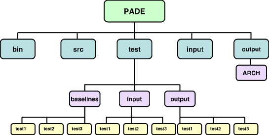
Figure 1: Schematic structure of the package

For users’ benefit we supply a file README in directory PADE. The file provides a brief summary of the code structure and basic instructions for its users.

8.3 Building PADE_II executables from source

To build the executables PADE_II and the utilities VALIDATE and TRANSMP90 (a FORTRAN -multiprecision translator) perform the following steps:

cd src

Change the definition of F77, FFLAGS, NAGPATH and LFLAGS in Makefile if necessary.

make all

This will create the binaries PADE_II, VALIDATE, and TRANSMP90 in directory PADE/bin.

To build each executable separately simply type

make exe_name

where exe_name is either PADE_II or VALIDATE or TRANSMP.

8.4 Validation tests

The input for three jobs, test1, test2 and test3, are provided in directories test/input/test_name where test_name is either test1 or test2 or test3. To submit and run a test suite, type the following commands:

cd PADE/test

./run_TEST

All tests are run in separate directories, PADE/test/output/test1, PADE/test/output/test2 and PADE/test/output/test3. Each test takes about from few seconds to several minutes to run on a reasonably modern computer. To analyse the test results, inspect the message at the conclusion of the testing process. The message

Test test_name was successful

confirms that the code passed the validation test test_name . The results of the simulation can be viewed in the output/test_name directory. The message

Your output differs from the baseline!

means that the calculated data significantly differ from that in the baselines. Check the files output/test_name/diff_file to judge the differences.

9 Running PADE_II

9.1 Computational modules

PADE_II: the code for calculating the poles and zeros, as well as the poles residues in the plane of complex angular momentum / complex energy using Padé approximation of type II.

VALIDATE: the code validating the results obtained using PADE_II.

TRANSMP: a translation program allowing for extension of the FORTRAN 77 language to multiple precision data types.

Running PADE_II involves the following steps:

1. Create the input data,

2. Specify the run options and execute PADE_II,

3. Validate the output data (optional).

9.2 Creating input data

Two input files are required for running calculations: a parameter file, param.pade, and the file containing the input data to be Padé approximated. The latter can have an arbitrary name. Examples of input files can be found in directory PADE/input.

9.3 Executing a simulation

The script run_PADE in PADE/ directory automates calculations. The following assumptions are made in the scripts:

* all binaries are placed in PADE/bin

* input files are located in directory PADE/input

* output files can be found in PADE/output on completion of the calculation.

Four options can be specified in the script run_PADE before running:

inputfile: the name of the input file. Default is input. The user has freedom in choosing a name for the input file

runoption: an option controlling a length of output. Please set runoption to production for a production run or to full_print for the detailed output (see section 6.13 for further detail). The default is production

testoption: an option allowing for a use of the test script run_TEST in PADE/test directory. Please set testoption to test for testing or leave blank otherwise. Default is a blank value.

validation: an option allowing for validating the output data using the utility validate. Please set validation to valid_yes to validate the results or to valid_no otherwise. The default is valid_yes. We encourage users to choose the default option.

We recommend running a calculation in directory PADE/. The command

../bin/run_PADE
 

immediately starts the calculation.

9.4 Output data

On completion of the calculation all output files will be redirected to PADE/output. The directory ARCH will be created automatically in PADE/output if it does not exist yet. Please take care of the output from the previous run in directory PADE/output as they will be automatically removed at the start of the next calculation. It does not apply to the content of directory ARCH. The following output files can be found on completion of the PADE_II run with the chosen runoption to be production:

out_pade contains all significant calculated data, such as zeros, poles, phase coefficients

out_pade_test contains the same data as in out_pade but in the different format: with 8 digits shown after the decimal point

resides contains the calculated resides

job.log contains PADE_II job statistics file and the summary of the validation procedure (if any)

summary.$DATE stores the name of the input file used. $DATE contains origination date and time. The file is located in PADE/output/ARCH.

If runoption is chosen to be full_print then a number (depending on parameters used) of output files will be created in directory PADE/output. Those files provide detailed information and extra control of the calculation (see 6.13).

10 Test runs

Three suitable test runs of the PADE_II program package are provided. The input and output files for these tests are included in the package.

10.1 Test 1: The hard sphere model (Regge poles)

The first test involves $S$ matrix element for potential (single channel) scattering off a hard sphere of a radius $R-d$ surrounded by a thin semi-transparent layer of a radius $R$, so that the spherically symmetric potential $V(r)$ is infinite for $r<R-d$ and $\Omega\delta(r-R)$ ($\delta(x)$ is the Dirac delta) elsewhere. The energy of a non-relativistic particle is $E=k^{2}/2$, where we have put to unity $\hbar$ as well as the particle’s mass. A detailed discussion of this model can be found in Refs.[23] and [40]. The input file $smre.test1$ contains $40$ partial waves, $J=0,1...39$, for a model with $d/R=3.5/20$, $R\Omega=50$ and $kR=20$. The input files param.pade and input_file are as follows

ipar  iprec  imult   nstime   nprint     fac
 0      1       0       1       2000   0.000001

and

        nread     niterr       shift   jstart   jfin   inv  dxl
          40           2          20       1     39    -1   1.5
  0.000000000000000E+000 -0.453586393436287      -0.891212311230866
   1.00000000000000       0.543023350525081       0.839717595852626
   2.00000000000000      -0.704041319711519      -0.710159010460940
   3.00000000000000       0.888058065387598       0.459731304677021
   4.00000000000000      -0.998289775531788      -5.845959347012353E-002
   5.00000000000000       0.890738274698926      -0.454516584940946
   6.00000000000000      -0.434473236117557       0.900684743457741
   7.00000000000000      -0.333662099368660      -0.942692740740534
   8.00000000000000       0.977155982861081       0.212523375558536
   9.00000000000000       0.720595526411046       0.693355671583052
   10.0000000000000       0.664031500188029      -0.747704598593613
   11.0000000000000       0.666737175185565       0.745292921760011
   12.0000000000000      -0.856249634342491       0.516562255384915
   13.0000000000000      -0.425006254859363      -0.905190412747737
   14.0000000000000       0.899356824643227      -0.437215395391851
   15.0000000000000       0.564958024126621       0.825119646460405
   16.0000000000000      -0.624574779169686       0.780965008963358
   17.0000000000000      -0.976521727561331      -0.215418930460241
   18.0000000000000      -0.404573635897627      -0.914505425427632
   19.0000000000000       0.324581052098112      -0.945857886058409
   20.0000000000000       0.770295446722293      -0.637687168413246
   21.0000000000000       0.944712675162273      -0.327899315930580
   22.0000000000000       0.990708814056840      -0.136000168198755
   23.0000000000000       0.998911104661369      -4.665409932903946E-002
   24.0000000000000       0.999908936584357      -1.349513018612076E-002
   25.0000000000000       0.999994360792535      -3.358330407996912E-003
   26.0000000000000       0.999999731959201      -7.321758842783459E-004
   27.0000000000000       0.999999989939087      -1.418514237449860E-004
   28.0000000000000       0.999999999695326      -2.468496879744044E-005
   29.0000000000000       0.999999999992432      -3.890541681219141E-006
   30.0000000000000       0.999999999999844      -5.590812250283133E-007
   31.0000000000000       0.999999999999997      -7.367561396623236E-008
   32.0000000000000        1.00000000000000      -8.958077930733973E-009
   33.0000000000000        1.00000000000000      -1.020177826822646E-009
   34.0000000000000        1.00000000000000      -1.241835300295753E-010
   35.0000000000000        1.00000000000000       1.384853577811148E-011
   36.0000000000000        1.00000000000000       7.957477362324928E-014
   37.0000000000000        1.00000000000000       1.036005717080183E-014
   38.0000000000000        1.00000000000000       9.917113494880074E-015
   39.0000000000000        1.00000000000000       1.000697917812276E-014

respectively. The output file out_pade contains the data which define a $[19/19]$ Padé approximant (cf.Eq.7)

          19          19
 ZEROES
           1 (39.4911990444339,6.19497800757232)
           2 (36.9799732414393,8.43963299665421)
           3 (34.0133580781357,10.7738603477704)
           4 (18.1696986797484,18.1210578980068)
           5 (12.2668387160508,19.4124385241265)
           6 (5.83305872468270,20.3995836982532)
           7 (-3.02720086016028,20.1000359128290)
           8 (24.6628733158064,2.67477729890608)
           9 (-12.0363094250139,11.9513828909703)
          10 (-12.1776119341912,1.25316966687318)
          11 (9.14176939602146,-0.234322402585798)
          12 (14.5523482093869,-1.109430235203338E-003)
          13 (21.8125711139416,-4.39732130205730)
          14 (25.1197847383941,-10.5991913301718)
          15 (26.2269224845999,-12.0435440258052)
          16 (23.6585655155745,-7.73331773608408)
          17 (24.6544987721333,-2.67109330547254)
          18 (35.7440073905768,-3.138594025574343E-003)
          19 (41.8597046798259,3.61274050690063)
 POLES
           1 (35.7440073903667,-3.138542834584743E-003)
           2 (24.6628733369383,2.67477729572751)
           3 (23.6585655606588,7.73331699080323)
           4 (26.2268330879602,12.0434263955026)
           5 (25.1197975398861,10.5992368004622)
           6 (21.8125711134792,4.39732130283915)
           7 (14.5523482093869,-1.109430235909550E-003)
           8 (9.14176939602135,0.234322402586938)
           9 (-12.1774051901505,-1.25342226018641)
          10 (-12.0359449939580,-11.9511561142494)
          11 (24.6544987511749,-2.67109330818693)
          12 (-3.02710863601014,-20.0995263248157)
          13 (5.83307474171240,-20.3992358761048)
          14 (12.2668862760970,-19.4121731020176)
          15 (18.1697778070471,-18.1208548568950)
          16 (34.0131260419783,-10.7739117218385)
          17 (36.9796907970374,-8.43956124986996)
          18 (39.4909636463193,-6.19477828169534)
          19 (41.8595888739847,-3.61248175364997)
 PHASE COEFF a+b*J+c*J^2
   2.67555460298088        2.73887621121985      -4.727964256522786E-002
 CONST FACTOR K_n
 (0.357477628915536,0.933794075548949)
 PARITY CHANGE FROM ORIGINAL DATA
           0

Figure 2 shows the behaviour of the Padé approximant along the real $J$ axis. The pole/zero configuration of the $[19/19]$ Padé approximant is shown in Fig. 3a.

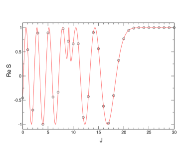
Figure 2: Real parts of the input values of the hard-sphere model matrix element $S(E,J)$, $J=0,1,...39$ (circles) and the real part of the $[19/19]$ Padé approximant constructed from these values (solid).

Figure 3b shows the results of two similar calculations ($nstime=2$ chosen in the input param.pade ) . However, in each calculation a random noise with the noise factor in Eq.(10) $fac=10^{-6}$ has been added to the input data. As discussed in Sect.2, additional contamination with a non-analytical noise results in squeezing of the domain of validity of an approximant as well as in production of additional Froissart doubles close to the real axis.

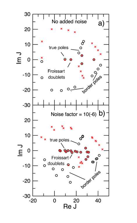
Figure 3: a) Positions of poles (circles) and zeros (crosses) in the complex angular momentum plane for the hard-sphere model. Three types of poles are indicated. The true poles include an isolated resonance with $ReJ\approx 10$ on a metastable state trapped between the core and the outer layer as well as the first four poles of the infinite sequence corresponding to diffraction on the outer layer [23]. There are also several Froissart doublets. Remaining poles and zeroes mark a boundary beyond which the approximant fails, b) Poles and zeroes of two $[19/19]$ Padé approximants constructed from the same input values, but contaminated with random noise with $fac=10^{-6}$.

10.2 Test 2: The hard sphere model (complex energy poles)

For the second test the input file $smrj.test2$ contains $49$ values of $S(E,J=10)$ on the equidistant energy grid $200\leq R^{2}E_{j}=R^{2}k_{j}^{2}/2<250$ for the same model with $d/R=3.5/20$, $R\Omega=50$. The input files param.pade and input_file are as follows

ipar  iprec  imult    nstime  nprint      fac
 0      0       0       0      2000   0.000001

and

nread niter    shift    jstart     jfin    inv dxl
  50     5       225.       1        49    -1  1.5
   200.000000000000       0.664031500188029      -0.747704598593613
   201.000000000000       0.640154019051953      -0.768246595756617
   202.000000000000       0.624758751680046      -0.780817841880672
   203.000000000000       0.621472411367862      -0.783436048384688
   204.000000000000       0.635123092357332      -0.772410938266969
   205.000000000000       0.671965187035159      -0.740582735022093
   206.000000000000       0.739032006430064      -0.673670315118571
   207.000000000000       0.839572088290516      -0.543248293659080
   208.000000000000       0.954602056895436      -0.297884059612129
   209.000000000000       0.992695675238598       0.120645332949871
   210.000000000000       0.761692689904593       0.647938458610000
   211.000000000000       0.223560893654405       0.974689964464827
   212.000000000000      -0.304719743630442       0.952442060096988
   213.000000000000      -0.627460687663612       0.778648242428316
   214.000000000000      -0.789516598726692       0.613729207660053
   215.000000000000      -0.866908960431839       0.498466502709047
   216.000000000000      -0.903313320122455       0.428981404829331
   217.000000000000      -0.919143298112510       0.393923339667577
   218.000000000000      -0.923506334424972       0.383583172567504
   219.000000000000      -0.920433057855924       0.390900225129116
   220.000000000000      -0.911688160524598       0.410882827530277
   221.000000000000      -0.898018594051828       0.439957503330923
   222.000000000000      -0.879718432979564       0.475494982808420
   223.000000000000      -0.856891241732639       0.515497235532739
   224.000000000000      -0.829574633076335       0.558395852560049
   225.000000000000      -0.797800024420750       0.602922151719648
   226.000000000000      -0.761621008213086       0.648022715534326
   227.000000000000      -0.721126129965770       0.692803799556982
   228.000000000000      -0.676443760254596       0.736494290006801:
   229.000000000000      -0.627742897353397       0.778420744085332
   230.000000000000      -0.575231856010094       0.817990410598549
   231.000000000000      -0.519155855614356       0.854679587670915
   232.000000000000      -0.459794039256912       0.888025586041198
   233.000000000000      -0.397456205017629       0.917621144641396
   234.000000000000      -0.332479399617643       0.943110517823808
   235.000000000000      -0.265224455432244       0.964186697813587
   236.000000000000      -0.196072515839709       0.980589398541656
   237.000000000000      -0.125421575098095       0.992103537187482
   238.000000000000      -5.368304983650439E-002  0.998558025434802
   239.000000000000       1.872160509145225E-002  0.999824735392559
   240.000000000000       9.136422532965484E-002  0.995817542690383
   241.000000000000       0.163813199773938       0.986491376333227
   242.000000000000       0.235636656616718       0.971841224716515
   243.000000000000       0.306405561742876       0.951901061945533
   244.000000000000       0.375696718367498       0.926742669681230
   245.000000000000       0.443095656457025       0.896474338299161
   246.000000000000       0.508199400868439       0.861239437646094
   247.000000000000       0.570619106928023       0.821214853012697
   248.000000000000       0.629982552997152       0.776609285882670
   249.000000000000       0.685936479728164       0.727661422488601
   250.000000000000       0.738148766653856       0.674637975722825
   10.5000000000000        20.0000000000000        3.50000000000000
   5.00000000000000       0.000000000000000E+000
   

respectively. The output file out_pade contains the data which defines a $[24/24]$ Padé approximant (cf.Eq.9)

          24          24
 ZEROES
           1 (268.545717720799,11.4671502976118)
           2 (261.728173386068,19.6753217953572)
           3 (254.557738718419,26.5701017472017)
           4 (245.881831513906,33.4912944344641)
           5 (232.951306941574,1.877662435186347E-004)
           6 (224.121052772429,4.19191611872841)
           7 (220.411919658935,1.15434928347258)
           8 (217.652385494978,2.852399491808721E-002)
           9 (210.331899212664,2.72550066138290)
          10 (209.654815139940,2.641960499678558E-004)
          11 (212.868385932177,3.598159766224907E-004)
          12 (186.524319063303,-9.14781503752908)
          13 (206.326496566314,1.959778648327130E-004)
          14 (192.395056901391,-15.3604166393560)
          15 (198.447273067597,-20.3445869086093)
          16 (205.051304571580,-24.9792759962048)
          17 (212.514236963499,-29.6992072722432)
          18 (221.649194114141,-34.9881538867756)
          19 (220.510303177377,-1.14210693606552)
          20 (224.031598890991,-4.30241298271368)
          21 (226.023976865667,2.261727493434314E-002)
          22 (238.490995343524,-1.47246931619824)
          23 (242.730754962705,-3.477317333857598E-004)
          24 (238.491169699397,1.46793956930393)
 POLES
           1 (242.730754962705,-3.477317319122845E-004)
           2 (238.491169699401,1.46793956929681)
           3 (226.023976865667,2.261727493435679E-002)
           4 (224.121052772959,4.19191611897241)
           5 (220.411919658902,1.15434928347629)
           6 (221.648098623382,34.9885968283023)
           7 (212.513501359997,29.7001476182166)
           8 (205.051076178872,24.9802350950195)
           9 (198.447298402548,20.3453065442821)
          10 (192.395118933229,15.3609323651784)
          11 (206.326496566310,1.959780792806160E-004)
          12 (186.524346342521,9.14822455412355)
          13 (212.868385932166,3.598159852993832E-004)
          14 (209.654815139977,2.641956005816340E-004)
          15 (210.331899212667,-2.72550066136285)
          16 (217.652385494976,2.852399491882152E-002)
          17 (220.510303177407,-1.14210693605598)
          18 (224.031598890383,-4.30241298239934)
          19 (232.951306941574,1.877662434131332E-004)
          20 (245.882621687043,-33.4918893250634)
          21 (254.558185226003,-26.5708559777491)
          22 (261.728380822961,-19.6760176672578)
          23 (268.545803872059,-11.4677538269500)
          24 (238.490995343520,-1.47246931620535)
 PHASE COEFF a+b*J+c*J^2
  -283.165777224028        2.47637834572351      -5.407538683988272E-003
 CONST FACTOR K_n
 (0.908740385440017,0.417744816017221)
 PARITY CHANGE FROM ORIGINAL DATA
           0
 

Figure 4 shows the behaviour of the Padé approximant along the real $E$-axis. The pole/zero configuration of the $[24/24]$ Padé approximant is shown in Fig. 5.

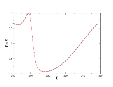
Figure 4: Real parts of $S(E_{m},J=10)$, $m=1,...49$ (circles) and the $[24/24]$ Padé approximant constructed from these values (solid).

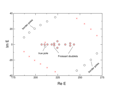
Figure 5: Positions of poles (circles) and zeros (crosses) in the complex energy plane for 10-th partial wave ($J=10$) of the hard-sphere model. Three types of poles are indicated. The true pole with $ReE\approx 212$ corresponds to a metastable state trapped between the core and the outer layer. There are also several Froissart doublets. Remaining poles and zeroes mark a boundary beyond which the approximant fails.

10.3 Test 3: Multiple precision (Regge poles)

The third test, whose purpose is to illustrate the use of the multiple precision option, involves constructing a Padé approximant for the inelastic matrix element for the $He^{+}-Ne$ inelastic collision model of Olson and Smith [53] computed by K.Thylwe [54]. The input consists of $111$ partial waves, i.e., the values of $S_{01}(E,J)$, $J=0,1,...,110$ at a fixed value of the collision energy. The input file param.pade is

ipar  iprec  imult    nstime  nprint      fac
 0      1       1      0        2000   0.000001

and the input input_file together with the output out_pade, too long to be printed here, are supplied with the code. The number of input data is such that a double precision calculation (choosing ’imult’$=0$ in param.pade) produces incorrect Padé approximant which fails to reproduce the input values (Fig.6a). A calculation with a multiple precision of $60$ digits yields the correct approximant (Fig.6b). In general, it is recommended to repeat a DP calculation with a choice of a higher precision, in order to see if this changes the computed approximant in any significant way.

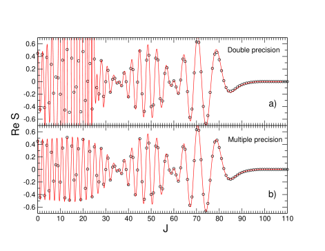
Figure 6: Real parts of $S(E_{m},J=10)$, $m=1,...49$ (circles) and the $[55/55]$ Padé approximant constructed from these values (solid).

References

- [1] S. A. Harich, D. X. Dai, C. C. Wang, X. Yang, S. D. Chao and R. T. Skodje, Forward scattering due to slow-down of the intermediate in the H+HDD+H2 reaction, Nature, 419, (2002) 281.
- [2] D. C. Clary, Quantum Theory of Reaction Dynamics, Science, 279 (1998) 1879.
- [3] D. Skouteris, D. E. Manolopoulos, W. Bian, H-J Werner, L-H Lai and K. Liu, Van der Waals Interactions in the Cl + HD Reaction, Science, 286 (1999) 1713.
- [4] P. Casavecchia, N Balucani and G. G. Volpi, Cross beam studies of reaction dynamics, Ann. Rev. Phys. Chem., 50 (1999) 347.
- [5] W. H. Miller, Adv. Chem. Phys., Classical-Limit Quantum Mechanics and the Theory of Molecular Collisions, 25 69 (1974) 69.
- [6] D. Skouteris, J. F. Castillo and D. E. Manolopoulos, ABC: a quantum reactive scattering problem, Comp. Phys. Commun, 133 (2000) 128.
- [7] S. C. Althorpe, F. Fernández-Alonso, B. D. Bean, J. D. Ayers, A. E. Pomerantz, R. N. Zare and E. Wrede, Observation and interpretation of a time-delayed mechanism in hydrogen exchange reaction, Nature, 416 (2002) 67.
- [8] V. Aquilanti, S. Cavalli and D. De Fazio, Hyperquantization algorithm. I. Theory for triatomic systems, J. Chem. Phys., 109 (1998) 3792.
- [9] V. Aquilanti, S. Cavalli, D. De Fazio, A. Volpi, A. Aguilar, X. Giménez and J. F. Lucas, Exact reaction dynamics by the hyperquantization algorithm: integral and differential cross sections for F + H2, including long-range and spin-orbit effects, Phys. Chem. Chem. Phys., 4, 401 (2002).
- [10] It is worth noting that the applications usually require the knowledge of only a few leading true pole positions and residues. The remaining poles and zeroes of the approximant are then used to reproduce the direct part of the -matrix element on the real axis, which is independent of their individual positions and residues.
- [11] J.N.L. Connor, Molecular collisions and the semiclassical approximation, Meldola Medal Lecture, Chemical Society Reviews,5, (1976), 125.
- [12] J.N.L. Connor, W. Jakubetz and C.V. Sukumar, Exact quantum and semiclassical calculation of the positions and residues of Regge poles for interatomic potentials, J. Phys. B, 9, (1976), 1783.
- [13] J.N.L. Connor and W. Jakubetz, Rainbow scattering in atomic collisions: A Regge pole analysis, Mol. Phys., 35, (1978) 949.
- [14] J.N.L. Connor, D.C. Mackay and C.V. Sukumar, Quantum and semiclassical calculation of Regge pole positions and residues for complex optical potentials, J. Phys. B, 12, (1979), L5151.
- [15] J.N.L.Connor, Semiclassical theory of elastic scattering, in ”Semiclassical methods in molecular scattering and spectroscopy.” Proceedings of the NATO Advanced Study Institute held in Cambridge, England, in September, 1979. Edited by M.S. Child. Reidel, Dordrecht, The Netherlands, (1980) 45.
- [16] J.N.L. Connor, D. Farrelly and D.C. Mackay, Complex angular momentum analysis of diffraction scattering in atomic collisions, J. Chem. Phys., 74, (1981) 3278.
- [17] K-E. Thylwe and J.N.L. Connor, A complex angular momentum theory of modified Coulomb scattering, J. Phys. A, 18, (1985), 2957.
- [18] J.N.L. Connor, D.C. Mackay and K-E. Thylwe, Computational study and complex angular momentum analysis of elastic scattering for complex optical potentials, J.Chem. Phys., 85, (1986) 6368.
- [19] J.N.L. Connor and K-E. Thylwe, Theory of large angle elastic differential cross sections for complex optical potentials: Semiclassical calculations using partial waves, l-windows, saddles and poles, J.Chem. Phys., 86, (1987) 188.
- [20] J.N.L.Connor, New theoretical methods for molecular collisions: The complex angular momentum approach, J. Chem. Soc., Faraday Transactions, 86, (1990) 1627.
- [21] P. McCabe, J.N.L. Connor and K-E. Thylwe, Complex angular momentum theory of molecular collisions: New phase rules for rotationally inelastic diffraction scattering in atom homonuclear-molecule collisions, J.Chem. Phys., 98, (1993) 2947.
- [22] D.M. Brink, Semi-classical Methods in Nucleus-Nucleus Scattering, Cambridge University Press, Cambridge, 1985.
- [23] D. Sokolovski and A. Z. Msezane, Semiclassical complex angular momentum theory and Padé reconstruction for resonances, rainbows, and reaction thresholds, Phys. Rev. A., 70 (2004) 032710.
- [24] D. Vrinceanu, A. Z. Msezane, D. Bessis, J. N. L. Connor and D. Sokolovski, Chem. Phys. Lett., Padé reconstruction of Regge poles from scattering matrix data for chemical reactions, 324 (2000) 311.
- [25] D. Sokolovski, S. Sen, On the type II Padé reconstruction of a scattering matrix element, Semiclassical and other Methods for Understanding Molecular Collisions and Chemical reactions, Collaborative Computational Project on Molecular Quantum Dynamics (CCP6), Daresbury, UK, (2005) 104.
- [26] D. Sokolovski, J. N. L. Connor and G. C. Schatz, New uniform semiclassical theory of resonance angular scattering for reactive molecular collisions, Chem. Phys. Lett., 238 (1995) 127.
- [27] D. Sokolovski, J. N. L. Connor and G. C. Schatz, Complex angular momentum analysis of resonance scattering in the Cl + HCl ClH + Cl reaction, J. Chem. Phys., 103 (1995) 5979.
- [28] D. Sokolovski, J. F. Castillo and C. Tully, Semiclassical angular scattering in the F + H2 HF + H reaction: Regge pole analysis using the Padé approximation, Chem. Phys. Lett., 313 (1999) 225.
- [29] D. Sokolovski, J. F. Castillo, Differential cross sections and Regge trajectories for the F + H2 HF + H reaction, 2 (2000) 507.
- [30] D. Sokolovski, S.K.Sen, V.Aquilanti, S.Cavalli and D.De Fazio, Interacting resonances in the F + H2 reaction revisited: Complex terms, Riemann surfaces, and angular distributions J. Chem. Phys., 126 (2007) 084305.
- [31] D. Sokolovski, D.De Fazio, S.Cavalli and V.Aquilanti, Overlapping resonances and Regge oscillations in the state-to-state integral cross sections of the F + H2 reaction, J. Chem. Phys., 126 (2007) 12110.
- [32] D. Sokolovski, D.De Fazio, S.Cavalli and V.Aquilanti, On the origin of the forward peak and backward oscillations in the the F + H2(v=0) HF(v’=2) + H reaction, Phys.Chem.Chem.Phys., 9 (2007) 1.
- [33] F. J. Aoiz, L. Bañares, J. F. Castillo and D. Sokolovski, Energy dependence of forward scattering in the differential cross section of the H + D2 HD() + D reaction, J. Chem. Phys., 117 (2002) 2546.
- [34] D. Sokolovski, Glory and thresholds effects in H + D2 reactive angular scattering, Chem. Phys. Lett., 370 (2003) 805.
- [35] D. Sokolovski, Complex-angular-momentum analysis of atom-diatom angular scattering: Zeros and poles of the S matrix, Phys. Rev. A., 62 (2000) 024702-01.
- [36] D. Sokolovski, A.Z. Msezane, Z. Felfli, S.Yu. Ovchinnikov and J.H. Macek, What can one do with Regge poles?, Nuclear Instruments and Methods in Physics Research Section B: Beam Interactions with Materials and Atoms, Volume 261, (2007)133.
- [37] A.J. Totenhofer, C. Noli and J.N.L. Connor, Dynamics of the I + HI IH + I reaction: Application of nearside-farside, local angular momentum and resummation theories using the Fuller and Hatchell decompositions, Physical Chemistry Chemical Physics, 12,(2010), in print.
- [38] J. H. Macek, P. S. Krstic, and S. Yu. Ovchinnikov, Regge Oscillations in Integral Cross Sections for Proton Impact on Atomic Hydrogen, Phys. Rev. Lett. 93, (2004) 183203.
- [39] D. Sokolovski, D.De Fazio, S.Cavalli and V.Aquilanti, Overlapping resonances and Regge oscillations in the state-to-state integral cross sections of the F + H2 reaction, J. Chem. Phys., 126 (2007) 121101.
- [40] D. Sokolovski, Complex-angular-momentum (CAM) route to reactive scattering resonances: from a simple model to the F + H2 HF + H reaction , Phys. Scr., 78 (2008) 058118.
- [41] P. G. Burke and C. Tate, A program for calculating Regge trajectories in potential scattering, Comput. Phys. Commun. 1, 1969, 97.
- [42] D. Sokolovski, Z. Felfli, S. Yu. Ovchinnikov, J. H. Macek, and A. Z. Msezane, Regge oscillations in electron-atom elastic cross sections, Phys. Rev. A 76,(2007) 012705.
- [43] D. Bessis, A. Haffad, and A. Z. Msezane, Momentum-transfer dispersion relations for electron-atom cross sections, Phys. Rev. A., 49 (1994) 3366.
- [44] G. A. Baker, Jr., The essentials of Padé Approximations, Academic, New York, 1975.
- [45] M.S. Petkovic, C.Carstensen. and M. Trajkovic, Weierstrass formula and zero-finding methods, Numerische Mathematik, 69: (1995).
- [46] D. H. Bailey, Algorithm 719, ”Multiprecision translation and execution of Fortran programs”. ACM Transactions on Mathematical Software, 19(3):288 (1993).
- [47] S. Sokolovski, J. N. L. Connor, Semoclassical nearside-farside theory for inelastic and reactive atom-diatom collisions, Chem. Phys. Lett., 305 (1999) 238.
- [48] W. Gautschi, in Handbook of Mathematical Functions, edited by M. Abramowitz and I. A. Stegun (Harri Deutsch, Htun, 1984).
- [49] J. N. L. Connor, J. Chem. Soc. Faraday Trans., 305 (1990) 1627.
- [50] Numerical Algorithms Group, Fortran Library Manual, Mark 19, subroutine G05CAF (NAG, OXFORD, 2002).
- [51] Numerical Algorithms Group, Fortran Library Manual, Mark 21, subroutine C02AFF (NAG, OXFORD, 2004).
- [52] Numerical Algorithms Group, Fortran Library Manual, Mark 21, subroutine E02ACF (NAG, OXFORD, 2004).
- [53] R.E. Olson and F.T.Smith Phys. Rev. A. 3, (1971) 1607; Erratum, Phys. Rev. A. 6, (1972) 526.
- [54] K.-E. Thylwe (to be published).