Variational Heteroscedastic Volatility Model

Abstract

We propose Variational Heteroscedastic Volatility Model (VHVM) - an end-to-end neural network architecture capable of modelling heteroscedastic behaviour in multivariate financial time series. VHVM leverages recent advances in several areas of deep learning, namely sequential modelling and representation learning, to model complex temporal dynamics between different asset returns. At its core, VHVM consists of a variational autoencoder to capture relationships between assets, and a recurrent neural network to model the time-evolution of these dependencies. The outputs of VHVM are time-varying conditional volatilities in the form of covariance matrices. We demonstrate the effectiveness of VHVM against existing methods such as Generalised AutoRegressive Conditional Heteroscedasticity (GARCH) and Stochastic Volatility (SV) models on a wide range of multivariate foreign currency (FX) datasets.

C32, C45, C53,

1 Introduction

Financial time series is known to exhibit heteroscedastic behaviour - time-varying conditional volatility (Engle and Patton, 2007; Poon and Granger, 2003). Being able to model and predict this behaviour is of practical importance to professionals in finance for the purpose of risk management (Christoffersen and Diebold, 2000; Long et al., 2020), derivative pricing (J.Duan, 1995), and portfolio optimisation (Ranković et al., 2016; Escobar-Anel et al., 2022).

It is well documented in literature that (conditional) volatility is forecastable on hourly or daily frequencies (Christoffersen and Diebold, 2000). On a univariate level, this involves predicting time-varying variances of asset returns; this predictability can be attributed to the so-called volatility clustering phenomenon: large (small) changes in asset price are often followed by further large(small) changes (Engle and Patton, 2007; Fama, 1965; Schwert, 1989). On a multivariate level (involving a portfolio of assets), volatility forecasting involves estimating conditional covariances between asset pairs in addition to conditional variances of the assets. One could argue that some of this predictability comes from the so-called spillover effect: the transfer of shock between different financial markets (Jebran et al., 2017; Hassan and Malik, 2007; Du et al., 2011). An effective multivariate volatility model therefore needs to capture both intra and inter-time series dynamics.

Traditional volatility forecasting models can be divided into two main categories: Generalised AutoRegressive Conditional Hertoscedasitcity (GARCH) (Bollerslev, 1986; Nelson, 1991; Glosten et al., 1993) and Stochastic Volatility (SV) (Jacouier et al., 1994; Chan and Grant, 2016) models. The two competing classes of models rely on different underlying assumptions (Luo et al., 2018). GARCH models describe a deterministic relationship between future conditional volatility and past conditional volatility and squared returns. SV models assumes that conditional volatility follows a latent autoregressive process. Although there is no general consensus that GARCH is always superior to SV (or vice versa), there is some evidence that SV models are more flexible in modelling the characteristics of asset returns (Chan and Grant, 2016; Shapovalova, 2021). Nonetheless, the popularity of GARCH models seems to surpass that of SV models due to several reasons. Firstly, GARCH models are easier to fit than SV models. The parameters of GARCH are obtained using maximum likelihood estimation, whereas for SV models one needs to obtain samples from an intractible posterior distribution using methods such as Markov chain Monte Carlo (MCMC), which works well when the number of parameters is small, however the convergence can be slow in larger models (Shapovalova, 2021). Secondly, there is an abundance of open-source software (packages) for GARCH models, such as fGarch (Wuertz et al., 2017) and rugarch (Galanos and Kley, 2022) in the programming language R, and arch (Sheppard et al., 2022) in Python. For SV models however, there was no go-to package for model estimation until the release of stochvol and factorstochvol (Hosszejni and Kastner, 2021) in R.

It is worth mentioning that GARCH models too suffer from the curse of dimensionality. For a portfolio of $n$ assets, the computational complexity of GARCH models scales with $O(n^{5})$, which makes it impossible fit to beyond a portfolio of roughly 5 assets (Wu et al., 2013).

In recent years, the application of deep learning models for time series forecasting has achieved state of the art performances in many domains (Bandara et al., 2019; Böse et al., 2017; Li et al., 2018). Since our observations consist of multiple asset returns time series, a natural research direction would be to investigate whether deep learning models can capture complex dependencies between different assets across time. There are two main obstacles in this task. Firstly, the conditional volatility (covariance matrix) is a latent variable and must be inferred using observational data (Luo et al., 2018). Secondly, for a matrix to be a valid covariance matrix, it must be symmetric and positive definite (Engle and Kroner, 1995). How to impose these constraints on a neural network such that its outputs are valid covariance matrices is a challenging task.

To tackle the first challenge, we adopt a recent trend that combines a variational autoencoder (VAE) and a recurrent neural network (RNN) (a VRNN) to allow efficient structured inference over a sequence of continuous latent random variables (Chung et al., 2015; Bayer and Osendorfer, 2014; Krishnan et al., 2017; Fabius and van Amersfoort, 2015; Fraccaro et al., 2016; Karl et al., 2017). The use of a VAE (and hence variational inference) translates posterior approximation into an optimisation task which can be solved using a neural network trained with stochastic gradient descent. The use of an RNN allows information from previous steps to be used in the modelling and forecasting of the latent variable in future steps. In fact, this promising framework has been explored in Yin and Barucca (2022) and Luo et al. (2018). In Yin and Barucca (2022), the authors proposed a neural network adaptation of the GARCH model which showed improved performance over traditional GARCH models. However, this model also suffers from the curse of dimensionality as it is still a GARCH model by design. Since the focus of this paper is on multivariate volatility, not being able to scale up to higher dimensions (beyond at least 5) is a big limitation. The authors in Luo et al. (2018) proposed a purely data driven approach to volatility forecasting under the VRNN framework which we used as a baseline model in our results section.

To tackle the second challenge, one possible approach is to combine traditional econometrics models with deep learning models. Traditional econometrics models have well understood statistical properties and neural networks can be used to enhance the predictive power of the model. In Yin and Barucca (2022), the authors use a neural network to parameterise the time-varying coefficients of the BEKK(1,1) model, which is a multivariate GARCH model proposed by Engle and Kroner (1995). The BEKK model produces symmetric and positive definite covariance matrices by design and therefore no other constraints need to be applied to the neural network output. As mentioned previously however, many econometric models suffer from curse of dimensionality. Instead, we follow the approach in Dorta et al. (2018) and design our neural network such that it outputs the Cholesky decomposition of the precision matrix (inverse of the covariance matrix) at every time step. We will show later on how this guarantees symmetry and positive definiteness. (Engle and Kroner, 1995)

Our main contribution is therefore an end-to-end neural network architecture capable of forecasting valid covariance matrices. We show in the results section that VHVM consistently outperforms existing GARCH and SV baselines on a range of multivariate FX portfolios.

The rest of the paper is structured as follows: in section 2 we present a summary of the field of volatility forecasting and introduce some of the popular models; also discuss how they are related to our proposed model. In section 3 we formally introduce VHVM: its generative and inference components, and model training and forecasting. In section 4 we outline the experiments and data used to show the effectiveness of VHVM against existing baselines from both traditional econometrics and the field of deep learning.

2 Related Work

For a financial asset with price $S_{t}$ at time $t$, its log returns are computed as $r_{t}=log(S_{t})-log(S_{t-1})$. The returns process $r_{t}$ can be assumed to have a conditional mean $\mathbb{E}[r_{t}|\emph{I}_{t-1}]=0$ and a conditional variance $\mathbb{E}[{r_{t}}^{2}|\emph{I}_{t-1}]={\sigma_{t}}^{2}$, in other words $r_{t}|\emph{I}_{t-1}\sim\mathcal{N}(0,\sigma_{t}^{2})$. The information set $\emph{I}_{t}$ describes all relevant available at time $t$: $\emph{I}_{t}=\{r_{1:t},{\sigma_{1:t}}^{2}\}$. The time variation of conditional variance $\sigma$ is known as heteroscedasticity and the aim of volatility forecasting is to model this behaviour (Engle and Kroner, 1995).

2.1 Generalise Autoregressive Conditional Heteroscedasticity

ARCH (Engle, 1982) and GARCH (Bollerslev, 1986) models have been dominating the field of volatility forecasting since the late 1900s due to their simple model form, explainability, and ease of estimation. Many GARCH model variants have since been proposed to account for well-known stylised facts about financial time series such as volatility clustering and leverage effect (Engle and Patton, 2007). The EGARCH (Nelson, 1991) and GJR-GARCH (Glosten et al., 1993) models for example, were designed to specifically accommodate the leverage effect. The most general GARCH($p$,$q$) model proposed by Bollerslev (1986) describes a deterministic relationship between future conditional volatility, past conditional volatility and squared returns:

$$\sigma_{t}^{2}=\omega+\sum_{i=1}^{p}\alpha_{i}r_{t-i}^{2}+\sum_{j=1}^{q}\beta_{j}\sigma_{t-j}^{2},$$ (1)

where $p$ and $q$ are lag orders of the ARCH and GARCH terms, under which the returns process $r_{t}$ has an unconditional mean $\mathbb{E}[r_{t}]=0$ and unconditional variance $\mathbb{E}[r_{t}^{2}]=\frac{\omega}{1-\alpha-\beta}$.

In total, there are many hundreds of GARCH model variants, however there exists little consensus on when to use which GARCH models as their performances tend to vary with the nature and behaviour of the time series being modelled, for example, the leverage effect is frequently observed in stock returns but rarely seen in foreign exchange currency returns (Engle and Patton, 2007). In Hansen and Lunde (2005) the authors compared the performances of 330 GARCH variants on Deutsche Mark-US Dollar exchange rates and IBM returns and found that the GARCH(1,1) was not outperformed by any other model in the foreign exchange analysis. In the IBM stock returns analysis however, the authors found that GARCH(1,1) was inferior to models that explicitly accounted for the leverage effect. It has thus become common practice to explore various GARCH variants for the same task (Chan and Grant, 2016; Chu et al., 2017; Malik, 2005).

For a portfolio of assets, models tend to be multivariate generalisations of the univariate GARCH model. In additional to modelling conditional variances for each asset, one also needs to model time varying covariances between different asset pairs. The output for a multivariate GARCH model is a time-varying covariance matrix which describes the instantaneous intra and inter-asset relationships. Notable examples of multivariate GARCH models include the VEC model (Bollerslev et al., 1988), the BEKK model (Engle and Kroner, 1995), the GO-GARCH model (Van Der Weide, 2002), and the DCC-GARCH model (Christodoulakis and Satchell, 2002; Tse and Tsui, 2002; Engle, 2002). For our analysis, we used the DCC-GARCH (dynamic conditional correlation) model as a multivariate GARCH baseline. The key difference between DCC-GARCH and BEKK (a popular multivariate GARCH) is that BEKK assumes constant conditional correlation between assets, i.e. the change in the covariance between two assets with time is due to the changes in the two variances (but the conditional correlation is constant) (Huang et al., 2010). The constant conditional correlation (CCC) assumption is rather crude since during different market regimes one would expect the correlation between assets to vary. The DCC-GARCH is a generalisation of a CCC-GARCH that accounts for dynamic correlation. During the estimation procedure, various univariate GARCH models are fit for the assets, followed by estimations of the parameters for conditional correlation.

When fitting a multivariate GARCH model under the assumption of normal innovations ($\boldsymbol{r}_{t}\sim\mathcal{N}(0,\boldsymbol{\Sigma}_{t})$), we seek to maximise the multivariate normal log likelihood function (Bauwens et al., 2006):

$$\mathcal{L}(\theta)=-\frac{1}{2}\sum_{t=1}^{T}(log|\boldsymbol{\Sigma}_{t}|+\boldsymbol{r}_{t}^{T}\boldsymbol{\Sigma}_{t}^{-1}\boldsymbol{r}_{t}),$$ (2)

which becomes computationally expensive in higher dimensions since we are required (for a portfolio of $n$ assets) to invert an $n\times n$ covariance matrix $\boldsymbol{\Sigma}_{t}$ for every time step. One solution to alleviate this burden is to directly work with the precision matrix (inverse covariance matrix) instead: $\boldsymbol{P}=\boldsymbol{\Sigma}^{-1}$. Setting a neural network output to be a precision matrix rather than a covariance matrix allows us to compute the log likelihood straightaway; hence bypassing the expensive matrix inversion step during model training. When the actual covariance matrix is required during the testing phase, one could simply invert the precision matrix to obtain the covariance matrix (Luo et al., 2018; Dorta et al., 2018).

2.2 Stochastic Volatility

Stochastic Volatility is an alternative class of models that rely on assumption that the log conditional variance follows a non-deterministic autoregressive AR($p$) (usually $p=1$) process (Shapovalova, 2021):

$$ln\sigma_{t+1}^{2}=\mu+\phi ln\sigma_{t}^{2}+\sigma_{\eta}\eta_{t+1},$$ (3)

where $\eta_{t}\sim N(0,1)$ describes the innovation of the log variance process. For the rest of the section we refer the log volatility $ln\sigma_{t}^{2}$ as $h_{t}$ such that $r_{t}=exp(h_{t}/2)\epsilon_{t}$ where $\epsilon_{t}\sim N(0,1)$.

In a multivariate setting, we seek to simultaneously model the volatility movements of a group of assets (Platanioti et al., 2005). Related movements between different asset classes, financial markets or exchange rates are often observed due to them being infuenced by common unobserved drivers (or factors) (Aydemir, 1998). Diebold and Nerlove (1989) investigated the behaviour of seven dollar exchange rates for a period of 12 years and found that the seven series showed similarities in volatility behaviour in response to actions taken by the US government such as intervention efforts. Since stochastic volatility models are defined in terms of the log volatility process, it is harder to generalise a univariate model to its multivariate counterpart than a GARCH model (Platanioti et al., 2005).

In this paper we take as baseline the factor model independently proposed by Pitt and Shephard (1999) and Aguilar and West (2000). An open-source package (factorstochvol) was developed in the programming language R by Hosszejni and Kastner (2021) which we used to run the baseline SV model in our analysis. The factor volatility model (Hosszejni and Kastner, 2021) for a portfolio of $n$ assets assumes $m$ latent common factors where $m<n$. We have that:

$$\boldsymbol{r}_{t}|\boldsymbol{f}_{t}\sim\mathcal{N}(\boldsymbol{\Lambda}\boldsymbol{f}_{t},\bar{\boldsymbol{\Sigma}}_{t}),$$ (4)

$$\boldsymbol{f}_{t}\sim\mathcal{N}(0,\check{\boldsymbol{\Sigma}}_{t}),$$

where $\boldsymbol{f}_{t}=(f_{t1},...,f_{tm})^{T}$ is the vector of $m$ factors, $\boldsymbol{\Lambda}\in\mathbf{R}^{n\times m}$ is a matrix of factor loadings. The covariance matrices $\bar{\boldsymbol{\Sigma}}_{t}$ and $\check{\boldsymbol{\Sigma}}_{t}$ are diagonal and are defined as:

$$\bar{\boldsymbol{\Sigma}}_{t}=diag(exp(\bar{h}_{t1}),...,exp(\bar{h}_{tn})),$$ (5)

$$\check{\boldsymbol{\Sigma}}_{t}=diag(exp(\check{h}_{t1}),...,exp(\check{h}_{tm})),$$

where $\bar{h}$ and $\check{h}$ are the log variances of the $n$ assets and $m$ latent factors defined as follows (the AR(1) process given in (3)):

$$\bar{h}_{ti}\sim\mathcal{N}(\bar{\mu}_{i}+\bar{\phi}_{i}(\bar{h}_{t-1,i}),\bar{\sigma}_{i}^{2}),i=1,...,n,$$ (6)

$$\check{h}_{tj}\sim\mathcal{N}(\check{\mu}_{j}+\bar{\phi}_{j}(\check{h}_{t-1,j}),\check{\sigma}_{j}^{2}),j=1,...,m.$$

Given the above, the multivariate returns process follows a 0 mean multivariate normal distribution with $\boldsymbol{r}_{t}\sim\mathcal{N}(0,\boldsymbol{\Sigma}_{t})$, where $\boldsymbol{\Sigma}_{t}=\boldsymbol{\Lambda}\check{\boldsymbol{\Sigma}}_{t}\boldsymbol{\Lambda}^{T}+\bar{\boldsymbol{\Sigma}}_{t}$. We see that the factor volatility model in (4) is by nature a state space model with a random walk latent transition process and a linear emission process $\boldsymbol{r}_{t}|\boldsymbol{f}_{t}$. We will show later on that our end-to-end neural network architecture follows the same theoretical framework: a neural network (an RNN) that models the non-linear latent transition process $\boldsymbol{f}_{t}|\boldsymbol{f}_{t-1}$, a neural network (VAE) that infers the latent factors from observational data $\boldsymbol{f}_{t}|\boldsymbol{r}_{1:t}$, and a neural work (multilayer perceptron (MLP)) that parameterises the emission distribution $\boldsymbol{r}_{t}|\boldsymbol{f}_{t}$.

2.3 Amortised Variational Inference

For a state space model with latent variable $\boldsymbol{z}_{t}$ and observations $\boldsymbol{r}_{t}$, we are interested in the posterior distribution $P(\boldsymbol{z}_{t}|\boldsymbol{r}_{1:t})$ - also known as the filtering distribution in time series literature. Note that in the previous section we denoted the latent factors of a SV model as $\boldsymbol{f}_{t}$ as this is a common choice of notation in SV literature. From this section onwards we will use $\boldsymbol{z}_{t}$ instead of $\boldsymbol{f}_{t}$ since $\boldsymbol{z}_{t}$ is more commonly used to represent latent variables in machine learning literature.

The variational autoencoder (VAE) (Kingma and Welling, 2014) is a neural network architecture trained with stochastic gradient descent. VAE consists of an encoder neural network that parameterises the posterior distribution $P(\boldsymbol{z}|\boldsymbol{r})$, and a decoder neural network that parameterises the emission distribution $P(\boldsymbol{r}|\boldsymbol{z})$. Here we have emitted the subscript $t$ since VAEs were traditionally designed to work in a static setting and has been used extensively as generative models in computer vision (Dorta et al., 2018). Our aim is maximise the marginal log likelihood $logP_{\theta}(\boldsymbol{r})$ where the latent variable $\boldsymbol{z}$ has been integrated out and $\theta$ represents the model parameters we are optimising over. This task however involves an intractable integral.

$$logP_{\theta}(\boldsymbol{r})=log\int P_{\theta}(\boldsymbol{r}|\boldsymbol{z})P_{\theta}(\boldsymbol{z})\,d\boldsymbol{z}.$$ (7)

With variational inference (Blei et al., 2017), we use a much simpler distribution $q_{\phi}(\boldsymbol{z}|\boldsymbol{r})$ to approximate the actual intractable posterior $P_{\theta}(\boldsymbol{z}|\boldsymbol{r})$. We can express the marginal log likelihood in terms of an lower bound - evidence lower bound (or ELBO) - and the Kullback Leibler divergence between our variational approximation $q_{\phi}(\boldsymbol{z}|\boldsymbol{r})$ and actual posterior $P_{\theta}(\boldsymbol{z}|\boldsymbol{r})$:

$$logP_{\theta}(\boldsymbol{r})=ELBO(\theta,\phi)+KL(q_{\phi}(\boldsymbol{z}|\boldsymbol{r})||P_{\theta}(\boldsymbol{z}|\boldsymbol{r}));$$ (8)

since $logP_{\theta}(\boldsymbol{r})$ depends only on $\theta$, minimising $KL(q_{\phi}(\boldsymbol{z}|\boldsymbol{r})||P_{\theta}(\boldsymbol{z}|\boldsymbol{r}))$ with respect to $\phi$ is equivalent to maximising $ELBO(\theta,\phi)$ w.r.t. $\phi$. Mximising $ELBO(\theta,\phi)$ w.r.t. $\theta$ corresponds to maximising $logP_{\theta}(\boldsymbol{r})$.

In a variational autoencoder (Kingma and Welling, 2014) the $ELBO$ is expressed as:

$$ELBO(\theta,\phi)=\mathbb{E}_{\boldsymbol{z}\sim q_{\phi}(\boldsymbol{z}|\boldsymbol{r})}[logP_{\theta}(\boldsymbol{r}|\boldsymbol{z})]-KL(q_{\phi}(\boldsymbol{z}|\boldsymbol{r})||P_{\theta}(\boldsymbol{z})),$$ (9)

where $|P_{\theta}(\boldsymbol{z})$ is the prior distribution over $\boldsymbol{z}$, which is usually set to an uninformative $\mathcal{N}(0,\mathbf{\emph{I}})$. We seek to maximise the $ELBO(\theta,\phi)$ using the encoder neural network $q_{\phi}(\boldsymbol{z}|\boldsymbol{r})$ and decoder neural network $P_{\theta}(\boldsymbol{z}|\boldsymbol{r})$:

$$\{\theta^{*},\phi^{*}\}=\operatorname*{argmax}_{\theta,\phi}ELBO(\theta,\phi).$$ (10)

We follow a recent trend which adapts a VAE from a static model to a sequential model (Chung et al., 2015; Bayer and Osendorfer, 2014; Krishnan et al., 2017; Fabius and van Amersfoort, 2015; Fraccaro et al., 2016; Karl et al., 2017). This usually involves using another neural network to parameterise a learned prior distribution $P_{\theta}(\boldsymbol{z}_{t}|\boldsymbol{z}_{t-1})$ to replace the uninformative prior $\mathcal{N}(0,\mathbf{\emph{I}})$. This learned prior describes the latent transition dynamics of the state space model, similar to $\boldsymbol{f}_{t}$ of the stochastic volatility model in (4) but conditioned on $\boldsymbol{f}_{t-1}$ as opposed to a random walk. The decoder neural network parameterises $P_{\theta}(\boldsymbol{r}_{t}|\boldsymbol{z}_{t})$, which corresponds to the emission mechanism $\boldsymbol{r}_{t}|\boldsymbol{f}_{t}$ in (4). The posterior approximated by the encoder netowrk becomes $P_{\theta}(\boldsymbol{z}_{t}|\boldsymbol{r}_{1:t})$ as opposed to $P_{\theta}(\boldsymbol{z}|\boldsymbol{r})$ in a static setting. This requires a sequence to serve as input into an inference model, which is carried by an RNN since the hidden state $\boldsymbol{h}_{t}$ is a summary of the sequence $\boldsymbol{r}_{1:t}$.

The VAE-RNN (or VRNN) framework has achieved state of the art performance in sequence modelling tasks such as video prediction (Franceschi et al., 2020; Denton and Fergus, 2018); hence we also leveraged this framework to design our volatility model.

3 Materials and Methods

3.1 Covariance Matrix Parameterisation

A covariance matrix is required to be both symmetric and positive definite (Engle and Kroner, 1995). Under the assumption that the returns time series follows a multivariate normal distribution $\boldsymbol{r}_{t}\sim\mathcal{N}(0,\boldsymbol{\Sigma}_{t})$, we wish to evaluate the log determinant $log|\boldsymbol{\Sigma}_{t}|$ and Mahalanobis distance $\boldsymbol{r}_{t}^{T}\boldsymbol{\Sigma}_{t}^{-1}\boldsymbol{r}_{t}$ from the log likelihood (2). We follow the parameterisation scheme in Dorta et al. (2018) and perform a Cholesky decomposition on the precision matrix:

$$\boldsymbol{P}_{t}=\boldsymbol{\Sigma}_{t}^{-1}=\boldsymbol{L}_{t}\boldsymbol{L}_{t}^{T},$$ (11)

which ensures $\boldsymbol{P}_{t}$ is symmetric by construction. To ensure positive definiteness, we require that the diagonal entries of $\boldsymbol{L}_{t}$ to be strictly positive; this could achieved by applying a Softplus function on top of the neural network output. We see from the log likelihood (2) that the covariance matrix needs to be inverted before evaluating the Mahalanobis distance; this process is costly at higher dimensions. Working with the precision matrix allows us to bypass the inversion during model training as the Mahalanobis distance is simply $\boldsymbol{r}_{t}^{T}\boldsymbol{L}_{t}\boldsymbol{L}_{t}^{T}\boldsymbol{r}_{t}$. To evaluate the log determinant, we have $log|\boldsymbol{\Sigma}_{t}|=-2\sum_{i=1}^{n}log(l_{ii,t})$, where $l_{ii,t}$ is the $i^{th}$ element in the diagonal of $\boldsymbol{L}_{t}$. Under this scheme, for a portfolio of $n$ assets, the output of our neural network is simply a vector of size $\frac{n(n+1)}{2}$ (denoted $\boldsymbol{z}_{t}$ thereon). We convert the vector $\boldsymbol{z}_{t}$ into a lower triangular matrix in a deterministic way using the torch.tril_indices() method in PyTorch (e.g. $f([a,b,c]^{T})=\begin{bmatrix}a&0\\ b&c\end{bmatrix}$). We then apply a Softplus function to the diagonal elements of this matrix (to ensure positive definiteness) and the resulting matrix is the lower Cholesky matrix $\boldsymbol{L}_{t}$. This procedure is carried out at every time step to produce time-varying precision matrices. When the actual covariance matrix is required, for example in the test set to evaluate model performance, matrix $\boldsymbol{P}_{t}$ is inverted to obtain $\boldsymbol{\Sigma}_{t}$

3.2 Generative Model

The generative model defines the joint distribution $P_{\theta}(\boldsymbol{r}_{1:T},\boldsymbol{L}_{1:T},\boldsymbol{z}_{1:T})$, where $\boldsymbol{r}_{t}$ is the multivariate returns process; $\boldsymbol{L}_{t}$ is the lower Cholesky decomposition of the precision matrix $\boldsymbol{P}_{t}$; vector $\boldsymbol{z}_{t}$ is the neural network output of size $\frac{n(n+1)}{2}$, which is the latent variable that we try to infer using observational data. We factorise the joint distribution as follows:

$$P_{\theta}(\boldsymbol{r}_{1:T},\boldsymbol{L}_{1:T},\boldsymbol{z}_{1:T})=\prod_{t=1}^{T}P_{\theta}(\boldsymbol{r}_{t}|\boldsymbol{L}_{t})P_{\theta}(\boldsymbol{L}_{t}|\boldsymbol{z}_{t})P_{\theta}(\boldsymbol{z}_{t}|\boldsymbol{r}_{1:t-1}),$$ (12)

where $P_{\theta}(\boldsymbol{z}_{t}|\boldsymbol{r}_{1:t-1})$ is a learned prior distribution which describes the transition dynamics of the latent variable $\boldsymbol{z}_{t}$. Information about the sequence $\boldsymbol{r}_{1:t-1}$ is carried by an RNN known as the gated recurrent unit (GRU) (Cho et al., 2014) with hidden state $\boldsymbol{h}_{t}$ such that:

$$P_{\theta}(\boldsymbol{z}_{t}|\boldsymbol{r}_{1:t-1})=P_{\theta}(\boldsymbol{z}_{t}|\boldsymbol{h}_{t-1})=\mathcal{N}(\boldsymbol{\mu}_{z,t},\boldsymbol{\Sigma}_{z,t}).$$ (13)

The prior distribution is parameterised by a multilayer perceptron (MLP):

$$\{\boldsymbol{\mu}_{z,t},\boldsymbol{\Sigma}_{z,t}\}_{prior}=MLP_{Gen}(\boldsymbol{h}_{t-1}).$$ (14)

$P_{\theta}(\boldsymbol{L}_{t}|\boldsymbol{z}_{t})$ is a delta distribution centered on the output of the deterministic function: torch.tril_indices followed by a Softplus function on the diagonal elements, which converts neural network output vector $\boldsymbol{z}_{t}$ into $\boldsymbol{L}_{t}$. The emission distribution $P_{\theta}(\boldsymbol{r}_{t}|\boldsymbol{L}_{t})$ (the decoder) describes the 0 mean multivariate normal likelihood given in (2) since $P_{\theta}(\boldsymbol{r}_{t}|\boldsymbol{L}_{t})=P_{\theta}(\boldsymbol{r}_{t}|(\boldsymbol{L}_{t}\boldsymbol{L}_{t}^{T})^{-1}=\boldsymbol{\Sigma}_{t})$. A graphical presentation of the generative model is given in Fig 1. We refer to the parameters of the generative model collectively as $\theta$, and the parameters of the inference model as $\phi$, which are jointly optimised using stochastic gradient variational Bayes.

There are various ways to design the prior distribution $P_{\theta}(\boldsymbol{z}_{t}|\emph{I}_{t-1})$, where $\emph{I}_{t-1}=\{\boldsymbol{r}_{1:t-1},\boldsymbol{z}_{1:t-1},\boldsymbol{\Sigma}_{1:t-1}\}$ represents all available information up to time $t-1$. We tested other design schemes such as $P_{\theta}(\boldsymbol{z}_{t}|\boldsymbol{r}_{1:t-1},\boldsymbol{z}_{1:t-1})$ and $P_{\theta}(\boldsymbol{z}_{t}|\boldsymbol{r}_{1:t-1},\boldsymbol{\Sigma}_{1:t-1})$, and found that in general the temporal dynamics of the latent variable could be well predicted using past returns alone; hence we decided on $P_{\theta}(\boldsymbol{z}_{t}|\boldsymbol{r}_{1:t-1})$. Choosing the prior this way keeps the number of neural network parameters lower than the other two specifications, which reduces overfitting; also we do not need to evaluate the covariance matrix during training.

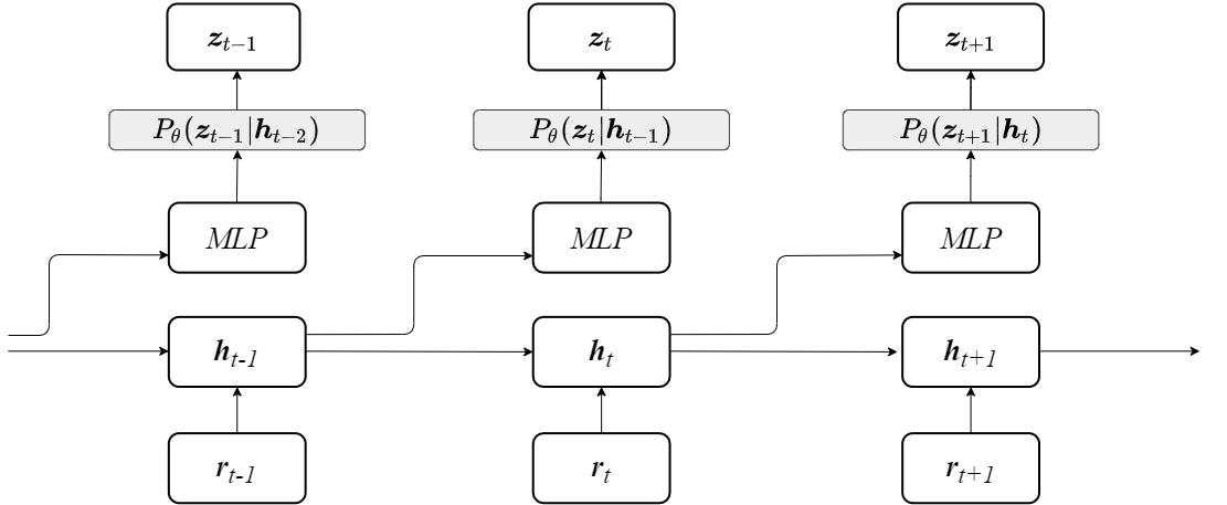
Figure 1: Generative model of VHVM. The generative MLP takes as input $\{\boldsymbol{r}_{1:t-1}\}$ and predicts the next-period latent factor $\boldsymbol{z}_{t}$, conditioned on which we can obtain an estimate of the covariance matrix $\boldsymbol{\Sigma}_{t}$.

3.3 Inference Model

The inference model defines the joint distribution $q_{\phi}(\boldsymbol{L}_{1:T},\boldsymbol{z}_{1:T}|\boldsymbol{r}_{1:T})$ which we factorise as follows:

$$q_{\phi}(\boldsymbol{L}_{1:T},\boldsymbol{z}_{1:T}|\boldsymbol{r}_{1:T})=\prod_{t=1}^{T}q_{\phi}(\boldsymbol{L}_{t}|\boldsymbol{z}_{t})q_{\phi}(\boldsymbol{z}_{t}|\boldsymbol{r}_{1:t}),$$ (15)

where the posterior distribution over latent variable $q_{\phi}(\boldsymbol{z}_{t}|\boldsymbol{r}_{1:t})$ is parameterised by the encoder (MLP) of the VAE:

$$\{\boldsymbol{\mu}_{z,t},\boldsymbol{\Sigma}_{z,t}\}_{post}=MLP_{Inf}(\boldsymbol{h}_{t});$$ (16)

this represents the filtering distribution, which is our inference of $\boldsymbol{z}_{t}$ given the most up-to-date observational data $\boldsymbol{r}_{1:t}$. Since $q_{\phi}(\boldsymbol{z}_{t}|\boldsymbol{r}_{1:t})$ is our variational approximation of the actual posterior $P_{\theta}(\boldsymbol{z}_{t}|\boldsymbol{r}_{1:t})$, we see from (8) that maximising the $ELBO(\theta,\phi)$ w.r.t. $\phi$ is equivalent to minimising the KL divergence between the variational posterior and the actual posterior. The deterministic function to obtain $\boldsymbol{L}_{t}$ given $\boldsymbol{z}_{t}$ is the same as in the generative model: i.e. $q_{\phi}(\boldsymbol{L}_{t}|\boldsymbol{z}_{t})=P_{\theta}(\boldsymbol{L}_{t}|\boldsymbol{z}_{t})$, since this simply torch.tril_indices() followed by Softplus.

To summarise, VHVM is consisted of three neural networks: (1) an MLP ($MLP_{Gen}$) for the prior prediction model $P_{\theta}(\boldsymbol{z}_{t}|\boldsymbol{r}_{1:t-1})$, also known as the decoder of the VAE which models the transition of the latent variable; (2) an MLP ($MLP_{Inf}$) for the variational posterior $q_{\phi}(\boldsymbol{z}_{t}|\boldsymbol{r}_{1:t})$, which is the encoder the VAE; (3) a GRU with hidden states $\boldsymbol{h}_{t}$ to carry sequential information about the multivariate returns process {$\boldsymbol{r}_{1:T}$} and is shared by the generative and inference models.

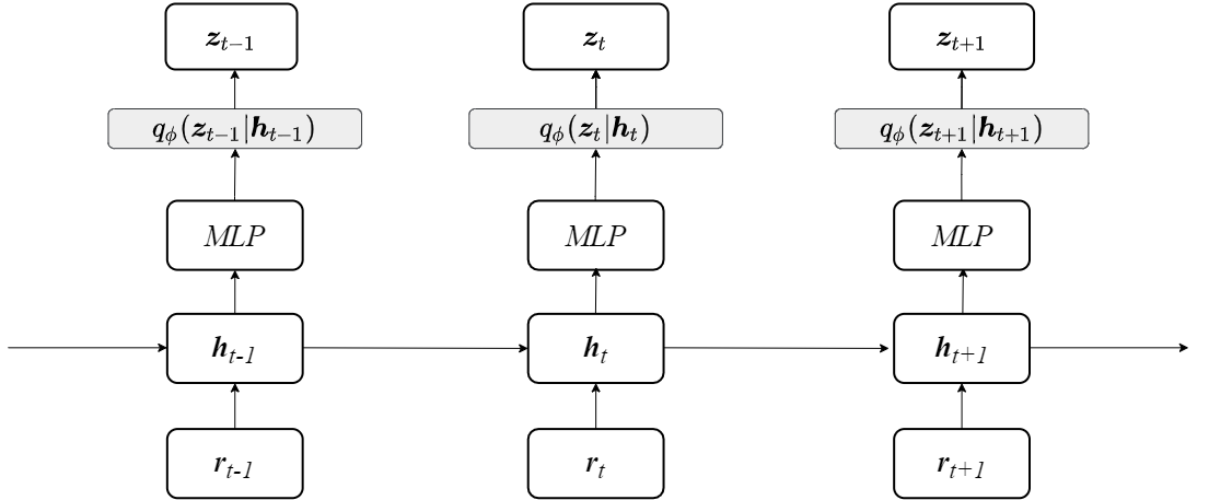
Figure 2: Inference model of VHVM. The Inference MLP takes as input $\{\boldsymbol{r}_{1:t}\}$ and paratermises the filter distribution over $\boldsymbol{z}_{t}$, conditioned on which we can obtain the posterior estimate of the covariance matrix $\boldsymbol{\Sigma}_{t}$.

3.4 Model Training and Prediction

To perform variational inference we seek to maximise the $ELBO(\theta,\phi)$ w.r.t. $\theta$ and $\phi$ jointly (Kingma and Welling, 2014). The expression for the evidence lower bound is given in (17). VHVM is designed to output one step-ahead volatility prediction. When new observations become available, we update the hidden state $\boldsymbol{h}_{t}$ of the GRU, which serves as the input to the prediction network $MLP_{Gen}$ to predict the next period lower Cholesky matrix.

$$ELBO(\theta,\phi)=\sum_{n=1}^{T}\mathbb{E}_{\boldsymbol{z}_{t}\sim q_{\phi}}[logP_{\theta}(\boldsymbol{r}_{t}|\boldsymbol{z}_{t})]-KL(q_{\phi}(\boldsymbol{z}_{t}|\boldsymbol{r}_{1:t})||P_{\theta}(\boldsymbol{z}_{t}|\boldsymbol{r}_{1:t-1})),$$ (17)

4 Experiments

We test VHVM on foreign exchange data obtained from the Trading Academy website (eatradingacademy.com). We compute daily log returns using data from the period 24/01/2012 to 23/01/2022 (a total of 3653 observations), from which we remove weekend readings where the change in asset price was 0. We constructed various portfolios using our collection of FX series for $n=$ 5, 10, 20, and 50. For model construction, we used a train:validation:test ratio of 80:10:10 and training for 50 epoches.

For model benchmarking, we compared VHVM against three benchmarks: (1) the DCC-GARCH model (Engle, 2002), (2) a factor SV model with MCMC sampling (Hosszejni and Kastner, 2021), and (3) Neural Stochastic Volatility model (Luo et al., 2018). The three baselines are representative models from the current approaches to volatility forecasting: GARCH models, SV models, and deep learning based models. We have chosen DCC-GARCH due to its ability to model dynamic conditional correlation between assets; we implemented the model in R using the package ”rmgarch” (Galanos, 2022). For the factor SV model with MCMC sampler (MCMC-SV), we used the recently developed ”factorstochvol” package in R (Hosszejni and Kastner, 2021).

The Neural Stochastic Volatility model (NSVM) Luo et al. (2018) is perhaps most relevant to our work since it was also designed under the VRNN framework. NSVM uses four recurrent neural networks to model temporal dynamics: one for the observed returns series $\boldsymbol{r}_{t}$ and another for the latent factor $\boldsymbol{z}_{t}$ in the generative model; similarly for the inference model. In our model however, we attempted to keep the number of model parameters low by using only one RNN but inputting the hidden state at different time steps to perform prediction and inference. Another key difference between NSVM and VHVM is that the output of NSVM is a low-rank approximation of the time-varying covariance matrix, whereas VHVM outputs the full covariance matrix. A low rank approximation may offer faster computations for higher dimensional portfolios, however we show that VHVM is consistently better in terms of performance.

For model evaluation, we perform one step-ahead covariance matrix forecasting on the test set, and following Wu et al. (2013) and Luo et al. (2018) use the log likelihood (2) as our performance metric since it describes the likelihood of the observed data falling under our estimated distribution. We have also included the hyperparameters of our model and the baselines in the Appendix for reproduction purposes.

5 Results and Discussion

In Table 1 to 5 we show the performance of VHVM against the three baseline models: NSVM, DCC-GARCH, and MCMC-SV on various 5 dimensional FX portfolios. For every time step we forecast a $5\times 5$ covariance matrix and in the tables we report the cumulative log likelihood of the test set. We have highlighted in bold the best performing model in terms of log likelihood (higher is better). We observe that VHVM performs best in 17 out of the 20 constructed portfolios. The neural network baseline NSVM however performs best in only one of the portfolios. As previously mentioned, the two key difference between VHVM and NSVM are: (1) VHVM uses a single RNN to carry information about $\boldsymbol{r}_{1:t}$ and the hidden state at different time steps is used for forecasting ($\boldsymbol{h}_{t-1}$)/inference ($\boldsymbol{h}_{t}$), whereas NSVM uses four separate RNNs to model $\boldsymbol{z}_{t}$ and $\boldsymbol{r}_{t}$ in generation and inference; (2) NSVM outputs low rank approximations of the covariance matrix whereas VHVM outputs estimates of the full covariance matrix. We believe the simpler structure (fewer parameters) of our model has helped to reduce overfitting, and parameterising the full covariance matrix is more expressive than a low rank approximation at the expense of computational complexity ($O(n^{2})$ vs $O(n)$)

Table 1: Log likelihoods of 5 dimensional Euro-denominated portfolios. The best performing model is highlighted in bold; higher log likelihood is better.

FX pairs	VHVM (ours)	NSVM	DCC-GARCH	MCMC-SV
EURAUD, EURHKD, EURCAD, EURCNY, EURDKK	$\boldsymbol{-1013.489}$	-1362.564	-1134.183	-1144.132
EURCNY, EURGBP, EURHKD, EURHUF, EURIDR	$\boldsymbol{-1189.944}$	-1456.841	-1235.496	-1279.841
EURGBP, EURJPY, EURKRW, EURMXN, EURNOK	$\boldsymbol{-1418.791}$	-1493.457	-1506.990	-1471.722
EURJPY, EURNZD, EURRUB, EURSGD, EURTHUB	$\boldsymbol{-1222.507}$	-1331.243	-1301.942	-1262.875

Table 2: Log likelihoods of 5 dimensional GBP-denominated portfolios. The best performing model is highlighted in bold; higher log likelihood is better.

FX pairs	VHVM	NSVM	DCC-GARCH	MCMC-SV
GBPAUD, GBPBGN, GBPBRL, GBPCAD, GBPCHF	$\boldsymbol{-1156.903}$	-1564.931	-1328.515	-1300.182
GBPCHF, GBPCNY, GBPDKK, GBPHKD, GBPILS	$\boldsymbol{-898.588}$	-1571.065	-1047.304	-1076.312
GBPCNY, GBPINR, GBPJPY, GBPMXN, GBPKRW	$\boldsymbol{-1142.915}$	-1400.454	-1248.320	-1211.203
GBPRUB, GBPSEK, GBPTRY, GBPJPY, GBPCAD	-1639.355	$\boldsymbol{-1628.892}$	-2969.575	-2900.870

Table 3: Log likelihoods of 5 dimensional USD-denominated portfolios. The best performing model is highlighted in bold; higher log likelihood is better.

FX pairs	VHVM	NSVM	DCC-GARCH	MCMC-SV
USDAUD, USDBGN, USDCAD, USDCHF, USDCNY	$\boldsymbol{-1309.623}$	-1663.140	-1491.194	-1333.658
USDCNY, USDEUR, USDGBP, USDHKD, USDNZD	-1416.474	-1621.547	-1536.093	$\boldsymbol{-1414.045}$
USDEUR, USDHUF, USDINR, USDJPY, USDNZD	$\boldsymbol{-1237.078}$	-1461.547	-1306.365	-1293.873
USDGBP, USDJPY, USDKRW, USDMXN, USDTRY	$\boldsymbol{-1609.177}$	1807.927	-3490.222	-3129.284

To better gauge the relative performances of the four models, we follow Ismail Fawaz et al. (2019) and plot a critical difference (CD) diagram showing the average ranking of the four model in Figure 3. Within a CD diagram, two models without a statistically significant difference (s.s.d.) in average ranking are connected with a horizontal line; the absence of such lines in Figure 3 indicates that the four models are s.s.d. in performance across the 20 5 dimensional experiments. According to Figure 3 VHVM has the best overall average ranking (1.25), followed by MCMC-SV(2.2), DCC-GARCH(3), and NSVM(3.55). The fact that MCMC-SV performs slightly better than DCC-GARCH is in accordance with claims that SV models are more flexible at modelling heteroscedastic behaviour in financial time series (Shapovalova, 2021).

Table 4: Log likelihoods of 5 dimensional CNY-denominated portfolios. The best performing model is highlighted in bold; higher log likelihood is better.

FX pairs	VHVM	NSVM	DCC-GARCH	MCMC-SV
CNYCAD, CNYEUR, CNYGBP, CNYIDR, CNYJPY	$\boldsymbol{-1171.234}$	-1447.516	-1304.421	-1272.866
CNYKRW, CNYMXN, CNYMYR, CNYRUB, CNYSEK	$\boldsymbol{-1270.803}$	-1346.751	-1384.705	-1335.663
CNYGBP, CNYJPY, CNYSEK, CNYSGD, CNYTHB	$\boldsymbol{-1236.308}$	-1427.729	-1307.665	-1283.031
CNYEUR, CNYMXN, CNYCAD, CNYUSD, CNYTHB	-1604.544	-1592.762	$\boldsymbol{-1535.586}$	-1541.026

Table 5: Log likelihoods of 5 dimensional mixed currency portfolios. The best performing model is highlighted in bold; higher log likelihood is better.

FX pairs	VHVM	NSVM	DCC-GARCH	MCMC-SV
EURAUD, GBPCAD, USDCHF, USDCNY, CNYGBP	$\boldsymbol{-1354.807}$	-1580.274	–1425.861	-1363.748
EURHKD, GBPJPY, USDCHF, CNYRUB, CNYCAD	$\boldsymbol{-1139.711}$	-1331.203	-1290.668	-1271.675
USDGBP, USDJPY, GBPCHF, CNYSGD, GBPMXN	$\boldsymbol{-1312.835}$	-1379.446	-1379.766	-1313.195
CNYEUR, CNYGBP, EURKRW, USDINR, GBPRUB	$\boldsymbol{-1041.155}$	-1247.187	-1172.433	-1146.655

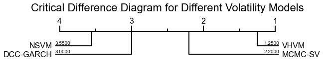
Figure 3: Critical difference diagram showing the comparison between VHVM, NSVM, DCC-GARCH, and MCMC-SV in 5 dimensional FX portfolios.

In Table 6 we show the experimental results for larger portfolios (10, 20, and 50 dimensions). In these experiments we only compare VHVM and NSVM since both DCC-GARCH and MCMC-SV have difficulties scaling up to higher dimensions. The list of currencies included in each portfolio is included in the Appendix. We observe that VHVM performs better than NSVM across all higher dimensional portfolios, consistent with what we observe in the 5 dimensional experiments.

Table 6: Log likelihoods of higher dimensional currency portfolios. The best performing model is highlighted in bold; higher log likelihood is better.

FX pairs	VHVM (ours)	NSVM
$10D_{1}$	$\boldsymbol{-1302.786}$	-3038.413
$10D_{2}$	$\boldsymbol{-1804.729}$	-3117.547
$10D_{3}$	$\boldsymbol{-1472.019}$	-3114.550
$10D_{4}$	$\boldsymbol{-2831.592}$	-3174.692
$20D_{1}$	$\boldsymbol{789.993}$	-6061.243
$20D_{2}$	$\boldsymbol{-1334.264}$	-6312.093
$50D$	$\boldsymbol{-2073.592}$	-15180.516

6 Conclusion

In this paper we propose Variational Heteroscedastic Volatility model (VHVM): an end-to-end neural network architecture capable of forecasting one step-ahead covariance matrices. VHVM outputs the lower Cholesky decomposition of a time-varying conditional precision matrix, which enforces two necessary constraints of a covariance matrix: symmetry and postive definiteness. Furthermore, by setting the neural network to output the precision matrix, we bypass the computationally expensive matrix conversion step in the evaluation of the multivariate normal log likelihood function. We demonstrated the effectiveness of VHVM against GARCH, SV, and deep learning baseline models and we observed that VHVM consistently outperformed its competitors.

References

- Aguilar and West (2000) Aguilar, O. and West, M., Bayesian dynamic factor models and portfolio allocation. Journal of Business and Economic Statistics, 2000, 18, 338–357.
- Aydemir (1998) Aydemir, A., Volatility Modelling in Finance, 1998 (Butterworth-Heinemann: Oxford).
- Bandara et al. (2019) Bandara, K., Shi, P., Bergmeir, C., Hewamalage, H., Tran, Q. and Seaman, B., Sales Demand Forecast in E-commerce Using a Long Short-Term Memory Neural Network Methodology. In Proceedings of the Neural Information Processing, edited by T. Gedeon, K.W. Wong and M. Lee, pp. 462–474, 2019 (Springer International Publishing: Cham).
- Bauwens et al. (2006) Bauwens, L., Laurent, S. and Rombouts, J.V., Multivariate GARCH models: A survey. Journal of Applied Econometrics, 2006, 21, 79–109.
- Bayer and Osendorfer (2014) Bayer, J. and Osendorfer, C., Learning Stochastic Recurrent Networks. arXiv preprint, 2014, pp. 1–9.
- Blei et al. (2017) Blei, D.M., Kucukelbir, A. and McAuliffe, J.D., Variational Inference: A Review for Statisticians. Journal of the American Statistical Association, 2017, 112, 859–877.
- Bollerslev (1986) Bollerslev, T., Generalised Autoregressive Conditional Heteroskedasticity. Journal of Econometrics, 1986, 31, 307–327.
- Bollerslev et al. (1988) Bollerslev, T., Engle, R.F. and Wooldridge, J.M., A Capital Asset Pricing Model with Time-Varying Covariances. Journal of Political Economy, 1988, 96, 116–131.
- Böse et al. (2017) Böse, J.H., Flunkert, V., Gasthaus, J., Januschowski, T., Lange, D., Salinas, D., Schelter, S., Seeger, M. and Wang, Y., Probabilistic Demand Forecasting at Scale. Proc. VLDB Endow., 2017, 10, 1694–1705.
- Chan and Grant (2016) Chan, J.C. and Grant, A.L., Modeling energy price dynamics: GARCH versus stochastic volatility. Energy Economics, 2016, 54, 182–189.
- Cho et al. (2014) Cho, K., van Merrienboer, B., Bahdanau, D. and Bengio, Y., On the Properties of Neural Machine Translation: Encoder–Decoder Approaches. In Proceedings of the In Eighth Workshop on Syntax, Semantics and Structure in Statistical Translation (SSST-8), 2014.
- Christodoulakis and Satchell (2002) Christodoulakis, G.A. and Satchell, S.E., Correlated ARCH (CorrARCH): Modelling the time-varying conditional correlation between financial asset returns. European Journal of Operational Research, 2002, 139, 351–370.
- Christoffersen and Diebold (2000) Christoffersen, P.F. and Diebold, F.X., How Relevant is Volatility Forecasting for Financial Risk Management ?. The Review of Economics and Statistics, 2000, 82, 12–22.
- Chu et al. (2017) Chu, J., Chan, S., Nadarajah, S. and Osterrieder, J., GARCH Modelling of Cryptocurrencies. Journal of Risk and Financial Management, 2017, 10, 17.
- Chung et al. (2015) Chung, J., Kastner, K., Dinh, L., Goel, K., Courville, A. and Bengio, Y., A recurrent latent variable model for sequential data. In Proceedings of the Advances in Neural Information Processing Systems, Vol. 2015-January, pp. 2980–2988, 2015.
- Denton and Fergus (2018) Denton, E. and Fergus, R., Stochastic Video Generation with a Learned Prior. In Proceedings of the 35th International Conference on Machine Learning, ICML 2018, Vol. 3, pp. 1906–1919, 2018.
- Diebold and Nerlove (1989) Diebold, F.X. and Nerlove, M., The dynamics of exchange rate volatility: A multivariate latent factor ARCH model. Journal of Applied Econometrics, 1989, 4, 1–21.
- Dorta et al. (2018) Dorta, G., Vicente, S., Agapito, L., Campbell, N.D. and Simpson, I., Structured Uncertainty Prediction Networks. Proceedings of the IEEE Computer Society Conference on Computer Vision and Pattern Recognition, 2018, pp. 5477–5485.
- Du et al. (2011) Du, X., Yu, C.L. and Hayes, D.J., Speculation and volatility spillover in the crude oil and agricultural commodity markets: A Bayesian analysis. Energy Economics, 2011, 33, 497–503.
- Engle (1982) Engle, R., Autoregressive Conditional Heteroscedasticity with Estimates of the Variance of United Kingdom Inflation. Econometrica, 1982, 50, 987–1007.
- Engle (2002) Engle, R., Dynamic Conditional Correlation. Journal of Business and Economic Statistics, 2002, 20, 339–350.
- Engle and Kroner (1995) Engle, R. and Kroner, K., Multivariate Simultaneous Generalized Arch. Econometric Theory, 1995, 11, 122–150.
- Engle and Patton (2007) Engle, R.F. and Patton, A.J., What good is a volatility model?. Forecasting Volatility in the Financial Markets, 2007, 1, 47–63.
- Escobar-Anel et al. (2022) Escobar-Anel, M., Gollart, M. and Zagst, R., Closed-form portfolio optimization under GARCH models. Operations Research Perspectives, 2022, 9, 100216.
- Fabius and van Amersfoort (2015) Fabius, O. and van Amersfoort, J.R., Variational recurrent auto-encoders. 3rd International Conference on Learning Representations, ICLR 2015 - Workshop Track Proceedings, 2015, pp. 1–5.
- Fama (1965) Fama, E.F.., The Behavior of Stock-Market Prices Author ( s ): Eugene F . Fama Published by : The University of Chicago Press Stable. The Journal of Business, 1965, 38, 34–105.
- Fraccaro et al. (2016) Fraccaro, M., Sønderby, S.K., Paquet, U. and Winther, O., Sequential neural models with stochastic layers. In Proceedings of the Advances in Neural Information Processing Systems, pp. 2207–2215, 2016.
- Franceschi et al. (2020) Franceschi, J.Y., Delasalles, E., Chen, M., Lamprier, S. and Gallinari, P., Stochastic latent residual video prediction. In Proceedings of the 37th International Conference on Machine Learning, ICML 2020, Vol. PartF16814, pp. 3191–3204, 2020.
- Galanos (2022) Galanos, A., Chapter title. rmgarch: Multivariate GARCH models. R package version 1.3-9., 2022.
- Galanos and Kley (2022) Galanos, A. and Kley, T., Chapter title. rugarch: Univariate GARCH Models R package version 1.4-7, 2022.
- Glosten et al. (1993) Glosten, L.R., Jagannathan, R. and Runkle, D.E., On the Relation between the Expected Value and the Volatility of the Nominal Excess Return on Stocks. The Journal of Finance, 1993, 48, 1779–1801.
- Hansen and Lunde (2005) Hansen, P.R. and Lunde, A., A forecast comparison of volatility models: Does anything beat a GARCH(1,1)?. Journal of Applied Econometrics, 2005, 20, 873–889.
- Hassan and Malik (2007) Hassan, S.A. and Malik, F., Multivariate GARCH modeling of sector volatility transmission. Quarterly Review of Economics and Finance, 2007, 47, 470–480.
- Hosszejni and Kastner (2021) Hosszejni, D. and Kastner, G., Modeling Univariate and Multivariate Stochastic Volatility in R with stochvol and factorstochvol. Journal of Statistical Software, 2021, 100, 1–34.
- Huang et al. (2010) Huang, Y., Su, W. and Li, X., Comparison of BEKK GARCH and DCC GARCH Models: An Empirical Study. In Proceedings of the Advanced Data Mining and Applications, edited by L. Cao, J. Zhong and Y. Feng, pp. 99–110, 2010 (Springer Berlin Heidelberg: Berlin, Heidelberg).
- Ismail Fawaz et al. (2019) Ismail Fawaz, H., Forestier, G., Weber, J., Idoumghar, L. and Muller, P.A., Deep learning for time series classification: a review. Data Mining and Knowledge Discovery, 2019, 33, 917–963.
- Jacouier et al. (1994) Jacouier, E., Polson, N.G. and Rossl, P.E., Bayesian analysis of stochastic volatility models. Journal of Business and Economic Statistics, 1994, 12, 371–389.
- J.Duan (1995) J.Duan, The GARCH option pricing model. Mathematical Finance, 1995, 5, 13–32.
- Jebran et al. (2017) Jebran, K., Chen, S., Ullah, I. and Mirza, S.S., Does volatility spillover among stock markets varies from normal to turbulent periods? Evidence from emerging markets of Asia. Journal of Finance and Data Science, 2017, 3, 20–30.
- Karl et al. (2017) Karl, M., Soelch, M., Bayer, J. and Van Der Smagt, P., Deep variational Bayes filters: Unsupervised learning of state space models from raw data. In Proceedings of the 5th International Conference on Learning Representations, ICLR 2017 - Conference Track Proceedings, ii, pp. 1–13, 2017.
- Kingma and Welling (2014) Kingma, D.P. and Welling, M., Auto-encoding variational bayes. In Proceedings of the 2nd International Conference on Learning Representations, ICLR 2014 - Conference Track Proceedings, pp. 1–14, 2014.
- Krishnan et al. (2017) Krishnan, R.G., Shalit, U. and Sontag, D., Structured inference networks for nonlinear state space models. In Proceedings of the 31st AAAI Conference on Artificial Intelligence, AAAI 2017, pp. 2101–2109, 2017.
- Li et al. (2018) Li, Y., Yu, R., Shahabi, C. and Liu, Y., Diffusion Convolutional Recurrent Neural Network: Data-Driven Traffic Forecasting. In Proceedings of the 6th International Conference on Learning Representations, ICLR 2018, Vancouver, BC, Canada, April 30 - May 3, 2018, Conference Track Proceedings, 2018, OpenReview.net.
- Long et al. (2020) Long, H.V., Jebreen, H.B., Dassios, I. and Baleanu, D., On the statistical garch model for managing the risk by employing a fat-tailed distribution in finance. Symmetry, 2020, 12, 1–15.
- Luo et al. (2018) Luo, R., Zhang, W., Xu, X. and Wang, J., A neural stochastic volatility model. In Proceedings of the 32nd AAAI Conference on Artificial Intelligence, AAAI 2018, pp. 6401–6408, 2018.
- Malik (2005) Malik, A.K., European exchange rate volatility dynamics: An empirical investigation. Journal of Empirical Finance, 2005, 12, 187–215.
- Nelson (1991) Nelson, D., Conditional Heteroskedasticity in Asset Returns : A New Approach. Econometrica, 1991, 59, 347–370.
- Pitt and Shephard (1999) Pitt, M.K. and Shephard, N.In Time varying covariances: a factor stochastic volatility approach, pp. 547–570 ((edited by j.m. bernardo, j.o. berger, a.p. dawid and a.f.m smith) edn), 1999 (Oxford University Press: Oxford).
- Platanioti et al. (2005) Platanioti, K., McCoy, E. and Stephens, D., A Review of Stochastic Volatility: Univariate and Multivariate Models [online]. London: , 2005. (accessed ????).
- Poon and Granger (2003) Poon, S.H. and Granger, C.W.J., Forecasting Volatility in Financial Markets : A Review. Journal of Economic Literature, 2003, 41, 478–539.
- Ranković et al. (2016) Ranković, V., Drenovak, M., Urosevic, B. and Jelic, R., Mean-univariate GARCH VaR portfolio optimization: Actual portfolio approach. Computers and Operations Research, 2016, 72, 83–92.
- Schwert (1989) Schwert, G., Why does stock market volatility change with time?. The Journal of Finance, 1989, 44, 1115–1153.
- Shapovalova (2021) Shapovalova, Y., Exact and approximate methods for bayesian inference: stochastic volatility case study. Entropy, 2021, 23.
- Sheppard et al. (2022) Sheppard, K., Khrapov, S., Lipták, G., mikedeltalima, Capellini, R., alejandro cermeno, Hugle, esvhd, bot, S., Fortin, A., JPN, Judell, M., Li, W., Adams, A., jbrockmendel, Rabba, M., Rose, M.E., Tretyak, N., Rochette, T., Leo, U., RENE-CORAIL, X., Du, X. and syncoding, bashtage/arch: Release 5.2.0. , 2022.
- Tse and Tsui (2002) Tse, Y.K. and Tsui, A.K., A multivariate generalized autoregressive conditional heteroscedasticity model with time-varying correlations. Journal of Business and Economic Statistics, 2002, 20, 351–362.
- Van Der Weide (2002) Van Der Weide, R., GO-GARCH: A multivariate generalized orthogonal GARCH model. Journal of Applied Econometrics, 2002, 17, 549–564.
- Wu et al. (2013) Wu, Y., Lobato, J.M.H. and Ghahramani, Z., Dynamic covariance models for multivariate financial time series. In Proceedings of the 30th International Conference on Machine Learning, ICML 2013, Vol. 28, pp. 1595–1603, 2013.
- Wuertz et al. (2017) Wuertz, D., Setz, T., Chalabi, Y., Boudt, C., Chausse, P. and Miklovac, M., Chapter title. fGarch: Autoregressive Conditional Heteroskedastic Modelling R package version 3042.83.2, 2017.
- Yin and Barucca (2022) Yin, Z. and Barucca, P., Neural Generalised AutoRegressive Conditional Heteroskedasticity. arXiv preprint, 2022, pp. 1–13.