Hypercomplex Neural Architectures
for Multi-View Breast Cancer Classification

Abstract

Traditionally, deep learning methods for breast cancer classification perform a single-view analysis. However, radiologists simultaneously analyze all four views that compose a mammography exam, owing to the correlations contained in mammography views, which present crucial information for identifying tumors. In light of this, some studies have started to propose multi-view methods. Nevertheless, in such existing architectures, mammogram views are processed as independent images by separate convolutional branches, thus losing correlations among them. To overcome such limitations, in this paper we propose a novel approach for multi-view breast cancer classification based on parameterized hypercomplex neural networks. Thanks to hypercomplex algebra properties, our networks are able to model, and thus leverage, existing correlations between the different views that comprise a mammogram, thus mimicking the reading process performed by clinicians. The proposed methods are able to handle the information of a patient altogether without breaking the multi-view nature of the exam. We define architectures designed to process two-view exams, namely PHResNets, and four-view exams, i.e., PHYSEnet and PHYBOnet. Through an extensive experimental evaluation conducted with publicly available datasets, we demonstrate that our proposed models clearly outperform real-valued counterparts and also state-of-the-art methods, proving that breast cancer classification benefits from the proposed multi-view architectures. We also assess the method’s robustness beyond mammogram analysis by considering different benchmarks, as well as a finer-scaled task such as segmentation. Full code and pretrained models for complete reproducibility of our experiments are freely available at https://github.com/ispamm/PHBreast.

I Introduction

Among the different types of cancer that affect women worldwide, breast cancer alone accounts for almost one-third, making it by far the cancer with highest incidence among women [1]. For this reason, early detection of this disease is of extreme importance and, to this end, screening mammography is performed annually on all women above a certain age [2, 3]. During a mammography exam, two views of the breast are taken, thus capturing it from above, i.e., the craniocaudal (CC) view, and from the side, i.e., the mediolateral oblique (MLO) view. More in detail, the CC and MLO views of the same breast are known as ipsilateral views, while the same view of both breasts as bilateral views. Importantly, when reading a mammogram, radiologists examine the views by performing a double comparison, that is comparing ipsilateral views along with bilateral views, as each comparison provides valuable information. Such multi-view analysis has been found to be essential in order to make an accurate diagnosis of breast cancer [4, 5].

Recently, many works are employing deep learning (DL)-based methods in the medical field and, especially, for breast cancer classification and detection with encouraging results [6, 7, 8, 9, 10, 11, 12, 13, 14, 15, 16, 17]. Inspired by the multi-view analysis performed by radiologists, several recent studies try to adopt a multi-view architecture in order to obtain a more robust and performing model [18, 19, 20, 21, 22, 23, 24, 25, 26, 27, 28, 29].

Such approaches often implement multi-view frameworks based on multi-path architectures. However, there are several issues associated with such a method in the context of multi-view learning. As a matter of fact, a recent study demonstrates that a simple multi-path network can suffer from several problems [19]. To begin with, it is observed that the model can favor one of the two views during learning, thus relying mostly on that single view and not truly taking advantage of the multi-view input. Additionally, the model might fail entirely in leveraging the correlated views and actually worsen the performance with respect to its single-view counterpart [19, 30]. Thus, it is made clear that improving the ability of deep networks to truly exploit the information contained in multiple views is still a largely open research question. To address and overcome these problems, we leverage a novel technique in deep learning, which relies in exotic algebraic systems, such as quaternions and, more in general, hypercomplex ones.

In recent years, quaternion neural networks (QNNs) have gained a lot of interest in a variety of applications [31, 32, 33, 34, 35, 36]. The reason for this is the particular properties that characterize these models. As point of fact, thanks to the quaternion algebra rules on which these models are based (e.g., the Hamilton product), quaternion networks possess the capability of modeling interactions between input channels, thus capturing internal latent relations within them and additionally reducing the total number of parameters by $75\%$, while still attaining comparable performance to its real-valued counterparts. Furthermore, built upon the idea of QNNs, the recent parameterized hypercomplex neural networks (PHNNs) generalize hypercomplex multiplications as a sum of Kronecker products, going beyond quaternion algebra, thus improving previous shortcomings by making these models applicable to any $n$-dimensional input (instead of just $3$D/$4$D as the quaternion domain) thanks to the introduction of the parameterized hypercomplex multiplication (PHM) and convolutional (PHC) layer [37, 38].

Motivated by the problems mentioned above and the benefits of hypercomplex models, we propose a novel framework of multi-view learning for breast cancer classification based on PHNNs, taking a completely different approach with respect to existing methods in the literature. More in detail, we propose a family of parameterized hypercomplex ResNets (PHResNets) able to process ipsilateral views corresponding to one breast, i.e., two views. We also design two parameterized hypercomplex networks for four views, namely PHYBOnet and PHYSEnet, involving respectively a Bottleneck with $n=4$, to process learned features in a joint fashion, performing a patient-level analysis, and a Shared Encoder with $n=2$, to learn stronger representations of the ipsilateral views by sharing the weights between bilateral views, focusing on a breast-level analysis.

The advantages of our approach are manifold. Firstly, instead of handling the mammographic views independently, which results in losing significant correlations, our models process them as a unique component, without breaking the original nature of the exam. Secondly, thanks to hypercomplex algebra properties, the proposed models are endowed with the capability of preserving existing latent relations between views by modeling and capturing their interactions, thus mimicking the examination process of radiologists in real-life settings. Thirdly, our parameterized hypercomplex networks are characterized by the number of free parameters halved, when $n=2$, and reduced by $1/4$, when $n=4$, with respect to their real-valued counterparts. Finally, the proposed approach is portable and flexible, being PHC layers easily integrable in any neural network and capable of processing an arbitrary number of views, thus easily applicable for other types of multi-view or multimodal problems.

We evaluate the effectiveness of our approach on two publicly available benchmark datasets of mammography images, namely CBIS-DDSM [39] and INbreast [2]. We conduct a meticulous experimental evaluation that demonstrates how our proposed models, owing to the aforementioned abilities, possess the means for properly leveraging information contained in multiple mammographic views and thus far exceed the performance of both real-valued baselines and state-of-the-art methods. Finally, we further validate the proposed method on two additional benchmark datasets, i.e., Chexpert [40] for chest X-rays and BraTS19 [41, 42] for brain MRI, to prove the generalizability of the proposed approach in different applications and medical exams, going beyond mammograms and classification.

More concretely, our contributions are:

1. We present a novel approach for multi-view breast cancer classification, which processes mammographic views as a single exam, gaining advantages from the different views to output the diagnosis, as radiologists actually do.

2. We introduce two multi-level models, namely PHYBOnet and PHYSEnet, for the four-view scenario, that involve two steps focusing on a breast-level analysis first and on a patient-level analysis then and vice versa, in order to unveil the best way to process four-view exams.

3. We evaluate the validity of our assumptions on two publicly available benchmarks of mammography exams, performing experiments with two and with four-view exams, with our parameterized hypercomplex models far exceeding state-of-the-art methods.

4. We show the robustness and flexibility of the proposed framework by considering different medical exams and tasks, that is, multi-view multi-label chest X-ray classification, overall survival prediction from multimodal brain MRI scans and multimodal brain tumor segmentation.

The rest of the paper is organized as follows. Section II gives a detailed overview of the multi-view approach for breast cancer analysis, delving into why it is important to design a painstaking multi-view method, Section III provides theoretical aspects and concepts of hypercomplex models, and Section IV presents the proposed method. The experiments are set up in Section V and evaluated in Section VI. A summary of the proposed models with specific data cases is provided in Section VIII, while conclusions are drawn in Section IX.

II Multi-View Approach in Breast Cancer Analysis

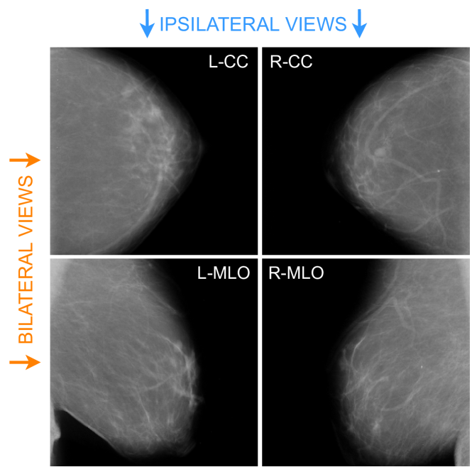
Figure 1: Example of a mammography exam from the CBIS-DDSM dataset with the four views: left CC (L-CC), right CC (R-CC), left MLO (L-MLO) and right MLO (R-MLO). Horizontal couples are bilateral views (orange), while vertical couples are ipsilateral views (blue).

Several types of imaging modalities exist for the detection process of breast cancer, such as mammography, ultrasound, biopsy and so on. Among these, mammography is considered the best imaging method for breast cancer screening and the most effective for early detection [3]. A mammography exam comprises four X-ray images produced by the recording of two views for each breast: the craniocaudal (CC) view, which is a top to bottom view, and a mediolateral oblique (MLO) view, which is a side view. The diagnosis procedure adopted by radiologists consists in looking for specific abnormalities, the most common being: masses, calcifications, architectural distortions of breast tissue, and asymmetries (when comparing the two breasts and the two views) [2]. During the reading of a mammography exam, employing multiple views is crucial in order to make an accurate diagnosis as they retain highly correlated characteristics. Admittedly, comparing ipsilateral views (CC and MLO views of the same breast) helps to detect eventual tumors, as sometimes they are visible only in one of the two views, and additionally helps to analyze the 3D structure of masses. Whereas, studying bilateral views (same view of both breasts) helps in locating masses as asymmetries between them are an indicating factor [5]. An example of a complete mammogram exam with ipsilateral and bilateral views is shown in Fig. 1.

Given the multi-view nature of the exam and the multi-view approach employed by radiologists, many works are focusing on utilizing two or four views for the purpose of classifying breast cancer, with the goal of leveraging the information coming from ipsilateral and/or bilateral views. In point of fact, studies have shown that a model employing multiple views can learn to generalize better compared to its single-view counterpart, increasing its discriminative power, while also reducing the number of false positives and false negatives [9, 6, 18].

On one hand, some works show the advantages of leveraging multiple views by adopting simple approaches, such as a method consisting in just taking the average of the predictions given by the same model when fed the two ipsilateral views [6]. On the other hand, more complex approaches consist in designing a multi-view architecture that should exploit correlations for learning and not just at inference time. Recent techniques for leveraging multiple views from a mammography exam propose architectures comprised of multiple convolutional neural networks (CNN) paths or columns, where each column processes a different view and its output is then concatenated together and fed to a number of fully connected layers to obtain the final output [19, 18, 20, 21, 23, 22, 24, 25]. A recent study proposes an approach to leverage the complete mammography exam, thus comprised of four views. Alternatively, a number of works [20, 26, 21, 22] adopt the same idea of having multiple columns but instead focus on using just two ipsilateral views.

Even though multimodal methods have been employed in a variety of recent deep learning works for breast cancer analysis, not much attention has been paid to how a DL model actually leverages information contained in the multiple views. Indeed, a recent study shows that such multimodal approaches suffer from the fact that the model might actually fail to exploit such information, leading to a counter-intuitive situation in which the single-view counterpart outperforms the multi-view one. Therefore, just employing an architecture with multiple columns for each view is not enough to really leverage the knowledge coming from the correlated inputs [19]. Even in other applications of multimodal learning (e.g., involving speech or text), it is a common phenomenon that DL networks not properly modeled fail to utilize the information contained in the different input modalities [30]. Therefore, when processing multi-view exams, a painstaking and meticulous method has to be developed. To this end, we propose to leverage a novel method based on hypercomplex algebra, whose properties are described in the following section.

III Quaternion and Hypercomplex Neural Networks

Quaternion and hypercomplex neural networks have their foundations in a hypercomplex number system ${\mathbb{H}}$ equipped with its own algebra rules to regulate additions and multiplications. Hypercomplex numbers generalize a plethora of algebraic systems, including complex numbers ${\mathbb{C}}$, quaternions ${\mathbb{Q}}$ and octonions $\mathbb{O}$, among others. A generic hypercomplex number is defined as

$$h=h_{0}+h_{i}{\hat{\imath}}_{i}+\ldots+h_{n}{\hat{\imath}}_{n},\qquad i=1,\ldots,n$$ (1)

whereby $h_{0},\ldots,h_{n}$ are the real-valued coefficients and ${\hat{\imath}}_{i},\ldots,{\hat{\imath}}_{n}$ the imaginary units. The first coefficient $h_{0}$ represents the real component, while the remaining ones compose the imaginary part. Therefore, the algebraic subsets of ${\mathbb{H}}$ are identified by the number of imaginary units and by the algebraic rules that govern the interactions among them. For instance, a complex number has just one imaginary unit, while a quaternion has three imaginary units and the vector product in this domain is not commutative so the Hamilton product has been introduced to multiply two quaternions. Interestingly, a real number can be expressed through eq. (1) by setting $i=0$ and considering the real part only. Being hypercomplex algebras part of the Cayley-Dickson algebras, they always have a dimension equal to a power of $2$, therefore it is important to note that subset domains exist solely at pre-defined dimensions, i.e., $n=2,4,8,16,\ldots$ while no algebra rules have been discovered yet for other values.

The addition operation is performed through an element-wise addition of terms, i.e., $h+p=(h_{0}+p_{0})+(h_{i}+p_{i}){\hat{\imath}}_{i}+\ldots+(h_{n}+p_{n}){\hat{\imath}}_{n}$. Similarly, the scalar product can be formulated with $\alpha h=\alpha h_{0}+\alpha h_{i}{\hat{\imath}}_{i}+\ldots+\alpha h_{n}{\hat{\imath}}_{n}$ by multiplying the scalar to real-valued components. Nevertheless, with the increasing of $n$, Cayley-Dickson algebras lose some properties regarding the vector multiplication, and more specific formulas need to be introduced to model this operation because of imaginary units interplays [43]. Indeed, as an example, quaternions and octonions products are not commutative due to imaginary unit properties for which ${\hat{\imath}}_{1}{\hat{\imath}}_{2}\neq{\hat{\imath}}_{2}{\hat{\imath}}_{1}$. Therefore, quaternion convolutional neural network (QCNN) layers are based on the Hamilton product, which organizes the filter weight matrix to be encapsulated into a quaternion as ${\mathbf{W}}={\mathbf{W}}_{0}+{\mathbf{W}}_{1}{\hat{\imath}}_{1}+{\mathbf{W}}_{2}{\hat{\imath}}_{2}+{\mathbf{W}}_{3}{\hat{\imath}}_{3}$ and to perform convolution with the quaternion input ${\mathbf{x}}={\mathbf{x}}_{0}+{\mathbf{x}}_{1}{\hat{\imath}}_{1}+{\mathbf{x}}_{2}{\hat{\imath}}_{2}+{\mathbf{x}}_{3}{\hat{\imath}}_{3}$ as:

$${\bf{W}}*{\bf{x}}=\left[{\begin{array}[]{*{20}c}\hfill{{\bf{W}}_{0}}&\hfill{-{\bf{W}}_{1}}&\hfill{-{\bf{W}}_{2}}&\hfill{-{\bf{W}}_{3}}\\ \hfill{{\bf{W}}_{1}}&\hfill{{\bf{W}}_{0}}&\hfill{-{\bf{W}}_{3}}&\hfill{{\bf{W}}_{2}}\\ \hfill{{\bf{W}}_{2}}&\hfill{{\bf{W}}_{3}}&\hfill{{\bf{W}}_{0}}&\hfill{-{\bf{W}}_{1}}\\ \hfill{{\bf{W}}_{3}}&\hfill{-{\bf{W}}_{2}}&\hfill{{\bf{W}}_{1}}&\hfill{{\bf{W}}_{0}}\\ \end{array}}\right]*\left[{\begin{array}[]{*{20}c}{{\bf{x}}_{0}\hfill}\\ {{\bf{x}}_{1}\hfill}\\ {{\bf{x}}_{2}\hfill}\\ {{\bf{x}}_{3}\hfill}\\ \end{array}}\right].$$ (2)

Processing multidimensional inputs with QCNNs has several advantages. Indeed, due to the reusing of filter submatrices ${\mathbf{W}}_{i},\;i=0,\ldots,3$ in eq. (2), QCNNs are defined with $1/4$ free parameters with respect to real-valued counterparts with the same architecture structure. Moreover, sharing the filter submatrices among input components allows QCNNs to capture internal relations in input dimensions and to preserve correlations among them [44, 32]. However, this approach is limited to $4$D inputs, thus various knacks are usually employed to apply QCNNs to different $3$D inputs, such as RGB color images. In these cases, a padding channel is concatenated to the three-channel image to build a $4$D image adding, however, useless information. Similarly, when processing grayscale images with QCNNs, the single channel has to be replicated in order to be fed into the quaternion-valued network, without annexing any additional information for the model. Recently, novel approaches proposed to parameterize hypercomplex multiplications and convolutions to maintain QCNNs and hypercomplex algebras advantages, while extending their applicability to any $n$D input [37, 38]. The core idea of these methods is to develop the filter matrix ${\mathbf{W}}$ as a parameterized sum of Kronecker products:

$${\mathbf{W}}=\sum_{i=0}^{n}\mathbf{A}_{i}\otimes\mathbf{F}_{i},$$ (3)

whereby $n$ is a tunable or user-defined hyperparameter that determines the domain in which the model operates (i.e., $n=4$ for the quaternion domain, $n=8$ for octonions, and so on). The matrices $\mathbf{A}_{i}$ encode the algebra rules, that is the filter organization for convolutional layers, while the matrices $\mathbf{F}_{i}$ enclose the weight filters. Both these elements are completely learned from data during training, thus grasping algebra rules or adapting them if no algebra exists for the specific value of $n$ directly from inputs. The parameterized hypercomplex convolutional (PHC) layer is malleable to operate in any $n$D domain by easily setting the hyperparameter $n$, thus extending QCNNs advantages to every multidimensional input. Indeed, parameterized hypercomplex neural networks (PHNNs) can process color images in their natural domain ($n=3$) without adding any uninformative channel (as previously done for QCNNs), while still exploiting hypercomplex algebra properties and preserving correlations and latent relations between channels. Moreover, due to the data-driven fashion in which this approach operates, PHNNs with $n=4$ outperform QCNNs both in terms of prediction accuracy and training as well as inference time [38, 37]. Furthermore, PHC layers employ $1/n$ free parameters with respect to real-valued counterparts, so the user can govern both the domain and the parameters reduction by simply setting the value of $n$.

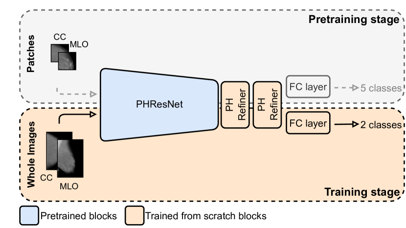
Figure 2: Training pipeline and PHResNet overview. During the pretraining stage the PHResNet is trained on patches with five classes. At training stage on whole images, two PH convolutional refiner blocks are added.

The reason behind the success of this kind of networks is that to detect objects in an image, neural networks have to discover global and local dependencies, where the first ones are related to spatial relations among pixels of the same level (i.e., for an RGB image, the R, G, B channels are different levels), and the second ones implicitly link different levels. In the latter case, implicit local relations for an RGB image are the natural link that exists within the three-channel components defining a pixel. The latter case of correlation among the different levels of the input is usually not taken into account by conventional neural networks that operate in the real domain, as they consider the pixels at different levels as sets of decorrelated points. Considering the multiple dimensions/levels of a sample as unrelated components may break the inner nature of the data, losing information about the inner structure of the sample. Therefore, hypercomplex algebra may be a powerful tool to overcome these limitations as it is able to describe multidimensional data preserving its inner structure by leveraging specific algebra rules. PHNNs can therefore explore both global and local relations, not losing crucial information. Indeed, global relations are modeled as in conventional models (e.g., with convolutional operations), and local relations are instead modeled through the hypercomplex algebra rules. In the mammography scenario, global relations are represented by single-view correlations of objects (e.g., the breast) in the image, while local relations are contained in the multiple views (that is, in the multiple levels) of the whole exam.

Therefore, when input data show some relations at different levels or views, it is possible to equip common convolutional neural networks with PHC layers by easily replacing real-valued operations with hypercomplex ones and choosing the proper domain depending on the input structure, exploiting the advantages of PHNNs.

IV Proposed Method

Figure 3: PHYBOnet architecture. The model first performs a breast-level analysis by taking as input two pairs of ipsilateral views that are handled by two pretrained PH encoder branches with $n=2$. The learned latent representations are then processed in a joint fashion by four PH residual blocks with $n=4$. Finally, the outputs from the two branches are fed to a separate final fully connected layer after a global average pooling operation.

In the following section, we expound the proposed approach and we delineate the structure of our models and the training recipes we adopt. More in detail, we design ad hoc networks for two-view and four-view exams, i.e., a complete mammography exam.

IV-A Multi-view parameterized hypercomplex ResNet

The core idea of our method is to leverage information contained in multiple views through parameterized hypercomplex convolutional (PHC) layers in order to obtain a more performant and robust classifier for breast cancer.

ResNets are among the most widespread models for medical image classification [45, 18, 6, 19, 46, 9, 15]. They are characterized by residual connections that ensure proper gradient propagation during training. A ResNet block is typically defined by:

$$\mathbf{y}=\mathcal{F}(\mathbf{x})+\mathbf{x},$$ (4)

where $\mathcal{F}({\mathbf{x}})$ is usually composed by interleaving convolutional layers, batch normalization (BN) and ReLU activation functions. When equipped with PHC layers, real-valued convolutions are replaced with PHC to build parameterized hypercomplex ResNets (PHResNets), therefore $\mathcal{F}({\mathbf{x}})$ becomes:

$$\mathcal{F}(\mathbf{x})=\text{BN}\left(\text{PHC}\left(\text{ReLU}\left(\text{BN}\left(\text{PHC}\left(\mathbf{x}\right)\right)\right)\right)\right),$$ (5)

in which $\mathbf{x}$ can be any multidimensional input with correlated components. It is worth noting that PH models generalize real-valued counterparts and also monodimensional inputs. As a matter of fact, a PH model with $n=1$ is equivalent to a real-valued model receiving $1$D inputs.

IV-B Parameterized hypercomplex architectures for two views

The proposed multi-view architecture in the case of two views is straightforward: we employ parameterized hypercomplex ResNets (PHResNets) and we fix the hyperparameter $n=2$. The model is depicted in Fig. 2 together with the training strategy we deploy. The two views of the same breast, i.e., ipsilateral views, are fed to the network as a multidimensional input (channel-wise) enabling PHC layers to exploit their correlations. We adopt ipsilateral views instead of bilateral views, as they are two views of the same breast and thus contain information that helps the model in both the detection process and the classification one. Ultimately, the model produces a binary prediction indicating the presence of either a malignant or benign/normal finding (depending on the dataset). In such a manner, the model is able to process the two mammograms as a unique entity and model the interactions between the highly correlated views, mimicking the diagnostic process of radiologists.

IV-C Parameterized hypercomplex architectures for four views

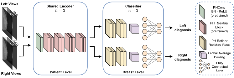
Figure 4: PHYSEnet architecture. The model comprises an initial deep patient-level framework that takes as input two pairs of ipsilateral views which are processed by a pretrained shared PHResNet18 with $n=2$ that serves as encoder. Ultimately, the two learned latent representations are fed to the respective classification branch composed of PH refiner residual blocks with global average pooling and the final fully connected layer to perform the breast-level learning.

IV-C1 Parameterized Hypercomplex Bottleneck network (PHYBOnet)

The first model we propose is shown in Fig. 3, named PH Bottleneck network (PHYBOnet). PHYBOnet is based on an initial breast-level focus and a consequent patient-level one, through the following components: two encoder branches for each breast side with $n=2$, a bottleneck with the hyperparameter $n=4$ and two final classifier layers that produce the binary prediction relative to the corresponding side. Each encoder takes as input two views (CC and MLO) and has the objective of learning a latent representation of the ipsilateral views. The learned latent representations are then merged together and processed by the bottleneck which has $n$ set to $4$ in order for PHC layers to work their magic. Indeed, in this way we additionally obtain a light network since the number of parameters is reduced by $1/4$.

IV-C2 Parameterized Hypercomplex Shared Encoder network (PHYSEnet)

The second architecture we proffer, named Parameterized Hypercomplex Shared Encoder network (PHYSEnet), is depicted in Fig. 4. It has a broader focus on the patient-level analysis through an entire PHResNet18 with $n=2$ as the encoder model, which takes as input two ipsilateral views and whose weights between the two sides (left and right breast) are shared to jointly analyze the whole information of the patient. Then, two final classification branches, consisting of residual blocks and a final fully connected layer, perform a breast-level analysis to output the final prediction for each breast. This design allows the model to leverage information from both ipsilateral and bilateral views. Indeed, thanks to PHC layers, ipsilateral information is leveraged as in the case of two views, while by sharing the encoder between the two sides, the model is also able to take advantage of bilateral information.

IV-D Training procedure

Training a classifier from scratch for this kind of task is very difficult for a number of reasons. For starters, the task itself is much more challenging with respect to the classification of natural images: mammogram images containing benign or malignant tumors present very few differences distinguishable only by trained and skilled clinicians. Additionally, in general, and even more so for such a challenging task, neural models require huge volumes of data for training. However, there are only a handful of publicly available datasets for breast cancer and, on top of that, they are characterized by an extremely limited number of examples. Finally, and most importantly, a lesion occupies only a tremendously small portion of the original image, thus making it arduous to be detected by a model [6], especially if the image is reduced in quality, which is often necessary for memory constraints.

To overcome these challenges, we deploy an ad hoc pretraining strategy divided in two main steps and illustrated in Fig. 2. First, we pretrain the model on patches of mammograms and then we involve the pretrained weights to initialize the network for training on whole images. Indeed, pretraining the network on patches of images that contain either a region of interest (ROI) or a background/normal part of the image, allows the model to learn the features that distinguish malignant from benign tumors [6, 18]. Subsequently, these features are exploited for the training on whole images by initializing the network weights with the patch classifier weights. Such training strategy plays a determining role in boosting the performance of the models as we demonstrate in the experimental Section VI.

V Experimental setup

In this section, we describe the experimental setup of our work that comprises the datasets we consider, the metrics employed for evaluation, model architectures details and training hyperparameters.

V-A Data

We validate the proposed method with two publicly available datasets of mammography images, whose sample summary is presented in Tab. I. We additionally demonstrate the robustness and flexibility of the proposed method on two additional tasks and datasets described herein.

V-A1 CBIS-DDSM

The Curated Breast Imaging Subset of DDSM (CBIS-DDSM) [39] is an updated and standardized version of the Digital Database for Screening Mammography (DDSM). It contains 2478 scanned film mammography images in the standard DICOM format and provides both pixel-level and whole-image labels from biopsy-proven pathology results. Furthermore, for each lesion, the type of abnormality is reported: calcification (753 cases) or mass (891 cases). Importantly, the dataset does not contain healthy cases but only positive ones (i.e., benign or malignant), where for the majority of them a biopsy was requested by the radiologist in order to make a final diagnosis, meaning that the dataset is mainly comprised of the most difficult cases. Additionally, the dataset provides the data divided into splits containing only masses and only calcifications, respectively, in turn split into official training and test sets, characterized by the same level of difficulty. CBIS-DDSM is employed for the training of the patch classifier as well as whole-image classifier in the two-view scenario. It is not used for four-view experiments as the official training/test splits do not contain enough full-exam cases and creating different splits would result in data leakage between patches and whole images. Finally, the images are resized [6] to $600\times 500$ and are augmented with a random rotation between $-25$ and $+25$ degrees and a random horizontal and vertical flip.

V-A2 INbreast

The second dataset employed in this study, INbreast [2], is a database of full-field digital mammography (FFDM) images. It contains 115 mammography exams for a total of 410 images, involving several types of lesions, among which are masses and calcifications. The data splits are not provided, thus they are manually created by splitting the dataset patient-wise in a stratified fashion, using 20% of the data for testing. Finally, INbreast does not provide pathological confirmation of malignancy but BI-RADS labels. Therefore, in the aim of obtaining binary labels, we consider BI-RADS categories 4, 5 and 6 as positive and 1, 2 as negative, whilst ruling out category 3 following the approach of [6]. INbreast is utilized for experiments in both the two-view and four-view scenario and the same preprocessing as CBIS-DDSM is applied.

V-A3 CheXpert

The CheXpert [40] dataset contains 224,316 chest X-rays with both frontal and lateral views and provides labels corresponding to 14 common chest radiographic observations. Images are resized to $320\times 320$ [40] for training and the same augmentation operations as before are applied.

V-A4 BraTS19

BraTS19 [41, 42, 47] is a dataset of multimodal brain MRI scans, providing four modalities for each exam, segmentation maps, demographic information (such as age) and overall survival (OS) data as the number of days for $210$ patients. For training, volumes are resized to $128\times 128\times 128$ and augmented via random scaling between 1 and 1.1 [48] for the task of overall survival prediction. Rather, for segmentation, 2D axial slices are extracted from the volumes and the original shape of $240\times 240$ is maintained.

V-B Evaluation metrics

We adopt AUC (Area Under the ROC Curve) as the main performance metric to evaluate our models, as it is one of the most common metrics employed in medical imaging tasks [19, 18, 6, 20]. The ROC curve summarizes the trade-off between True Positive Rate (TPR) and False Positive Rate (FPR) for a predictive model using different probability thresholds. To further assess network performance, we additionally evaluate our models in terms of classification accuracy. Finally, we employ the Dice score for the segmentation task, which measures the pixel-wise agreement between a predicted mask and its corresponding ground truth.

V-C Training details

We train our models to minimize the binary cross-entropy loss using Adam optimizer [49], with a learning rate of $10^{-5}$ for classification experiments and $2\times 10^{-4}$ for segmentation. Regarding two-view models, the batch size is 8 for PHResNet18, 2 for PHResNet50 and 32 for PHUNet. Instead, for four-view models the batch size is set to 4 and, to overcome the problem of imbalanced data, we utilize a weighted loss assigning a weight to positive examples equal to the number of benign/normal examples divided by the number of positive examples. We adopt two regularization techniques: weight decay at $5\times 10^{-4}$ and early stopping.

TABLE I: Data distribution for splits of CBIS-DDSM and for INbreast when considering two and four views. In the whole table, two views of the same breast are counted as one instance.

CBIS-DDSM
	Mass split				Mass-calc split
	Malignant		Benign		Malignant		Benign/Normal
Train	254		255		480		582
Test	59		83		104		149
INbreast
	Two views				Four views
	Malignant		Benign		Malignant		Benign/Normal
Train	34		89		33		85
Test	14		39		8		22

V-C1 Two-view architectures

We perform the experimental validation with two ResNet backbones: ResNet18 and ResNet50. The networks have the same structure as in the original paper [50] with slight variations. In the first convolutional layer, the number of channels in input is set to be equal to the hyperparameter $n=2$ and we omit the max pooling operation since we apply a global average pooling operation, after which we add 4 refiner residual blocks constructed with the bottleneck design [50]. Ultimately, the output of such blocks is fed to the final fully connected layer responsible for classification. The backbone network is initialized with the patch classifier weights, while the refiner blocks and final layer are trained from scratch, following the approach of [6]. In both hypercomplex and real domains, the models take as input two views as if they were a single multi-dimensional (channel-wise) entity.

V-C2 Four-view architectures

Here, we expound the architectural details of the proposed models when considering as input the whole mammogram exam. Also in this case, we use as baselines the respective real-valued counterparts, the bottleneck model (BOnet) and the shared encoder network (SEnet), for which the structural details are the same as in the hypercomplex domain.

The first proposed model is the parameterized hypercomplex bottleneck network (PHYBOnet), and the idea is to start from a PHResNet18 and divide its blocks in such a way that the first part of the network serves as an encoder for each side and the remaining blocks compose the bottleneck. Thus, the encoders comprise a first $3\times 3$ convolutional layer with a stride of $1$, together with batch normalization and ReLU, and the first $4$ residual blocks of ResNet18, as shown in Fig. 3. Then, the bottleneck is composed of $8$ residual blocks and a global average pooling layer, with the first $4$ residual blocks being the standard remaining blocks of ResNet18, and the last $4$ the refiner residual blocks employed also in the architecture with two views. Finally, the two outputs are fed to the respective fully connected layer, each responsible to produce the prediction related to its side. The second proposed architecture, parameterized hypercomplex shared encoder network (PHYSEnet), presents as shared encoder model a whole PHResNet18, while the two classifier branches are comprised of the $4$ refiner blocks with a global average pooling layer and the final classification layer. For both proposed models, the choice of PHResNet18 as backbone instead of PHResNet50 is motivated by the results obtained in the experimental evaluation in the two-view scenario described in Subsection VI-B2.

At training time, both for PHYBOnet and PHYSEnet, the encoder portions of the networks are initialized with the patch classifier weights, while the rest is trained from scratch. Rather, in a second set of experiments conducted only with PHYSEnet, the whole architecture is initialized with the weights of the best whole-image two-view classifier trained on CBIS-DDSM.

VI Experimental evaluation

In this section, we present an exhaustive evaluation of our method, firstly investigating preliminary experiments without pretraining and then in detail with two multi-view scenarios. We validate our proposed framework by comparing it against real-valued counterparts and state-of-the-art models for multi-view breast cancer classification. Finally, we show the efficacy and the generalizability of the proposed architectures by going beyond breast cancer, considering two additional medical problems regarding multi-view chest X-rays and multimodal brain MRIs. For all experiments, the mean AUC and accuracy over multiple runs are reported together with the standard deviation.

VI-A Preliminary experiments

VI-A1 Whole-image without pretraining

We conduct preliminary experiments to evaluate the ability of the models to learn from data without any form of pretraining (first part of Tab. III). We test four different architectures on whole mammograms of CBIS-DDSM considering the mass data split. We employ PHResNet18 and PHResNet50 compared against their real-valued counterparts ResNet18 and ResNet50, respectively. Herein, it is evident that all the models involved are not able to learn properly and struggle to discriminate between images containing a benign lesion from images containing a malignant lesion. In point of fact, distinguishing the malignancy of an abnormality from the whole image only is extremely challenging because the lesion itself occupies a minuscule portion of the entire image. Nevertheless, even with poor performance, it is already evident that the proposed PHResNets are able to capture more information contained in the correlated views and thus reach a higher AUC and accuracy with respect to the real-valued models in all the experiments. Indeed, the best performing model, i.e., the PHResNet50, achieves an AUC of $0.70$ and accuracy of $70.657\%$. Although the networks reach good results considering the limited number of examples for training, to overcome the challenge of learning from whole mammograms, all further experiments exploit the pretraining strategy described in Subsection IV-D.

VI-A2 Patch classifier

Preliminary experiments also include the pretraining phase of patch classifiers, which is carried out with the purpose of overcoming the problems described in Subsection IV-D and extracting crucial information concerning the lesions. In fact, pretraining the models on patches is a way to exploit the fine-grained detail characteristics of mammograms that would otherwise be lost due to the resizing of images and that is crucial for discriminating between malignant and benign findings.

Specifically, for each lesion present in the dataset, 20 patches are taken: 10 of background or normal tissue and 10 around the ROI in question. Aiming to utilize this classifier for the training of whole mammograms with two views, we also require two views at the patch level. The definition of two views for patches is straightforward. For all lesions that are visible in both views of the breast, patches around that lesion are taken for both views. Thus, the patch classifier takes as input two-view $224\times 224$ patches of the original mammogram, concatenated along the channel dimension, and classifies them into one of the following five classes: background, benign calcification, malignant calcification, benign mass and malignant mass. Table II reports the results of these experiments. We can observe that at the patch level there is a great gap in performance between our parameterized hypercomplex models and real ones, with PHResNet50 yielding $77.338\%$ accuracy, further exhibiting the ability of PHC layers to leverage latent relations between multi-dimensional inputs.

TABLE II: Results for patch classifiers on CBIS dataset containing both mass and calc. The parameterized hypercomplex ResNets (PHResNets) outperform real-valued counterparts.

Model	Accuracy (%)
ResNet18	74.942
PHResNet18	76.825
ResNet50	75.989
PHResNet50	77.338

VI-B Experiments with two views

TABLE III: Results for two-view models. For CBIS dataset - mass split, we perform experiments with no pretraining and with pretraining on patches. For CBIS dataset - mass and calc split, experiments are conducted with models pretrained on patches. For the INbreast dataset, we pretrain the models on patches and then on whole CBIS images (Patches + CBIS). Our methods far exceed real-valued baselines and state-of-the-art models in each test we conduct.

Dataset	Model	Params	Pretraining	AUC	Accuracy (%)
CBIS (mass)	ResNet18	11M	✗	0.646 $\pm$ 0.008	64.554 $\pm$ 2.846
	ResNet50	16M		0.663 $\pm$ 0.011	67.606 $\pm$ 1.408
	PHResNet18 (ours)	5M		0.660 $\pm$ 0.020	67.371 $\pm$ 2.846
	PHResNet50 (ours)	8M		0.700 $\pm$ 0.002	70.657 $\pm$ 1.466
CBIS (mass)	ResNet18	26M	Patches	0.710 $\pm$ 0.018	70.892 $\pm$ 3.614
	ResNet50	32M		0.724 $\pm$ 0.007	73.474 $\pm$ 1.076
	Shared ResNet [19]	12M		0.735 $\pm$ 0.014	72.769 $\pm$ 2.151
	Breast-wise-model [18]	23M		0.705 $\pm$ 0.011	69.484 $\pm$ 2.151
	DualNet [51]	13M		0.705 $\pm$ 0.018	69.719 $\pm$ 1.863
	PHResNet18 (ours)	13M		0.737 $\pm$ 0.004	74.882 $\pm$ 1.466
	PHResNet50 (ours)	16M		0.739 $\pm$ 0.004	75.352 $\pm$ 1.409
CBIS (mass and calc)	ResNet18	26M	Patches	0.659 $\pm$ 0.012	66.271 $\pm$ 1.271
	ResNet50	32M		0.659 $\pm$ 0.013	65.217 $\pm$ 3.236
	PHResNet18 (ours)	13M		0.677 $\pm$ 0.005	68.116 $\pm$ 1.388
	PHResNet50 (ours)	16M		0.676 $\pm$ 0.014	67.062 $\pm$ 0.995
INbreast	ResNet18	26M	Patches + CBIS	0.789 $\pm$ 0.073	81.887 $\pm$ 1.509
	ResNet50	32M		0.755 $\pm$ 0.063	77.358 $\pm$ 7.825
	PHResNet18 (ours)	13M		0.793 $\pm$ 0.071	83.019 $\pm$ 5.723
	PHResNet50 (ours)	16M		0.759 $\pm$ 0.045	80.000 $\pm$ 6.382

VI-B1 State-of-the-art methods for comparison

We first compare the proposed PHResNets against the respective real-valued baseline models (ResNet18 and ResNet50) and thereafter against three state-of-the-art multi-view architectures [19, 18, 51]. The model proposed in [51] processes frontal and lateral chest X-rays, employing as backbone DenseNet121, while methods proposed in [19, 18] are designed for mammography images. In order to compare them with our own networks, they are all trained in the same experimental setup as our own networks, with the same data and pretraining technique. Additionally, original architectures proposed in [19, 18] employ as backbone a variation of the standard ResNet50, namely ResNet22, which was designed specifically for the purpose of handling high-resolution images. However, in our case the mammograms are preprocessed and resized as explained in Subsection V-A, thus we straightforwardly use the more proper ResNet18 instead. Finally, since [18] proposes networks designed to handle four views, to compare this approach with ours, we employ the proposed breast-wise-model by trivially considering only half of it: instead of having four ResNet columns (one per each view and side) we consider only two columns for the CC and MLO views of one side only.

VI-B2 Results

The results of the experiments we conduct in the two-view scenario are reported in Tab. III, together with the number of parameters for each model we train.

Firstly, the advantages of the employed pretraining strategy are clear by comparing the results obtained by our proposed models and their respective real-valued equivalents in the top part of the table with the part corresponding to the pretraining on patches. Most importantly, the center of the table reveals that PHResNets clearly outperform both baseline counterparts implemented in the real domain and all other state-of-the-art methods, with PHResNet50 yielding $0.739$ AUC and $75.352\%$ accuracy in the mass split. Our approach achieves the best results also for the mass and calc splits. Although the overall performance is reduced in this case, it is expected since calcifications are harder to classify and, in fact, most works in the literature focus only on mass detection/classification [5, 27, 28, 14, 13]. In this case, PHResNet18 performs better than PHResNet50, which might be due to ResNet50 resulting over-parameterized for the dataset, in fact, it achieves in general similar results to smaller PHResNet18, even in the case of the mass split. Nonetheless, in both data splits, the two highest AUC and accuracy values are obtained by the two PHResNets, demonstrating the advantages of our approach. On top of that, it is interesting to notice how our proposed models present the lowest standard deviation on AUC and accuracy over different runs, thus being less sensible to initialization and generally more robust and stable. Ultimately, compared with the baseline real-valued networks, PHC-based models possess half the number of free parameters and, even so, are still able to outperform them, further proving how the hypercomplex approach truly takes advantage of the correlations found in mammogram views.

Then, an additional set of experiments is conducted with the INbreast dataset to further validate the proposed method. In this case, the models are initialized with the weights of the best whole-image classifier trained with CBIS-DDSM. Despite INbreast containing a very limited number of images, the features learned on CBIS-DDSM are transferred effectively so that the models are able to attain even better performance, i.e., an AUC of $0.793$ and $83.019\%$ accuracy obtained by PHResNet50. Also in this case, both PHResNets exceed the respective real-valued baselines and reduce the standard deviation, proving once more the robustness of the networks and the ability of PHC layers to draw on the relations of mammographic views to achieve more accurate predictions.

To conclude, we can also observe that, throughout all the experiments with pretraining, the performance of PHResNet18 and PHResNet50 is comparable. The reason for this may be that PHResNet50 might result overparameterized for the relatively small datasets employed. For this reason, for four-view architectures we adopt PHResNet18 instead of PHResNet50 as the backbone, also considering the fact that the subset of complete exams further reduces the number of examples.

VI-C Experiments with four views

TABLE IV: Results for four-view models on INbreast. We pretrain models on CBIS patches as well as patches and then whole CBIS images for further fine-tuning.

Model	Params	Pretraining	AUC	Accuracy (%)
BOnet concat	27M	Patches	0.756 $\pm$ 0.047	70.000 $\pm$ 4.216
SEnet	41M		0.786 $\pm$ 0.090	73.333 $\pm$ 12.824
View-wise-model [18]	24M		0.768 $\pm$ 0.072	75.333 $\pm$ 6.182
Breast-wise-model [18]	24M		0.734 $\pm$ 0.027	72.667 $\pm$ 7.717
PHYBOnet (ours)	7M		0.764 $\pm$ 0.061	70.000 $\pm$ 7.601
PHYSEnet (ours)	20M		0.798 $\pm$ 0.071	77.333 $\pm$ 7.717
SEnet	41M	Patches + CBIS	0.796 $\pm$ 0.096	79.333 $\pm$ 8.273
PHYSEnet (ours)	20M		0.814 $\pm$ 0.060	82.000 $\pm$ 6.864

VI-C1 State-of-the-art methods for comparison

We first compare the proposed models against the respective baseline models implemented in the real domain (BOnet and SEnet), and further against two state-of-the-art approaches designed for breast cancer [18]. Specifically, we employ as comparison their best performing model, the view-wise-model, along with the breast-wise-model, since we already consider it for the case of two views. The same considerations mentioned in Subsection VI-B1 apply herein as well: ResNet22 is replaced with ResNet18, which is trained with the same dataset and pretraining procedure as our models to guarantee a fair comparison.

VI-C2 Results

In Tab. IV, we can observe the number of free parameters for each model and the results on the INbreast dataset with four views. Since this is a small dataset, in order to avoid overfitting, we perform cross-validation considering $5$ different splits.

The proposed PH models reach higher accuracy and AUC with respect to the equivalent real-valued baselines, achieving so with half/a quarter of the number of free parameters, thus highlighting the role that correlations between mammographic views play in making the right prediction if exploited properly, as our hypercomplex models are able to do. Importantly, our PHYSEnet largely outperforms all other models, attaining an AUC of $0.798$ and accuracy of $77.333\%$, proving how the simultaneous exploitation of ipsilateral views, related to PHC layers, and the shared weights between bilateral views of the encoder model results in a more performing classifier. Indeed, PHYSEnet has an initial deep patient-level block that encodes view embeddings by sharing weights between the two sides, providing a more powerful representation with respect to the ones given by the breast-level encoders of PHYBOnet. Interestingly, our second proposed network, PHYBOnet with $n=4$, is also able to compete with the best models in the state-of-the-art, surpassing the breast-wise model and having overall comparable performance with only 7M parameters.

Ultimately, we also test the most performing architecture, that is PHYSEnet, together with its equivalent implemented in the real domain, using as initialization the weights of the best whole-image two-view model trained with CBIS-DDSM. Both models benefit from the learned features on whole images instead of patches, gaining a boost in performance. However, the greater improvement is attained by the PHC version of the network, which once again surpasses the performance of all other experiments with an AUC of $0.814$ and accuracy of $82\%$.

VI-D Generalizing beyond mammograms

We conduct three additional sets of experiments to further validate the efficacy of the proposed method and its robustness also in different medical scenarios and on a finer-scaled task, i.e., segmentation.

VI-D1 Multi-view multi-label chest X-ray classification

The task consists in classifying the $14$ most common chest diseases from multi-view X-rays. The evaluation is then conducted on a subset of five labels according to the original task [40]. Since the exam comprises two views, we employ PHResNets with $n=2$ and compare them against real-valued counterparts. The results, reported in Tab. V, validate the robustness of the proposed method with respect to other types of medical exams. In fact, by learning a better representation of the multi-view exam, the hypercomplex network is able to outperform the real-valued counterpart, achieving an AUC of $0.722$.

TABLE V: Results for multi-view multi-label classification on CheXpert.

Model	Params	AUC
ResNet18	11M	0.645 $\pm$ 0.164
PHResNet18	5M	0.722 $\pm$ 0.184

TABLE VI: Results for OS prediction on BraTS19.

Model	Params	Accuracy
ResNet18 3D	33M	0.540 $\pm$ 1.377
PHResNet18 3D	16M	0.563 $\pm$ 1.375

VI-D2 Multimodal overall survival prediction

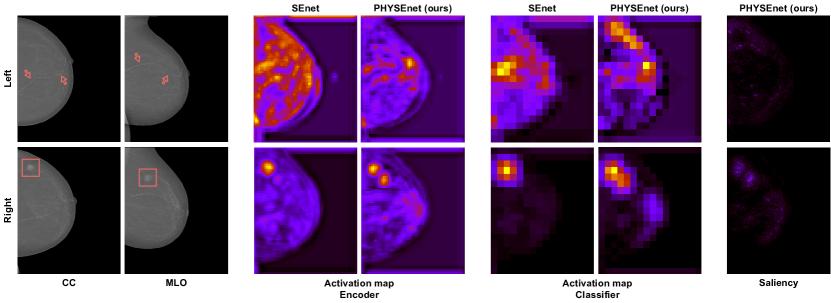
Figure 5: From the left, a sample exam from the INbreast dataset containing a benign calcification on the left side and a malignant mass on the right side. Then, activation maps to visualize the learned latent representations of PHYSEnet and SEnet at encoder and classifier level. Lastly, the saliency map for PHYSEnet containing the most relevant pixels according to the gradient.

For this set of experiments, we consider one of the official tasks of the BraTS19 challenge [47], which is the prediction of the overall survival (OS) in the number of days from each patient. The task evaluation is done considering three different classes: short-term (less than 10 months), mid-term (between 10 and 15 months), and long-term (more than 15 months) survivors. The input of the model comprises the volumes corresponding to modalities T2 and FLAIR and the age of the patient. Thus, for this case, we define and employ 3D parameterized hypercomplex convolutions to process the volumes, specifically PHResNet3D, and a linear layer for the age input. Then, the learned features are summed together [48] and processed by two linear layers to produce the final output. The experiment results in Tab. VI prove the flexibility of the method with respect to a different task and input, as the hypercomplex network yields 56.3% accuracy, far exceeding the respective model in the real domain. Importantly, these results also show that the proposed architectures can not only learn good representations from different views, i.e. a different angle of the same subject, but also from multiple modalities, i.e. the same view but containing different information.

VI-D3 Multimodal brain tumor segmentation

Lastly, in this section, we demonstrate how this framework can easily be extended for different tasks and employed with any network architecture. To this end, we conduct experiments regarding brain tumor segmentation from multimodal slices extracted from MRI volumes. We define the more appropriate UNet [52] in the hypercomplex domain, i.e. PHUNet, and set the parameter $n=2$ considering the same modalities as for the OS prediction. The two models in the real and hypercomplex domain yield a very similar Dice score average of about $83\%$ on BraTS19 [41], as reported in Tab. VII, proving the validity of the proposed approach also for finer-scaled tasks. Moreover, we believe these results can be further improved in future works that mainly focus on tasks such as detection and segmentation, employing more complex networks and extending to a 3D segmentation scenario.

VI-E Ablation Study

The most relevant ablation studies for the proposed architectures are actually already included in previous experiments reported in Section VI. As an example, an interesting ablation study is to remove significant parts from the different networks. In that sense, the most crucial network modules are represented by the PHC layers. Removing the potential of parameterized hypercomplex operations, the model turns out to be equivalent to its real-valued counterpart. However, we have shown in Subsection VI-B2 and Subsection VI-C2 that the hypercomplex networks greatly outperform the respective real-valued counterparts for each proposed model. Those results prove how the gain in performance is owed to the capabilities to exploit multi-view correlations that are endowed to our methods thanks to the introduction of hypercomplex algebra in a convolutional layer.

In Tab. III, we have additionally shown the impact of the deployed pretraining strategy: randomly initializing networks weights leads to poor performance, because tumor masses or calcifications are arduous to detect, and even more to classify, from the original mammogram, as they occupy a tiny portion of the image. On the contrary, thanks to the pretraining recipe we adopt, the fine-grained detail characteristic of high-resolution mammograms is leveraged as a result of the patch classifier and effectively transferred for learning with entire mammogram images.

TABLE VII: Results for brain tumor segmentation on BraTS19.

Model	Params	Dice Score
UNet	31M	0.826 $\pm$ 0.017
PHUNet	15M	0.825 $\pm$ 0.018

VII Visualizing multi-view learning

TABLE VIII: Models use cases summary. The ticks ✓ mean that the model can be adopted in the specific case if our pretrained weights are employed. This is because without ROI annotations it is not possible to train a patch classifier, thus the pretraining stage cannot be performed.

Use Cases	PHResNet18	PHResNet50	PHYBOnet	PHYSEnet
Single View	✓	✓	✗	✗
Two Views	✓	✓	✗	✗
Four Views	✗	✗	✓	✓
ROI available	✓	✓	✓	✓
ROI not available	✓	✓	✓	✓
Light memory	✓	✗	✓	✗
Small size dataset	✓	✓	✓	✓
Other problems	✓	✓	✓	✓

To further assess the crucial role of multi-view learning in breast cancer classification, here we provide a visual explanation of PHYSEnet results, comparing it against its real-valued counterpart, displayed in Fig. 5.

We consider a patient from INbreast with a benign finding in the left breast and a malignant mass in the right breast. In order to obtain a visual representation of what the model has learned, we compute activation maps by taking the average of the feature channels. Specifically, we acquire activation maps at two levels of the architecture, that is at the output of the shared encoder and at the output of the refiner blocks (classifier). Regarding the left views, by observing the activation maps of PHYSEnet, especially at the encoder level, we can see how it has learned a more focused representation, as the regions corresponding to the benign calcification are highlighted. While in the maps of SEnet, all areas of the breast are accentuated. But most importantly, by comparing the maps of the right view obtained from the model in the real domain and the hypercomplex domain, we can discern a crucial point. Indeed, in the input images, the mass is clearly visible in both CC and MLO views. However, if the two views are overlapped the mass does not align, as it should since the images give a different view of the breast. From the activation maps of PHYSEnet, it is clear that the network is learning from both views, as two areas are highlighted, corresponding to the location of the mass in the CC view and the MLO view. On the other hand, in the activation maps of SEnet, only one highlighted area appears, corresponding to the CC view only. Thus, it seems that the real model is relying on the CC view only, not considering and exploiting the MLO view, like the PH model is doing. Therefore, the real model is not truly leveraging both views but is relying on a single view. Moreover, sometimes a mass is visible only in one of the two views. Thus, if the network has learned to rely only on the CC view and the mass is visible only on the MLO view, the mass will not be detected.

Finally, for the hypercomplex network, we additionally obtain the saliency maps in order to visualize which area of the two-view input is most influential for the model decision. Also in this case, for the right side, we can observe the highlighted pixels that indeed correspond to the malignant mass, while the left-side map is darker and no pixel region is particularly accentuated since there are no malignant findings in the left breast. Interestingly, the maps for the left side differ between activation maps and saliency maps. This point highlights how the learned representation, visualized as activation maps, leverages patient-level information, i.e. from both sides, while the classification decision visualized in the saliency map has no highlighted area as the left view is classified as benign.

VIII How do I choose the best model for my data?

In this section, we aim at answering the reader question Which model do I employ on my data and for my problem?

We consider multiple scenarios, including datasets with 1, 2, or 4 views, whether ROI annotations are available or not, the memory constraints, the size of the dataset, and if proposed models are easily exportable to other kinds of medical imaging problems. Table VIII reports the applicability of each network we propose in the above-mentioned scenarios. Moreover, while we prove the crucial role of pretraining for breast cancer classification tasks, especially when only scarce data is available, this is only applicable in the case of datasets with provided ROI annotations. Nevertheless, our methods can be applied even in datasets where ROI observations are missing, since we provide pretrained models and weights to overcome this limitation. We believe that Table VIII may help the reader clarify which model better fits specific cases and may increase the usability of our approach in future research and in different medical fields.

IX Conclusions

In this paper, we have introduced an innovative approach for breast cancer classification that handles multi-view mammograms as a radiologist does, thus leveraging information contained in ipsilateral views as well as bilateral. Thanks to hypercomplex algebra properties, neural models are endowed with the capability of capturing and truly exploiting correlations between views and thus outperforming state-of-the-art models. At the same time, we demonstrate how our approach generalizes considering different imaging exams as well as proving its efficacy on finer-scaled tasks, while also being flexible to be adopted in any existing neural network. On a thorough evaluation on publicly available benchmark datasets, we have shown the improved AUC and accuracy values of the proposed approach with respect to state-of-the-art methods, together with greater robustness of such results. We believe that our approach is a real breakthrough for this research field and that it may pave the way to novel methods capable of processing medical imaging exams with techniques closer to radiologists and to human understanding.

References

- [1] R. L. Siegel, K. D. Miller, H. E. Fuchs, and A. Jemal, “Cancer statistics, 2022,” CA: A Cancer Journal for Clinicians, vol. 72, no. 1, pp. 7–33, 2022.
- [2] I. C. Moreira, I. Amaral, I. Domingues, A. Cardoso, M. J. Cardoso, and J. S. Cardoso, “INbreast: Toward a full-field digital mammographic database,” Academic Radiology, vol. 19, no. 2, pp. 236–248, 2012.
- [3] S. Misra, N. L. Solomon, F. L. Moffat, and L. G. Koniaris, “Screening criteria for breast cancer,” Adv. Surg., vol. 44, pp. 87–100, 2010.
- [4] D. Gur, G. S. Abrams, D. M. Chough, M. A. Ganott, C. M. Hakim, R. L. Perrin, G. Y. Rathfon, J. H. Sumkin, M. L. Zuley, and A. I. Bandos, “Digital breast tomosynthesis: Observer performance study,” American Journal of Roentgenology, vol. 193, no. 2, pp. 586–591, 2009.
- [5] Y. Liu, F. Zhang, C. Chen, S. Wang, Y. Wang, and Y. Yu, “Act like a radiologist: Towards reliable multi-view correspondence reasoning for mammogram mass detection,” IEEE Trans. Pattern Anal. Mach. Intell., no. 01, pp. 1–1, 2021.
- [6] L. Shen, L. Margolies, J. Rothstein, E. Fluder, R. McBride, and W. Sieh, “Deep learning to improve breast cancer detection on screening mammography,” Sci. Rep., vol. 9, 2019.
- [7] N. Wu, Z. Huang, Y. Shen, J. Park, J. Phang, T. Makino, S. Kim, K. Cho, L. Heacock, L. Moy, and K. J. Geras, “Reducing false-positive biopsies using deep neural networks that utilize both local and global image context of screening mammograms,” Journal of Digital Imaging, vol. 34, pp. 1414 – 1423, 2021.
- [8] G. Murtaza, L. Shuib, A. Wahid, G. Mujtaba, H. Nweke, M. Al-Garadi, F. Zulfiqar, G. Raza, and N. Azmi, “Deep learning-based breast cancer classification through medical imaging modalities: state of the art and research challenges,” Artificial Intelligence Review, vol. 53, 03 2020.
- [9] D. Abdelhafiz, C. Yang, R. Ammar, and S. Nabavi, “Deep convolutional neural networks for mammography: advances, challenges and applications,” BMC Bioinformatics, vol. 20, 2019.
- [10] S. S. Aboutalib, A. A. Mohamed, W. A. Berg, M. L. Zuley, J. H. Sumkin, and S. Wu, “Deep Learning to Distinguish Recalled but Benign Mammography Images in Breast Cancer Screening,” Clinical Cancer Research, vol. 24, no. 23, pp. 5902–5909, 2018.
- [11] I. Sechopoulos and M. R. Mann, “Stand-alone artificial intelligence - the future of breast cancer screening?” The Breast, vol. 49, pp. 254–260, 2020.
- [12] M. A. Al-antari, M. A. Al-masni, and T.-S. Kim, “Deep learning computer-aided diagnosis for breast lesion in digital mammogram,” Adv. Exp. Med. Biol., vol. 1213, pp. 59–72, 2020.
- [13] R. Agarwal, O. Diaz, X. Lladó, M. H. Yap, and R. Martí, “Automatic mass detection in mammograms using deep convolutional neural networks,” Journal of Medical Imaging, vol. 6, no. 3, pp. 1–9, 2019.
- [14] J. Niu, H. Li, C. Zhang, and D. Li, “Multi-scale attention-based convolutional neural network for classification of breast masses in mammograms,” Medical Physics, vol. 48, no. 7, pp. 3878–3892, 2021.
- [15] G. Zhao, Q. Feng, C. Chen, Z. Zhou, and Y. Yu, “Diagnose like a radiologist: Hybrid neuro-probabilistic reasoning for attribute-based medical image diagnosis,” IEEE Trans. Pattern Anal. Mach. Intell., 2021.
- [16] H. Pinckaers, B. van Ginneken, and G. Litjens, “Streaming convolutional neural networks for end-to-end learning with multi-megapixel images,” IEEE Trans. Pattern Anal. Mach. Intell., vol. 44, no. 3, pp. 1581–1590, 2022.
- [17] C. Lian, M. Liu, J. Zhang, and D. Shen, “Hierarchical fully convolutional network for joint atrophy localization and alzheimer’s disease diagnosis using structural MRI,” IEEE Trans. Pattern Anal. Mach. Intell., vol. 42, no. 4, pp. 880–893, 2020.
- [18] N. Wu, J. Phang, J. Park, Y. Shen, Z. Huang, M. Zorin, S. Jastrzebski, T. Fevry, J. Katsnelson, E. Kim, S. Wolfson, U. Parikh, S. Gaddam, L. Lin, K. Ho, J. Weinstein, B. Reig, Y. Gao, H. Toth, K. Pysarenko, A. Lewin, J. Lee, K. Airola, E. Mema, S. Chung, E. Hwang, N. Samreen, S. Kim, L. Heacock, L. Moy, K. Cho, and K. Geras, “Deep neural networks improve radiologists’ performance in breast cancer screening,” IEEE Trans. Med. Imaging, vol. 39(4), 2020.
- [19] N. Wu, S. Jastrzębski, J. Park, L. Moy, K. Cho, and K. Geras, “Improving the ability of deep neural networks to use information from multiple views in breast cancer screening,” in Proc. of the Third Conf. on Med. Imaging with Deep Learning, vol. 121. PMLR, 2020, pp. 827–842.
- [20] C. Zhang, J. Zhao, J. Niu, and D. Li, “New convolutional neural network model for screening and diagnosis of mammograms,” PLoS ONE, vol. 15(8), 2020.
- [21] T. Kyono, F. J. Gilbert, and M. van der Schaar, “Mammo: A deep learning solution for facilitating radiologist-machine collaboration in breast cancer diagnosis,” arXiv preprint: arXiv:1811.02661, 2018.
- [22] ——, “Triage of 2d mammographic images using multi-view multi-task convolutional neural networks,” ACM Trans. Comput. Healthcare, vol. 2, no. 3, 2021.
- [23] ——, “Multi-view multi-task learning for improving autonomous mammogram diagnosis,” in Proceedings of the 4th Machine Learning for Healthcare Conference, ser. Proceedings of Machine Learning Research, vol. 106. PMLR, 2019, pp. 571–591.
- [24] L. Sun, J. Wang, Z. Hu, Y. Xu, and Z. Cui, “Multi-view convolutional neural networks for mammographic image classification,” IEEE Access, vol. 7, pp. 126 273–126 282, 2019.
- [25] J. Song, Y. Zheng, M. Z. Ullah, J. Wang, Y. Jiang, C. Xu, Z. Zou, and G. Ding, “Multiview multimodal network for breast cancer diagnosis in contrast-enhanced spectral mammography images,” International Journal of Computer Assisted Radiology and Surgery, vol. 16, pp. 979 – 988, 2021.
- [26] G. Carneiro, J. C. Nascimento, and A. P. Bradley, “Unregistered multiview mammogram analysis with pre-trained deep learning models,” in Int. Conf. on Medical Image Computing and Computer Assisted Intervention (MICCAI), 2015.
- [27] J. Ma, X. Li, H. L., Ruixuan, W. Ruixuan, B. Menze, and W. Zheng, “Cross-View relation networks for mammogram mass detection,” in 2020 25th International Conference on Pattern Recognition (ICPR), 2021, pp. 8632–8638.
- [28] Z. Yang, Z. Cao, Y. Zhang, Y. Tang, X. Lin, R. Ouyang, M. Wu, M. Han, J. Xiao, L. Huang, S. Wu, P. Chang, and J. Ma, “MommiNet-v2: Mammographic multi-view mass identification networks,” Medical Image Analysis, vol. 73, p. 102204, 2021.
- [29] T. Baltrušaitis, C. Ahuja, and L.-P. Morency, “Multimodal machine learning: A survey and taxonomy,” IEEE Trans. Pattern Anal. Mach. Intell., vol. 41, no. 2, pp. 423–443, 2019.
- [30] W. Wang, D. Tran, and M. Feiszli, “What makes training multi-modal classification networks hard?” in 2020 IEEE/CVF Conf. on Computer Vision and Pattern Recognition (CVPR), 2020, pp. 12 692–12 702.
- [31] C. Gaudet and A. Maida, “Deep quaternion networks,” in IEEE Int. Joint Conf. on Neural Netw. (IJCNN), Rio de Janeiro, Brazil, Jul. 2018.
- [32] T. Parcollet, M. Morchid, and G. Linarès, “A survey of quaternion neural networks,” Artif. Intell. Rev., Aug. 2019.
- [33] T. Parcollet, M. Ravanelli, M. Morchid, G. Linarès, C. Trabelsi, R. De Mori, and Y. Bengio, “Quaternion recurrent neural networks,” in Int. Conf. on Learning Representations (ICLR), New Orleans, LA, May 2019, pp. 1–19.
- [34] D. Comminiello, M. Lella, S. Scardapane, and A. Uncini, “Quaternion convolutional neural networks for detection and localization of 3D sound events,” in IEEE Int. Conf. on Acoust., Speech and Signal Process. (ICASSP), Brighton, UK, May 2019, pp. 8533–8537.
- [35] M. Ricciardi Celsi, S. Scardapane, and D. Comminiello, “Quaternion neural networks for 3D sound source localization in reverberant environments,” in IEEE Int. Workshop on Machine Learning for Signal Process., Espoo, Finland, Sep. 2020, pp. 1–6.
- [36] C. Brignone, G. Mancini, E. Grassucci, A. Uncini, and D. Comminiello, “Efficient sound event localization and detection in the quaternion domain,” IEEE Trans. on Circuits and Systems II: Express Brief, vol. 69, no. 5, pp. 2453–2457, 2022.
- [37] A. Zhang, Y. Tay, S. Zhang, A. Chan, A. T. Luu, S. C. Hui, and J. Fu, “Beyond fully-connected layers with quaternions: Parameterization of hypercomplex multiplications with parameters,” Int. Conf. on Machine Learning (ICML), 2021.
- [38] E. Grassucci, A. Zhang, and D. Comminiello, “PHNNs: Lightweight neural networks via parameterized hypercomplex convolutions,” arXiv preprint: arXiv:2110.04176, 2021.
- [39] R. Lee, F. Gimenez, A. Hoogi, M. Kanae, M. Gorovoy, and D. Rubin, “A curated mammography data set for use in computer-aided detection and diagnosis research,” Sci. Data, vol. 4, 2017.
- [40] J. e. a. Irvin, “CheXpert: A large chest radiograph dataset with uncertainty labels and expert comparison,” in Proceedings of the AAAI conference on artificial intelligence, vol. 33, no. 01, 2019, pp. 590–597.
- [41] B. H. e. a. Menze, “The multimodal brain tumor image segmentation benchmark (BRATS),” IEEE Trans. on Med. Imaging, no. 10, pp. 1993–2024, 2015.
- [42] S. Bakas, H. Akbari, A. Sotiras, M. Bilello, M. Rozycki, J. S. Kirby, J. B. Freymann, K. Farahani, and C. Davatzikos, “Advancing the cancer genome atlas glioma MRI collections with expert segmentation labels and radiomic features,” Scientific data, vol. 4, no. 1, pp. 1–13, 2017.
- [43] M. E. Valle and R. A. Lobo, “Hypercomplex-valued recurrent correlation neural networks,” Neurocomputing, vol. 432, pp. 111–123, 2021.
- [44] E. Grassucci, E. Cicero, and D. Comminiello, “Quaternion generative adversarial networks,” in Generative Adversarial Learning: Architectures and Applications, R. Razavi-Far, A. Ruiz-Garcia, V. Palade, and J. Schmidhuber, Eds. Cham: Springer International Publishing, 2022, pp. 57–86.
- [45] M. Raghu, C. Zhang, J. Kleinberg, and S. Bengio, “Transfusion: Understanding transfer learning for medical imaging,” in Proceedings of the 33rd International Conference on Neural Information Processing Systems (NIPS), 2019, p. 3347–3357.
- [46] K. Geras, S. Wolfson, S. Kim, L. Moy, and K. Cho, “High-resolution breast cancer screening with multi-view deep convolutional neural networks,” arXiv preprint: arXiv:1703.07047, 2017.
- [47] S. e. a. Bakas, “Identifying the best machine learning algorithms for brain tumor segmentation, progression assessment, and overall survival prediction in the BRATS challenge,” arXiv preprint arXiv:1811.02629, 2018.
- [48] R. Hermoza, G. Maicas, J. C. Nascimento, and G. Carneiro, “Post-hoc overall survival time prediction from brain MRI,” in IEEE 18th Int. Symp. on Biom. Imag. (ISBI), 2021, pp. 1476–1480.
- [49] D. P. Kingma and J. Ba, “Adam: A method for stochastic optimization,” in 3rd International Conference on Learning Representations, ICLR 2015, San Diego, CA, USA, May 7-9, 2015, Conference Track Proceedings, Y. Bengio and Y. LeCun, Eds., 2015. [Online]. Available: http://arXiv.org/abs/1412.6980
- [50] K. He, X. Zhang, S. Ren, and J. Sun, “Deep residual learning for image recognition,” in IEEE/CVF Conf. on Computer Vision and Pattern Recognition (CVPR), 2016, pp. 770–778.
- [51] J. Rubin, D. Sanghavi, C. Zhao, K. Lee, A. Qadir, and M. Xu-Wilson, “Large scale automated reading of frontal and lateral chest x-rays using dual convolutional neural networks,” arXiv preprint: arXiv:1804.07839, 2018.
- [52] O. Ronneberger, P. Fischer, and T. Brox, “U-net: Convolutional networks for biomedical image segmentation,” in Medical Image Computing and Computer-Assisted Intervention (MICCAI). Springer International Publishing, 2015, pp. 234–241.