Coarse Personalization

Abstract

Advances in estimating heterogeneous treatment effects enable firms to personalize marketing mix elements and target individuals at an unmatched level of granularity, but feasibility constraints limit such personalization. In practice, firms choose which unique treatments to offer and which individuals to offer these treatments with the goal of maximizing profits: we call this the coarse personalization problem. We propose a two-step solution that makes segmentation and targeting decisions in concert. First, the firm personalizes by estimating conditional average treatment effects. Second, the firm discretizes by utilizing treatment effects to choose which unique treatments to offer and who to assign to these treatments. We show that a combination of available machine learning tools for estimating heterogeneous treatment effects and a novel application of optimal transport methods provides a viable and efficient solution. With data from a large-scale field experiment for promotions management, we find that our methodology outperforms extant approaches that segment on consumer characteristics or preferences and those that only search over a prespecified grid. Using our procedure, the firm recoups over $99.5\%$ of its expected incremental profits under fully granular personalization while offering only five unique treatments. We conclude by discussing how coarse personalization arises in other domains.

Keywords: Personalization, Targeting, Segmentation, Optimal Transport, Machine Learning

1 Introduction

Developments in heterogeneous–treatment effects estimation techniques enable firms to target customers close to the individual level. The state of the art personalized marketing technology leverages machine learning to form granular segments wherein a customer with a set of unique covariates can constitute a segment by herself. Such granular segmentation and targeting approaches allow marketers to construct personalized targeting regimes where only customers who generate positive incremental profits for the firm are targeted (Hitsch et al., 2023; Ascarza, 2018; Yoganarasimhan et al., 2022; Dube and Misra, 2022; Athey and Wager, 2021). Consequently, marketing decisions are profit maximizing because individuals are targeted only when the marginal benefit outweighs the marginal cost of targeting.

However, these personalization and targeting procedures can face barriers in practice. Examples include the costs of managing a large portfolio of offers or menu costs (Sheshinski and Weiss, 1977), issues pertaining to inequity or fairness (Kahneman et al., 1986), and possible antitrust concerns (OECD, 2018). The trade press often points to the complexities of implementing personalized policies with particular focus on the high costs of setting up the infrastructure to conduct such personalization. Recent privacy regulations effectively add an additional barrier to full personalization by limiting the data that firms can use to personalize their offerings.

Given these constraints, it is not surprising that firms may wish to restrict the set of unique marketing treatments to offer. Consequently they are faced with the decision of which customers to assign to these treatments. In essence, firms need to create smaller sets, or segments, of customers and optimally choose treatments for each set with the aim of maximizing profits. We call this problem the coarse personalization problem.

The coarse personalization problem is not entirely new. Marketing has long understood the need to segment consumers with the idea of personalizing the marketing mix to each segment while also keeping the costs of such personalizing within bounds. The typical process is sequential, and we first group customers into segments and then personalizing the marketing treatments or offers for segments that we wish to target. Indeed, the textbook approach is to implement an “discretize then personalize” framework where we form customer segments based on some pre-defined source of customer heterogeneity, identify which segments we wish to target, and then tailor marketing mix variables for each segment (Kotler and Keller, 2014). Over time, the sources of customer heterogeneity that underpins the segmentation procedure has evolved. Initially, marketing researchers proposed forming segments on demographic and psychographic variables such as on household size and income (Smith, 1956; Wind, 1978; Gupta and Chintagunta, 1994). More recently, researchers form segments based on estimated consumer preferences (Kamakura and Russell, 1989; Bucklin and Gupta, 1992; Bucklin et al., 1998) via either continuous or discrete mixtures (Grover and Srinivasan, 1987; Jain et al., 1990).

In practice, the “discretize then personalize” framework is used quite broadly in marketing but especially in the customer relationship management (CRM), database and direct marketing literatures where marketers form segments first and then make targeting decisions conditional on the segments. In the CRM literature, Reinartz and Kumar (2003) consider forming segments based on recency, frequency, monetary value (RFM) and demographic variables, and Verhoef (2003) demonstrates the response heterogeneity of customers to multiple marketing interventions. Rust and Verhoef (2005) study the performance of various segmentation models for different CRM interventions in generating intermediate profits for the firm. They find that a Bayesian hierarchical model that incorporates customer demographics and RFM behavior performs better than finite mixture models and models that segment ex ante on demographics and RFM covariates. While the literature has evolved considerably in terms of the information it uses, the structure of the framework and the sequence of steps has remained essentially the same.

In this paper, we show that implementing these steps separately in the prescribed sequence is not necessarily profit maximizing. This is primarily because of the fact that the segmentation procedure is based on a distance metric that statistical (e.g. Euclidian) rather than economic in nature (profits). To address this problem we recharacterize the coarse personalization problem as an optimal transport problem and derive a theoretically rigorous yet practically implementable solution. In doing so, we draw on modern machinery from the incrementality-based targeting literature as well as new developments in the optimal transport literature. In particular, we advocate for a “personalize then discretize” approach where we first construct personalized policies based on heterogeneous treatment effects obtained using now widely available machine learning (ML) tools, and in a second step, we use these policies to construct segments of consumers by minimizing profit regret. Crucially, in the second step we are simultaneously identifying each segment’s treatment policy (what to offer) as well as the assignment protocol (who to offer it to) that allocates individual customers to a segment to maximize profits. Put simply, this approach inverts the “discretize then personalize” approach by first searching for what works for each customer and then deciding on a coarsened marketing mix offering that would not degrade profits significantly relative to full personalization.

Our two-step framework solves the coarse personalization problem precisely because it is able to segment consumers based on a profit-relevant distance metric. As such, we view our key contribution to be the design of the second step that allows for the construction and implementation of this solution. The first step’s ML-based personalization, done by exploiting heterogeneous treatment effects, is now relatively straightforward from the literature. On the other hand, the issue of coarsening these to satisfy the problem poses challenges on multiple fronts. The combinatorial nature of the assignment problem coupled with the optimization of the treatment policy makes the problem especially difficult. Our proposed solution coarsens the treatment policy to account for the constraint that policy space is limited to contain only a finite number of unique treatments. This done using optimal transport methods that minimize the regret between the profits that accrue from the full personalization solution to those from any proposed coarsened solution. The regret minimizing solution guarantees that we attain the highest possible profits while incorporating the additional constraint on the number of treatments available.

Our framework adapts semidiscrete optimal transport theory that formalizes the problem of mapping moving mass from a continuous measure to a discrete one to minimize some pre-defined cost. In the context of the marketing problem that we face, after the first step is completed, the firm knows exactly how much profit it can make from a fully granular personalization scheme. This acts as a benchmark for our second step: the optimal transport machinery allows us to form segments and their treatments simultaneously with the aim of getting as close to the profits under fully granular personalization as possible. We show that the optimal transport problem is a strictly convex optimization problem in the assigned treatment values and consequently, at the optimal solution, the average marginal effect of the treatment is equated to the marginal cost of the treatment for each assigned segment.

To be clear, while one might be able to solve the coarse personalization problem by brute force, the complexity of the problem is exponential in the number of people and suffers from the curse of dimensionality. Instead, we propose a computational solution that adapts Lloyd’s Algorithm (Lloyd, 1982) and leverages the convexity of the problem. Our adapted version of Lloyd’s Algorithm is scalable, provides a transparent visualization of the solution’s procedure, and is computationally much faster. Other algorithms to solve optimal transport problems are detailed in Peyré and Cuturi (2019) and can be adapted to solve our coarse personalization problem.

In our empirical application, we find that our solution significantly outperforms traditional marketing procedures that segment on demographics, RFM variables, and consumer preferences in generating profits for promotions management for a food delivery platform. Further, we find that if the firm issues only five unique optimized treatments, our solution recovers over $99.5\%$ of the fully granular personalization’s expected incremental profits. We also illustrate the extent to which our “personalize then discretize” approach outperforms the traditional “discretize then personalize” approach by comparing our solution to classical marketing benchmarks.

In an additional analysis we document the impact personalization has on consumer and producer surplus as the firm moves from coarse policies (with a few optimally chosen treatments) to fully granular personalization. Bergemann and Bonatti (2011) theoretically find that as the firm is able to target more granularly, producer surplus increases along with the total surplus. Dube and Misra (2022) find that consumer surplus changes nonmonotonically as firms are able to target more granularly. Using our coarse personalization framework, we empirically examine the surplus implications as the firm increases its ability to granularly target. Coarser targeting reduces producer surplus due to the extra constraint on the firm’s problem, but it can increase consumer surplus for some individuals because they may be given a higher or lower level of treatment than what they would have gotten under the fully granular personalization scenario. Like in the aforementioned research, we document that the impact of personalization on consumer welfare is not unambiguous and needs further study.

Lastly, we discuss how the coarse personalization problem naturally arises in other traditional marketing contexts. In salesforce contract design, managers need to determine which geographic blocks for salespeople to exert effort in, how much time to spend, and whether to call or visit in person. Advertising designers need to choose which set of advertisements and their characteristics to send out to customers. Pricing managers can choose to use nudges or price subsidies to influence consumer behavior. All of these marketing problems can be tackled with our coarse personalization framework.

The application in our paper also contributes to the literature on promotions management. Personalization and customization using price promotions is a classical marketing problem and promotions are personalized based on customer heterogeneity (Rossi et al., 1996; Shaffer and Zhang, 1995). With the advent of online marketplaces, promotions are more readily personalized, customized, and distributed to customers (Ansari and Mela, 2003; Zhang and Krishnamurthi, 2004). The optimization approach to promotions management has been explored in the literature (Duvvuri et al., 2007; Zhang and Wedel, 2009), but often promotions are optimized after forming the customer segments following the traditional marketing framework. Most recently, marketers have used tools from causal machine learning with online databases to target and personalize promotions based on their heterogeneous treatment effects (Rafieian and Yoganarasimhan, 2021; Ellickson et al., 2022; Yoganarasimhan et al., 2022; Hitsch et al., 2023). Our framework combines the classical optimization approach with the more modern approach of using heterogeneous treatment effects, and we provide an empirical example of our approach for promotions management.

Additionally, our paper provides a novel application of the optimal transport literature to the marketing literature. Optimal transport problems have been applied to discrete choice models under the mass transport framework (Chiong et al., 2016; Bonnet et al., 2017), matching markets (Galichon and Salanie, 2012), quantile regression (Carlier et al., 2016), bounding regression discontinuity design estimates (Daljord et al., 2019), and its general applications to economics are surveyed in (Galichon, 2016). Computational methods for evaluating optimal transport problems are detailed in (Peyré and Cuturi, 2019) and a survey of recent mathematical developments in the field can be found in Villani (2009).

The next section of the paper overviews our solution’s methodology to the coarse personalization problem. Section 3 of the paper formulates our solution to the problem: the first step is described in Section 3.1 and the second step is fleshed out in Section 3.2. The empirical application of promotions management for a large food delivery firm is provided in Section 4. The surplus analysis is discussed in Section 5. We discuss how our framework can be adopted to address other classic marketing problems in Section 6.

2 Methodological overview

To put this paper’s methodological insight simply, when marketers “personalize then discretize”, which means to form segments and marketing mix variables in concert, they are more likely to be profit maximizing. We first show how this approach provides an upper bound for profits to the classical marketing approach that “discretizes then personalizes” and that forms segments and chooses each assigned treatment sequentially rather than simultaneously. We then note that solving the two components simultaneously is difficult in practice, which motivates our recasting of the problem in an optimal transport framework.

To show that maximizing segments and their assigned treatments simultaneously rather than sequentially is more profit maximizing, we consider the following stylized example. Individuals have covariate characteristics $\boldsymbol{x}_{i}$, and we denote $S(\boldsymbol{x}_{i})$ to be the function that assigns individuals to segments and $T(S(\boldsymbol{x}_{i}),\boldsymbol{x}_{i})$ to be the function that maps segments to their assigned treatment.

The classical sequential approach forms segments based on consumer characteristics and/or preferences (Kotler and Keller, 2014). More generally, we consider any form of a priori segmentation and denote it by $S^{0}(\boldsymbol{x}_{i})$. After segments are formed, the marketer then solves for the optimal treatment values $T(S^{0}(\boldsymbol{x}_{i}),\boldsymbol{x}_{i})$ taking the a priori segmentation as given.

In contrast, our approach solves the two problems in concert. We first define profits as $\Pi(S(\boldsymbol{x}_{i}),T(\boldsymbol{x}_{i},S))$ and then the simultaneous solution solves for segmentation $S$ to maximize profits and chooses treatments by $T(S(\boldsymbol{x}_{i}),\boldsymbol{x}_{i})$ to maximize profits.

The simultaneous approach provides an upper bound in profits compared to the sequential approach,

$$\max_{S,T}\Pi(S,T(S))\geq\max_{T}\Pi(S^{0},T(S^{0}))$$ (1)

where we suppressed the dependence on $\boldsymbol{x}_{i}$ in our notation and $S^{0}$ represents the a priori segmentation from the classical approach. The left-hand side in Equation 1 represents the profits from the simultaneous approach where the profits are maximized to both arguments. The right-hand side represents sequential approach where treatments are chosen only after segments $S^{0}$ are formed. The inequality holds by the property of the maximization operator over $S$. The inequality will bind only if the a priori segmentation is ex post optimal for profit maximization or equivalently when $S^{0}\in\operatorname*{argmax}_{S^{\prime}}\max_{T}\Pi(S^{\prime},T(S^{\prime}))$. Hence, the simultaneous approach that we propose in this paper will be an upper bound for any sequential segmentation procedure. In our empirical application, we evaluate our simultaneous approach to different sequential benchmarks used in classical marketing in Section 4.3.1.

While our simultaneous approach is more profitable, solving it in practice is quite difficult. Using the promotions management setting from our empirical example, if we decide to form three unique segments that are each assigned a promotion that can take on ten different different dollar off or percentage off values for fifteen people, the total number of combinations is ${10\times 2\choose 3}3^{15}$, which is over $16$ billion combinations. Even in this small example, we see that the space over which to search over is combinatorially large and for more modern digital marketing applications with many treatment arms that are issued to millions of customers, the problem only gets substantially more complex.

Modern approaches attempt to solve the problem by A/B testing each discrete treatment arm, evaluating the heterogeneous treatment effects, and forming segments among the extant treatment arms to maximize profits (Hitsch et al., 2023). In our running example in promotions management, we have ten different values tested for both dollar and percentage off promotions. This means we have twenty treatment arms to evaluate heterogeneous treatment effects. Segments are then formed by assigning individuals to their best offered treatment arm.

In this modern approach, the continuity of the treatments themselves is ignored. In our application, this means the dollar off and percentage off promotions are treated as discrete instead of as continuous. Ignoring the continuity of the treatments leads has two implications: First, the choice of which segments to offer is still combinatorially large and suffers from the curse of dimensionality. In our running example, to offer three segments, the marketer needs to search over ${10\times 2\choose 3}=1,140$ different treatment offering combinations. In another example with five marketing mix variables that can take ten discrete values each, the marketer would need to search over ${10\times 5\choose 3}=19,600$ different treatment offering combinations to form three distinct segments. Second, because many marketing mix variables, such as price, promotional value, and product attributes, are continuous, when a firm only looks at discrete values, it forgoes possible profits by not considering values between the discrete values tested in the A/B testing experiment. Section 4.3.2 benchmarks the modern A/B Testing approach in our empirical application and documents the loss in profits by ignoring the continuity of the treatment effects.

To mitigate the complexity of the problem and to provide a scalable solution, we consider the treatments to be continuous and leverage tools from optimal transport and convex analysis. We show that (1) the segmentation problem can be written as an semidiscrete optimal transport step, where we map individuals to segments, and (2) the problem of solving for the optimal treatments to offer is convex in the treatment values.

However, we make two conventional assumptions to ensure the problem is tractable. First, we assume that individuals have diminishing sensitivity in each type of treatment, i.e., people are less sensitive to changes at higher dollar off promotion values. Second, we assume the firm’s cost function for issuing higher levels of promotions has no economies of scale, i.e., the firm does not have lower marginal cost at higher levels of the promotional value. These two assumptions afford us the convexity of the simultaneous problem in the left-hand side of Equation 1 and ensure each individual is deterministically assigned to a segment. We flesh out the details of our methodology in the next section.

3 Model

Our approach incorporates two steps to solve the coarse personalization problem. The first is to estimate treatment effects in a randomized control trial (RCT) setting using tools from the heterogeneous treatment effects and continuous treatments literatures. The second is to choose which treatments to offer and who to assign to each treatment using an optimal transport framework. The first step is described in Section 3.1 and the second step is fleshed out in Section 3.2. We emphasize that the second step is a novel application of optimal transport and the first step itself is presently used for fully granular incrementality-based targeting. We provide a overview of the mathematics of our second step in the Appendix Section A.

For each individual $i$ with covariate vector $\boldsymbol{x}_{i}$, we estimate continuous treatment effects for each dimension $d$ of treatment. The firm is then given a number of unique treatments $L$ that are non-zero in only one dimension $d\in\{1,\ldots,D\}$ and chooses (1) which treatments to offer and (2) the assignment of individuals $i$ to each treatment $l\in L$.

For individual $i\in\{1,\ldots,N\}$, we denote the individual characteristics as $\boldsymbol{x}_{i}$ and the firm’s outcome measure as $Y_{i}$. Treatments are finite $D$-dimensional, and the treatment vector for individual $i$ is denoted as,

$$\boldsymbol{t}_{i}=(t_{i,1},\ldots,t_{i,d},\ldots,t_{i,D})$$ (2)

where $t_{i,d}$ is the treatment level in dimension $d$. The feasible set of treatments available to the firm are non-zero only in one dimension and have the format $(0,\ldots,t_{i,d},\ldots,0)$ where $t_{i,d}\neq 0$. A vector of zeros for $\boldsymbol{t}_{i}$ represents the no treatment case.

The cost of treatment $\boldsymbol{t}_{i}$ is $c_{i}(t_{i,1},\ldots,t_{i,d},\ldots,t_{i,D})$. We denote the cost of issuing feasible treatment $\boldsymbol{t}_{i}$ that is non-zero in dimension $d$, or $t_{i,d}$, as

$$c_{d}(t_{i,d})\triangleq c_{i}(T_{1,1}=0,\ldots,T_{i,d}=t_{i,d},\ldots,T_{i,D}=0)$$ (3)

and the cost of not targeting is normalized to be zero, $c_{d}(0)=c_{i}(0,\ldots,0)=0$. Then, the expected return that the firm gains from assigning treatment $t_{i}$ to individual $i$ is the expected outcome minus the cost of treatment,

$$E[\text{R}_{i}|x_{i},t_{i,1},\ldots,t_{i,d},\ldots,t_{i,D}]=E[Y_{i}|x_{i},t_{i,1},\ldots,t_{i,d},\ldots,t_{i,D}]-c_{i}(x_{i},t_{i,1},\ldots,t_{i,d},\ldots,t_{i,D}),$$ (4)

or for feasible treatment $\boldsymbol{t}_{i}$ that is non-zero in dimension $d$,

$$E[\text{R}_{i}|x_{i},T_{i,1}=0,\ldots,T_{i,d}=t_{i,d},\ldots,T_{i,D}=0]=E[Y_{i}|x_{i},T_{i,1}=0,\ldots,T_{i,d}=t_{i,d},\ldots,T_{i,D}=0]-c_{d}(t_{i,d}).$$ (5)

3.1 Treatment effects estimation

We consider a RCT setting where the randomization is over the treatments and across each treatment dimension. From our empirical application in promotions management in Section 4, we have a RCT where different levels of dollar off and percentage off promotions are randomized over and only one type of promotion was assigned to each customer. We assume that each treatment is randomized between $[0,\bar{t}_{d}]$ where $\bar{t}_{d}\in\mathbb{R}^{+}$ represents the upper bound of the treatment assignment in dimension $d$, and the treatment $\boldsymbol{t}_{i}$ has domain over $[0,\bar{t}_{1}]\times\cdots\times[0,\bar{t}_{d}]\times\cdots\times[0,\bar{t}_{D}]$.

Following the heterogeneous treatments literature, we can compute the conditional average treatment effect (CATE) for each of the treatments relative to the holdout or no treatment arm using the RCT. We further assume that the RCT was correctly implemented, so unconfoundedness and overlap are satisfied, and that the stable unit treatment value assumption (SUTVA) holds. Since our treatments in each dimension are continuous, we can compute the continuous CATE separately for each dimension given $x_{i}$. We denote the $d$th dimension of treatment $\boldsymbol{t}_{i}$ as $t_{i,d}$ and its continuous CATE in dimension $d$ as $\tau_{d}(x_{i},t_{i,d})$.

For each $\boldsymbol{x}_{i}$ and each dimension $d$ of the continuous treatment, firms will select the treatment level that yields the highest expected profits. Since we prohibit treatments of different dimensions to be simultaneously administered, there are no interaction effects between treatment dimensions and we can thus solve firm’s problem separately in each dimension.

Without loss of generality, we consider a continuous treatment that is non-zero in dimension $d$ or $t_{i,d}$. The firm will target the customer $i$ with treatment $t_{i,d}>0$ if the treatment yields positive incremental expected returns over the no treatment case $t_{i,d}=0$,

$$E[\text{R}_{i}|\boldsymbol{x}_{i},T_{i,1}=0,\ldots,T_{i,d}=t_{i,d},\ldots,T_{i,D}=0] >E[\text{R}_{i}|\boldsymbol{x}_{i},T_{i,1}=0,\ldots,T_{i,d}=0,\ldots,T_{i,D}=0]$$

$$E[Y_{i}|\boldsymbol{x}_{i},0,\ldots,t_{i,d},\ldots,0]-c_{d}(t_{i,d}) >E[Y_{i}|\boldsymbol{x}_{i},0,\ldots,0]$$

$$E[Y_{i}|\boldsymbol{x}_{i},0,\ldots,t_{i,d},\ldots,0]-E[Y_{i}|\boldsymbol{x}_{i},0,\ldots,0] >c_{d}(t_{i,d})$$

$$\tau_{d}(\boldsymbol{x}_{i},t_{i,d}) >c_{d}(t_{i,d}),$$ (6)

where $\tau_{d}(\boldsymbol{x}_{i},t_{i,d})\triangleq E[Y_{i}|\boldsymbol{x}_{i},0,\ldots,t_{i,d},\ldots,0]-E[Y_{i}|\boldsymbol{x}_{i},0,\ldots,0]$ is the incremental expected outcome from issuing treatment $t_{i,d}$. Then, as in the incrementality-based targeting literature, the treatment will be administered if $\tau_{d}(\boldsymbol{x}_{i},t_{i,d})>c_{d}(t_{i,d})$, or if the continuous CATE is greater than the cost of treatment.

The firm chooses optimal treatment level $t_{i,d}^{*}$ by solving the following program,

$$t_{i,d}^{*}\in\operatorname*{argmax}_{t_{i,d}\in[0,\bar{t}_{d}]}\leavevmode\nobreak\ \tau_{d}(\boldsymbol{x}_{i},t_{i,d})-c_{d}(t_{i,d}).$$ (7)

which maximizes the firm’s expected returns over treatment $t_{i,d}$.

To help alleviate the computational burden in the second step, we impose two assumptions. The first is a strict concavity assumption on the continuous CATE, $\tau_{d}(\boldsymbol{x}_{i},t_{i,d})$. The second is a weak convexity assumption on the cost function, $c_{d}(t_{i,d})$.

Assumption 1.

(Strict Concavity of the Continuous Conditional Average Treatment Effects)

The continuous conditional average treatment effect $\tau_{d}(\boldsymbol{x}_{i},t_{i,d})$ is strictly concave in $t_{i,d}$. For $t,t^{\prime}\in[0,\bar{t}_{d}]\subset\mathbb{R}^{+}$ and $\alpha\in[0,1]$, $\tau_{d}(\boldsymbol{x}_{i},\alpha t+(1-\alpha)t^{\prime})>\alpha\tau_{d}(\boldsymbol{x}_{i},t)+(1-\alpha)\tau_{d}(\boldsymbol{x}_{i},t^{\prime})$.

Assumption 2.

(Convexity of the Cost Function)

The cost function $c_{d}(t_{i,d})$ is convex in $t_{i,d}$. For $t,t^{\prime}\in[0,\bar{t}_{d}]\subset\mathbb{R}^{+}$ and $\alpha\in[0,1]$, $c_{d}(\alpha t+(1-\alpha)t^{\prime})\leq\alpha c_{d}(t)+(1-\alpha)c_{d}(t^{\prime})$.

Assumption 1 imposes a strict concavity requirement on the estimated continuous CATEs. It captures the notion of diminishing sensitivity of the treatment level or that changes in the treatment levels at higher treatment levels do not lead to increases the treatment effect as much. Assumption 2 rules out economies of scale in the cost of issuing the treatment as the treatment level increases in each dimension of treatment.

Since a sum of a strictly concave function and a concave function is strictly concave, the firm’s program in Equation 7 has a unique solution $t_{i,d}^{*}$ that is either an interior solution or on the boundary. After the firm solves $D$ programs for each individual $i$, it would have constructed optimal treatment levels $\{\{t_{i,d}^{*}\}_{d=1}^{D}\}_{i=1}^{N}$ and have estimated the continuous CATE functions $\{\{\tau_{d}(\boldsymbol{x}_{i},t_{i,d})\}_{d=1}^{D}\}_{i=1}^{N}$.

The results from the first step provide the firm enough information to fully granularly personalize. To do so, the firm would assign each individual $i$ the treatment, $t_{i,d}^{*}$, that yields the highest return across possible treatments $\{t_{i,d}^{*}\}_{d=1}^{D}$. Given our RCT setting and assuming SUTVA holds, we can use off-the-shelf machine learning algorithms to estimate the continuous and heterogeneous treatment effects as documented in the recent literature (Athey and Imbens, 2016; Wager and Athey, 2018; Farrell et al., 2020, 2021). Lastly, we can compare our coarse personalization results to this fully granular personalization benchmark.

3.2 Optimal transport

The caveat to the coarse personalization problem is that the firm can assign at most $L$ total unique treatments or segments across the $D$ treatment dimensions, and we account for this constraint in our optimal transport solution. These $D$-dimensional feasible treatments can only be non-zero in one dimension $d$. Given this additional constraint on treatment feasibility, we further examine the firm’s profit maximization problem.

Let $\mathscr{L}$ be the set of treatments that the firm decides to offer and $|\mathscr{L}|=L$ by construction. We further assume $L<N$ in this scenario and that there are many more unique consumers than there are allowable unique treatments. Naturally, as $L\to N$ the firm recovers fully granular personalization and when $L=1$ the same treatment is offered, or blanketed, to all individuals.

The firm then chooses the which treatments to offer as well as which consumers to assign to the treatment. Only unique treatments of the format $\boldsymbol{t}_{l}=(0,\ldots,t_{d},\ldots,0)$ for $l\in\mathscr{L}$ and for some dimension $d$ are feasible. From our first step in Section 3.1, the firm has already estimated the continuous CATEs, $\{\{\tau_{d}(\boldsymbol{x}_{i},t_{i,d})\}_{d=1}^{D}\}_{i=1}^{N}$, and optimal treatment levels $\{\{t_{i,d}^{*}\}_{d=1}^{D}\}_{i=1}^{N}$ for each $\boldsymbol{x}_{i}$.

We now frame the firm’s coarse personalization problem as an optimal transport problem which solves the segmentation and treatment assignment problem simultaneously with profit maximization in mind. Appendix Section A provides an overview of the mathematics behind our optimal transport framework.

We let $P$ be the distribution over $\mathcal{X}=[0,\bar{t}_{1}]\times\cdots\times[0,\bar{t}_{d}]\times\cdots\times[0,\bar{t}_{D}]\subset\mathbb{R}^{D}$ that represents the possible treatment values and let $\tilde{t}=\{\tilde{\boldsymbol{t}}_{1},\tilde{\boldsymbol{t}}_{2},\ldots,\tilde{\boldsymbol{t}}_{L}\}$ be a sample of $L$ points on $[\boldsymbol{0},\bar{\boldsymbol{t}}_{1}]\times\cdots\times[\boldsymbol{0},\bar{\boldsymbol{t}}_{l}]\times\cdots\times[\boldsymbol{0},\bar{\boldsymbol{t}}_{L}]\subset\mathbb{R}^{LD}$ that represents the $L$ treatments to be assigned. We define $Q^{\tilde{t},q}$ be the distribution over the sample of $L$ points that assigns probability mass $q_{l}$ on each $\tilde{t}_{l}$ and $\sum_{l=1}^{L}q_{l}=1$ where $q_{l}$ represents the size of the segment that is assigned to treatment $l\in L$ and is normalized to sum to $1$. We further define $\boldsymbol{q}$ to be the vector of the $q_{l}$ values that is of length $L$. We then let $\pi\in\mathcal{M}(P,Q^{\tilde{t},q})$ be the allowable couplings between $P$ and $Q^{\tilde{t},q}$ where $\mathcal{M}(P,Q^{\tilde{t},q})$ is the set of probability distributions and these couplings represent the transportation plan between the two distributions. The transportation plan provides the assignment of individuals to their segment.

In our setup, $\tilde{\boldsymbol{t}}_{l}$ are the treatments that the firm needs to choose and assign. $\mathcal{X}$ represents the space that treatments can be chosen over and $\pi$ represents the treatment assignment of individuals of $x_{i}$ to treatment $\tilde{\boldsymbol{t}}_{l}$.

The Monge-Kantorovich problem for our setup is

$$\mathcal{W}(\tilde{\mathbf{t}},\mathbf{q})\triangleq\min_{\pi\in\mathcal{M}(P,Q^{\tilde{t},q})}E_{\pi}[C(X,T)]=\min_{\pi\in\mathcal{M}(P,Q^{\tilde{t},q})}\sum_{l=1}^{L}q_{l}E_{\pi}[C(X,T)|T=\tilde{\boldsymbol{t}}_{l}]$$ (8)

where $C(X,T)$ is a cost function that we will further specify. The coarse personalization problem is then

$$\min_{\tilde{\boldsymbol{t}}\in\mathbb{R}^{LD},\boldsymbol{q}\in\mathbb{R}^{L}} \mathcal{W}(\tilde{\mathbf{t}},\mathbf{q})$$

s.t. $$\boldsymbol{q}\geq 0$$ (non-negative weights)

$$\sum_{l=1}^{L}q_{l}=1 (\text{adding up})$$ (9)

$$\text{$\tilde{\boldsymbol{t}}_{l}$ takes form $(0,\ldots,\tilde{t}_{d},\ldots,0)$ }. (\text{feasible treatment})$$

In our framework, the inner Monge-Kantorovich problem is a semidiscrete optimal transport problem that searches for optimal coupling from $\mathcal{X}$ to $\mathcal{T}$ and the outer minimization problem chooses the $L$ unique $D$-dimensional treatments $\tilde{\boldsymbol{t}}_{l}=(\tilde{t}_{l,1},\ldots,\tilde{t}_{l,d},\ldots,\tilde{t}_{l,D})$ and the size of their respective assignments $q_{l}$.

To map the optimal transport problem to the firm’s profit maximization problem, we let $C(X,T)$ represent the squared loss of profits from assigning individual $i$ a treatment that is not her best possible treatment under fully granularly personalization. We first define

$$\mathcal{R}_{i}(\boldsymbol{x}_{i},\tilde{\boldsymbol{t}}_{l})\triangleq E_{\pi}[\text{R}_{i}|\boldsymbol{x}_{i},T_{i,1}=\tilde{t}_{l,1},0,\ldots,0]+\cdots+E_{\pi}[\text{R}_{i}|\boldsymbol{x}_{i},0,\ldots,T_{i,d}=\tilde{t}_{l,d},\ldots,0]+\cdots\\ +E_{\pi}[\text{R}_{i}|\boldsymbol{x}_{i},0,\ldots,T_{i,D}=\tilde{t}_{l,D}]$$ (10)

and then define

$$\bar{R}_{i}\triangleq\max\big{\{}E_{\pi}[\text{R}_{i}|\boldsymbol{x}_{i},t_{i,1}^{*},\ldots 0],\ldots,E_{\pi}[\text{R}_{i}|\boldsymbol{x}_{i},0,\ldots,t_{i,d}^{*},\ldots],\ldots,E_{\pi}[\text{R}_{i}|\boldsymbol{x}_{i},0,\ldots,t_{i,D}^{*}]\big{\}}.$$ (11)

$\mathcal{R}_{i}(\boldsymbol{x}_{i},\tilde{\boldsymbol{t}}_{l})$ represents the expected return from giving treatment $\tilde{t}_{l}$ to to an individual with $\boldsymbol{x}_{i}$. When $\tilde{\boldsymbol{t}}_{l}$ is feasible, only one dimension of the treatment will be non-zero. Thus, only one of the right-hand side terms in Equation 10 will be non-zero. $\bar{R}_{i}$ represents the highest expected return possible for an individual with $x_{i}$ if the firm could perfectly granularly target that individual.

We further define $\mathcal{R}(\boldsymbol{x},\tilde{\boldsymbol{t}}_{l})$ to be the vector of $\mathcal{R}_{i}(\boldsymbol{x}_{i},\tilde{\boldsymbol{t}}_{l})$ across individuals $i\in\{1,\ldots,N\}$, $\bar{\boldsymbol{R}}$ to be the vector of $\bar{R}_{i}$ across individuals, and $\boldsymbol{x}$ be the stacked covariate matrix across individuals. We then specify the cost function as

$$E_{\pi}[C(X,Y)|t=\tilde{\boldsymbol{t}}_{l}]= \big{|}\mathcal{R}(\boldsymbol{x},\tilde{\boldsymbol{t}}_{l})-\bar{\boldsymbol{R}}\big{|}^{2}$$ (12)

in the Monge-Kantorovich problem. The cost function in Equation 12 represents the the square of the lost profits from assigning individual $i$ treatment $\tilde{\boldsymbol{t}}_{l}$ compared to fully granularly personalizing for individual $i$. The firm receives weakly lower profits from coarse personalization compared fully granular personalization by the optimality of the latter in solving the firm’s program in Equation 7. In essence, the firm attains lower profits by not supplying individuals their fully personalized, profit-maximizing treatment as they would under fully granular personalization.

Examining the optimal transport problem in Equation 9, we see that the firm faces a convex program.

Proposition 3.

$E_{\pi}[C(X,T)]$ is strictly convex in $\tilde{\boldsymbol{t}}$.

Proof.

From Assumptions 1 and 2, we saw that the firm’s program in Equation 7 was strictly concave. Since $E[Y_{i}|\boldsymbol{x}_{i},0,\ldots,0,\ldots,0]$ is a constant with regards to $\tilde{\boldsymbol{t}}$ and $\boldsymbol{q}$, $E[R_{i}|\boldsymbol{x}_{i},\tilde{t}_{i,1},\ldots,\tilde{t}_{i,d},\ldots,\tilde{t}_{iD}]$ is then strictly concave and so is $\mathcal{R}_{i}(\boldsymbol{x}_{i},\tilde{\boldsymbol{t}}_{l})$ by construction. Since $\bar{R}_{i}$ is a constant with regards to $\tilde{\boldsymbol{t}}$ and $\boldsymbol{q}$, $(\bar{R}_{i}-\mathcal{R}_{i}(\boldsymbol{x}_{i},\tilde{\boldsymbol{t}}_{l}))$ is strictly convex.

We let $\phi(\cdot)$ be a convex and strictly increasing function for all $t,t^{\prime}\in\mathbb{R}^{+}$ and let $\alpha\in[0,1]$. Then, for some strictly convex function $f:\mathbb{R}^{+}\to\mathbb{R}^{+}$,

$$\phi\big{(}f(\alpha t+(1-\alpha)t^{\prime})\big{)}<\phi\big{(}\alpha f(t)+(1-\alpha)f(t^{\prime})\big{)}\leq\alpha\phi\big{(}f(t)\big{)}+(1-\alpha)\phi\big{(}f(t^{\prime})\big{)}$$ (13)

where we used that $\phi(\cdot)$ is strictly increasing in the first inequality and then used that $\phi(\cdot)$ is convex in the second inequality. Choosing $\phi(x)=x^{2}$, we see that $(\mathcal{R}_{i}(\boldsymbol{x_{i}},\tilde{\boldsymbol{t}}_{l})-\bar{R}_{i})^{2}=(\bar{R}_{i}-\mathcal{R}_{i}(\boldsymbol{x}_{i},\tilde{\boldsymbol{t}}_{l}))^{2}$ is strictly convex and so is $\sum_{i}^{N}(\bar{R}_{i}-\mathcal{R}_{i}(\boldsymbol{x}_{i},\tilde{\boldsymbol{t}}_{l}))^{2}=|\mathcal{R}(\boldsymbol{x},\tilde{\boldsymbol{t}}_{l})-\bar{\boldsymbol{R}}|^{2}$. Lastly, $\sum_{l=1}^{L}q_{l}E_{\pi}[C(X,T)|T=\tilde{\boldsymbol{t}}_{l}]$ is a convex combination of strictly convex functions with convex weights $\boldsymbol{q}$. Thus, $E_{\pi}[C(X,T)]$ is strictly convex in $\tilde{\boldsymbol{t}}$. ∎

Our coarse personalization problem collapses to a convex optimization problem by Proposition 3. Since we are solving a convex program over a closed interval, our cost function is bounded from below. Theorem 2.2 from Galichon (2016) informs us that the solution to the Monge-Kantorovich problem in Equation 8 exists. Further, Rademacher’s Theorem tells us that the set of non-differentiable points of the convex function will be Lebesgue measure zero, and thus can be ignored under a continuous $P$. In our framework, the non-differentiable points are those that split mass between two unique treatments. Rademacher’s Theorem thus informs us that we have a pure assignment of individuals to unique treatments and achieve a Monge mapping as a part of our solution.

In our setup, the number of treatments $L$ is a free parameters that the firm can tailor to their setting. Alternatively, we can explicitly account for the cost of issuing more treatments by adapting our cost function to include a term that depends on the number of treatments. By doing so, our coarse targeting solution can outperform fully granular targeting due to extra cost from issuing too many treatments. We can define

$$E_{\pi}[C(X,Y)|t=\tilde{\boldsymbol{t}}_{l}]= \big{|}\mathcal{R}(\boldsymbol{x},\tilde{\boldsymbol{t}}_{l})-\bar{\boldsymbol{R}}\big{|}^{2}+\psi(L)$$ (14)

where $\psi(L)$ represents the cost of issuing $L$ different treatments. To ensure there is an solution to the problem when optimizing to $L$, we assume that $\psi(L)$ is weakly convex in $L$. This is a wide class of functions, which include constant, linear $\psi(L)=\delta L$ and quadratic $\psi(L)=\delta L^{2}$ cost formulations for $\delta\geq 0$.

In our analysis, we consider the case where $\psi(L)=0$ or there is no additional cost of issuing extra treatments. This is most conservative case for evaluating our coarse targeting solution because since the fully granular targeting will be the upper bound to our solution. We thus adapt the cost function in Equation 12 for this rest of our analysis.

Discussion

The optimal transport problem jointly chooses both the groups of individuals to be be assigned to each unique treatment as well as the level of treatment to offer for each group to maximize profits. At the optimal transport problem’s solution, the assigned treatment level is chosen such that average marginal effect of the treatment is equal to the average marginal cost across each assigned group. In comparison, with fully granular personalization, the marginal effect of treatment is equated to the marginal cost of treatment at the individual level.

More specifically, we let $(\tilde{\boldsymbol{t}}^{*},\boldsymbol{q}^{*})$ be the solution to the optimal transport problem. Since treatments are feasible, $\tilde{\boldsymbol{t}}^{*}$ is a $d$-dimensional treatment that can only be non-zero in one dimension. Then from Equation 9, the objective function at the optimum is

$$\mathcal{W}(\tilde{\boldsymbol{t}}^{*},\boldsymbol{q}^{*})=\sum_{l=1}^{L}q_{l}^{*}E_{\pi}[C(X,T)|T=\tilde{\boldsymbol{t}}_{l}^{*}]$$ (15)

and optimality to $\tilde{\boldsymbol{t}}$ implies that

$$\frac{\partial\mathcal{W}(\tilde{\boldsymbol{t}},\boldsymbol{q})}{\partial\tilde{\boldsymbol{t}}_{l}}\bigg{|}_{(\tilde{\boldsymbol{t}}^{*},\boldsymbol{q}^{*})}=0 =\frac{\partial(\mathcal{R}(\boldsymbol{x},\tilde{\boldsymbol{t}}_{l}))}{\partial\tilde{\boldsymbol{t}}_{l}}\bigg{|}_{(\tilde{\boldsymbol{t}}^{*},\boldsymbol{q}^{*})}.$$ (16)

Without loss of generality, we let treatment $\tilde{\boldsymbol{t}}_{l}$ be non-zero in dimension $d$. Then, $\mathcal{R}(\boldsymbol{x},\tilde{\boldsymbol{t}}_{l})=E_{\pi}[\boldsymbol{\text{R}}|\boldsymbol{x},T_{1}=0,\ldots,T_{d}=\tilde{t}_{i,d},\ldots,T_{D}=0]$ and we define $\boldsymbol{\text{R}},\boldsymbol{Y},$ and $\boldsymbol{c}_{d}(\tilde{t}_{d})$ to be the vectors of $R_{i},Y_{i}$ and $c_{d}(\tilde{t_{d}})$ across individuals $i\in\{1,\ldots,N\}$ respectively. We attain

$$0 =\frac{\partial(E_{\pi}[\text{{R}}|\boldsymbol{x},T_{1}=0,\ldots,T_{d}=\tilde{t}_{d},\ldots,T_{D}=0])}{\partial\tilde{t}_{l,d}}$$

$$=\frac{\partial(E_{\pi}[\boldsymbol{Y}|\boldsymbol{x},0,\ldots,\tilde{t}_{d},\ldots,0])}{\partial\tilde{t}_{l,d}}-\frac{\partial E_{\pi}[\boldsymbol{c}_{d}(\tilde{t}_{d})]}{\partial\tilde{t}_{l,d}}$$

$$\frac{\partial(E_{\pi}[\boldsymbol{Y}|\boldsymbol{x},0,\ldots,\tilde{t}_{i,d},\ldots,0])}{\partial\tilde{t}_{l,d}} =\frac{\partial E_{\pi}[\boldsymbol{c}_{d}(\tilde{t}_{d})]}{\partial\tilde{t}_{l,d}}.$$ (17)

The first order condition implies that the optimal treatment should be chosen such that for all individuals assigned to a unique treatment, the average marginal effect of treatment is equal to the marginal cost of issuing the treatment. In the fully granular personalization case, at the individual level, the marginal effect of treatment is set to its marginal cost. For example, if treatments were prices, this would be equating the marginal revenue to marginal cost across each assigned group. Thus, the coarse personalization solution is a natural generalization of the individual-level equivalence of marginal effects to marginal cost to an average-level equivalence within the assigned treatment groups.

In comparison, for the binary and one-dimensional treatment case, as in Hitsch et al. (2023), the firm would target anyone who has a treatment effect greater than the targeting cost. For the one-dimensional continuous treatment case, as in Dube and Misra (2022), the optimal treatment is set such that marginal effect of treatment is equated to marginal cost of treatment. In our coarse personalization framework, we have the parallel for a multi-dimensional continuous treatment effect. Thus, our first order condition result illustrates the generalization of our intuition from a continuous treatment in one dimension to continuous treatments in $D$ dimensions.

3.3 Computational solution

To solve our coarse personalization problem, we adapt a version of Lloyd’s Algorithm (Algorithm 1), from Lloyd (1982). Various versions of Lloyd’s Algorithm to solve optimal transport problems have been used in the literature (Pollard, 1982; Canas and Rosasco, 2012).

We outline the procedure below and Figure 1 illustrates the algorithm’s optimization procedure for two-dimensional treatments. Our formulation of the optimal transport problem falls under the class of mixed-integer linear programs. Other methods to solve semidiscrete optimal transport problems can be found in Peyré and Cuturi (2019).

Algorithm 1 Adapted Lloyd’s Algorithm

Notation: Define treatment $\boldsymbol{t}_{l}=(0,\ldots,t_{l,d},\ldots,0)$ that is non-zero in dimension $d$ with value $t_{l,d}$. $L$ treatments are assigned and there are $D$ treatment dimensions. $\boldsymbol{t}_{l}^{k}$ represents the treatment candidate for treatment $\boldsymbol{t}_{l}$ in step $k$ of the Algorithm. $\ell$ represents the set of individuals assigned to treatment $l$.

Step $\boldsymbol{0}$: Guess initial values of the set of $L$ treatments to assign $\{\tilde{\boldsymbol{t}}_{1}^{0},\ldots\tilde{\boldsymbol{t}}_{l}^{0},\ldots,\tilde{\boldsymbol{t}}_{L}^{0}\}$

Step $\boldsymbol{k}$:

• (Compute segments and their assignments to each treatment $\boldsymbol{t}_{l}$) Compute the Voronoi Cells for each proposed treatment $\boldsymbol{t}_{l}^{k},\forall l\in\{1,\ldots,L\}$

  $$v_{l}^{k}=\{x\in X:|C(X,\tilde{\boldsymbol{t}}_{l}^{k})|\leq|C(X,\tilde{\boldsymbol{t}}_{j})|,\forall j\neq l\}$$

• (Compute new candidate treatment values $\tilde{\boldsymbol{t}}^{\prime}_{l}$ for each segment) Compute the Barycenter values in each dimension $d\in\{1,\ldots,D\}$for each Voronoi Cell $v_{l}^{k},\forall l\in\{1,\ldots,L\}$

  $$\tilde{\boldsymbol{t}}_{l}^{\prime}=(\tilde{t}_{l,1}^{\prime},\ldots,\tilde{t}_{l,D}^{\prime})=\frac{1}{P(v_{l}^{k})}\int_{v_{l}^{k}}xdP(x)$$

• (Evaluate the candidate treatments for each segment and in each dimension of treatments by profits) Compute profits for each of the feasible treatments generated from $\tilde{\boldsymbol{t}}_{l}^{\prime}$, which are of form $\{(0,\ldots,\tilde{t}_{l,d},\ldots 0)\}_{d=1}^{D}$, and have expected profits

  $$\sum_{i\in\ell}E[\text{R}_{l,d}|x_{i},t_{i,1}=0,\ldots,t_{i,d}=\tilde{t}_{l,d},\ldots,t_{i,D}=0] =\sum_{i\in\ell}\tau_{d}(\boldsymbol{x}_{i},\tilde{t}_{l,d})-c_{d}(\tilde{t}_{l,d})$$

• (Update candidate treatments $\tilde{\boldsymbol{t}}_{l}^{t+1}$ by forcing feasibility and setting treatments to be non-zero in one dimension) Update the $\tilde{\boldsymbol{t}}$ values by forcing the feasibility constraint to hold, which means we choose the feasible treatment that yields highest profits across $d\in D$

  $$\tilde{\boldsymbol{t}}_{l}^{t+1}=\begin{cases}(\tilde{t}_{l,1}^{\prime},\ldots,0)&\text{if $\sum_{i\in\ell}E[\text{R}_{l,1}|\boldsymbol{x}_{i},\tilde{t}_{i,1},\ldots,0]>\sum_{i\in\ell}E[\text{R}_{l,d^{\prime}}|\boldsymbol{x}_{i},0,\ldots,\tilde{t}_{i,d^{\prime}},\ldots,0],\forall d^{\prime}\neq 1$}\\ \hskip 28.45274pt\vdots&\hskip 28.45274pt\vdots\\ (0,\ldots,\tilde{t}_{l,d}^{\prime},\ldots 0)&\text{if $\sum_{i\in\ell}E[\text{R}_{l,d}|\boldsymbol{x}_{i},0,\ldots,\tilde{t}_{i,d},\ldots,0]>\sum_{i\in\ell}E[\text{R}_{l,d^{\prime}}|\boldsymbol{x}_{i},0,\ldots,\tilde{t}_{i,d^{\prime}},\ldots,0],\forall d^{\prime}\neq d$}\\ \hskip 28.45274pt\vdots&\hskip 28.45274pt\vdots\\ (0,\ldots,\tilde{t}_{l,D}^{\prime})&\text{otherwise}\end{cases}$$

Terminate the algorithm when $\tilde{\boldsymbol{t}}^{k+1}$ is close enough to $\tilde{\boldsymbol{t}}^{k}$

3.3.1 Outline of Algorithm 1

Initially (Step $0$), we supply some guesses for the initial treatment values as well as their dimension of treatment. In a promotions management example, we can consider three treatments or promotions to assign where the two-dimensional treatments are dollar off and percentage off. So we can initially guess treatment values with one dollar off, two dollars off and five percent off for the three segments.

For each iteration of the algorithm (Step k), we first compute the costs from Equation 10 for assigning individuals to each offered treatment. In our running example, this would mean computing the expected profits loss to fully granular targeting for each person if they were assigned to each of the three treatment values of one dollar off, two dollars off and five percent off. We then assign each individual the treatment that leads to the lowest lost (profits or cost), and these form the Voronoi Cell (or segment of individuals) for each assigned treatment. In our running example, those who would have a smaller profit loss when given a one dollar off promotion than with the other two promotions will form the Voronoi Cell for that treatment. Thus, the computation of the Voronoi Cells establishes the assignments for each offered promotions and these cells themselves are the segments of the customer base.

After the Voronoi Cells are formed, we then compute the mean of the optimal treatment values $(t_{i,d}^{*})$ for each dimension across the individuals assigned to each cell. So for the individuals in the Voronoi Cell formed for the one dollar off treatment, we compute the average of the individual optimal treatments for both the dollar off and percentage off dimensions. These average values are the Barycenter of each of the Voronoi Cells and represent the candidate treatment values.

Treatments must be feasible, or they can only be non-zero in one dimension. Thus, we need a dimension reduction step where we determine which treatment dimension in each Barycenter to offer. We choose the treatment dimension that produces a higher profit across each dimensions and then set that value as the candidate treatment value for the next iteration of the algorithm. In our running example, say for the one dollar off promotion’s Voronoi Cell or segment, we have that the Barycenter’s value is $1.5$ dollars off and two percentage off. We then evaluate the expected total profits for those in the cell for the two separate treatments of $1.5$ dollars off and two percentage off and choose the treatment that provides a higher expected profit between the two. This treatment, say 1.5 dollars off, is the new candidate treatment value for this cell.

Lastly, we iterate the steps of the algorithm until the treatment values update steps are small enough and the treatment dimensions do not change in successive iterations. In our application, we set the tolerance for changes in the treatment values to $10^{-6}$ as the termination criterion for the algorithm.

3.3.2 Discussion of the Lloyd’s Algorithm’s adaptation

Our adaptation to the classic Lloyd’s algorithm is twofold. First, the optimization metric is different. Instead forming the Voronoi Cells and their Barycenters to maximize Euclidean distance of the treatments, we instead map the treatments assignments to profits with aim to maximize expected profits. This allows us to maximize profits while simultaneously forming the segments (Voronoi Cells) and their assignment treatments. Second, because each feasible treatment is non-zero in one dimension, we include a dimension reduction step where the Barycenter of the Voronoi Cell is projected down to a treatment value in one dimension. The final treatment value for each dimension-reduced Barycenter is the treatment value in the dimension that maximizes profits for the cell or segment.

Even through the coarse personalization problem is strictly convex in the treatment values by Proposition 3, the requirement that treatments are feasible, or are non-zero in one dimension, adds a combinatorial constraint to the problem. As a result, the mixed-integer linear program becomes $NP$-hard with this combinatorial constraint and a global optimum is no guaranteed to be found with our adapted Lloyd’s Algorithm or even with a more exhaustive grid search.

In order to try to mitigate this issue in our empirical example, we (1) run Algorithm 1 five times with different starting values and choose the best performing run and (2) compare our results from our adapted Lloyd’s Algorithm with a more exhaustive search with BFGS. We find that the best performing run of our algorithm is very similar to that of the exhaustive search. We discuss the difference between our algorithm and the more exhaustive grid search in the next subsection.

However, if we relax the treatment feasibility constraint in our coarse personalization problem, or let the assigned treatments to take values in each dimension of the treatment, then we can avoid the combinatorial constraint. In Algorithm 1, we would then omit the reduction steps where we reduce the dimensionality of the treatments and only do the first two sub-steps under step $k$. The coarse personalization problem then collapses to a convex optimization problem over a compact set. Since Lloyd’s Algorithm is a greedy algorithm, it converges to a local optimum (Lu and Zhou, 2016), which in turn is the global optimum by the convexity of the problem.

Given continuous CATE estimates $\{\{\tau_{d}(\boldsymbol{x}_{i},t_{i,d})\}_{d=1}^{D}\}_{i=1}^{N}$ and $\{\{t_{i,d}^{*}\}_{d=1}^{D}\}_{i=1}^{N}$ from the first step, the firm can solve the coarse targeting problem by using Algorithm 1 with a choice of the number of treatments to offer $L$. As Figure 1 demonstrates, in each iteration, the algorithm cycles through updating the treatment assignment and updating the treatment values. The feasible treatment constraint is enforced by choosing the dimension of the treatment that yields the highest expected return to the firm for each cell. The algorithm terminates when the changes to the treatment values are less than a pre-specified tolerance value and the final profit for the firm is the sum of the profits from terminal step’s Voronoi Cells’ assignments.

Lastly, we know from our results in Section 3.2 that the solution to our problem under our assumption leads to the unique transport map where individuals are assigned to one segment and not probabilistically assigned to different segments. This result arises from our argument using Rademacher’s Theorem, as there cannot be a point on the border of the Voronoi Cells that splits mass between two cells because our assignment solution is a Monge mapping. In other words, the result ensures that we have a pure mapping of individuals to their assigned segment or that individuals will be only assigned to one segment.

3.3.3 Grid search comparison

A common alternative approach to solving the optimal transport problem is using a brute-force grid search. The firm can discretize over the treatment domain $\mathcal{X}$ which collapses the semidiscrete optimal transport problem into a discrete optimal transport problem. Then, over the finite grid of possible assignments and treatment levels, the firm can combinatorially search for optimal values. With the grid search, we can also relax Assumptions 1 and 2. However, the combinatorial space exponentially grows in the number of individuals and it further suffers from a version of the curse of dimensionality. For $N$ individuals, $L$ treatments, and $D$ dimensions with $G$ discrete points in each dimension, the combinatorial space for the grid search problem is ${GD\choose L}L^{N}$.

The grid search algorithm’s run time is $\mathcal{O}((GD)^{GD/2}LN)$. In contrast, the run time of $I$ iterations of our adapted Lloyd’s Algorithm is $\mathcal{O}(IDLN)$ and will be substantially faster. Thus, for a large number of high dimensional treatments, the standard grid search approach is computationally infeasible and using the adapted Lloyd’s Algorithm or any convex optimizer that leverages Assumptions 1 and 2 is highly suggested.

To quantify the difference between the brute-force approach and Algorithm 1, we benchmark runtimes for the grid search and Algorithm 1 in the setting of our empirical application in Section 4. We use personal desktop with an Intel i5-8259U CPU @ 2.30GHz processor that has four cores/eight threads and implement the back end of the calculations in R’s torch CPU wrapper package of PyTorch (Paszke et al., 2019). We use the standard BFGS optimizer to select the offered treatments levels in each dimension of treatment for the brute-force approach and assign individuals to the offered treatments that optimizes expected profits for that individual.

For over 1.2 million individuals, two dimensional promotions (dollar and percentage off), and for five unique promotions issued, we find that our proposed Algorithm 1 solves the coarse personalization problem in $14$ seconds. In contrast, the brute force approach takes $515$ seconds and we see around a $38x$ speedup in computational speed. From our prior analysis of the run time of the two procedures, we anticipate this gap in performance between the two to only increase in higher dimensions and when more treatments are offered. The gap furthers because the brute force approach has an exponential run time in both the dimensions, $D$, and number of discrete points, or treatments, to evaluate in each dimension, $G$. In contrast, our adapted Lloyd’s Algorithm’s run time is linear in the number of dimensions and leverages the continuity of the treatments to avoid evaluating the treatments discretely.

The reasons for the dramatic difference in speed of the two approaches is twofold. First, the longer run time of the brute-force approach due to the curse of dimensionality is evident even with a handful of treatment dimensions. In the case of issuing five unique treatments with two dimensions of treatment, the brute-force approach needs to search over six sets of possible treatments offered. Similarly, for issuing three unique treatments with three dimensions of treatment, the brute-force approach needs to search over nine different sets of possible treatments offered. Algorithm 1 avoids this issue because the treatment dimensions are chosen along with treatment values in each iteration of the algorithm.

Second, the updating rule for the treatment values in Algorithm 1 is more computationally efficient than that of the brute-force approach. The treatment values are updated by taking average of the optimal treatment values across individuals assigned to each segment, which ensures the candidate treatments for each iteration of the algorithm to be close to the individually optimal treatments. This update rule is derivative-free and computationally cheap as it is simply taking the average in each dimension of treatment. In contrast, the standard BFGS approach updates in a more computationally expensive quasi-newton approach that requires gradient evaluations. In our computational example, this difference is exemplified in that for the same tolerance level Algorithm 1 takes less than 50 iterations to converge whereas each BFGS optimizer call takes around two hundred and fifty function calls and forty calls to the gradient.

3.4 Why optimal transport?

Given the constraint that only $L$ unique treatments can be offered, the optimal transport problem in the second step solves for which unique treatments to offer and who to assign to each treatment with the goal of maximizing profits. In essence, the distribution of CATEs that we estimated in the first step is mapped to a discrete distribution of assigned treatments. After the first step, the fully granular personalization solution is profit maximizing for the firm because it optimally chooses profit maximizing the treatment at the individual level. The second step accounts for the extra constraint and uses optimal transport to choose which treatments to offer and their assignments to get as close as the fully granular profits as possible. Our coarse personalization solution generates the maximum expected profits possible given the limitation on the number of unique treatments available to the firm.

In terms of the traditional marketing segmentation framework, we have solved both the segmentation and targeting steps in a single procedure. The former are the assignments to each treatment and the latter are the unique treatment values. Since we are discretizing the fully granular personalization results into a handful of assigned treatments in the second step, our “personalize then discretize” approach inverts the “discretize then personalize” approach used in classical marketing. Because the optimal transport problem aims to minimize profits lost from coarse personalization, its segmentation and targeting results should yield higher profits than those generated by first segmenting on covariates or preferences alone and then targeting. By forming segmenting and targeting decisions in concert, the firm is able to optimize both to the correct metric. We further recover fully granular profits when we let the number of treatments equal to the number of individuals ($L=N$). The final choice of the number of unique treatments $L$ to offer is left as a free parameter for the firm to tailor to its setting.

More generally, we espouse the optimal transport approach because it allows us to interpret the coarse personalization problem in an economic manner, suggests a simple procedure in Algorithm 1 to solve it, and links it to the broader transport theory literature. We can translate the optimization problem in Equation 9 as a regret minimization problem – with a handful of treatments available, the firm solves the problem to minimize lost potential profits. Naturally, marketing researchers can use black-box optimizers to solve the optimization program instead using our optimal transport framework. However, in doing so, it loses the benefits from the optimal transport approach and can be computationally slower as shown in Subsection 3.3.3. Section 3.2’s discussion shows that we can economically interpret optimal transport solution as choosing treatments and their assignments such that the average marginal benefit of treatment is equal to the marginal cost of treatment across assigned groups. Our adaptation of Lloyd’s Algorithm in Algorithm 1 provides a computationally simple yet scalable solution to solve the optimization problem and whose link would not be made clear without viewing the problem with an optimal transport lens. Because our algorithm takes in the optimal treatments for each individual, it is especially efficient in higher dimensions as it searches over treatments at are close to the individual optimal values. Compared to a black-box optimizer approach, our algorithm embeds a “warm start” in the optimization process. Lastly, recasting our coarse personalization problem as an semidiscrete optimal transport problem allows us to connect our marketing problem to transportation theory. Exploring other links between the two may prove fruitful for future research.

The link to the optimal transport framework is still beneficial even if Assumptions 1, 2, or both were relaxed. In that case, we have that (1) the solution to the coarse personalization problem in Equation 9 is no longer unique and (2) segment assignments become probabilistic as the optimal transport plan from the solution to the Monge-Kantorovich problem in Equation 8 is no longer a pure mapping.

The first implies that there might be many different optimal treatments and their segments that provides the optimal expected profits. Since there’s no unique set of segments and their assigned treatment, marketing managers would choose the final combination among the possible solutions to implement.

The second implication of going from an optimal transport plan to an optimal transport map is a bit more subtle. It means that the assignment of individuals to segment changes from each individual being assigned to only one segment to probabilistic assignment where each individual is assigned with some probability to each of the possible segments. This probabilistic assignment to segments appears in the latent class/finite mixture models in the marketing literature (Kamakura and Russell, 1989).

Thus, our our recasting of the classical marketing segmentation problem in optimal transport framework is beneficial because (1) the correct target metric of profit is used when forming segments, (2) it lends a link to Lloyd’s Algorithm that we adapt to attain a computationally efficient implementation for producing segments, and (3) under Assumptions 1 and 2 we show the solution’s optimal segments and their assigned treatments are unique and each individual is deterministically assigned to a segment.

4 Empirical application

In this section, we apply our methodology to a large-scale field experiment run by a food delivery platform. Treatments are two dimensional and are dollar amount off and percentage off promotions. We show that under the coarse personalization framework, the company can achieve profits close to fully granular personalization while utilizing only a handful of unique promotions or treatments. Further, we demonstrate that the coarse personalization solution using optimal transport from Section 3 significantly outperforms classic marketing segmentation procedures in generating expected profits for the firm.

4.1 Setting

We have a large-scale RCT data set for a large food delivery platform across three core-based statistical areas (CBSAs) in the United States. There are over 1.2 million unique customers in the data with around $100$ pre-treatment customer platform use and recency, frequency, and monetary (RFM) covariates. Across these customers, the following treatments were randomly assigned: dollar amount off ($\$2,\$3,\$4,\$5$), percentage off ($5\%,10\%,15\%,20\%$), and no treatment. The assigned promotion can only be used on the next order by the customer, the promotions are issued by email, and the no treatment group will act as a baseline that receives $\$0$ off or $0\%$ off. We assume that the customers use the targeted promotions on their next purchase occasion, there are no gaming of the coupons, and we ignore dynamic effects from stockpiling in response to coupon availability. In the framework of the Section 3, we have a two-dimensional treatment that consists of dollar off and percentage off promotions. Without loss of generality, we set the dollar off promotion to be the first dimension of treatment and the percentage off promotion as the second dimension of treatment.

We first examine if the randomization in the experiment was correctly implemented by the firm by comparing propensity scores of each treatment arm to the holdout set. The propensity score comparison checks for overlap and covariate balance which should be satisfied by the randomization in the field experiment (Imbens and Rubin, 2015). We assume SUTVA holds because the coupons are linked to each customer’s account on the platform and we assume that there are unlikely sharing of coupons among customers.

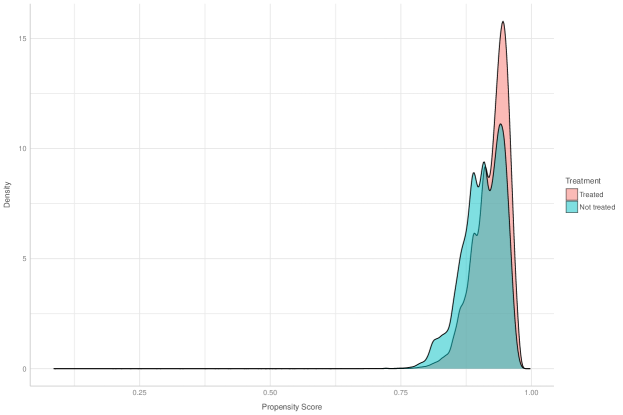
Note: Propensity scores are obtained using the Lasso with ten-fold cross validation.

Figure 2: Estimated propensity score (any treated vs. not treated)

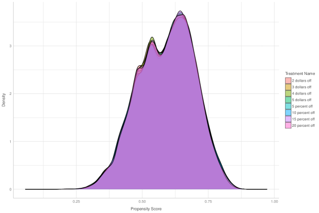
Note: Propensity scores are obtained using the Lasso with ten-fold cross validation.

Figure 3: Estimated propensity score across treated arms

We estimate a logistic regression for the propensity score of each treatment arm on our covariates using the Lasso, and we plot the distribution of the predicted propensity score in Figure 2 separately for treated and not treated individuals. We find that there is a sizable difference in the propensity scores across the two types of individuals which suggests the data might not be balanced. We then examine each treatment arm separately and estimate a logistic regression for the propensity score of each treatment arm to the no treatment arm using the Lasso and plot the predicted propensity score for only the treated individuals for each treatment arm in Figure 3. We find that there is virtually no difference in propensity scores for the treated individuals in each treatment arm. These results suggests that the randomization was correctly done across treatment arms, but may be incorrectly performed for the no treatment sample. The company has not indicated that the randomization was incorrectly implemented, but we will adjust our CATE estimations with the propensity score to account for possible mistakes or stratifications during the firm’s randomization procedure.

The firm’s goal is to maximize profits from prescribing dollar off or percentage off promotions to its customer base. The outcome variable of interest is the total profits generated from the customer $28$ days after the promotion was sent. The firm’s profit from consumer $i$ after $28$ days is defined as

$$\text{Profit after 28 days}_{i}=\text{Spending after 28 days}_{i}-\text{Promotion cost}_{i}$$ (18)

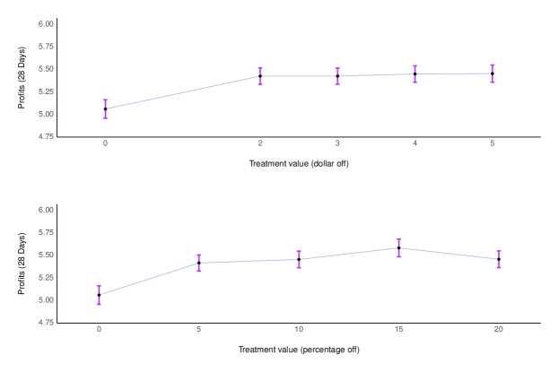
Note: The bars represent one standard deviation. Profits are sales minus promotional costs.

Figure 4: Profits by treatment

where the promotion cost depends on the promotion issued to the consumer. Figure 4 plots the profits by treatment value for dollar off and percentage off promotions. We see that in both dimensions profits earned by the firm generally increase with a higher promotion values and they roughly have a concave shape.

We then examine the results from the field experiment. The ATE estimates from the first step for the firm’s profits are presented in Table 1 which are difference in the treatment arms in Figure 4. We run a two-sided $t$-test for each treatment arm of the field experiment where we test if the null hypothesis that the ATE is zero. We report the $t$-statistics and the $p$-value for each test and find that the ATE estimates four dollar off, fifteen percentage off, and the twenty percentage off promotions are statistically significant from zero at the $\alpha=0.05$ level. Further, all of the point estimates of the ATEs are positive, which suggests the promotions have a positive effect on profits.

In terms of the notation in Section 3, profits are $\text{R}_{i}$, spending levels are $Y_{i}$, and promotion costs are $c_{d}(t_{i,d})$ where $t_{i,d}$ is treatment issued to consumer $i$ that is non-zero in dimension $d$. We only observe profits after $28$ days for each consumer and can back out the spending level after $28$ days by imposing structure on the firm’s costs. The firm’s expected returns or expected profits for individual $i$ assigned treatment $t_{i,d}$ that is non-zero in dimension $d$ is

$$E[R_{i}|\boldsymbol{x}_{i},T_{i,1}=0,\ldots,T_{i,d}=t_{i,d},\ldots,T_{i,D}=0]=E[Y_{i}|\boldsymbol{x}_{i},T_{i,1}=0,\ldots,T_{i,d}=t_{i,d},\ldots,T_{i,D}=0]-c_{d}(t_{i,d}).$$ (19)

We define the cost of the dollar amount off promotion to the firm to be the dollar amount itself. For the percentage off promotion, the firm expects the promotion cost for consumer $i$ to be the percentage off times the average promotion spending on an order by the consumer over the last $365$ days before treatment. These cost assumptions are similar to what the firm incurs in practice. We then construct the firm’s expected cost for offering consumer $i$ a percentage promotion to be

$$\text{percentage off cost to firm}_{i}=\text{percentage off promotion $\times$\text{ average past promo spend}}_{i}.$$ (20)

The cost of the promotion is then

$$c_{d}(t_{i,1}) =t_{i,1}$$ (21)

$$c_{d}(t_{i,2}) =t_{i,2}\times\text{ average past promo spend}_{i}$$ (22)

for dollar off promotion $t_{i,1}$ and for percentage off promotion $t_{i,2}$ respectively. For customers who have never received a promotion before the field experiment, their past promotion spend for an order was median imputed. Lastly, the treatment vector $(t_{i,1},t_{i,2})=(0,0)$ is the no promotion or holdout case and the firm incurs no cost by not issuing a promotion.

We also assume that the continuous CATEs, $\tau_{d}(\boldsymbol{x}_{i},t_{i,d})$, are strictly concave in the treatment value, $t_{i,d}$, to satisfy Assumption 1. The strict concavity assumption then implies that customers have diminishing sensitivities to the promotion amount so changes at higher promotion levels affect customer behavior less. By our construction of the promotion costs, they are weakly convex in $t_{i,1}$ and $t_{i,2}$ which fulfills Assumption 2.

We interpret the continuous CATEs, $\tau_{d}(\boldsymbol{x}_{i},t_{i,d})$, as a behavioral sensitivity to dollar off or percentage off treatments (Briesch, 1997). We find that even when the two yield the same expected value to the customers, the continuous treatment effect is different. In other words, customers have differing sensitivity when presented two promotions that yield the same expected monetary value. Otherwise, if consumers had the same sensitivity to the expected value of dollar off and percentage off promotions, then we would be able to collapse the two-dimensional treatment to just a one-dimensional expected value of the promotion for each customer.

4.2 Estimation procedure

To estimate the continuous CATEs, $\hat{\tau}_{d}(\boldsymbol{x}_{i},t_{i,d})$, we first implement the Causal Forest of Wager and Athey (2018) in each of the two treatment dimensions. Since we may not have a perfectly randomized experiment, we use the generalized regression forests implementation of the Causal Forest (Athey et al., 2019) that uses propensity score estimates to adjust for possible stratification between the treatments and holdout sample.

To force strict concavity of the continuous CATEs for each individual and in each dimension, we then impose a logarithmic functional form on continuous CATEs that is parameterized by $\alpha_{i,d}$ and $\beta_{i,d}$,

$$\hat{\tau}_{d}(\boldsymbol{x}_{i},t_{i,d})=\alpha_{i,d}+\beta_{i,d}\log(1+t_{i,d})+\epsilon_{i,d},$$ (23)

and a shape restriction that $\beta_{i,d}>0$. We let $\epsilon_{i,d}$ represent a vector of the approximation error. The individual continuous CATEs are parameterized by the estimates $\{\{\hat{\alpha}_{i,d},\hat{\beta}_{i,d}\}_{d=1}^{2}\}_{i=1}^{N}$, and we use these to solve for the optimal treatment levels $\{t_{i,1}^{*},t_{i,2}^{*}\}_{i=1}^{N}$ by using Equation 7. Given the optimal treatment levels and the parameterized continuous CATE estimates for each individual and dimension of treatment, we run Algorithm 1 with a choice of the number of treatments $L$ to attain the unique treatment values and their assignments. A logarithmic parameterization of the marketing treatment response to capture diminishing sensitivity has also been used in the CRM literature (Rust and Verhoef, 2005).

We bootstrap the entire procedure to produce standard errors for our estimates. In our estimation results, we focus on the implementation uncertainty of the second step, the optimal transport step, which is of main practical interest to the firm. In practice, firms treat the first step CATE estimates as given and focuses on the implementation uncertainty of the different methods in generating profits. To do so, we take the first stage treatments as the ground truth and bootstrap only the second step of our procedure. More specifically, we only bootstrap the segmentation and treatment assignment procedures from Section to 3.2 to quantify the implementation error. For the benchmark marketing segmentation procedures, we also bootstrap the segmentation and treatment assignment procedure and treat the first stage estimates of customer preferences and optimal treatment levels as the ground truth.

As a result, the comparisons of interest are (1) how well the coarse personalization solution compares to other segmentation methods and (2) how close can coarse personalization get to the fully granular personalization profits. The first comparison examines if our proposed procedure outperforms to more classical marketing segmentation procedures. The second comparison demonstrates how close in profits a firm offering a limited set of promotions can achieve compared to that of offering fully personalized and granular promotions.

4.3 Results

We provide results using a dataset of over $1.2$ million customers and use a hundred bootstrap iterations to quantify uncertainty in our estimates. The first step’s CATE estimates were estimated using the entire set of $126$ covariates and on the entire data set of $1,213,390$ individuals. The continuous CATE parameterization produced an average $R^{2}$ of $0.925$ and $0.770$ respectively for the dollar off and percentage off dimensions. We then dropped $10,011$ individuals whose $\hat{\beta}_{i,d}$ where were $10^{-6}$ or smaller since their continuous CATE estimates were not well approximated by the logarithmic functional form. We implement the honest validation procedure (Misra, 2021) to compare the continuous CATE parameterization in Equation 23 to the non-parametric estimates in a holdout set and find that our parameterization performs well. Details and the results of the validation procedure can be found in Appendix Section B.

From our parameterization of the CATEs, the individuals whose $\hat{\beta}_{i,d}$ are close to $0$ are those who are not responsive to promotions. Once accounting for the cost of the promotions, these individuals would not be given a promotion. Thus, dropping these individuals does not have an effect on incremental profits, which is our metric of interest. The second step was run on the remaining $1,203,379$ individuals and bootstrap procedure was implemented for the second step to quantify implementation uncertainty.

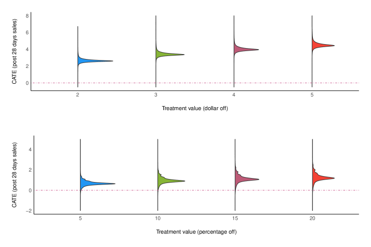
Figure 5: Continuous CATE densities for sales

Figure 5 provide the continuous CATE estimates evaluated at the randomized level of treatment in each dimension and across individuals. We see that the treatment effects generally increase as the promotion value increases in each dimension and that the treatment effect of the percentage off promotion has more variance than the dollar off promotion. On average, customers are more receptive to the dollar off promotions than to the percentage off promotion since the CATE levels are higher for the former.

In Figure 6, we plot the optimal treatment values, $\{t_{i,1}^{*},t_{i,2}^{*}\}_{i=1}^{N}$, across individuals as well as the individuals’ assigned treatment. The optimal treatment values represent the treatment values in each treatment dimension for the individuals under fully granular personalization.Table 2 provides the treatment values for the assigned treatments and their segment size. The expected incremental profits for each individual under the assigned treatment is provided on the vertical axis and a plane at zero expected profits is provided for reference. The points represent the optimal treatment values $\{t_{i,1}^{*},t_{i,2}^{*}\}_{i=1}^{N}$ across individuals and the colors represent their assignments to the unique treatments. The shape of the points represent whether the assigned treatment is a dollar off (circle) or a percentage off (triangle) promotion.

The takeaways from Figure 6 are threefold. First, across the two dimensions of treatment, the dollar and percentage off, we see explicit quantization of the assignments in each dimension. Among the six segments are assigned the dollar off promotion, we see that there is no cross contamination of segments membership across one dimension of treatment. For the percentage off promotion, the same quantization of the four segments occurs. The quantization structure results from our optimal transport setup in the coarse personalization problem and implies people who yield similar incremental profits from an assigned treatment are grouped together in a segment.

Second, we see substantial heterogeneity in individual-level expected incremental profits across the assigned individuals. Most of the generated individual incremental profits from the segments are close to zero and the profits generally increases for those with higher optimal treatment levels. The highest individual incremental profits are those given the highest percentage off promotion along with those given the highest dollar off promotion. This result suggests that those who are the most receptive to the promotions are the ones generating the most profits for the firm. There are also a handful of individuals with the lowest dollar off and percentage off promotions who have a negative individual expected incremental profit. If the firm was able to further segment, these individuals would be given no treatment or an even smaller promotional value.

Third, there is significant bunching of individuals at the upper bound in Figure 6 for the percentage off treatment which suggests we are leaving profits on the table by enforcing this upper bound. While we can expand the upper bound of allowed treatments using our parameterization of the continuous CATE estimates, we retain the upper bound at $\$5$ and $20\%$ in the optimal transport problem because this was the largest promotion in each dimension that the RCT had randomized over. In future field experiments, the firm may consider randomizing over a larger set of treatments.

Table 2 shows that most of the customers are assigned to the second, tenth, and seventh treatments and these are all dollar off promotions. We see that many of the offered treatments are tightly packed between the one to two dollar off promotion in Figure 6 which suggests that most individuals who are most receptive to the firm using dollar off promotions between one and two dollars off.

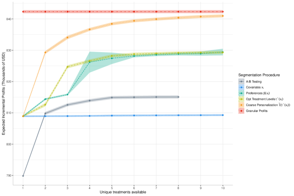
Note: The lines are the bootstrap means and the bands represent one bootstrap standard deviation. The band around the fully granular profits line reflects the sampling variation across the $100$ bootstrap iterations. The granular profits benchmark represents issuing $2,206$ unique treatments that are rounded to three significant figures. The details for the benchmark segmentation procedure can be found in Section 4.3.

Figure 7: Profit comparisons

Table 3 shows the percentage of expected incremental profits recouped by coarse personalization compared to the fully granular personalization case and Figure 7 plots the expected incremental profits across bootstrap iterations for coarse personalization. The lines represent the bootstrap means and the bands represent one bootstrap standard deviation. Fully granular personalization corresponds to issuing $2,206$ unique treatments in our scenario when rounding to three significant figures.

We find that after three unique treatments, we recoup around $99\%$ of the fully granular personalization’s expected profits and after five unique treatments, we recoup over $99.5\%$ of the fully granular personalization’s expected profits. These results suggest that the firm is able to match almost all of the fully granular personalization’s expected profits by using only a handful of unique treatments with our coarse personalization procedure.

4.3.1 Classical segmentation procedures comparison

We compare our coarse personalization estimates to traditional marketing segmentation procedures of segmenting on covariates, individual preferences, and optimal treatment levels. The comparison to classical segmentation procedures (1) sheds insight on why our coarse personalization procedure performs better by targeting profits when forming segments and (2) quantifies how much our proposed procedure outperforms the classic models. These comparisons are summarized in Figure 7.

We first consider segmenting on our covariates which contain customers’ platform behavior and RFM variables. We reduce the covariate size to $59$ covariates by retaining variables that are relevant either for predicting subsequent purchase incidence or purchase amount. Then, for this reduced set of covariates we implement $k$-means to segment the data and select the best treatment value in generating profits for each segment as the assigned treatment. This segmentation procedure represents classical ex ante segmentation since neither the outcome nor treatment variables from the data are used in forming the segments themselves after the variable reduction step.

The covariate variable reduction is done by running two Lassos where the first one is a Logit regression to predict purchase incidence and the second one predicts the amount of spending conditional on purchase incidence. Both Lasso models included all the covariates, dummies for the treatments and first order interactions between the covariates the the treatment indicators. We then select the covariates if they or their first order interaction term is given a non-zero coefficient in either regression. This procedure reduces the initial $126$ covariates to a smaller set of $59$ covariates. The $59$ RFM covariates include variables that capture customers’ past spending, tipping, delivery vs. pickup, and order cancellation behavior, promotional spending, their CBSA location, and the device they use to order.

To segment on consumer preferences, we can form segments on the treatment sensitivity of individuals and we implement $k$-means on the $\{\hat{\beta}_{i,1},\hat{\beta}_{i,2}\}_{i=1}^{N}$ estimates from our parameterization of the CATEs to form the segments. The $\hat{\beta}_{i,1},\hat{\beta}_{i,2}$ parameters capture the sensitivity of the individuals to the dollar and percentage off promotions which in turn are proxies for the individuals’ price sensitivity. The segmentation procedure is run by implementing $k$-means on the two parameters across the individuals and then finding the profit maximizing treatment for each segment.

Lastly, we can cluster on the optimal treatment levels across individuals themselves and we implement $k$-means on $\{t_{i,1}^{*},t_{i,2}^{*}\}_{i=1}^{N}$. The optimal treatment levels are the individually optimal promotion values for each individual under fully granular targeting. Forming segments using $k$-means in this setting lead to individuals who have similar individually optimal promotions to be put in the same segment. This means that individuals with the same dollar off and percentage off individually optimal treatments will be assigned to the same segment. After the segments are made, we find the optimal treatment level for each segment by choosing the level and dimension of treatment that maximizes profits.

Figure 7 and Table 3 also show the expected incremental profits arising from separately forming segments based on covariates, preferences, and optimal treatment levels and then finding the optimal treatment for each segment. For our implementation of our approach using Algorithm 1 and the other benchmarks using $k$-means, we use five different sets of starting points for each segmentation and choose the one that produced the highest expected profits.

We find that our coarse personalization methodology (“personalize then discretize”) significantly outperforms the other standard segmentation methods (“discretize then personalize”) that are used in the classical marketing literature. With our framework, coarse personalization generates the maximum expected profits possible given the limitation on the number of unique treatments available to the firm.

Segmenting on covariates does not appear to help the firm in maximizing profits because the segments based on consumer characteristics do not necessarily correspond to the optimal segments for maximizing profits. Segmenting on consumer preferences and optimal treatment levels does better than segmenting on covariates. These results corroborate the results found in the traditional marketing segmentation (Gupta and Chintagunta, 1994; Rossi et al., 1996) and CRM literature (Rust and Verhoef, 2005) where they find forming segments on demographic and RFM covariates do not produce the most profit maximizing segments and segmenting on consumer preferences performs better in generating profits.

Since optimal treatment levels are constructed from the consumer preferences and the cost function faced by the firm, the segmenting on preferences and optimal treatment levels embed similar information and thus should perform similarly. Segmenting on preferences is noisier than segmenting on optimal treatment levels because the latter is more directly related to the profit maximization problem and accounts for treatment costs. The difference in profits between segmenting on optimal treatment levels and our coarse personalization procedure arises because coarse personalization uses the correct distance metric of expected profits for segmentation. This specific difference in exemplified in Figure 6 from the quantization of the segments in treatment dimension. For each individual, the nearest treatment on Figure 6 is not necessarily assigned because the distance metric used for segmentation is in expected profits (Equation 12) and is not Euclidean distance in the optimal treatment values. As a result, the constructed segments from coarse personalization will outperform those constructed from using the optimal treatment level when firm’s goal is to maximize expected profits.

4.3.2 A/B testing with discrete treatments comparison

We provide two comparisons to standard A/B testing when treating the eight treatments arms ($2,3,4,5$ dollar off promotions, $5,10,15,20$ percentage off promotions) from the field experiment as separate discrete treatments. In both cases, the firm ignores the continuous nature of the dollar and percentage off promotions and only looks at the treatments that were implemented in the experiment.

We first examine the optimal blanket treatment to demonstrate the profit differences between the firm’s current blanket promotion of ten percent off and an optimized blanket treatment where (1) the firm only uses the experiment’s discrete treatments and (2) the firm leverages the continuity of the treatments. This comparison demonstrates how much money the firm leaves on the table by not optimizing the blanket treatment itself.

We then examine if the firm decided to use offer up to the eight discrete treatment from the field experiments as the possible offered treatments which then forms up to eight different segments. We compare the profits from this benchmark to our coarse personalization solution to demonstrate the value added from our procedure over segmenting based on the A/B testing results.

If the firm chose the best treatment arm from the RCT to blanket target, the firm would offer the two dollar off promotion and attain expected profits of $789,868$ dollars which is $93.8\%$ of the fully granular benchmark. In the continuous treatments case, the firm would choose $1.70$ dollars off blanketed to the whole population. This blanket treatment generated $808,920$ dollars in expected profit which recovers $96\%$ of the fully granular benchmark as seen in Table 3.

In contrast, the firm’s most recently blanketed promotion, a $10\%$ off coupon, would yield only $330,278$ in profits which is $39.21\%$ of the fully granular benchmark. Thus, for choosing a blanket treatment, optimizing the treatment itself does a sizable amount of work of getting close to the fully granular personalization profits. Allowing for continuous treatments rather than discrete treatments provides further expected profit gain for the firm.

We now consider the case where the firm offers up to all eight treatments used in the experiment and reports it as the A/B testing benchmark in Figure 7. The A/B testing benchmark with one offered treatment is just the optimized blanket treatment among the discrete treatment arms at two dollars off.

We construct this A/B testing benchmark using the eight discrete treatments as possible treatments to assign. For example, for issuing three unique treatments, we combinatorially search through the $\binom{8}{3}=56$ possible combinations of treatments. For each combination of offered treatments, we form the segments by first computing the profits for assigning each individual to each offered treatment and then assigning the treatment that produces the highest expected profits to that individual. We sum the expected profits across the offered treatments and their assignments to get the total expected profits for that specific combination of offered treatments. Lastly, we choose the combination of the offered treatments that produces the highest profits as the A/B testing benchmark value.

From Figure 7, we find that the A/B testing benchmark does better than segmenting on covariates, but performs significantly worse than segmenting on consumers’ preferences, optimal treatment level, and our coarse personalization procedure. The difference between the A/B testing benchmark from our coarse personalization solution demonstrates the profit gain from allowing the treatments to be continuous which then allows optimization over which treatment values to offer.

4.3.3 Rounded treatment levels

Since decimal level treatment values may not be applicable for various settings, we further examine the coarse personalization problem with rounded treatments. By a priori discretizing the space of possible treatments, we can no longer guarantee that the solution to the Monge-Kantorovich Problem in Equation 8 is unique. As a result, we empirically examine two different rounding procedures. The first is ex ante rounding, where we only allow Algorithm 1 to consider when integer treatments when updating. The second is ex post rounding, where we round the treatment levels after running Algorithm 1. In the latter case, because two unique treatments might be rounded to the same value, the effective number of unique treatments may be reduced by the rounding procedure.

Table 4 demonstrates the percentage of expected incremental profits with by coarse personalization with the two integer rounding procedures. Fully granular personalization with integer treatments only allows for $26$ unique treatments in this setting. Comparing Table 3 to Table 4, we see that we leave some profits on the table with both rounding procedures. The fully granular personalization profits with integer treatments lies between that of offering one and two unrounded treatments. From Table 4, we see that with ex ante rounding we can recover almost all of the fully granular rounded treatment profits after ten unique integer treatments. With ex post rounding, we see that the effective number of treatments is often smaller than the number of unique treatments before rounding. Further, the best performing set of ex post rounded treatments is similar to the set of ex ante rounded treatments. The differences across profits with the same effective number of treatments arises because the ex post rounding itself is ad hoc and not necessarily profit maximizing. In contrast, rounding ex ante in each step of Algorithm 1 ensures that constructed segments and their treatment levels are geared towards profit maximization. These results suggest that even though with rounded treatments we may not get an unique optimal solution, Algorithm 1 still does well with ex ante rounding to form segments that are assigned integer treatments in solving the coarse personalization problem.

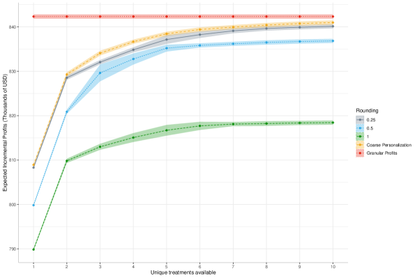
Note: The lines are the bootstrap means and the bands represent one bootstrap standard deviation. The band around the fully granular profits line reflects the sampling variation across the $100$ bootstrap iterations. The granular profits benchmark represents issuing $2,206$ unique treatments that are rounded to three significant figures.

Figure 8: Profit comparisons for coarse personalization with ex ante rounded treatments

Figure 8 demonstrate the performance of Algorithm 1 with ex ante rounding and provides the profit comparisons for the coarse personalization solution with different ex ante rounded treatments at the $0.25$, $0.5$, and $1$ (integer rounding) levels. The algorithm still performs well with the ex ante rounding because we see that profits overall increase with more granular targeting. While we almost fully recover the unrounded coarse personalization results by rounding at the $0.25$ level, in practice that level of rounding is often too granular for the firm. Rounding at $0.5$ or at integer values leads statistically significant lower profits than rounding at $0.25$, but the firm is still able to almost recover all of the fully granular profits while still only offering only five unique treatments in either case. The optimal rounding level of the treatments will ultimately depend on the firm’s application and how much it is willing to leave profit on the table for more rounded treatments.

5 Surplus analysis

We can use our coarse personalization framework to examine the effects of better personalization and targeting on consumer surplus and producer surplus. While it is clear that producer surplus will monotonically increase as the firm can better personalize, its effect is not clear on consumer surplus. Some consumer receive higher or lower consumer surplus by being assigned a treatment that is above or below their assigned treatment under fully granular personalization. Due to the uncertain effect on consumer surplus, the total surplus produced for an individual may be higher or lower than that of under the fully granular personalization scenario. This section provides an empirical quantification of this effect in our promotions management setting.

To close our model for a surplus calculation, we need to impose assumptions on the individual valuation of the treatments $v_{i}(t_{i,d})$. We assume that the consumer values the dollar off coupon at face value ($v_{i}(t_{i,1})=t_{i,1}$) and values the percentage off coupon at the percentage off rate times the average past promotion spend for an order ($v_{i}(t_{i,2})=t_{i,2}\times\text{ average past promo spend}_{i}$). These valuations match the cost of issuing the promotion for the firm and we can treat the promotion as a transfer from the firm to the consumer that further stimulates demand from the consumer. Armed with the firm’s program (Equation 7) and the assumption on consumer valuations, we can compute the total surplus (Equation 29) and estimate the change in surplus for each individual under different levels of coarse personalization compared to the fully granular personalization benchmark. We defer the complete surplus calculation procedure to Appendix Section C.

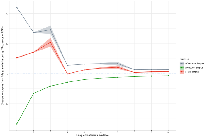
Note: The lines are the bootstrap means and the bands represent one bootstrap standard deviation.

Figure 9: Surplus decomposition across treatments

From Figure 9 and Table 5, we observe that there is a non-monotonic relationship of consumer surplus to the number of unique treatments available. The lines in Figure 9 represent the bootstrap means and the bands represent one bootstrap standard deviation for the change in welfare surplus from that of the fully granular benchmark. The consumer surplus is highest when there is one unique treatment ($L=1$) and decreases as the firm can use more treatments. Further, the consumer surplus drops significantly after four unique treatments and then drops sizably again after eight unique treatments. The non-monotonic changes in consumer surplus arise from the trade-off between the firm assigning treatments to individuals that are different from their individual optimal treatment level and that the firm chooses the assignment of individuals so the individual often cannot benefit too much from the assignment at the expense of the firm.

Table 6 provides the surplus decomposition of the change total surplus into the change in producer surplus and consumer surplus for when the firm issues ten unique treatments ($L=10$). Each row in the table represents the respective unique treatment in Table 2. We see that compared to the fully granular personalization benchmark, producer surplus is always reduced under coarse personalization. Further, we see that the changes in consumer surplus contributes most to the changes in total surplus from Table 5.

From Tables 2 and 6, we see that most of the customers are assigned to three unique treatments. In turn, three unique treatments captures a sizable portion of the expected profit gain from coarse personalization. As a result, when the firm is able to assign four unique treatments, it is able assign all the individuals who did not fit the three unique treatments and the firm lost profits on into the fourth treatment. Since these are the consumers who are likely benefiting from the constraint in the three unique treatment case, this result explains the significant drop in consumer surplus in Figure 9 from going from three to four unique treatments.

Our empirical findings corroborate the non-monotonic relationship of personalization and consumer surplus in Dube and Misra (2022). We further see that from Figure 9 and Table 5, the gain in consumer surplus for being assigned a suboptimal treatment generally dwarfs the loss of producer surplus. As a result, we see that total surplus increases with coarser targeting. These findings lie opposite to the the theoretical equilibrium results in Bergemann and Bonatti (2011), which finds that total surplus increases as advertisers are better able to personalize and meet the needs of the consumers. Even though our surplus calculation uses an simplified model of the consumer valuation of promotions, we still see that the results from better personalization can be non-monotonic and will depend on the consumers’ valuations. Future research should utilize panel data for a more rigorous surplus calculation to flesh out the non-monotonic relationship between personalization and consumer surplus as well as examine the long-term effect of personalized promotions on societal surplus.

Lastly, our surplus formulation offers a convenient rule to choose the number of unique treatments to offer from a societal perspective. From Figure 9 we see that offering three unique treatments maximizes the total societal surplus while allowing the firm to recover $99\%$ of fully granular profits. Since the change in total surplus is positive, more deadweight loss is generated in the fully granular case than when coarse personalizing by offering only three unique treatments. Thus, in preempting possible fairness or antitrust concerns, the firm may be inclined to offer only three unique treatments and leave $1\%$ of the fully granular profits left on the table.

6 Discussion

Outside of the our empirical application where we revisited the traditional segmentation procedures for promotions management, we can also adapt our coarse personalization procedure to a variety of different marketing applications. In this section, we provide a handful of classical marketing scenarios where our framework can be used. In some of the examples, the assumption that the treatment vector is non-zero in one treatment dimension can be relaxed and interactions across treatments can be allowed. However, in practice, this requires much more data to be used in the first step in order to estimate the interactions.

In the context of salesforce compensation, managers need to decide which geographic blocks of individuals to assign to which salespeople, how long much time the salespeople should spend on visit, and whether the visits should be in person or over the phone (Misra, 2019). The dimensions of treatment in this example are the time spent and the type of visit. Further, often only a handful of geographic blocks are assigned to each salesperson (Zoltners and Sinha, 1983). Managers can use the coarse personalization procedure to design the optimal geographic blocks as well as visits types for their salespeople to maximize expected sales profits.

In the “contract externality” framework of Daljord et al. (2016), salesforce managers choose a homogeneous contract commission rate and the assignment of heterogeneously effective salespeople to that contract. “Contract externalities” arise because the choice of the salespeoples’ assignment will affect the optimal contract commission rate. The firm’s manager then chooses the treatment level, the homogeneous commission rate, and the composition of the salespeople who are assigned to each treatment. Daljord et al. (2016) focus on a one-dimensional contract rate while our framework allows for a finite dimensional number of contract components.

We can also apply our methodology to advertising design. For example, Bertrand et al. (2010) find that for small loans, altering advertising features, such as the advertisement’s photo and content, has a significant effect on increasing a loan’s demand that is comparable to changing the loan’s interest rate. If their firm decides to choose a handful of advertisements to coarsely personalize and send out, then the findings from Bertrand et al. (2010) provide the first step’s results in our procedure. We would then account for how many different advertisements the firm is willing to send out and determine which optimal advertisements to offer using our second step.

Our framework can also be used to guide pricing decisions. Chandar et al. (2019) find that across 40 million Uber rides, riders have heterogeneous preferences over private tipping behavior. If firm managers aim to maximize tip and overall spending from customers but cannot fully personalize due to fairness concerns, they can assign different geographic blocks of riders going to the same location the same baseline price and the suggested default tip rate. By coarsely personalizing, the managers can both increase profits by personalizing and address fairness concerns – two people in the same area searching for a ride to the nearest airport will face the same price.

Lastly, coarse personalization can be interpreted as a more regularized version of the fully granularly personalized case. Heterogeneous treatment effect estimates are known to be noisy (Hitsch et al., 2023; Wager and Athey, 2018), and by coarsely assigning blocks or segments of customers that are given the same treatment, firms are able to explicitly choose the level of regularization to incorporate when using the heterogeneous treatment effects. At one extreme, full regularization implies everyone receives the same treatment and at the other, fully granular personalization is implemented and everyone gets her own fully personalized treatment. The coarse personalization framework enables a firm’s manager navigate between two extremes while ensuring the profit maximizing groups and treatments are formed at each level of regularization.

7 Conclusion

Advances in heterogeneous treatment effect estimators have allowed for granular incrementality-based targeting and personalization in a myriad of social science applications. While these methods enable individual-level personalization and fully granular segmentation, firms or institutions in practice often only offer a handful of unique treatments due to menu costs, fairness constraints, antitrust considerations, etc. We denote this practical problem as the coarse personalization problem in which firms need to choose both the unique treatments to offer and the assignment of individuals to the selected treatments. We provide a link of what is available theoretically to what is done in practice with our solution to the coarse personalization problem.

In this paper, we utilize methods from the optimal transport literature to solve the coarse personalization problem. We propose a two-step approach where the first step estimates the conditional average treatment effects and the second step solves the constrained assignment problem. The first step itself is already used in the literature and provides the fully granular personalization solution. The second step is a novel application of the optimal transport and maps the distribution of conditional average treatment effects to a set of discrete treatments. Our solution revisits the traditional marketing framework with modern machinery and we advocate for a “personalize then discretize” approach that forms segments and chooses their assigned treatments simultaneously, instead of the traditional “discretize then personalize” approach that forms segments and their assigned treatments sequentially.

There are practical implications of the methodological results from this paper. We provide an empirical application for promotions management using field experiment data from a large food delivery platform. We find that after assigning five unique treatments, the company is able to recoup over $99.5\%$ of its expected profits from fully granular personalization. Our approach outperforms traditional marketing procedures that segments on covariates or preferences. Further, our proposed algorithmic solution is both scalable and easy to implement. These results have direct managerial implications as we offer a practical way for firms and marketers to optimally coarsely personalize their offerings. Future research can examine the effects of competition on firms implementing our coarse personalization procedure.

Our methodology can be generally used for constrained assignment problems in other fields. Using drug trial data, we can find the best drug and dosage level combinations for pharmaceutical companies to provide. Drug companies can then coarsely personalize medicine for their clientele. The optimal transport solution itself can be adapted to solve for optimal teacher assignments with peer effects or for optimally allocating workers to projects and collaborative tasks.

We view our paper as a bridge linking optimal transport theory to practical problems in the social sciences. Optimal transport methods have been utilized in economics for many applications that are surveyed in Galichon (2016). In computer science, optimal transport has been used for a variety of problems ranging from training high-dimensional GANs to computer vision (Peyré and Cuturi, 2019). This paper utilizes optimal transport as a novel way to solve a practical problem and future research in applying optimal transport to other problems in social science is already underway.

Figures

Figure 1: Adapted Lloyd’s Algorithm ($D=2$)

Note: This figure provides a stylized visualization of Algorithm 1 with two-dimensional treatments $(D=2)$ and three treatments to be assigned/segments ($L=3)$. The horizontal axis represents the treatment values for the first dimension and the vertical axis represents that of the second dimension. The points on the axis represent the offered treatment values $\boldsymbol{t}_{l}$, the interior points represent the individual optimal treatment values $(t_{i,d=1},t_{i,d=2})$, the lines represent the Voronoi Cells’ boundaries, and the square points represent the Barycenters of each cell. A more detailed outline of the algorithm is provided in Subsection 3.3.1.

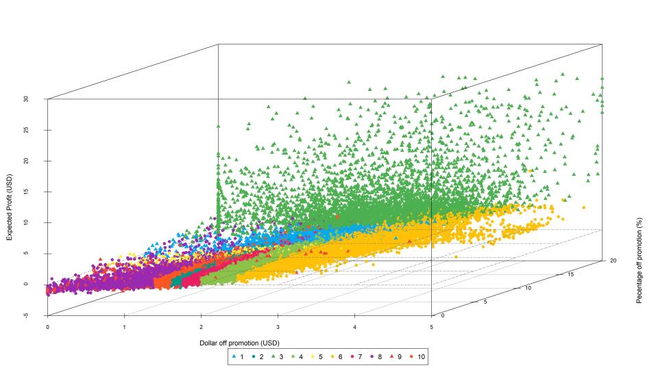
Note: The optimal (granular) treatment assignment for each person is plotted for the dollar off and the percentage off promotions. The colors represent each individual’s assigned treatments. The triangular points indicate those individuals are assigned a percentage off treatment and the circular points represents the those who are assigned the dollar off promotion. The assigned treatments’ values can be found in Table 2. The incremental expected profits generated from the treatment assignments for each individual is plotted on the vertical axis. A horizontal plane plotted at zero expected profits is provided for reference.

Figure 6: Treatment assignments ($L=10$ treatments)

Tables

Table 1: Field experiment average treatment effects on profits

Treatment value	ATE	SE	$t$-stat	$p$-value
Dollar off
2	0.034	0.046	0.730	0.465
3	0.061	0.046	1.326	0.185
4	0.122	0.047	2.605	0.009
5	0.085	0.049	1.722	0.085
Percentage off
5	0.056	0.045	1.225	0.220
10	0.078	0.047	1.659	0.097
15	0.153	0.047	3.220	0.001
20	0.096	0.045	2.101	0.036

Note: The average treatment effects (ATEs) estimated from the Causal Forest comparing each treatment arm to the holdout set of issuing no promotion. The reported $t$-statistic and the $p$-value are for a two-sided $t$-test against the null hypothesis that the ATE for each promotion is 0.

Table 2: Treatment assignments ($L=10$)

Treatment ($l$)	Dimension ($d$)	Value ($t_{i,d}$)	$N$
1	Percentage	12.45	7,090
2	Dollar	1.67	556,544
3	Percentage	20.00	7,375
4	Dollar	2.15	54,253
5	Percentage	8.42	12,816
6	Dollar	2.79	15,532
7	Dollar	1.83	214,631
8	Dollar	1.24	30,425
9	Percentage	5.17	9,234
10	Dollar	1.54	295,479

Note: The table lists the ten treatments assignments in Figure 6.

Table 3: Expected incremental profits by segmentation method

	Profits by segmentation method ($)
Number of treatments ($L$)	Covariates	Preferences	Optimal treatment levels	Coarse personalization
1	808,920	808,920	808,920	808,920
2	808,940	814,377	812,609	829,300
3	808,969	815,851	824,710	834,085
4	809,021	826,215	826,581	836,669
5	809,114	827,432	828,205	838,450
6	809,156	828,159	828,766	839,417
7	809,190	828,568	828,970	839,954
8	809,226	828,817	829,159	840,412
9	809,247	828,929	829,243	840,761
10	809,277	829,429	829,315	840,985

(a) Profit by segmentation method and number of treatments

Benchmark	Profits ($)
Firm’s blanket promotion (10% off)	330,278
A/B testing blanket ($2)	789,868
Fully granular targeting	842,366

(b) Benchmark profit comparisons

Note: The firm’s recent blanket promotion was a $10\%$ off blanket promotion. The A/B tested optimal blanket promotion is a $\$2$ off promotion. When $L=1$, the optimal blanketed promotion is a $\$1.70$ off promotion for all the segmentation methods. Fully granular personalization would use 2,206 unique promotions when rounding to three significant figures.

Table 4: Expected incremental profits by the number of treatments (rounded integer treatments)

	Ex ante Rounding		Ex post Rounding
Number of treatments ($L$)	Profits ($\$$)	Percent to granular $(\%)$	Profits ($\$$)	Percent to granular $(\%)$	Effective treatments
1	789,868	96.50	789,868	96.50	1
2	809,849	98.95	809,789	98.94	2
3	812,964	99.33	809,830	98.94	2
4	814,335	99.49	812,825	99.31	3
5	816,677	99.78	812,788	99.30	3
6	817,753	99.91	815,261	99.61	5
7	818,116	99.96	817,299	99.86	5
8	818,265	99.97	817,801	99.92	6
9	818,394	99.99	817,516	99.88	6
10	818,471	100.0	815,917	99.69	6
Fully granular (26)	818,481	–	818,481	–	–

Note: Fully granular targeting with rounded integer treatments involves issuing $26$ unique treatments.

Table 5: Surplus decomposition across treatments

Number of treatments ($L$)	$\Delta TS$	$\Delta TS_{i}>0$ (%)	$\Delta CS$	$\Delta CS_{i}>0$ (%)	$\Delta PS$	$\Delta PS_{i}>0$ (%)
1	10,613	64.16	44,029	64.54	-33,416	0
2	14,348	62.38	27,387	62.38	-13,040	0
3	21,248	50.29	29,483	50.29	-8,234	0
4	-123	49.71	5,546	49.71	-5,668	0
5	2,469	46.05	6,358	46.05	-3,889	0
6	3,807	51.16	6,724	51.17	-2,917	0
7	4,622	49.32	7,002	49.32	-2,380	0
8	737	49.18	2,664	49.18	-1,927	0
9	1,236	50.42	2,813	50.42	-1,577	0
10	1,543	49.98	2,883	49.98	-1,340	0

Note: $\Delta TS,\Delta CS,$ and $\Delta PS$ respectively represent the total change in total surplus, consumer surplus, and producer surplus to the fully granular personalization benchmark across individuals. $\Delta TS_{i}>0$ represents the percentage of individuals who have a positive change in total surplus to the fully granular benchmark and the other two columns ($\Delta CS_{i}>0$ and $\Delta PS_{i}>0$) are likewise defined.

Table 6: Surplus decomposition across individuals ($L=10$)

Treatment ($l$)	Average $\Delta TS_{i}$	$\Delta TS_{i}>0$ (%)	Average $\Delta CS_{i}$	$\Delta CS_{i}>0$ (%)	Average $\Delta PS_{i}$	$\Delta PS_{i}>0$ (%)	$N$
1	-57.70	56	-15.65	56	-42.04	0	7,090
2	138.73	53	299.50	53	-160.77	0	556,544
3	136.14	25	152.81	25	-16.67	0	7,375
4	22.33	58	164.97	58	-142.64	0	54,253
5	-59.35	51	-7.84	51	-51.51	0	12,816
6	-170.45	64	78.62	64	-249.07	0	15,532
7	176.26	58	332.54	58	-156.27	0	214,631
8	-8.92	33	312.48	33	-321.41	0	30,425
9	-253.45	35	-122.20	36	-131.25	0	9,234
10	133.11	40	300.28	40	-167.17	0	295,479

Note: $\Delta TS_{i},\Delta CS_{i},$ and $\Delta PS_{i}$ respectively represent the change in total surplus, consumer surplus, and producer surplus to the fully granular personalization benchmark for individual $i$. $\Delta TS_{i}>0$ represents the percentage of individuals assigned that treatment who have a positive change in total surplus to the fully granular benchmark and the other two columns ($\Delta CS_{i}>0$ and $\Delta PS_{i}>0$) are likewise defined.

Appendix

Appendix A Mathematics of Coarse Personalization

We provide a mathematical overview of our setup of the coarse personalization problem in Section 3 which incorporates an overview of the optimal transport framework that underlies our solution. We supply a canonical example used in the optimal transport literature to introduce the optimal transport framework and then link it to our promotions management setting from our empirical application. We direct readers to Galichon (2016), Santambrogio (2015), andVillani (2009) for a more formal introduction to optimal transport.

In essence, optimal transport is the study of moving mass from from one distribution to another while minimizing a established cost function. These two distributions can be continuous or discrete and solution to the optimal transport problem provides an optimal transport plan that describes how the mass is moved. The optimal transport plan pushes forward the mass from one distribution to the other

To provide a concrete example, we first consider the canonical example of physically moving earth. This optimal transport problem literally examines how to optimally move ore from the mine to the factory for processing. The optimal transport plan then details both how much ore is being moved from each factory and where the ore is being sent. An optimal transport mapping is a subset of possible optimal transport plans where all the mass from one mine will be sent to a factory. In other words, under the mapping, the mines cannot split mass by sending half of their ore into one factory and the other half to another factory. More generally, the optimal transport plan is probabilistic assignment of mines to factories while the optimal transport plan is a deterministic assignment of mines to factories.

While in practice, the number mines and factories are discrete, in theory the results for the earth moving example can be extended to continuous distributions of mines and/or factories. In the continuous to continuous case, the optimal transport plan will maps parts of the cumulative distribution functions of the two distributions to one another.

In our promotions management setting, we replace mines with a continuous distribution of the heterogeneous treatment effects across the individuals in our data that we had estimated from the field experiment (Section 3.1). We replace factories with the discrete number of treatments the firm decides to assign and we have a continuous-discrete or a semidiscrete optimal transport problem. Since the treatments, or promotions, can be dollar off or percentage off, we have a two-dimensional continuous distribution to map the discrete treatments to.

Our coarse personalization problem in Equation 9 has two nested problems. The inner problem is the optimal transport problem where the segment assignments are formed. The outer problem chooses the treatment levels to assign as well as the size of each segment.

We focus on the inner problem or the Monge-Kantorovich problem (Equation 8) that is the optimal transport problem for this section. We let the $P$ be the distribution of heterogeneous treatment effects and $\tilde{t}=\{\tilde{\boldsymbol{t}}_{1},\tilde{\boldsymbol{t}}_{2},\ldots,\tilde{\boldsymbol{t}}_{L}\}$ be sample of the $L$ points or treatments that need to assign. These treatments are distributed by $Q^{\tilde{t},q}$ where each treatment has probability mass $q_{l}$ for each treatment $\tilde{\boldsymbol{t}}_{l}$ such that $\sum_{l=1}^{L}q_{l}=1$. Both distributions are over the space of real numbers.

In this setup, we want to map the continuous distribution heterogeneous treatment effects to the discrete distribution of $L$ treatments to be assigned. The probability mass $q_{l}$ for treatment $\tilde{\boldsymbol{t}}_{l}$ represents the portion of the total number of individuals assigned to treatment $l\in L$. In the marketing literature, we let the $L$ different treatments form $L$ different segments where each segment is assigned treatment $\boldsymbol{t}_{l}$ and $q_{l}$ describes the size of segment $l\in L$. The distribution of heterogeneous treatment effects is then across the individuals in the field experiment.

We define the notion of a coupling, which determines which individuals with a certain level of the heterogeneous treatment effect will be assigned to one of the treatment. These couplings form the optimal transport plan between two distributions and inform how the mass is moved across the two. More formally, following Galichon (2016), we let $\mathcal{X}\sim P$ and $\mathcal{Y}\sim Q^{\tilde{t},q}$. Then the set of couplings over the probability distributions $P$ and $Q^{\tilde{t},q}$ is the set of probability distributions $\mathcal{X}\times\mathcal{Y}$ with first and second marginal distributions as $P$ and $Q^{\tilde{t},q}$. The set of couplings is defined as $\mathcal{M}(P,Q^{\tilde{t},q})$. Thus, a probability measure $\pi$ over $\mathcal{X}\times\mathcal{Y}$ is in $\mathcal{M}(P,Q^{\tilde{t},q})$ if and only if $\pi(A\times\mathcal{Y})=P(A)$ and $\pi(\mathcal{X}\times B)=Q^{\tilde{t},q}(B)$ for every subset $A\subseteq\mathcal{X}$ and $B\subseteq\mathcal{Y}$. Then a random pair $(X,Y)\sim\pi$ where $\pi\in\mathcal{M}(P,Q^{\tilde{t},q})$ is a coupling of $P$ and $Q^{\tilde{t},q}$.

For a coupling $(X,Y)$ where $Y=T(X)$ is a deterministic function of $X$, the transport plan $T(\cdot)$ will be a transport map. This is also known as pure assignment or a Monge coupling/mapping. The map implies that all for an individual with specific values of $x\in X$, she will be assigned to only one treatment (or segment) and not probabilistic assigned to many treatments.

The Monge problem then finds the optimal pure assignments to minimize a cost function,

$$\min_{T(\cdot)} \ E_{P}[C(X,T(X))]$$ (24)

s.t. $$\ T\#P=Q^{\tilde{t},q}$$ (25)

where $C(X,Y)$ is the cost function and $T\#P$ is the push-forward of probability $P$ by map $T$. $T\#P=Q^{\tilde{t},q}$ is defined such that that if $X\sim P$, then $T(X)\sim Q^{\tilde{t},q}$. The cost function specifies the cost of transporting mass from $X$ to $Y$ and in our setting it represents the lost profits due to coarse personalization instead of fully granular personalization (Equation 12).

In general, the Monge problem may not have a solution so we take the relaxation of the Monge problem, which is the Monge-Kantorovich problem. The Monge-Kantorovich problem solves for an optimal transport plan,

$$\min_{\pi\in\mathcal{M}(P,Q^{\tilde{t},q})}E_{\pi}[C(X,Y)]$$ (26)

where the couplings $\pi$ are optimized over instead of the pure assignments $T(\cdot)$ from the Monge problem. The relaxation to the Monge problem implies that the optimal couplings may require some of the individuals to be probabilistically assigned to different treatments, or split mass, between different segments. In the traditional marketing literature, the probabilistic segmentation parallels the approach espoused in Kamakura and Russell (1989).

Under some conditions, the Monge-Kantorovich problem produces the same solution as the Monge problem and the optimal transport plan is the same as the optimal transport map. In our setting, this implies that segment assignments of individuals to treatments are deterministic. In our semidiscrete optimal transport problem, we show in Proposition 3 that the coarse targeting problem is strictly convex in the treatment values. The strict convexity implies that a solution the optimal transport problem will exist and that we will have a pure assignment of individuals to segments. The former is provided as from a results in Theorem 2.2 in Galichon (2016). The latter is a result from convex analysis as Rademacher’s Theorem implies the set of non-differentiable points will be Lebesgue measure zero and can be ignored under a continuous $P$. Since the non-differentiable points are the individuals who are probabilistically assigned many segments, this results implies that we will attain a deterministic mapping of individuals to their assigned segments and each individual will only be mapped to one segment.

Appendix B Honest validation for CATE estimation

We use the honest validation procedure introduced in Misra (2021) to provide an out-of-sample performance evaluation for the parametric form for the continuous CATEs (Equation 23) to the non-parametric CATE estimates for each treatment arm. The honest validation procedure leverages the fact that the treatment arms are discrete while the treatments are themselves continuous to provide a comparison of the parameterized estimate to the non-parameteric estimates in a holdout set. We detail the procedure and describe the evaluation in the remainder of this section.

The honest validation procedure is implemented in four steps. First, we use the Causal Forest estimates for each of the eight treatment arms ($2,3,4,5$ dollars off and $5,10,15,20$ percentage off).

Second, for each individual, we hold out her actual treatment assignment and use the predicted CATEs to estimate her parameterized CATE function (Equation 23). The estimation is only done in the dimension of treatment that she was assigned. For example, if she was was assigned to a two dollar off promotion in the field experiment, we would use her predicted CATEs for the other dollar off treatment arms ($0,3,4,5$ dollars off) to estimate the her parameterized CATE function. The two dollar off promotion is held out in this step and consists of the hold-out set for the parameterized estimate.

Third, we use the parameterized CATE function to predict the CATE estimate for the held out treatment. In our running example, we would predict her CATE using the parameterized CATE function for two dollars off. The two dollar off promotion was her assigned treatment from the field experiment so we have the non-parameteric Causal Forest estimate for her at that treatment.

Lastly, we compare the predicted CATE in the held out treatment to the non-parameteric Causal Forest estimate for the individual. In our running example, we would compare the non-parametric estimate of the individual’s CATE at two dollars off to her predicted CATE estimate at two dollars off from the parameterized CATE function.

If we treat the non-parametric estimate as the “ground truth”, then this honest validation procedure will inform us how close our chosen parameterization of the CATE function is to the non-parametric ground truth. We perform this procedure separately for each dimension of treatment — dollar off and percentage off promotions.

Figure 10 plots the parametric estimates against the non-parametric estimate for each individual. The horizontal axis represents the parametric estimates in the hold out set and the vertical axis represents the non-parametric estimate. The shapes and colors of the points represent the assigned treatment arm in the field experiment. We see that most of the points line are scattered around the $45$ degree line which suggests the two types of estimates overlap. Further, the correlation between the parametric estimate in the hold-out sample to the non-parametric estimate is $0.821$ for the dollar off and $0.604$ for the percentage off promotions. These results suggest that the parameterized CATEs perform well in the hold out set.

We see generally that the non-parametric estimates are noiser than the parametric estimates as there is more dispersion on the vertical axis in Figure 10. The parametric form imposes more structure on the CATEs which reduces the variance of the estimates. The variance of the points are higher for the percentage off promotions for both the parametric and non-parametric estimates which plays a role in why the parameterization fits the response to a dollar off promotion better than that of a percentage off promotion.

Appendix C Surplus calculation details

Bergemann and Bonatti (2011) find that as firms can better granularly personalize, they attain higher levels of producer surplus and societal total surplus generally increases in equilibrium. With our coarse personalization framework, we are able to empirically examine the theoretical results from Bergemann and Bonatti (2011). Since the firm can only choose $L$ unique treatments to assign, individuals can be assigned a treatment that is either above or below their optimal level or even in a different treatment dimension. Compared to the granular case, the consumer surplus can increase or decrease if they receive a higher or lower than optimal treatment level under our coarse personalization procedure. In contrast, the producer surplus will always diminish when the firm more coarsely targets by the optimality principle of fully granular personalization. Due to the ambiguous effect on consumer surplus, the total surplus generated for each individual $i$ can either increase or decrease compared to the fully granular case.

Intuitively, we expect that some individuals benefit from coarse personalization because they may receive a treatment that is better for them than what they would get in the fully granular personalization case. The distortion in the firm’s ability to perfectly granularly personalize creates this benefit to individuals. In determining the optimal assignments and the optimal treatments to offer, the firm trades off the gains in consumer surplus from the distortion and the profits they gain from the treatments and their assignments. However, an individual consumer cannot benefit too much lest the firm would reassign her to another treatment where the gain in consumer surplus is lower or even negative. These non-monotonic changes to the individual-level consumer surplus as the targeting ability of the firm increases directly parallels to the non-monotonicity in the consumer surplus as firms are able to use more features of the data to personalize prices in Dube and Misra (2022). Total surplus can increase or decrease with coarse personalization depending on the changes in consumer surplus relative to the producer surplus. If the consumer surplus gain from coarse personalization dwarfs the loss in producer surplus, then total surplus may increase with coarse personalization.

We formulate a simple surplus analysis to empirically examine the results from Bergemann and Bonatti (2011) and Dube and Misra (2022) in our framework. Without loss of generality, at the fully granular personalization benchmark, individual $i$ is offered treatment value $t_{i,d}^{*}$ that is non-zero in dimension $d$. The expected outcome from giving individual $i$ this optimal treatment is $E[Y_{i}|\boldsymbol{x}_{i},\ldots,t_{i,d}^{*},\ldots]$ and the firm makes expected profits $E[Y_{i}|\boldsymbol{x}_{i},\ldots,t_{i,d}^{*},\ldots]-c_{d}(t_{i,d}^{*})$. If individual $i$ is instead assigned treatment value $\tilde{t}_{i,d^{\prime}}$ that is non-zero in dimension $d^{\prime}$ under coarse personalization, the expected outcome from giving individual $i$ this optimal treatment is $E[Y_{i}|\boldsymbol{x}_{i},\ldots,\tilde{t}_{i,d^{\prime}},\ldots]$ and the firm makes expected profits $E[Y_{i}|\boldsymbol{x}_{i},\ldots,\tilde{t}_{i,d^{\prime}},\ldots]-c_{d^{\prime}}(\tilde{t}_{i,d^{\prime}})$. Lastly, we assume the individual values the two treatments respectively at monetary values $v_{i}(t_{i,d}^{*}),v_{i}(\tilde{t}_{i,d^{\prime}})$ for some individual-level valuation function $v_{i}(\cdot)$.

At the individual level, the change in consumer surplus from coarse personalization to the fully granular case is

$$\Delta CS_{i}(\tilde{t}_{i,d^{\prime}})=v_{i}(\tilde{t}_{i,d^{\prime}})-v_{i}(t_{i,d}^{*})$$ (27)

and the change in producer surplus is

$$\Delta PS_{i}(\tilde{t}_{i,d^{\prime}})=\Bigg{(}E[Y_{i}|\boldsymbol{x}_{i},\ldots,\tilde{t}_{i,d^{\prime}},\ldots]-c_{d^{\prime}}(\tilde{t}_{i,d^{\prime}})\bigg{)}-\bigg{(}E[Y_{i}|\boldsymbol{x}_{i},\ldots,t_{i,d}^{*},\ldots]-c_{d}(t_{i,d}^{*})\bigg{)}.$$ (28)

Then, the change in total surplus from coarse personalization to the fully granular case for individual $i$ is

$$\Delta TS_{i}(\tilde{t}_{i,d^{\prime}}) =\Delta CS_{i}(\tilde{t}_{i,d^{\prime}})+\Delta PS_{i}(\tilde{t}_{i,d^{\prime}})$$

$$=v_{i}(\tilde{t}_{i,d^{\prime}})-v_{i}(t_{i,d}^{*})+\Bigg{(}E[Y_{i}|\boldsymbol{x}_{i},\ldots,\tilde{t}_{i,d^{\prime}},\ldots]-c_{d^{\prime}}(\tilde{t}_{i,d^{\prime}})\bigg{)}-\bigg{(}E[Y_{i}|\boldsymbol{x}_{i},\ldots,t_{i,d}^{*},\ldots]-c_{d}(t_{i,d}^{*})\bigg{)}.$$ (29)

Since the distortion in the firm’s optimal targeting strategy leads some individuals being given a better promotion than the fully granular case, some individuals can generate higher total surplus (Equation 29) under coarse personalization. However, because the firm decides the level of treatments offered as well as their assignments, individuals that receive overly beneficial treatments at the expense of the firm will be reassigned to another treatment where they receive a less beneficial treatment if the firm is able to do so. The reassignment occurs because the firm focuses solely on maximizing profits or producer surplus when personalizing. Depending on the sizes of the consumer valuations and the generated profits, coarse personalization can either increase societal deadweight loss or total surplus.

Example

To further build intuition for the decomposition of the change in total surplus in Equation 29, consider the case where there is only one dimension of treatment and the treatment $t_{i,1}$ represents a dollar amount off coupon that the consumer can redeem on her next purchase. Assume that the individual values the coupon at face value so $v_{i}(t_{i,1}^{*})=t_{i,1}^{*}$ and $v_{i}(\tilde{t}_{i,1})=\tilde{t}_{i,1}$ and that the cost to the firm to issue to coupon is also the face value of the coupon so $c_{1}(t_{i,1}^{*})=t_{i,1}^{*}$ and $c_{1}(\tilde{t}_{i,1})=\tilde{t}_{i,1}$. Then, the change of the total surplus from assigning coupon $\tilde{t}_{i,1}$ to individual $i$ compared to the fully granular case with $t_{i,1}^{*}$ is

$$\Delta TS_{i}(\tilde{t}_{i,1}) =\tilde{t}_{i,1}-t_{i,1}^{*}+\Bigg{(}E[Y_{i}|\boldsymbol{x}_{i},\tilde{t}_{i,1}]-\tilde{t}_{i,1}\bigg{)}-\bigg{(}E[Y_{i}|\boldsymbol{x}_{i},t_{i,1}^{*}]-t_{i,1}^{*}\bigg{)}$$

$$=E[Y_{i}|\boldsymbol{x}_{i},\tilde{t}_{i,1}]-E[Y_{i}|\boldsymbol{x}_{i},t_{i,1}^{*}]$$

$$=\tau_{1}(\boldsymbol{x}_{i},\tilde{t}_{i,1})-\tau_{1}(\boldsymbol{x}_{i},t_{i,1}^{*}),$$ (30)

where added and subtracted $E[Y_{i}|\boldsymbol{x}_{i},0]$, or the expected outcome under no treatment, to get to the last line. Thus, the change in total surplus for individual $i$ from coarse personalization over the fully granular case is just the difference in the continuous CATE evaluated at $\tilde{t}_{i,1}$ and $t_{i,1}^{*}$. If $\tau_{1}(\boldsymbol{x}_{i},t)$ is increasing in $t$, then the total surplus for individual $i$ will increase if $\tilde{t}_{i,1}>t_{i,1}$ or her assigned treatment level is higher than the individual’s fully granular optimal treatment level. Similarly, if $\tau_{1}(\boldsymbol{x}_{i},t)$ is decreasing in $t$, then the total surplus for individual $i$ will increase if $\tilde{t}_{i,1}<t_{i,1}$ or the individual’s assigned treatment level is lower than the individual’s fully granular optimal treatment level. Thus, the change total surplus can either increase or decrease for individuals under coarse personalization.

Figure 10: Honest validation of the parametric CATE estimates

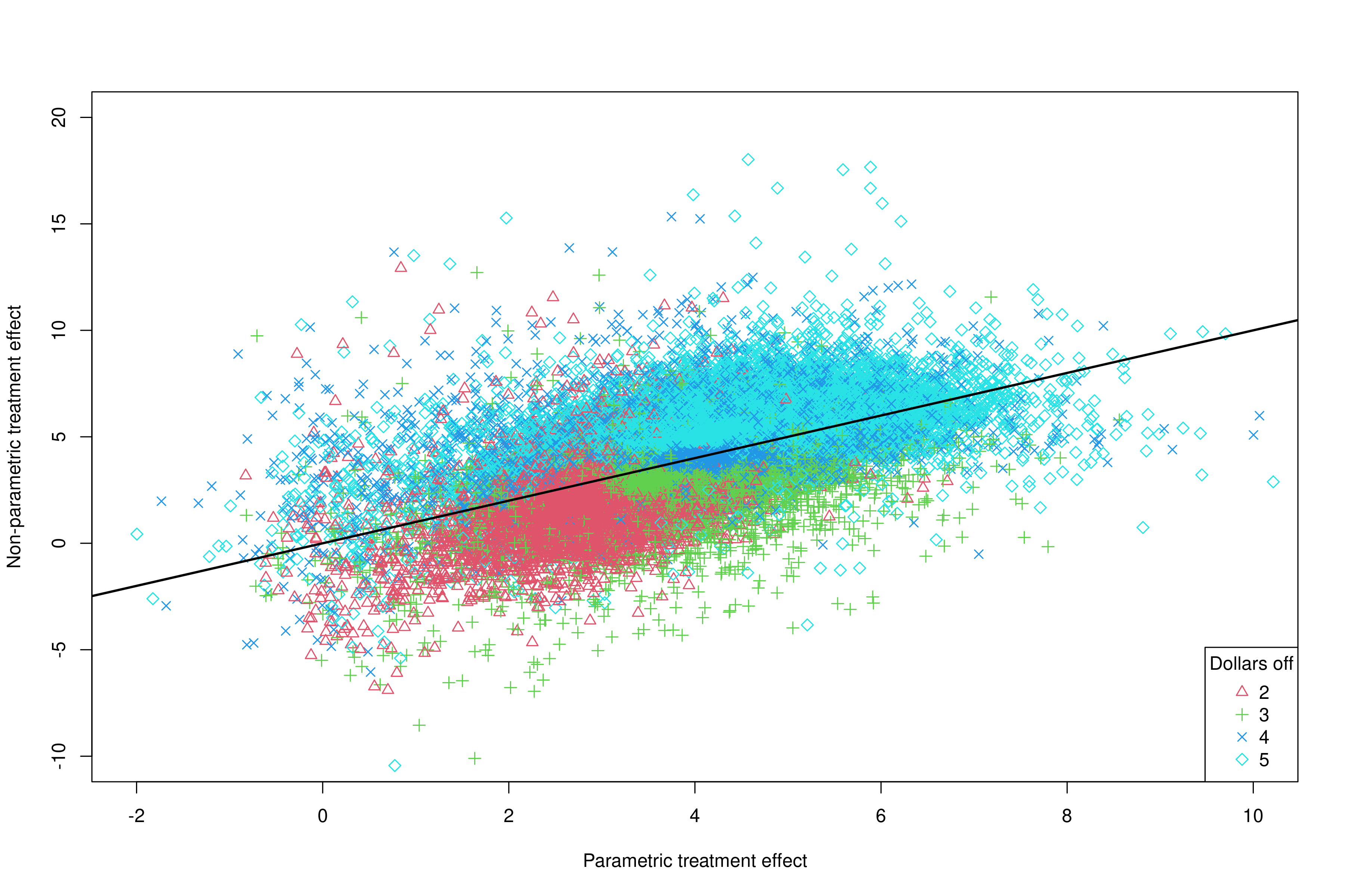
(a) Dollar off promotion

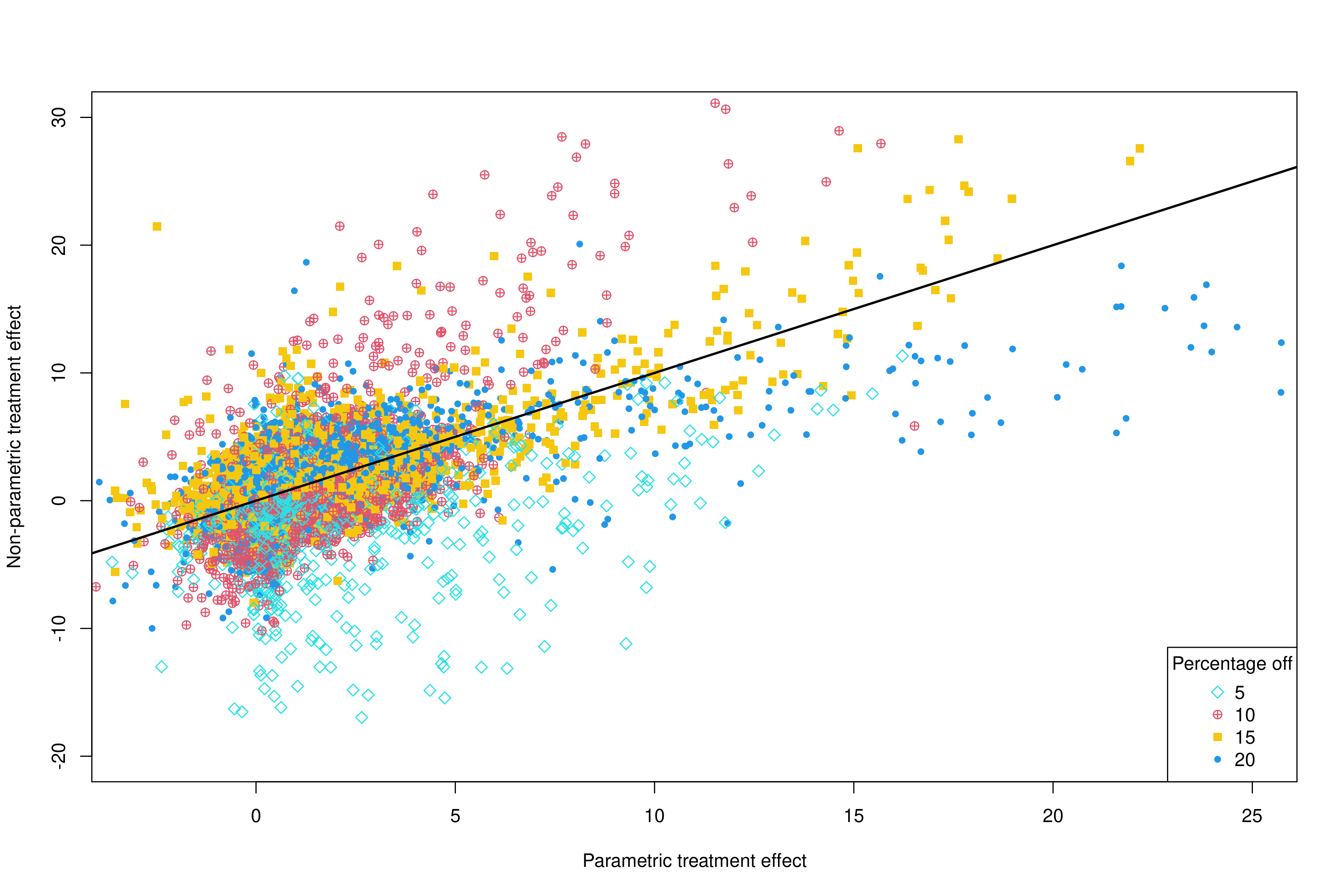
(b) Percentage off promotion

Note: Comparison of the predicted treatment effect from the CATE parameterization (Equation 23) in the holdout treatment to its non-parameteric estimate. The dollar off and percentage off promotions are plotted separately. Each point represents an individual assigned a dollar off or percentage off promotion in the field experiment. The shape and color of the points represents which treatment arm was assigned to the individual. A $45$ degree line is provided as a visual reference.

References

- Ansari and Mela (2003) Ansari, A. and C. F. Mela (2003): “E-Customization,” Journal of Marketing Research, 40, 131–145.
- Arora et al. (2008) Arora, N., X. Dreze, A. Ghose, J. D. Hess, R. Iyengar, B. Jing, Y. Joshi, V. Kumar, N. Lurie, S. Neslin, S. Sajeesh, M. Su, N. Syam, J. Thomas, and Z. J. Zhang (2008): “Putting one-to-one marketing to work: Personalization, customization, and choice,” Marketing Letters, 19, 305–321.
- Ascarza (2018) Ascarza, E. (2018): “Retention Futility: Targeting High-Risk Customers Might be Ineffective,” Journal of Marketing Research, 55, 80–98.
- Athey and Imbens (2016) Athey, S. and G. Imbens (2016): “Recursive partitioning for heterogeneous causal effects,” Proceedings of the National Academy of Sciences of the United States of America, 113, 7353–7360.
- Athey et al. (2019) Athey, S., J. Tibshirani, and S. Wager (2019): “Generalized random forests,” Annals of Statistics, 47, 1179–1203.
- Athey and Wager (2021) Athey, S. and S. Wager (2021): “Policy Learning With Observational Data,” Econometrica, 89, 133–161.