The structure of cluster merger shocks: turbulent width and the electron heating timescale

Abstract

We present a new $2\rm\;Ms$ Chandra observation of the cluster merger Abell 2146, which hosts two huge $M{\sim}2$ shock fronts each ${\sim}500\rm\;kpc$ across. For the first time, we resolve and measure the width of cluster merger shocks. The best-fit width for the bow shock is $17\pm 1\rm\;kpc$ and for the upstream shock is $10.7\pm 0.3\rm\;kpc$. A narrow collisionless shock will appear broader in projection if its smooth shape is warped by local gas motions. We show that both shock widths are consistent with collisionless shocks blurred by local gas motions of $290\pm 30\hbox{$\rm\;km\rm\;s^{-1}\,$}$. The upstream shock forms later on in the merger than the bow shock and is therefore expected to be significantly narrower. From the electron temperature profile behind the bow shock, we measure the timescale for the electrons and ions to come back into thermal equilibrium. We rule out rapid thermal equilibration of the electrons with the shock-heated ions at the $6\sigma$ level. The observed temperature profile instead favours collisional equilibration. For these cluster merger shocks, which have low sonic Mach numbers and propagate through a high $\beta$ plasma, we find no evidence for electron heating over that produced by adiabatic compression. Our findings are expected to be valid for collisionless shocks with similar parameters in other environments and support the existing picture from the solar wind and supernova remnants. The upstream shock is consistent with this result but has a more complex structure, including a $\sim 2\rm\;keV$ increase in temperature ${\sim}50\rm\;kpc$ ahead of the shock.

1 Introduction

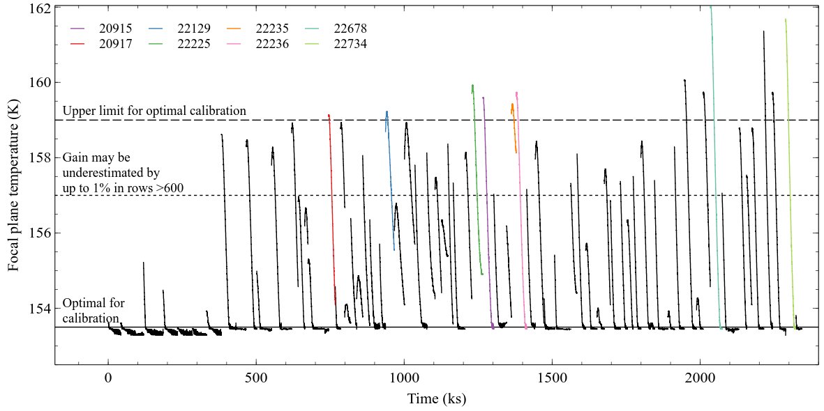
Figure 1: Focal-plane temperature over time for each observation, where the observation start times have been modified to continue from the end of the previous observation. The first 8 observations were taken from August to October 2010 when Chandra’s thermal performance was more stable. Observations which were noted in validation and verification to have periods of higher than optimal focal-plane temperature are shown by the coloured lines.

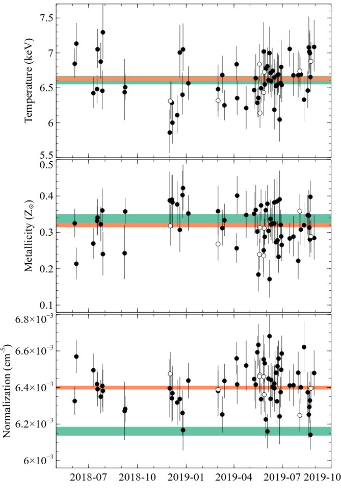
Figure 2: Comparison of the best-fit temperature, metallicity and normalization for a spectrum extracted from a 1.5 arcmin radius region covering most of the cluster emission in each dataset. The green and orange coloured regions show the 1$\sigma$ uncertainties for each parameter from fitting only the 2010 or the new observations, respectively. The white points show the results for the observations that were flagged as having periods of higher than optimum focal-plane temperature.

Major mergers of massive galaxy clusters are the primary hierarchical growth mechanism for clusters (for a review see Markevitch & Vikhlinin 2007). During a merger, the galaxies and dark matter in the clusters behave as nearly collisionless particles (e.g. Clowe et al. 2006) and move unimpeded ahead of the spectacular clash between the hot intracluster atmospheres. X-ray observations of the atmospheric plasma reveal shock fronts, sharp edges associated with cold fronts, large-scale turbulent eddies and tails of gas stripped by ram pressure (e.g. Markevitch 2006). Shocks and turbulence generated by the merger accelerate particles to relativistic speeds. The resulting synchrotron emission produces large-scale radio halos and relics (for a review see van Weeren et al. 2019).

The shocks, with typical Mach numbers $M\sim 1-3$, dissipate most of the merger’s $\sim 10^{64}\rm\;erg$ of kinetic energy (e.g. Sarazin 2002). At low atmospheric densities, shock fronts are believed to be collisionless. The kinetic energy of the inflowing gas is dissipated via plasma-wave interactions between the particles and the magnetic field (e.g. Treumann 2009). Spacecraft travelling through the collisionless solar-wind shock have revealed ions are heated in a narrow shock layer whose width is of order their Larmor radius (e.g. Schwartz et al. 1988). Electrons may remain significantly cooler, equilibrating with the ions via collisions, unless there is an additional electron heating process (for a review see Ghavamian et al. 2013). Chandra observations of merger shocks can map the postshock electron temperature (for a review see e.g. Böhringer & Werner 2010), determine the Mach number and shock speed and thereby measure the electron heating timescale in a single observation (e.g. Markevitch 2006).

Detecting a shock front with a sharp density edge and an unambiguous jump in temperature is rare. Only a handful are known (e.g. Markevitch & Vikhlinin 2007). This is primarily due to an observational shortcoming against detecting well-defined shock fronts. Shock fronts are easiest to detect shortly after the first pericentre passage and if the merger axis is oriented close to the plane of the sky. Only three clusters host shock fronts bright enough for detailed study: the Bullet cluster (Markevitch 2006), Abell 520 (Markevitch et al. 2005; Wang et al. 2018) and Abell 2146. Abell 2146 hosts two $M{\sim}2$ merger shock fronts propagating in opposite directions (Russell et al. 2010, 2012). Although the Bullet cluster shock front has the highest Mach number, the gas temperature (${>}30\rm\;keV$) is difficult to constrain with Chandra’s lower energy range. Abell 520 hosts a weaker shock front. Its postshock gas is permeated with substructure related to the disintegrating subcluster cool core, which must be carefully masked out (Wang et al. 2018). Abell 2146 hosts the two brightest and cleanest shock fronts at measurable temperatures and was therefore the recent target of a Chandra legacy-class observation of a cluster merger.

Here we present the new $2\rm\;Ms$ Chandra observation of Abell 2146. We discuss new structures revealed in this deep dataset and focus on the detailed structure of the shock fronts and on measuring the electron-ion thermal equilibration timescale. Detailed analyses of the break up of the cool cores, constraints on the rate of conduction and level of turbulence will be covered in separate papers. We assume $H_{0}=70\hbox{$\hbox{$\rm\;km\rm\;s^{-1}\,$}\rm\;Mpc^{-1}\,$}$, $\Omega_{\mathrm{m}}=0.3$ and $\Omega_{\Lambda}=0.7$, translating to a scale of $3.7\rm\;kpc$ per arcsec at the redshift $z=0.234$ of Abell 2146 (Struble & Rood 1999; Böhringer et al. 2000). All errors are $1\sigma$ unless otherwise noted.

2 Data reduction

The new Chandra observation of the cluster merger Abell 2146 has an exposure time of $1.93\rm\;Ms$ split over 67 separate observations on the ACIS-I detector between June 2018 and August 2019. When combined with the earlier ACIS-I observations taken in 2010 (Russell et al. 2012), the total exposure is $2.31\rm\;Ms$ (Table 1). All 75 data sets were reprocessed following standard reduction procedures using ciao v4.13 and caldb v4.9.4 provided by the Chandra X-ray Center. These include the latest calibration measurements and crucial updates to the ACIS contaminant model. Improved background screening provided by VFAINT mode was applied to all observations. Background light curves were extracted from neighbouring CCDs and filtered using the lc_clean script to remove periods affected by flares. The net exposure times are given in Table 1. Only obs. ids 20921 and 21674 were affected significantly by flares.

Abell 2146 is located at high ecliptic latitude (declination $+66\deg$) and is therefore at a thermally unfavourable pitch angle for Chandra, which has an ageing exterior thermal finish. This deep image was divided into short observations over a long time period. Several datasets were taken when the focal-plane temperature exceeded the upper limit for optimum calibration of the ACIS gain and spectral resolution. Fig. 1 shows the focal-plane temperature over time. The contrast between the observations taken in 2010, when Chandra’s thermal performance was more stable, and the new observations is clear.

Whilst the majority of the observing time was conducted with the optimal focal-plane temperature, we compared the spectral results from different datasets to search for any systematic effect. Fig. 2 shows the best-fit temperature, metallicity and normalization for the new observations (for an absorbed apec model, see section 4). All are consistent, given the uncertainties, with the equivalent results from the 2010 observations. No systematic differences are found for the observations with higher than optimum focal-plane temperature. We compared the best-fit parameters for the new and old observations from 2010 for key regions, such as the profiles across the shock fronts. The temperature and metallicity values were consistent within the uncertainties (Fig. 2). Normalizations appear on average a few per cent higher for the new datasets. Electron densities derived from these will be ${\sim}2\%$ higher. This small systematic uncertainty is likely due to the escalating contaminant correction but has minimal impact on our results. The new datasets are also likely to be affected by small gain changes (see e.g. Sanders et al. 2014). We conclude that the calibration is sufficient for our analysis.

The absolute astrometry of each dataset was corrected by cross-matching point sources across the separate observations. The final event files were reprojected to match the position of obs. ID 21733. Exposure maps were generated for each observation using energy weights determined from an absorbed apec model at the global cluster temperature of $6.67\pm 0.03\rm\;keV$, metallicity $0.319\pm 0.006\hbox{$\thinspace\mathrm{Z}_{\odot}$}$ (relative to solar abundances defined by Anders & Grevesse 1989 for comparison with previous results) and redshift 0.234. The absorption was fixed to the Galactic value $n_{\mathrm{H}}=3.0\times 10^{20}\hbox{$\rm\;cm^{-2}\,$}$ (Kalberla et al. 2005).

Blank sky backgrounds were generated for each observation. Each processed identically, reprojected to the corresponding sky position, and normalized to match the count rate in the $9.5$–$12\rm\;keV$ energy band. Following Vikhlinin et al. (2005), we tested additional emission models to account for residual background emission after the blank sky backgrounds were subtracted. Soft X-ray background residuals due to Galactic foreground were modelled by a $0.18\rm\;keV$ apec component with solar metallicity. Residual unresolved cosmic X-ray background (CXB) was modelled with an absorbed powerlaw with $\Gamma=1.5$. The best-fit background model parameters were determined for each observation using a spectrum extracted from a large source-free region of the chip. The normalizations of the soft and unresolved CXB components were consistent with zero within the uncertainties for all observations. We therefore proceeded with the blank sky background spectra without using additional spectral models.

3 Image analysis

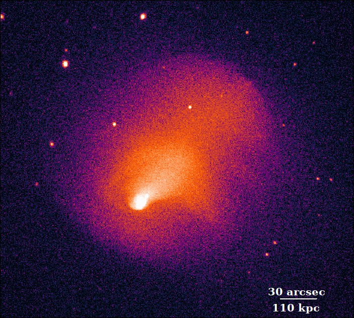
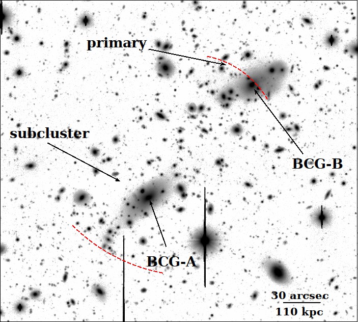
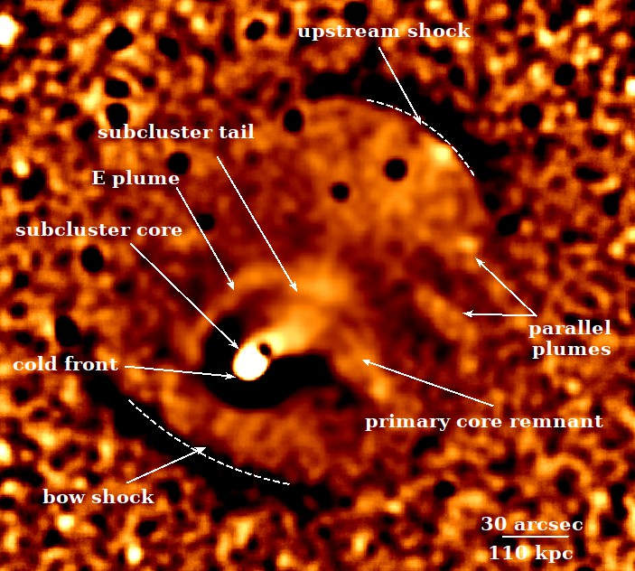
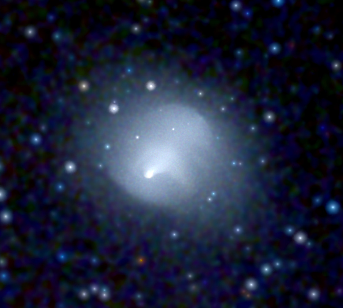
Figure 3: Upper left: Exposure-corrected X-ray image of Abell 2146 in the $0.5$–$4\rm\;keV$ energy band ($\rm\thinspace counts\hbox{$\rm\;cm^{-2}\,$}\hbox{$\rm\;s^{-1}\,$}\hbox{$\rm\;pixel^{-1}\,$}$). Upper right: Subaru R-band optical image showing the primary and subcluster galaxies (King et al. 2016). Lower left: Unsharp-masked image highlighting structure. The shock front locations determined from surface brightness profile fitting are shown by the arcs. The exposure-corrected image, optical image and unsharp-masked image cover the same field of view. Lower right: An RGB image covering a larger field of view with red for $0.5$–$1.5\rm\;keV$, green for $1.5$–$2.5\rm\;keV$ and blue for $2.5$–$6\rm\;keV$. An adaptive smoothing method has been applied to this image (Sanders et al. 2021).

Fig. 3 (upper left) shows an exposure-corrected image of Abell 2146 for the energy range $0.5$–$4\rm\;keV$. The subcluster’s cool core is the brightest and densest region in the cluster and is trailed by a long tail of ram pressure stripped gas that extends over $200\rm\;kpc$. Based on this extended tail and the bow shock location to the SE, the subcluster is currently travelling SE. The primary cluster lies primarily to the NW of the subcluster’s tail with a second shock to the far NW. A comparison of the X-ray and optical images in Fig. 3 (upper left and right) reveals the separation of the subcluster (SE) and primary cluster galaxies (NW) with the bulk of the X-ray emission located between them. Based on the X-ray structure, galaxy distribution and hydrodynamical simulations, Abell 2146 is a collision between two clusters observed ${\sim}0.1\rm\;Gyr$ after the subcluster passed through the primary cluster’s centre.

The merger axis likely runs approximately NW to SE through the centre of the two galaxy distributions. The primary cluster’s cool core has been destroyed in the collision and the remains have spread perpendicular to the merger axis to the SW (referred to in Russell et al. (2012) as the SW plume). Additional plumes are revealed in the new observations to the E of the subcluster’s core (E plume) and NW of the primary cluster’s main remnant (parallel plumes). These structures are clearly seen in the RGB image, which covers a larger field of view and reveals the more extended cluster atmosphere including the preshock gas beyond each shock front (Fig. 3).

Hydrodynamical simulations show that this was likely an off-axis merger with the two cluster cores passing ${\sim}100\rm\;kpc$ from each other at closest approach. This scenario is consistent with the asymmetry in the primary core remnant about the merger axis (Chadayammuri et al. 2022). Dynamical analyses using galaxy line of sight velocities indicate that the merger axis is inclined at only $13$–$19\deg$ to the plane of the sky. This orientation is consistent with the clear shock front detections in the X-ray observations (Canning et al. 2012; White et al. 2015).

The subcluster’s dense core drives a broad bowshock, ${\sim}500\rm\;kpc$ across, seen as a sharp edge in the X-ray surface brightness ${\sim}150\rm\;kpc$ ahead (SE) of the leading edge of the core. The second shock front, the upstream shock, is located at the far NW edge of the primary cluster and is propagating in the opposite direction. The upstream shock forms when material stripped from the subcluster’s core is swept upstream and collides with remaining infalling material. Hydrodynamical simulations indicate that the structure in this region is complex and sensitive to the merger parameters. The upstream shock evolves rapidly. Its curvature is variable as it propagates through a clumpy medium falling in behind the subcluster. In addition, simulations show additional shocks and shock-heated structures in this region (e.g. Chadayammuri et al. 2022).

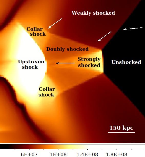
Figure 4: Temperature slice from the hydrodynamical simulations by Chadayammuri et al. (2022) showing the upstream shock structure in detail. The merger axis is oriented left to right and the upstream shock propagates from left to right. The arrows show the approximate flow direction at various positions. The colour bar shows the temperature in K.

Fig. 4 shows the main features of the complex flow that feeds the upstream shock in a temperature slice from the hydrodynamic models of Chadayammuri et al. (2022). While the slice is taken from their best matching model, these features are robust to parameter changes, as can be seen in Fig. 9 of that paper. The coolest material at the right hand edge is unshocked gas from the subcluster, which falls supersonically towards the primary cluster. This material flows leftward and converges toward the merger axis under the primary cluster’s gravitational potential. This results in a series of strong, normal and weaker, inclined shock fronts. The upstream shock structure is expected to be particularly complex. In addition, it is projected onto the break up of the primary cluster’s core.

Structure in the X-ray surface brightness edges can be highlighted by subtracting smoothed images. Fig. 3 (lower left) shows an unsharp-masked image, where an exposure-corrected image smoothed with a 2D Gaussian of $\sigma=10\rm\;arcsec$ has been subtracted from a similarly smoothed image where $\sigma=2.5\rm\;arcsec$. The order of magnitude drop in surface brightness across the contact discontinuity or cold front on the leading edge of the subcluster core appears particularly prominent. The primary core remnant is fully revealed and extends ${\sim}250\rm\;kpc$ from the merger axis. On the opposite side of the merger axis, the deeper observation reveals an E plume that curves from the end of the subcluster’s tail almost to the E edge of the subcluster’s core. Hydrodynamical simulations suggest that this structure is unrelated to the break up of the primary cluster’s core (Chadayammuri et al. 2022) but instead may be a large turbulent eddy.

The deeper observation also shows new structure through the primary cluster. The bright nib on the leading edge of the upstream shock is coincident with the primary cluster’s brightest cluster galaxy (BCG-B). Gas clumps attached to and stripped from the massive galaxies in the primary cluster lie between the upstream shock and the end of the subcluster’s tail. To the SW of the collision site, two further plumes extend perpendicular to the merger axis and parallel to the primary core remnant. These plumes are also visible in the raw image.

4 Spatially resolved spectroscopy

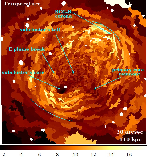
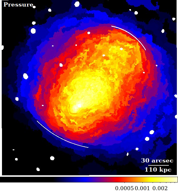
Figure 5: Left: Projected temperature map (keV). Right: Projected pseudo-pressure map ($\rm\;keV\rm\;cm^{-5/2}\hbox{$\rm\;arcsec^{-2}\,$}\,$). The excluded point sources are visible as small white circles. The shock front locations determined from surface brightness profile fitting are shown by the arcs.

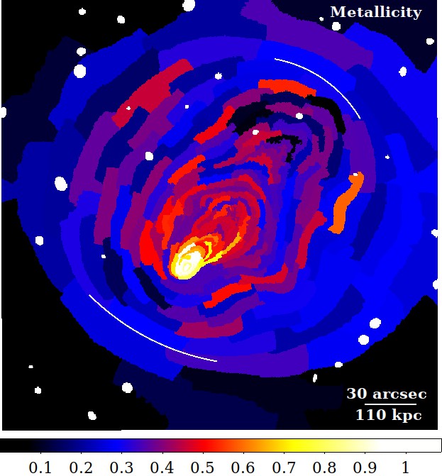
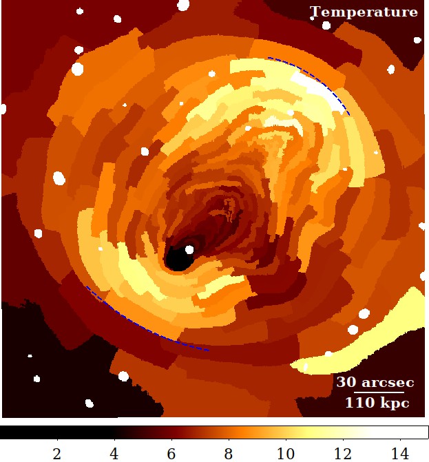
Figure 6: Left: Metallicity map (Z_⊙). Right: Projected temperature map (keV) for matching spatial binning. The excluded point sources are visible as small white circles.

Detailed maps of the gas temperature, metallicity, normalization and pressure were produced with a contour binning algorithm (Sanders 2006). Contour binning generates spatial regions by grouping together neighbouring pixels with similar surface brightness. Pixels are added to each region until a specified signal-to-noise ratio is reached. The dimensions of the regions were restricted so that their length was at most two and a half times their width.

For each observation, spectra were extracted from each contour binning region and appropriate responses were generated. To ensure sufficient counts, a single blank sky background for each dataset was extracted from an on-axis region with radius $1.5\arcmin$. The spectra were grouped to ensure a minimum of 1 count per spectral channel. For each region, spectra from all observations were fit simultaneously over the energy range $0.5$–$7\rm\;keV$ in xspec v.12.11.1 (Arnaud 1996) with an absorbed thermal plasma emission model (phabs(apec); Smith et al. 2001).

X-ray spectral modelling of cluster plasma is particularly straightforward (for a review see e.g. Böhringer & Werner 2010). All radiative processes depend on the collision of an electron and an ion. Due to the low density, all excited ions radiatively de-excite before another collision occurs. The low density ensures all photons escape the cluster. Radiative transfer calculations are not required.

Thermal plasma emission models, such as apec, are generated by summing over all electron ion collision rates. The collision rates are dependent on the temperature, electron density and ion density. The normalization of the spectrum is proportional to the electron and ion densities. The shape of the spectrum is determined by the electron temperature and heavy element abundances, typically measured from line emission. At temperatures above a few keV, the electron temperature is predominantly constrained by the exponential dropoff in the bremsstrahlung continuum shape at high energies. In contrast, the emission in a low energy band, such as $0.5$–$4\rm\;keV$, is largely independent of temperature. We note that for gas temperatures below ${\sim}3\rm\;keV$, the prominence of Fe L emission at ${\sim}1\rm\;keV$ provides a sensitive temperature diagnostic. The apec model therefore has three free parameters: temperature, metallicity and normalization. Additional parameters for the redshift and absorption were fixed to 0.234 and the Galactic value of column density $n_{\mathrm{H}}=3.0\times 10^{20}\hbox{$\rm\;cm^{-2}\,$}$ (Kalberla et al. 2005), respectively.

This model assumes that the electrons are in thermal Maxwellian equilibrium and the ions are in thermal ionization equilibrium. While it is true that on microphysical scales kinetic effects and temperature anisotropies are important (as attested by lab experiments and heliospheric observations), on astronomical scales the fluid description is well-motivated. Kinetic simulations of shocks (e.g. Caprioli & Spitkovsky 2014a; Park et al. 2015) show that distributions are indeed Maxwellian when integrated on scales of hundreds of ion gyroradii (${>}10^{12}\rm\;cm$ for the ICM). For Chandra’s CCD spectral resolution (${\sim}100\rm\;eV$), differences in the electron and ion temperatures will not significantly affect the measured parameters. In future, X-ray microcalorimeters (onboard e.g. Athena, Nandra et al. 2013) with spectral resolution of a few eV will detect thermal line broadening and thereby separately constrain the ion temperature (Hitomi Collaboration et al. 2016). Similarly, detailed measurements of the intensity ratios of Fe K$\alpha$ lines with X-ray microcalorimeters will be able to detect a non-equilibrium ionization state (e.g. Akahori & Yoshikawa 2010, 2012; Wong et al. 2011).

We therefore proceed with the absorbed thermal plasma emission model as described and determine the best-fit spectral model by minimizing the C-statistic (Cash 1979). The best-fit spectral parameters were painted onto the contour bin regions to make maps in temperature and metallicity. Pseudo-pressure was generated by multiplying the temperature and square root of the normalization.

For maps with S/N$=32$ (Fig. 5), the uncertainties are typically ${\sim}15\%$ in temperature, ${\sim}8\%$ in normalization and ${\sim}18\%$ in pressure. Regions at lower temperatures, such as the subcluster’s core and tail, have smaller uncertainties in temperature at $5\%$ and $10\%$, respectively. This improvement is due to the temperature sensitivity of the Fe L line emission, which is prominent at low X-ray temperatures. The uncertainties in temperature increase to ${\sim}20\%$ in the postshock gas at $8$–$10\rm\;keV$. These higher temperatures are difficult to constrain because the exponential cut off in the bremsstrahlung continuum emission lies beyond Chandra’s energy range.

Fig. 5 shows the resulting maps of gas temperature and pressure. The pressure peaks in the subcluster’s cool core and is elongated along the merger axis toward the upstream shock. The temperature map reveals the ${\sim}2\rm\;keV$ gas along the leading edge of the subcluster’s cool core and the steady increase to ${\sim}8\rm\;keV$ through the ram pressure stripped tail. The gas behind each shock front has been heated to ${\sim}10\rm\;keV$. The primary cluster’s core is visible as a relatively cool plume at ${\sim}6\rm\;keV$, which is ${\sim}2\rm\;keV$ cooler than the surrounding gas. Similarly, the E plume is cooler ($6$–$7\rm\;keV$) than the surrounding medium at $8\rm\;keV$. The temperature map indicates a break in the E plume in a hot region at $9.5\rm\;keV$ covering roughly $6\arcsec\times 10\arcsec$. This region is coincident with a drop in the X-ray surface brightness. The parallel plumes also appear cooler than the ambient by ${\sim}0.5\rm\;keV$. The bright nib on the leading edge of the upstream shock, associated with BCG-B, appears cooler than the surrounding shock-heated gas by at least $5\rm\;keV$. This is likely to be the remains of the massive galaxy’s hot atmosphere, or corona, that has survived ram pressure stripping. The break up and detailed structure of the cool cores will be discussed further in separate papers.

         

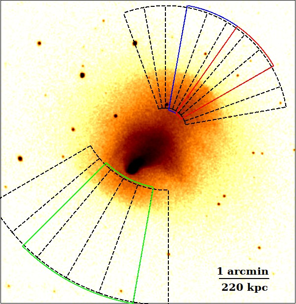
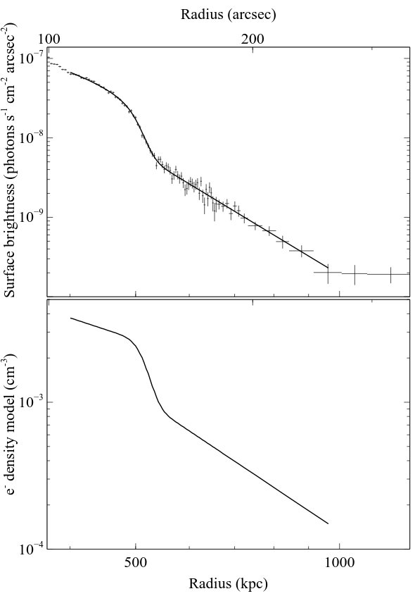
Figure 7: Left: Image with $10^{\circ}$-wide sectors overlaid for the bow shock (SE, $210$–$270^{\circ}$) and the upstream shock (NW, $10$–$110^{\circ}$), where angles are measured anti-clockwise from W. Note that the overlapping sectors, $+5^{\circ}$ on those shown, are not included for clarity. Broad sectors for the bow shock (SE, $225$–$260^{\circ}$, green) and the upstream shock (NW, $30$–$55^{\circ}$, red, and $55$–$80^{\circ}$, blue) are also shown with small position offsets for clarity. Upper right: Surface brightness profile and best-fit model for a sector from $225$–$260^{\circ}$ at the bow shock. Lower right: Corresponding deprojected electron density model.

For the lower spatial resolution maps with S/N$=72$ (Fig. 6), the uncertainties are typically $5\%$ in temperature and $15$–$20\%$ in metallicity. Similarly to the S/N$=32$ maps, the uncertainties are lower in the cool core where the Fe L line emission provides tighter constraints on temperature and metallicity. The uncertainties are also higher in the postshock regions where the gas is almost fully ionized and there is little line emission. This effect can be clearly seen in Fig. 6 in the shock-heated region behind the upstream shock where there are several regions with very low, essentially unconstrained, metallicity.

Fig. 6 shows a clear peak at roughly solar metallicity in the subcluster’s cool core. Metallicity is enhanced at levels of $0.4$–$0.6\hbox{$\thinspace\mathrm{Z}_{\odot}$}$ through the ram-pressure stripped tail and the E plume. The metallicity is ${\sim}0.25\hbox{$\thinspace\mathrm{Z}_{\odot}$}$ beyond this for the bulk of the cluster atmosphere. The subcluster’s cool core has likely been enriched by stellar winds and supernovae in BCG-A. This material is then stripped from the cool core and mixes with the lower metallicity ambient medium to produce a steady decline in measured metallicity through the tail. The primary cluster’s cool core does not have such a clear metallicity peak. The metallicity structure of the cool cores will be examined in more detail in a separate paper.

5 Shock structure

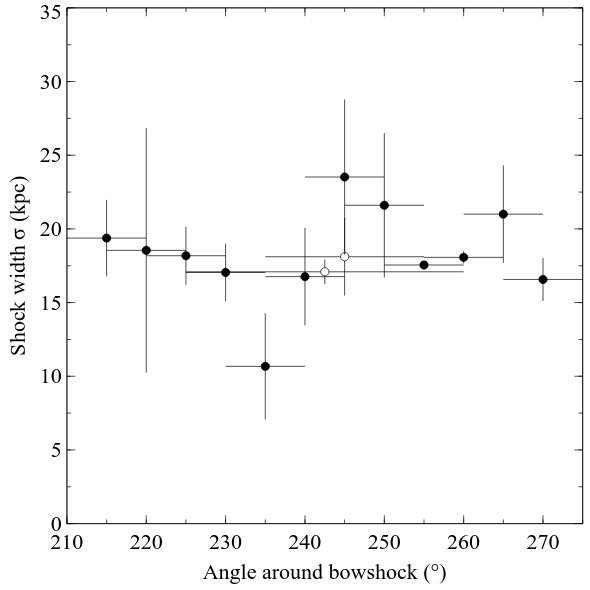
Figure 8: The best-fit Mach number, shock position and shock width parameters determined from fitting the projected density jump model to surface brightness profiles extracted in $10^{\circ}$ sectors around the bow shock front (solid points). The expected $\mathrm{cos}\theta$ dependence of the Mach number (see text) is shown by the dashed line. The best-fit parameters do not vary significantly for a $225$–$260^{\circ}$ sector or a narrower $235$–$255^{\circ}$ sector (open points), which was selected for subsequent analysis of the temperature and density structure of the shock.

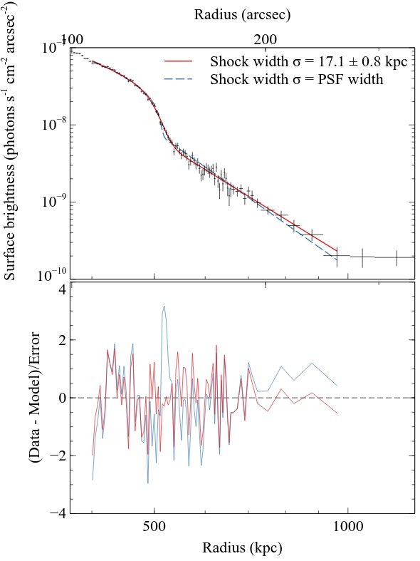
Figure 9: Upper: Surface brightness profile across the bow shock front with the best-fit model for a projected density jump of width $\sigma$ (solid red line). The best-fit model for a projected jump with zero width convolved with a Gaussian with $\sigma=1\rm\;arcsec$ to approximate the Chandra PSF is shown for comparison. Lower: Residuals calculated by subtracting each best-fit model from the observed surface brightness profile and dividing the result by the uncertainties.

Fig. 7 shows $10^{\circ}$-wide sectors used to extract surface brightness profiles across the bow and upstream shock fronts. Overlapping $10^{\circ}$-wide sectors, offset in angle by $5^{\circ}$ from those shown, were also used. The regions were positioned to align with the centre and curvature of each respective surface brightness edge. The analysis was repeated with modest offsets in the region position and the surface brightness profile modelling results were found to be robust. Each sector was divided into radial bins of $1\rm\;arcsec$ width, increasing to $2.5\rm\;arcsec$ and larger for radii greater than $100\rm\;kpc$ beyond the surface brightness edge where the background dominates. This procedure ensured at least 30 source counts are contained in each radial bin for the resulting surface brightness profiles. Point sources were excluded. The background was subtracted using the surface brightness measured in source-free regions beyond each sector. The energy range was restricted to $0.5$–$4\rm\;keV$ to minimise the temperature dependence of the profile (section 4; see e.g. Churazov et al. 2016) and maximise S/N at the shock fronts. The density jump across each shock front is therefore determined essentially independent of the temperature change (see e.g. Markevitch & Vikhlinin 2007).

Each surface brightness profile was fitted with a model for a projected density jump (Fig. 7). This model consists of a power law for the preshock gas density, a second power law for the postshock gas density and a sharp density jump at the shock edge convolved with a Gaussian function of width $\sigma_{\mathrm{sh}}$. The model has six free parameters: the slopes ($\alpha_{1}$, $\alpha_{2}$) and normalizations ($\rho_{1}$,$\rho_{2}$) of each power law in electron density, the position of the shock, $R_{\mathrm{sh}}$, and the width of the shock, $\sigma_{\mathrm{sh}}$. The subscripts 1 and 2 denote the preshock (upstream) and postshock (downstream) values, respectively. The density model was projected along the line of sight by assuming the same shock curvature along the line of sight as measured in the plane of the sky. This model was then fitted to the observed surface brightness profiles by minimizing $\chi^{2}$.

Fig. 7 shows the density model and the corresponding surface brightness model overlaid on a surface brightness profile extracted across the bow shock for the broad sector from $225$ to $260^{\circ}$. The projected density jump model is an excellent fit in this sector with $\chi^{2}=75$ for 77 degrees of freedom. The uncertainties on each parameter are calculated by evaluating the best-fit model and parameters for 1000 Monte Carlo realizations of the surface brightness profile. Increasing or decreasing the subtracted background level by $1\sigma$ does not significantly alter the measured parameters. From the best-fit density jump, the shock Mach number is then

$$M=\left(\frac{2\left(\rho_{2}/\rho_{1}\right)}{\gamma+1-\left(\rho_{2}/\rho_{1}\right)\left(\gamma-1\right)}\right)^{1/2},$$ (1)

where the adiabatic index $\gamma=5/3$ for a monatomic gas.

The density model assumes a spherical and steady shock front propagating in the plane of the sky and power-law profiles in gas density in the pre- and postshock gas. This model is most applicable close to the shock front. Therefore, we set an inner radial limit of $400\rm\;kpc$ which excludes substructure around the subcluster’s core. Based on galaxy dynamical measurements and hydrodynamical simulations, the merger axis in Abell 2146 is estimated to be only $13$–$19^{\circ}$ from the plane of the sky (Canning et al. 2012; White et al. 2015; Chadayammuri et al. 2022). This angle is entirely consistent with the clear detection of two sharp shock fronts, which would appear smeared in projection at larger inclination angles. Inclination effects are therefore expected to be minimal.

5.1 Bow shock front

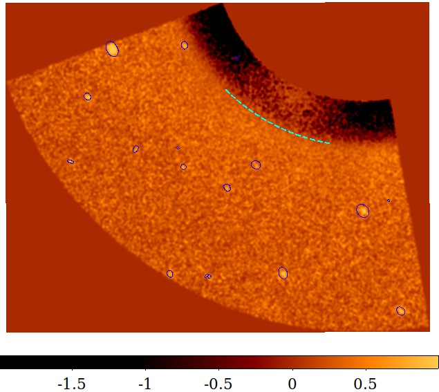
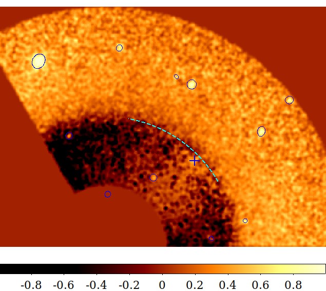
Figure 10: Exposure-corrected images in the $0.5$–$4\rm\;keV$ energy band for the shock sectors with the best-fit projected density jump model subtracted. The residual images were then normalized by the exposure-corrected image. The colour bar values therefore represent the fractional difference (data - model)/data. Left: Bow shock region where the model was determined for the $225$–$260^{\circ}$ sector. Right: Upstream shock region where the model was determined for the $55$–$80^{\circ}$ sector. Point sources are marked by blue circles and the shock locations are marked by cyan dashed lines. The location of BCG-B is shown by the blue cross (Fig. 3).

Fig. 8 shows the best-fit Mach number, shock radius and shock width as a function of angle around the bow shock front. As expected for an archetypal bow shock, the Mach number peaks at the centre or ‘nose’ of the shock front ($235$–$255^{\circ}$) at $2.44\pm 0.17$. The Mach number declines with angle to $M{<}2$, where the shock becomes oblique. The decline in Mach number appears symmetric; values at equal distances from the shock ‘nose’ are consistent within the uncertainties. If the shock is steady, and the velocity of the preshock medium is uniform, the shock Mach number is expected to vary as $\mathrm{cos}\theta$, where $\theta$ is the angle between the velocity of the subcluster’s core and the normal to the shock front (in Fig. 8, $\theta=0$ at approximately $245\deg$). Fig. 8 shows that the angular dependence is much steeper than this expectation. This indicates that the shock velocity is not steady and the preshock medium is not uniform. We note that if the motion of the subcluster’s core was not in the plane of the sky, the angular dependence would be shallower so this does not explain the discrepancy.

In general, the measured shock properties, including the Mach number, do not vary significantly for a broad sector across the centre of the shock front ($225$–$260^{\circ}$, Fig. 7 and 8). This sector is therefore used to evaluate the imaging and spectral parameters across the shock front because it probes the narrow region of the normal shock and captures a sufficient number of photons. We note that an even more conservative sector selection of $235$–$255\deg$ produces consistent results.

For the first time, we resolve and measure the width of a cluster merger shock front. For the $225$–$260^{\circ}$ sector, the width is $17\pm 1\rm\;kpc$ and measurements in all sectors are consistent with this value within the uncertainties. Fig. 9 shows that this width is clearly preferred over an unresolved width with $\chi^{2}=75$ for 77 degrees of freedom compared to $\chi^{2}=100$ for 78 degrees of freedom. Similarly, the position of the shock front is consistent in all sectors, $R_{\mathrm{s}}=516.3\pm 1.3\rm\;kpc$, although the uncertainties increase significantly at large angles where the surface brightness declines. Fig. 9 shows that the Mach number in this large sector $M=2.24\pm 0.09$ from the density jump $r=2.50\pm 0.08$ (Eq. 1). The best-fit shock width of $\sigma_{\mathrm{sh}}=17\pm 1\rm\;kpc$ is significantly preferred over an unresolved width ($\chi^{2}=75$ for 77 degrees of freedom compared to $\chi^{2}=99$ for 78 degrees of freedom). An unresolved shock front is clearly a poor fit around the model’s inflection point with residuals of ${>}3\sigma$ significance at a radius of $520\rm\;kpc$ in the lower panel of Fig. 9.

Fig. 10 shows residual images where the best-fit projected density model for the $225$–$260\deg$ sector has been subtracted from an image covering the shock sector. Whilst this model clearly oversubtracts the postshock emission at large angles where the density jump is smaller, no other significant residuals in pre- or postshock gas are seen. The $225$–$260\deg$ sector appears clear of substructure. We proceeded with this region for the spectral analysis.

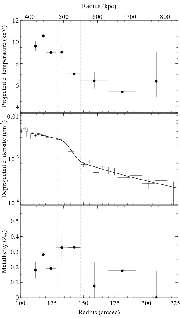
Figure 11: Projected temperature and metallicity profiles extracted in the $225$–$260\deg$ sector across the bow shock front (top and bottom panels). Deprojected electron density profile with the best-fit density jump model (solid black line) overlaid (middle panel). Vertical dashed lines approximate the full width of the density jump and guide the radial binning selected for the temperature profile.

Temperature and metallicity profiles were extracted using the bow shock sector ($225$–$260\deg$; Fig. 7) and wider regions each with ${\sim}3000$ counts spread over 75 datasets. This ensured temperature precision of $10$–$20\%$. As detailed in section 4, spectra and responses were extracted from each region and fitted simultaneously with an absorbed apec model in xspec. Results were consistent when using different radial binning and different subsets of obs. IDs, including comparing the 2010 observations and the new data. Deprojected electron density profiles were produced using the dsdeproj deprojection routine, assuming spherical symmetry to subtract the projected contribution from each successive annulus (Sanders & Fabian 2007; Russell et al. 2008).

Fig. 11 shows the projected temperature, metallicity and deprojected density profiles for the bow shock sector. The shock front is clearly visible as a rapid increase in temperature from ${\sim}6.0\pm 0.6\rm\;keV$ to $9.3\pm 0.2\rm\;keV$. From the density jump and the sound speed in the preshock gas $c_{\mathrm{s}}=1250^{+80}_{-40}\hbox{$\rm\;km\rm\;s^{-1}\,$}$, the shock velocity $v_{\mathrm{sh}}=2800^{+200}_{-100}\hbox{$\rm\;km\rm\;s^{-1}\,$}$. A temperature profile extracted from a sector covering a reduced angular range of $235$–$255\deg$ produced a consistent result within the uncertainties. The deprojected electron density also shows the shock front clearly with a steady increase over ${\sim}40\rm\;kpc$. The increase is consistent with the best-fit width with $\sigma_{\mathrm{sh}}=17\rm\;kpc$. The best-fit metallicity is roughly constant through this sector at $0.24\pm 0.03\hbox{$\thinspace\mathrm{Z}_{\odot}$}$ in the postshock gas and $0.1\pm 0.1\hbox{$\thinspace\mathrm{Z}_{\odot}$}$ in the preshock gas. This difference is not significant given the uncertainty on the preshock metallicity. The temperature profile is analysed in more detail in section 6 where we measure the electron-ion thermal equilibration timescale.

The shock width can be compared with the electron mean free path (Spitzer 1956)

$$\lambda_{\mathrm{e}}{\sim}11\rm\;kpc\left(\frac{T_{\mathrm{e}}}{9\rm\;keV}\right)^{2}\left(\frac{n_{\mathrm{e}}}{2.3\times 10^{-3}\hbox{$\rm\;cm^{-3}\,$}}\right)^{-1},$$ (2)

where $T_{\mathrm{e}}$ is the electron temperature and $n_{\mathrm{e}}$ is the electron density. For the bow shock front, $\lambda_{\mathrm{e}}=11\pm 2\rm\;kpc$ (Fig. 12), which is similar to the shock width. A collisional shock should have a width roughly a few times the mean free path. Any deformation of the shock shape across the large sector analysed would increase the width further. The bow shock therefore appears too narrow for a collisional shock.

Instead, the bow shock is likely a collisionless shock with width of order the ion gyroradius (typically npc). Small scale turbulent eddies in the preshock region will warp the shape of this narrow shock. These local gas motions modulate the shock speed to produce an uneven shock surface, which appears broader when seen in projection.

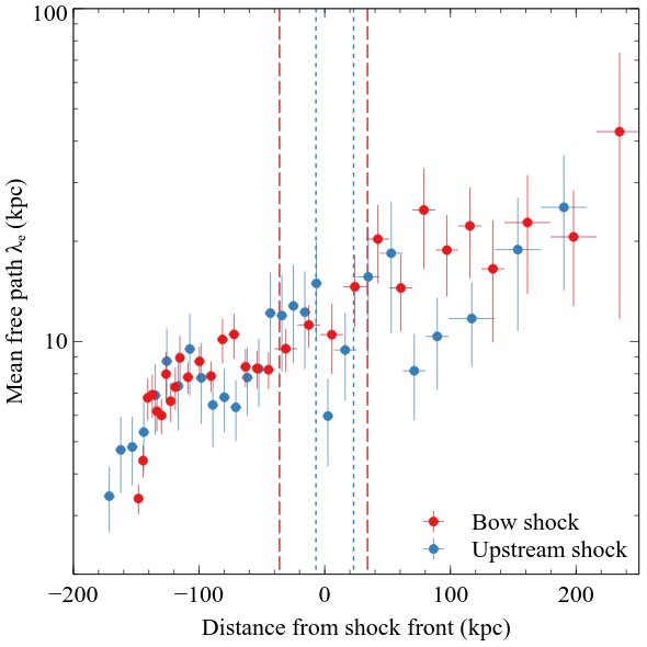
Figure 12: Electron mean free path across the bow and upstream shock fronts.

The width of the shock front will grow due to turbulence if the shock front is not driven by the subcluster’s core and instead propagates freely (Nulsen et al. 2013). During the infalling leg of the merger, the core accelerates and drives the shock front. The standoff distance of the shock agrees with the expectation for a steady shock (Zhang et al. 2019). For a $M{\sim}2$ shock, that distance is ${\sim}0.4$ times the radius of the core. Pressure fluctuations propagate slowly into the high density subcluster’s core compared to the surrounding hot atmosphere. The leading edge of the subcluster’s core is essentially rigid. During infall, velocity perturbations on scales comparable to or greater than the subcluster’s core radius will cause only modest fluctuations in the shock standoff distance. Perturbations on smaller scales can cause local displacements in the shock front but these are limited in magnitude by the pressure gradient behind the shock. Therefore, before core passage, perturbations in the shock’s shape due to turbulence are modest.

After the shock detaches from the leading edge of the subcluster’s core, it is no longer driven by a rigid body and displacements in it can accumulate. The observed standoff distance for the bow shock is several times larger than the radius of the core. The merger is therefore observed after core passage. The shock has detached and propagates almost freely.

The rms radial displacements in the shock front ${\Delta}R=\sqrt{Rl}\left(\sigma_{\mathrm{turb}}/v_{\mathrm{sh}}\right)$, where the turbulence rms speed is $\sigma_{\mathrm{turb}}$, the coherence length $l$ is typically ${\sim}0.1R$ and $v_{\mathrm{sh}}$ is the shock speed (Nulsen et al. 2013). For a shock radius $R{\sim}500\rm\;kpc$, width $\sigma{\sim}20\rm\;kpc$ and shock velocity $v_{\mathrm{sh}}=2800^{+200}_{-100}\hbox{$\rm\;km\rm\;s^{-1}\,$}$, we estimate $\sigma_{\mathrm{turb}}=290\pm 30\hbox{$\rm\;km\rm\;s^{-1}\,$}$. This value measured at a radius of a few hundred kpc is consistent with turbulence measured in cluster cores to radii of a few tens of kpc (e.g. Sanders et al. 2011; Hitomi Collaboration et al. 2016). This implies a slow increase in turbulent velocity with radius.

5.2 Upstream shock front

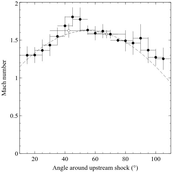
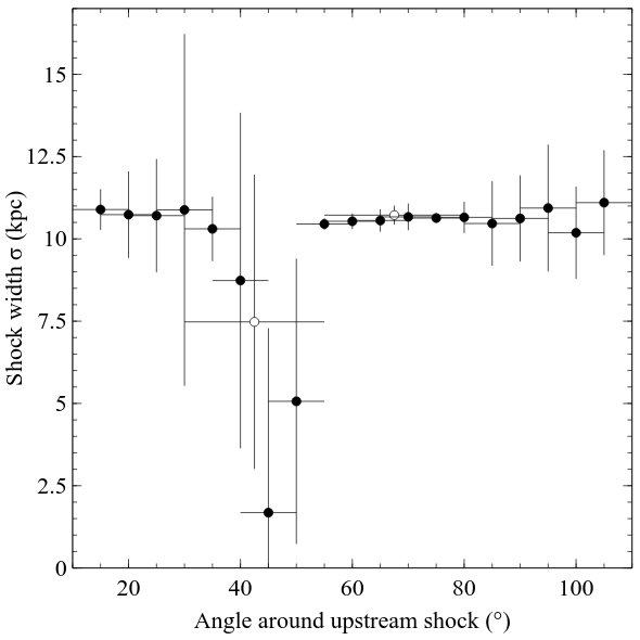
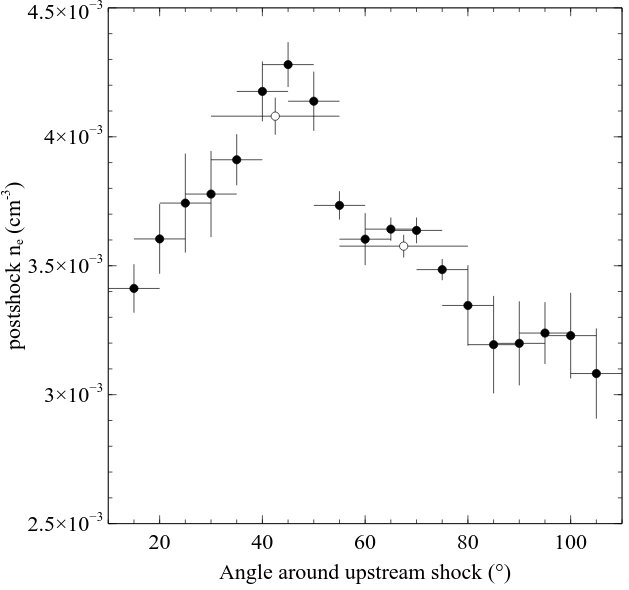
Figure 13: The best-fit Mach number, shock width and postshock electron density parameters determined from fitting the projected density jump model to surface brightness profiles extracted in $10\deg$ sectors around the upstream shock front. The expected $\mathrm{cos}\theta$ dependence of the Mach number (see text) is shown by the dashed line. The $30$–$55\deg$ sector contains trails of ram pressure stripped gas from the massive galaxies in the primary cluster.

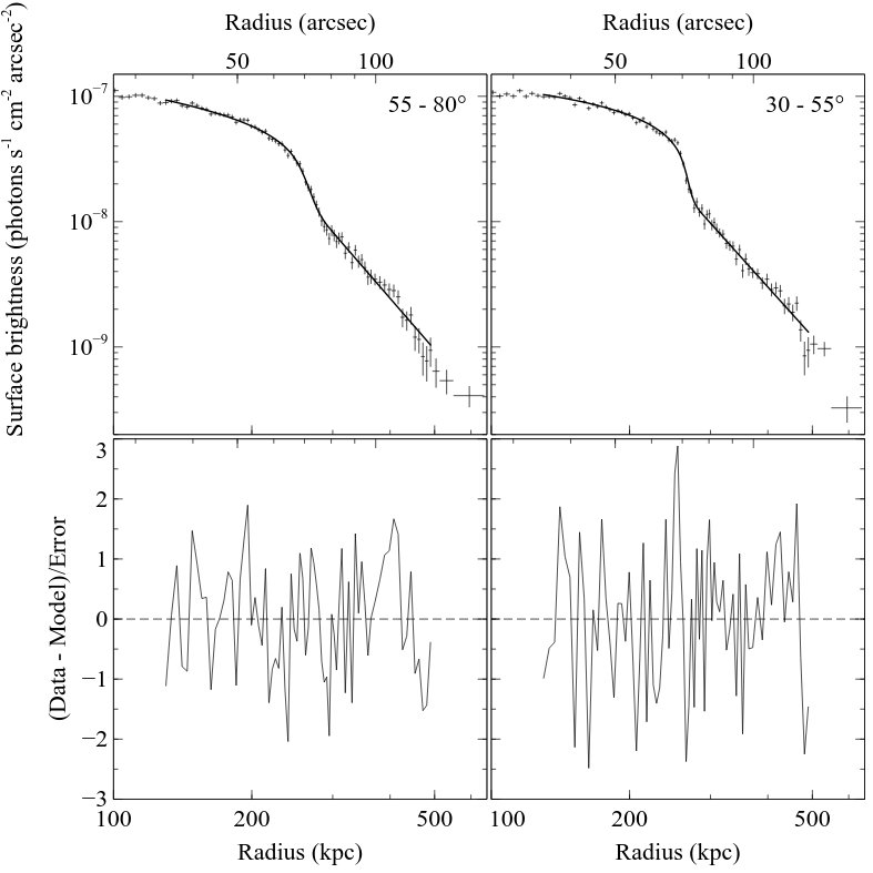
Figure 14: Upper: Surface brightness profiles across the upstream shock front for two sectors ($30$–$55\deg$ and $55$–$80\deg$) with the best-fit model for a projected density jump (solid lines). Lower: Residuals calculated by subtracting the best-fit model from the observed surface brightness profile and dividing the result by the uncertainties.

Using the $10\deg$-wide sectors shown in Fig. 7, we extracted a series of surface brightness profiles across the upstream shock front and fit each with the projected density model described in section 5. Fig. 13 shows the best-fit Mach number, shock width and postshock density as a function of angle around the upstream shock front. Similar to the bow shock front, the Mach number decreases with angle around the shock from a peak at $M=1.58\pm 0.05$. The decline in Mach number with angle is shallower compared to the bow shock and appears to match the expected $\mathrm{cos}\theta$ dependence much more closely (Fig. 13). For the upstream shock, the Mach number drops by $15\%$ over $30^{\circ}$ compared to ${\sim}45\%$ for a similar angular range across the bow shock. Hydrodynamical simulations show the structure of the upstream shock front is complex, rapidly evolving, and sensitive to the merger scenario (Chadayammuri et al. 2022; section 3). Therefore, it seems unlikely that agreement with theoretical expectations is a result of a steady flow and uniform velocity in the preshock medium.

Emission from the galaxy atmospheres, particularly BCG-B, produces a clear artificial spike in the best-fit Mach number and postshock electron density from $30$ to $55\deg$. Comparison of the surface brightness profiles from the $30$–$55\deg$ and $55$–$80\deg$ sectors (Fig. 14), and examination of the residual image (Fig. 10), indicate that ram pressure stripped material from the BCG’s halo is spread over at least $100\rm\;kpc$ throughout this sector. Additional contributions from the halos of other large galaxies in the primary cluster are also likely (Fig. 3). It was therefore not possible to cleanly mask out this emission in the $30$–$55\deg$ sector. The projected density model was a poor fit in this sector, $\chi^{2}=123$ for 73 degrees of freedom compared to $\chi^{2}=68$ for 73 degrees of freedom in the $55$–$80\deg$ sector (Fig. 14). The galaxy halo of BCG-B is also detected as a cool patch in the middle of the upstream shock front in the temperature map (Fig. 5). We therefore proceed by analysing the upstream shock parameters primarily in the $55$–$80\deg$ sector. An analysis of the break up of the cool cores and galaxy halos in the merger will be published separately.

Using the $55$–$80\deg$ sector (Fig. 7), we resolve the width of the upstream shock front. With best-fit width $\sigma_{\mathrm{sh}}=10.7\pm 0.3\rm\;kpc$, the upstream shock is significantly narrower than the bow shock. The upstream shock is sharper than the bow shock even in the raw images (Fig. 3), which is consistent with this result. The measured shock width is consistent in all $10^{\circ}$ sectors, although the uncertainty is particularly large from $30$–$55^{\circ}$ as expected given the substructure (Fig. 13). The Mach number in this large sector $M=1.58\pm 0.05$ from the best-fit density jump $r=1.82\pm 0.07$ (Eq. 1).

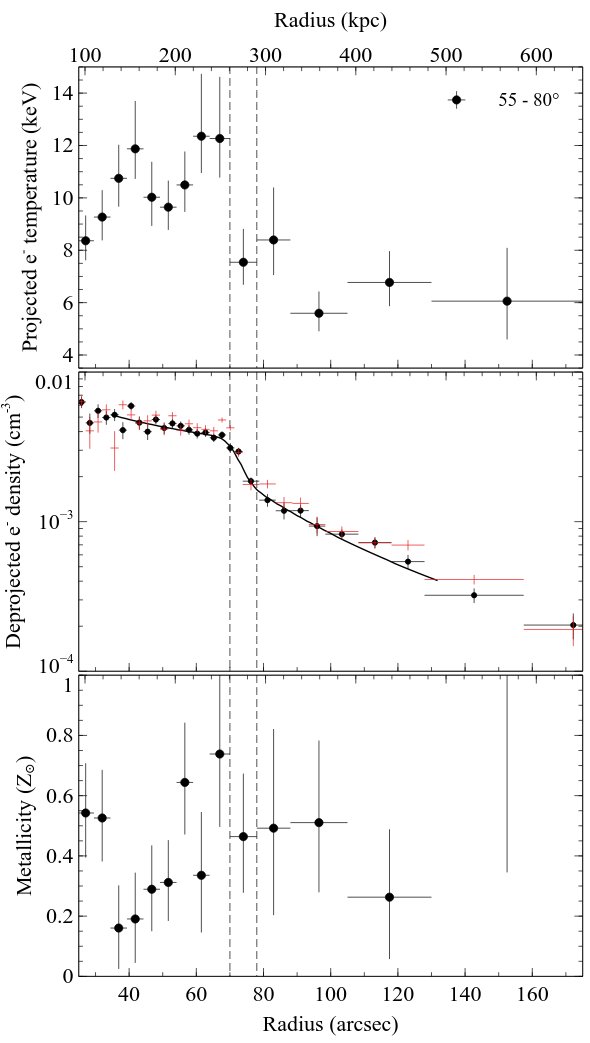
Figure 15: Projected temperature and metallicity profiles across the upstream shock front in the $55$–$80\deg$ sector (top and bottom panels). Deprojected electron density profile (middle panel) with the best-fit density jump model (solid black line) and the result from the $30$–$55\deg$ sector overlaid (red points). Vertical dashed lines approximate the full width of the density jump and guide the radial binning selected for the temperature profile.

Fig. 15 shows the projected temperature, metallicity and deprojected electron density profiles across the upstream shock front in the $55$–$80\deg$ sector. The temperature increases at the shock front from $6.0\pm 0.6\rm\;keV$ at large radius, to $8^{+2}_{-1}\rm\;keV$ roughly $50\rm\;kpc$ ahead of the shock front to $12.3^{+1.7}_{-1.0}\rm\;keV$ immediately behind the shock front. Although the increase ahead of the shock front appears only modestly significant, we show in section 6 that this increase in the preshock gas temperature explains the anomalously high postshock temperature, noted in our previous work (Russell et al. 2012). It is therefore likely that a ${\sim}2\rm\;keV$ increase in temperature occurs ${\sim}50\rm\;kpc$ ahead of the upstream shock front. From the density jump and the sound speed in the preshock gas $c_{\mathrm{s}}=1450^{+180}_{-90}\hbox{$\rm\;km\rm\;s^{-1}\,$}$, the shock velocity $v_{\mathrm{sh}}=2300^{+300}_{-200}\hbox{$\rm\;km\rm\;s^{-1}\,$}$. No significant increase in the density is seen at this location, and substructure in the surface brightness profiles has low significance (Fig. 14). Although the $30$–$55\deg$ sector shows a clear increase in the gas density in this region at ${\sim}300\rm\;kpc$, this is coincident with another primary cluster galaxy halo and therefore unrelated. Similar to the bow shock front, the metallicity is approximately constant at $0.39\pm 0.15\hbox{$\thinspace\mathrm{Z}_{\odot}$}$ in the preshock gas and $0.55\pm 0.12\hbox{$\thinspace\mathrm{Z}_{\odot}$}$ in the immediate postshock gas.

As noted earlier, hydrodynamical simulations of Abell 2146 have shown complex structure in the upstream shock (Chadayammuri et al. 2022; section 3). It is likely that a series of additional weaker shocks lie ahead of the upstream shock front. These structures could explain the observed temperature increase. Although the temperature increase is not clearly associated with a sharp density jump, surface brightness profiles for sectors across the centre of this shock show structure at low significance. This region is also projected onto the break up of the primary cluster’s core, which may obscure the shock density structure. If the temperature increase was due to a shock precursor, we would expect a comparable feature ahead of the bow shock front, which is not observed. We therefore consider a precursor origin to be less likely.

Following our analysis of the bow shock width above (section 5.1), we consider the width of the upstream shock front. For an upstream shock radius $R{\sim}267\pm 1\rm\;kpc$, width $\sigma_{\mathrm{sh}}=10.7\pm 0.3\rm\;kpc$ and shock velocity $v_{\mathrm{sh}}=2300^{+300}_{-200}\hbox{$\rm\;km\rm\;s^{-1}\,$}$, we estimate $\sigma_{\mathrm{turb}}=290\pm 30\hbox{$\rm\;km\rm\;s^{-1}\,$}$. The turbulent level is therefore similar ahead of both shock fronts. In this model, the upstream shock is narrower than the bow shock because it is younger. The upstream shock forms later during the merger, which is confirmed by hydrodynamical simulations (Chadayammuri et al. 2022).

The electron mean free path across the upstream shock is very similar to the bow shock at $\lambda_{\mathrm{e}}=15\pm 5\rm\;kpc$ (Fig. 12). The narrower width of the upstream shock relative to the mean free path strengthens our earlier conclusion that the shock fronts in Abell 2146 are collisionless and broadened in projection by turbulence in the preshock gas.

In summary: we fit a projected density jump model to surface brightness profiles extracted in narrow sectors across each shock. The model’s free parameters include the shock width and the density increase across the shock, which is used to calculate the Mach number. The bow shock Mach number $M=2.24\pm 0.09$. The angular dependence of the Mach number is much steeper than the expected $\mathrm{cos}{\theta}$ dependence. This is likely due to a break down in key assumptions of steady shock velocity and uniform preshock medium. The best-fit shock width of $\sigma_{\mathrm{sh}}=17\pm 1\rm\;kpc$ is significantly preferred over an unresolved width. A similar analysis of the upstream shock front finds $M=1.58\pm 0.05$ and $\sigma_{\mathrm{sh}}=10.7\pm 0.3\rm\;kpc$. The shocks appear too narrow to be collisional. Collisionless shocks are typically npc in width but will appear much broader in projection if their smooth shape is warped by turbulence in the preshock gas. We show that both shock widths are consistent with collisionless shocks propagating through a turbulent medium with $\sigma_{\mathrm{turb}}=290\pm 30\hbox{$\rm\;km\rm\;s^{-1}\,$}$. The upstream shock is narrower than the bow shock because it is younger. We also find a ${\sim}2\rm\;keV$ increase in temperature ${\sim}50\rm\;kpc$ ahead of the upstream shock front, which is likely due to additional weak shocks.

6 Electron-ion thermal equilibration behind shock fronts

Electron and ion heating by collisionless shocks remains an unsolved problem in shock physics. This problem has received much less attention than non-thermal particle acceleration (e.g. Ghavamian et al. 2013). The more massive ions are directly heated in the shock layer by plasma-wave interactions between the ions and the magnetic field. The electrons then subsequently thermally equilibrate with the shock-heated ions. However, the exact mechanism and timescale are unknown. Collisionless shocks occur over a wide range of scales in astrophysics from accretion shocks at the intersection of massive cosmic structure filaments to supernova remnants and solar wind shocks (e.g. Marcowith et al. 2016). Whilst the shock parameters differ, only in galaxy clusters are we able to map the large-scale equilibration processes in a single observation (see section 2) and avoid systematic errors from cross-calibrating observations in different wavebands.

6.1 Equilibration models

Following Markevitch (2006) and Russell et al. (2012) (see also Wang et al. 2018), we measured the temperature profiles across each shock front to estimate the timescale for the electrons and ions to return to thermal equilibrium. Fig. 16 shows the measured electron temperature across the bow shock in Abell 2146 for the sector $225$–$260\deg$. We note that an even more conservative sector selection from $235$–$255^{\circ}$ produces a consistent result. We compare the observed profile with two models for electron-ion thermal equilibration. The instant equilibration model assumes that the electrons rapidly equilibrate with the hotter ions over an unresolved distance. The electron temperature and the ion temperature jump at the shock front to the post-shock gas temperature given by the Rankine-Hugoniot shock jump conditions. The second model is the collisional equilibration model, which assumes an unresolved adiabatic increase in electron temperature,

$$T_{\mathrm{e,2}}=T_{\mathrm{e,1}}\left(\frac{n_{\mathrm{e,2}}}{n_{\mathrm{e,1}}}\right)^{\gamma-1}.$$ (3)

Charge neutrality ties the electron density to the ion density very rigidly so the electron density jumps at the ion shock. This adiabatic increase is followed by a slower equilibration via Coulomb collisions at a rate

$$\frac{\mathrm{d}T_{\mathrm{e}}}{\mathrm{d}t}=\frac{T_{\mathrm{i}}-T_{\mathrm{e}}}{t_{\mathrm{cc}}}.$$ (4)

$T_{\mathrm{e}}$ is the electron temperature, $T_{\mathrm{i}}$ is the ion temperature and $n_{\mathrm{e}}$ is the electron temperature. The subscripts 1 and 2 denote the preshock and postshock values, respectively. The Coulomb collisional timescale is given by

$$t_{\mathrm{cc}}=2.54\times 10^{8}\left(\frac{T_{\mathrm{e}}}{10^{8}\rm\;K}\right)^{3/2}\left(\frac{n_{\mathrm{e}}}{10^{-3}\hbox{$\rm\;cm^{-3}\,$}}\right)^{-1}\rm\;yr$$ (5)

(e.g. Wong & Sarazin 2009; Sarazin et al. 2016). The electron temperature as a function of time for the collisional model was determined analytically by integrating equation 4. The shock velocity in the postshock gas was used to determine the electron temperature as a function of distance.

To summarise: the observed preshock electron temperature was combined with the measured electron density jump to predict the postshock electron temperature under the assumptions of two different equilibration models. The collisional equilibration model assumes adiabatic compression of the electrons at the shock followed by equilibration on the collisional timescale. The instant equilibration model assumes an additional electron heating mechanism that rapidly heats the electrons over an unresolved distance. For details see Russell et al. (2012).

Both equilibration models were projected by calculating the emission measure of gas at each temperature along lines of sight through the cluster. The projection assumed the density model determined in section 5 and blurring to incorporate the shock width. By simulating spectra in xspec with the predicted emission measure distribution, we generated projected temperature profiles for each model. The input parameters for the equilibration models were the preshock temperature, the slopes and normalizations of each powerlaw, shock radius and width. We generated 1000 Monte Carlo simulations of these parameters using the realizations of the density model and drawing preshock temperature values from a Gaussian distribution based on the mean and uncertainty. The output equilibration models are the median output model profiles from this process.

6.2 Bow shock

Fig. 16 shows the projected electron temperature profile across the bow shock and the instant and collisional equilibration models. The instant equilibration model is a particularly poor fit to the observed temperature profile with $\chi^{2}=46.6$ for 4 degrees of freedom (the postshock datapoints). We conservatively exclude the datapoint closest to the subcluster’s cool core. Although not immediately apparent from the images and temperature map, this region may contain a low level of cooler stripped material. In addition, the simplifying assumptions of the density model breakdown with increasing distance behind the shock (see section 5). From the p-value of $2\times 10^{-9}$, the observed profile is inconsistent with the instant equilibration model at the $6\sigma$ level. A consistent result is obtained if the preshock temperature is included as a free parameter rather than assuming the observed value and corresponding uncertainty. We therefore rule out the instant equilibration model for the bow shock in Abell 2146.

The collisional equilibration model provides an improved fit to the observed temperature profile with $\chi^{2}=14.0$ for 4 degrees of freedom. Although the observed temperature ${>}100\rm\;kpc$ behind the shock appears low compared to the model predictions, this discrepancy is not particularly significant ($2.5\sigma$). Adiabatic expansion of the gas in the postshock region would lower the temperature. However, the postshock electron pressure agrees with the prediction from the shock jump conditions. The pressure is then constant or increasing from the shock front to the subcluster’s cool core. Adiabatic losses do not therefore appear significant over this distance.

Instead, it is likely that the low postshock temperature reflects the changing state of the preshock gas as the subcluster travels through the core of the primary cluster. The equilibration models for the postshock gas temperature are generated from the shock density jump and the preshock temperature, which are assumed constant. However, the hot atmosphere e.g. $100\rm\;kpc$ behind the shock was heated by the shock ${\sim}10^{8}\rm\;yr$ ago when the preshock conditions were likely different. The subcluster is travelling through the primary cluster’s core and the preshock conditions vary depending on the unknown, unperturbed temperature and density structure. Therefore, whilst the collisional equilibration model accurately predicts the immediate postshock temperature (Fig. 16), we expect increasing departures from this model with increasing distance behind the shock. An accurate prediction of the preshock conditions from the path of the subcluster through the primary is beyond the capabilities of our existing simple equilibration models and the hydrodynamical simulations of Abell 2146.

6.3 Comparison with other collisionless shocks

Analyses of cluster merger shock fronts in the Bullet cluster and Abell 520 concluded instant equilibration of the electrons and ions at the $2\sigma$ level (Markevitch 2006; Wang et al. 2018). However, an ALMA and ACA analysis of the Bullet cluster shock by Di Mascolo et al. (2019) found that a purely adiabatic electron temperature change (i.e. no additional electron heating) produced the best agreement between the thermal Sunyaev-Zeldovich and X-ray results. Although the shock properties for these three systems are broadly comparable, it is possible that they have different structure, which produces different rates of equilibration. In future, X-ray microcalorimeters will map electron and ion temperatures behind nearby shock fronts and increase the sample size for these equilibration measurements.

Electron heating in low Mach number cluster shocks with high $\beta$ (ratio of thermal to magnetic pressure) has been investigated with particle-in-cell (PIC) simulations (e.g. Caprioli & Spitkovsky 2014a, b; Guo et al. 2014, 2017, 2018; Ha et al. 2018; Xu et al. 2020). Guo et al. (2017), for example, found additional electron heating over adiabatic compression due to the growth of whistler waves. For the bowshock in Abell 2146, with $M=2.24\pm 0.09$ and preshock electron temperature $6.0\pm 0.6\rm\;keV$, their analytical model predicts this mechanism would heat the electrons by ${\sim}0.5\rm\;keV$ above adiabatic compression. Unfortunately, the existing data cannot distinguish such a modest increase in electron heating over the collisional model.

Observations of low Mach number heliospheric shocks have shown minimal electron heating beyond adiabatic compression (e.g. Thomsen et al. 1987; Schwartz et al. 1988; Hull et al. 2000; Masters et al. 2011). However, the measured electron distributions show significant deviations from Maxwellians and they found no conclusive evidence of the dependence of electron heating on shock parameters (Wilson et al. 2019a, b, 2020). For higher Mach numbers in supernova remnants, the shock transition is likely turbulent and disordered because plasma instabilities driven by the ions are typically reflected back upstream. Especially in regions where the shock normal is quasi-parallel to the background magnetic field (e.g. Caprioli et al. 2015). Self-consistent kinetic simulations show that both ions (Caprioli & Spitkovsky 2014a, b) and electrons (Park et al. 2015) are then heated non-adiabatically in the shock precursor. Evidence of electron collisionless heating in PIC simulations has been found also for oblique and quasi-perpendicular shocks (e.g. Matsumoto et al. 2015; Xu et al. 2020; Bohdan et al. 2020, and references therein).

In general, electron heating at collisionless shocks should exhibit a dependence on the shock velocity and Mach number. Rapid equilibration is fostered by the presence of upstream plasma instabilities driven by accelerated particles. The bowshock in Abell 2146 appears consistent with this picture with a low Mach number and minimal electron heating over that produced by adiabatic compression and collisional equilibration.

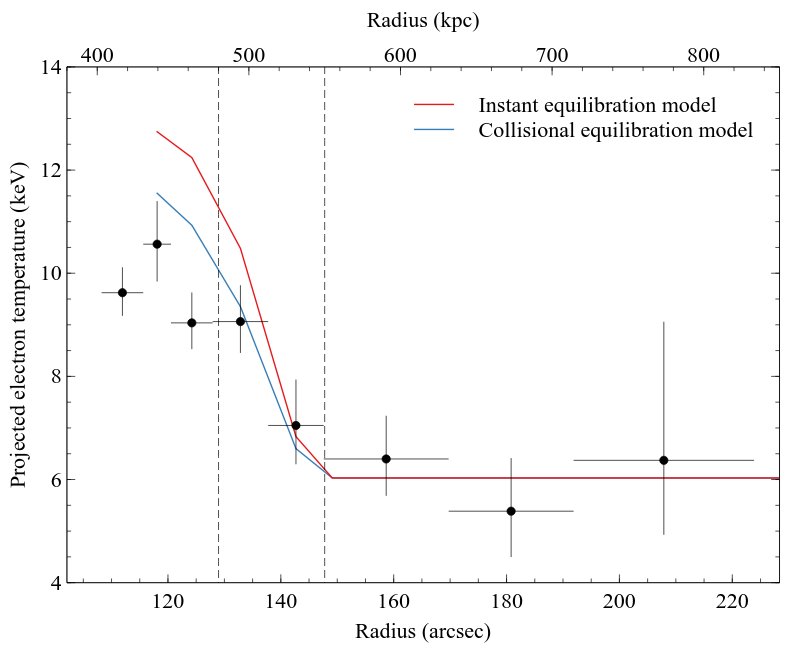
Figure 16: Projected temperature profile extracted in narrow (black points) and broad (white points) radial bins across the bow shock front (from Fig. 11) with best-fit models for collisional (blue) and instant equilibration (red) of the electrons and ions behind the shock.

6.4 Upstream shock

In principle, the upstream shock front could provide a second test of electron heating at cluster merger shocks. However, in practice, the complex temperature structure at the upstream shock and ram pressure stripping of the primary cluster’s galaxy atmospheres downstream prevents an unambiguous measurement. Fig. 15 shows the temperature increasing from $6.0\pm 0.6\rm\;keV$ at large radius to $8^{+2}_{-1}\rm\;keV$ at a distance of roughly $50\rm\;kpc$ ahead of the shock front. The projected density jump model shows that this increase clearly occurs before this narrow shock front. This temperature increase could not be identified in our earlier study of this merger. Based on a preshock temperature of ${\sim}6\rm\;keV$, Russell et al. (2012) found that the postshock gas temperature was above the expectation from the shock jump conditions and the equilibration models. Now using a preshock temperature of $8^{+2}_{-1}\rm\;keV$ we find that the postshock temperature is consistent (Fig. 17). Given the lower Mach number, the larger uncertainties on the preshock temperature and the complex temperature structure, the different equilibration models cannot be distinguished behind the upstream shock.

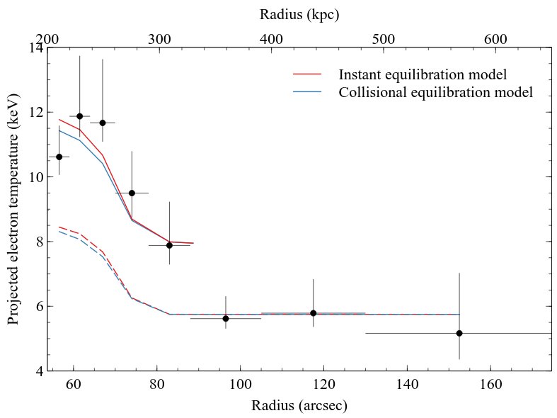
Figure 17: Projected temperature profile extracted in the $30$–$80^{\circ}$ sector across the upstream shock front (from Fig. 15). Illustrative models for collisional (blue) and instant (red) equilibration are shown for two different preshock temperatures: $6\rm\;keV$ (dashed lines) and $8\rm\;keV$ (solid lines).

7 Systematic uncertainties

Here we consider the impact of the key sources of systematic uncertainty on the best-fit density jump parameters and equilibration analysis for the bow shock. As discussed in section 2, measured spectral normalization appears on average a few per cent higher in the new datasets compared to the 2010 observations. This is likely due to the escalating contaminant correction. If the new datasets are ‘corrected’ for this offset to match the older observations, the powerlaw normalizations for the projected density jump model are systematically lower by $\sim 1\%$. This uncertainty is insignificant compared to the statistical uncertainties. All other parameters are unaffected. In addition to this calibration systematic, the X-ray spectral modelling makes a series of assumptions regarding the applicability of thermal plasma emission models (see discussion in section 4). In future, X-ray microcalorimeters will start to evaluate the systematic uncertainties related to these assumptions.

The new observations were taken over a wide range of roll angles so the shock fronts lie on a different part of the ccd in each dataset. The satellite’s roll angle measures rotation about the viewing axis, which is perpendicular to the ccd or detector plane. The roll angle varies over time to ensure the solar panels can always directly view the sun and to maintain preferred operating temperatures. Observations at different roll angles can be advantageous. It ensures that the results are less dependent on the calibration of chip non-uniformities. However, the shock fronts then lie at a range of distances up to $5\rm\;arcmin$ from the ACIS-I focal point. For surface brightness profiles in the $0.5-4\rm\;keV$ band, the majority of the photons have energies below $2\rm\;keV$. At these energies, 50 per cent of the photons will fall within a radius of $0.5\rm\;arcsec$ for an on-axis source and within $1.5\rm\;arcsec$ at $5\rm\;arcmin$ off-axis. Our analysis assumes an average of $1\rm\;arcsec$ PSF blurring, which is appropriate given the large number of observations spanning all roll angles. We tested blurring of $0.5\rm\;arcsec$ and $1.5\rm\;arcsec$ and found systematic differences in the shock width of $-0.2\rm\;kpc$ and $+0.2\rm\;kpc$, respectively. This would be a key systematic for much narrower shocks but is not particularly significant here.

Galaxy dynamical measurements indicate that the merger axis is only $13-19^{\circ}$ from the plane of the sky (Canning et al. 2012; White et al. 2015). The tightest constraint comes from the small line of sight velocity difference between the BCGs, which most accurately trace the centres of the respective dark matter halos. Whilst hydrodynamical simulations of Abell 2146 indicate an inclination angle up to $30^{\circ}$ from the plane of the sky, this analysis is based on matching the X-ray morphology and uncertainties are expected to be significantly larger (Chadayammuri et al. 2022). The strongest constraint in these simulations is from the standoff distance, between the bow shock and the leading edge of the subcluster core, which favours inclination angles of $15-30^{\circ}$. Chadayammuri et al. (2022) show minimal differences between temperature profiles for inclination angles $<20^{\circ}$. Inclination effects are therefore expected to be minimal.

We tested the impact of a systematic increase or decrease in the background by $1\sigma$. This had a neligible impact on the projected density model parameters but resulted in a systematic variation in the measured preshock temperature of $\pm 0.3\rm\;keV$. The increase in cluster surface brightness by roughly an order of magnitude from the preshock to postshock gas ensured a minimal effect on the measured postshock temperatures. The equilibration analysis was repeated with these systematically shifted temperature profiles and the corresponding projected density model parameters. The single fluid model is ruled out at $5\sigma$ and $7\sigma$ for a systematic decrease or increase in the background by $1\sigma$, respectively.

The dominant source of systematic uncertainty is the changing state of the preshock gas as the subcluster travels through the core of the primary cluster. The projected density jump and equilibration models assume a constant shock density jump and preshock temperature. However, the hot atmosphere at large distances behind the shock was heated by the shock ${\sim}10^{8}\rm\;yr$ ago, or roughly around core passage. The preshock conditions were likely different. Therefore, whilst our models should accurately predict the immediate postshock conditions, the systematic uncertainties increase with distance behind the shock. An accurate prediction of the preshock conditions from the path of the subcluster through the primary is beyond the capabilities of our existing simple equilibration models and the hydrodynamical simulations of Abell 2146.

8 Conclusions

The galaxy cluster merger Abell 2146 features two huge shock fronts each ${\sim}500\rm\;kpc$ in length. The bow shock, with $M=2.24\pm 0.09$, lies ${\sim}150\rm\;kpc$ ahead of the subcluster’s core. The upstream shock front, $M=1.56\pm 0.05$, lies on the far side of the primary cluster’s centre and propagates in the opposite direction. The new $2\rm\;Ms$ Chandra observation of this cluster is the deepest of merger shock fronts and represents a legacy dataset for studying their structure.

For the first time, we resolve and measure the width of merger shocks. The bow shock width is $17\pm 1\rm\;kpc$ and the upstream shock is significantly narrower at $10.7\pm 0.3\rm\;kpc$. The widths are comparable to the electron mean free path across each shock at $11\pm 2\rm\;kpc$ and $15\pm 5\rm\;kpc$ for the bow and upstream shocks, respectively. Collisional shock widths should be a few times the mean free path. Modest aberrations in the shock shape across the wide sector analysed further broaden the shock when seen in projection. These shocks appear too narrow to be collisional. Instead, they may be narrow collisionless shock fronts that appear broader because their smooth shape is warped by local gas motions. The widths of both shock fronts are consistent with local gas motions of $290\pm 30\hbox{$\rm\;km\rm\;s^{-1}\,$}$, which have modulated the shock speed. The upstream shock is then expected to be narrower than the bow shock, as observed, because it forms later in the merger. This measurement of turbulence at radii of a few hundred kpc is consistent with the turbulent level measured in cluster cores at radii of a few tens of kpc. This implies a slow increase in turbulent velocity with radius.

By mapping the electron temperature structure behind the bow shock, we measure the timescale for the electrons and ions to return to thermal equilibrium. For a collisionless shock front, plasma-wave interactions between the ions and the magnetic field will heat the massive ions in the narrow shock layer. The electrons then subsequently equilibrate with the hotter ions. We rule out rapid thermal equilibration, over an unresolved distance, at the $6\sigma$ level. Instead, the observed electron temperature structure supports adiabatic compression of the electrons in the shock layer followed by equilibration on the collisional timescale over ${>}150\rm\;kpc$.

Our results for Abell 2146 are expected to be valid for collisionless shocks with similar parameters in other environments and support the existing picture from the solar wind and supernova remnants. We rule out strong electron heating but cannot distinguish more modest electron heating over that due to adiabatic compression and collisional equilibration. The upstream shock is consistent with these findings but has a more complex structure with a ${\sim}2\rm\;keV$ increase in electron temperature ${\sim}50\rm\;kpc$ ahead of the shock’s density jump. Hydrodynamical simulations of Abell 2146 show this is likely due to a series of additional weaker shocks, which occur ahead of the upstream shock. These structures are projected onto the break up of the primary cluster’s core, which likely obscures corresponding density increases.

In future, X-ray microcalorimeters will resolve thermal line broadening and measure both the ion and electron temperatures behind nearby shock fronts. With a larger sample, we will determine if the electron heating rate differs between systems, whether it depends on shock parameters and search for shock precursors and regions of non-equilibrium ionization.

Table 1:

Date	Obs. ID	Aim point	Exposure	Cleaned	Date	Obs. ID	Aim point	Exposure	Cleaned
			(ks)	(ks)				(ks)	(ks)
2010 August 10	13020	I0	41.5	41.5	2019 May 19	22225	I3	36.4	36.4
2010 August 12	13021	I0	48.4	48.4	2019 May 20	20915	I3	36.6	36.6
2010 August 19	13023	I1	27.7	27.7	2019 May 22	22228	I3	42.4	42.4
2010 August 20	12247	I1	65.2	65.2	2019 May 27	20919	I3	16.8	16.8
2010 September 8	12245	I2	48.3	48.3	2019 May 27	22235	I3	15.4	15.4
2010 September 10	13120	I2	49.4	49.4	2019 May 28	22236	I3	35.2	35.2
2010 October 4	12246	I3	47.4	47.2	2019 May 29	22237	I3	28.7	28.7
2010 October 10	13138	I3	49.4	48.6	2019 May 31	22238	I3	29.7	29.7
2018 June 5	20555	I3	48.4	48.4	2019 June 3	22030	I3	34.6	34.6
2018 June 8	21101	I3	34.6	34.6	2019 June 5	22241	I3	54.3	54.3
2018 July 10	20556	I3	35.0	35.0	2019 June 7	22242	I3	20.7	20.7
2018 July 17	20557	I3	49.4	49.4	2019 June 9	22243	I3	28.7	28.7
2018 July 18	21130	I3	32.6	32.6	2019 June 10	20560	I3	37.6	37.6
2018 July 24	20912	I3	34.2	34.2	2019 June 13	22253	I3	24.7	24.7
2018 July 27	21135	I3	21.8	21.8	2019 June 16	22254	I3	19.8	19.8
2018 July 28	21136	I3	21.8	20.7	2019 June 16	20562	I3	33.6	33.6
2018 September 7	20913	I3	10.8	10.8	2019 June 19	22258	I3	22.8	22.8
2018 September 8	21733	I3	56.3	56.3	2019 June 21	22259	I3	19.8	19.8
2018 December 1	21970	I3	13.0	13.0	2019 June 22	22260	I3	25.7	25.7
2018 December 2	20917	I3	21.8	21.8	2019 June 24	20561	I3	31.6	31.6
2018 December 5	20923	I3	17.8	17.8	2019 June 26	22262	I3	13.1	13.1
2018 December 6	21996	I3	14.0	14.0	2019 June 28	22263	I3	44.7	44.7
2018 December 15	20553	I3	19.8	19.8	2019 June 29	22264	I3	21.8	21.8
2018 December 20	22011	I3	19.8	19.8	2019 June 30	22265	I3	32.3	32.3
2018 December 25	20914	I3	20.1	20.1	2019 July 15	22200	I3	41.5	41.5
2018 December 26	22028	I3	23.8	23.8	2019 July 22	20563	I3	22.8	22.8
2019 January 5	22029	I3	32.6	32.6	2019 July 31	20918	I3	22.8	22.8
2019 March 2	20921	I3	19.8	16.1	2019 August 3	22678	I3	39.5	39.5
2019 March 2	22129	I3	29.7	29.7	2019 August 5	20559	I3	40.1	40.1
2019 March 10	22097	I3	33.6	30.1	2019 August 11	22286	I3	16.8	16.8
2019 March 14	20554	I3	34.8	34.8	2019 August 18	22093	I3	24.7	24.7
2019 April 6	20916	I3	39.5	39.5	2019 August 20	22079	I3	17.6	17.6
2019 April 7	20558	I3	27.4	27.4	2019 August 21	22731	I3	39.5	39.5
2019 April 24	21674	I3	21.8	16.9	2019 August 22	22732	I3	28.7	28.7
2019 May 9	20920	I3	20.9	20.9	2019 August 23	22733	I3	44.5	44.5
2019 May 12	22217	I3	17.8	17.8	2019 August 24	22734	I3	34.6	34.6
2019 May 15	20552	I3	39.5	39.5	2019 August 30	20922	I3	19.0	19.0
2019 May 17	22224	I3	22.8	22.8

Data availability

The Chandra data described in this work are available in the Chandra data archive (https://cxc.harvard.edu/cda/). Processed data products detailed in this paper will be made available on reasonable request to the author.

References

- Akahori & Yoshikawa (2010) Akahori T., Yoshikawa K., 2010, PASJ, \hrefhttp://adsabs.harvard.edu/abs/2010PASJ…62..335A 62, 335
- Akahori & Yoshikawa (2012) Akahori T., Yoshikawa K., 2012, \hrefhttp://dx.doi.org/10.1093/pasj/64.1.12 PASJ, \hrefhttps://ui.adsabs.harvard.edu/abs/2012PASJ…64…12A 64, 12
- Anders & Grevesse (1989) Anders E., Grevesse N., 1989, \hrefhttp://dx.doi.org/10.1016/0016-7037(89)90286-X Geochim. Cosmochim. Acta, \hrefhttp://adsabs.harvard.edu/abs/1989GeCoA..53..197A 53, 197
- Arnaud (1996) Arnaud K. A., 1996, in Jacoby G. H., Barnes J., eds, Astronomical Society of the Pacific Conference Series Vol. 101, Astronomical Data Analysis Software and Systems V. pp 17–+
- Bohdan et al. (2020) Bohdan A., Pohl M., Niemiec J., Morris P. J., Matsumoto Y., Amano T., Hoshino M., 2020, \hrefhttp://dx.doi.org/10.3847/1538-4357/abbc19 ApJ, \hrefhttps://ui.adsabs.harvard.edu/abs/2020ApJ…904…12B 904, 12
- Böhringer & Werner (2010) Böhringer H., Werner N., 2010, \hrefhttp://dx.doi.org/10.1007/s00159-009-0023-3 A&A Rev., \hrefhttps://ui.adsabs.harvard.edu/abs/2010A&ARv..18..127B 18, 127
- Böhringer et al. (2000) Böhringer H., et al., 2000, \hrefhttp://dx.doi.org/10.1086/313427 ApJS, \hrefhttp://adsabs.harvard.edu/abs/2000ApJS..129..435B 129, 435
- Canning et al. (2012) Canning R. E. A., et al., 2012, \hrefhttp://dx.doi.org/10.1111/j.1365-2966.2011.20116.x MNRAS, \hrefhttps://ui.adsabs.harvard.edu/abs/2012MNRAS.420.2956C 420, 2956
- Caprioli & Spitkovsky (2014a) Caprioli D., Spitkovsky A., 2014a, \hrefhttp://dx.doi.org/10.1088/0004-637X/783/2/91 ApJ, \hrefhttps://ui.adsabs.harvard.edu/abs/2014ApJ…783…91C 783, 91
- Caprioli & Spitkovsky (2014b) Caprioli D., Spitkovsky A., 2014b, \hrefhttp://dx.doi.org/10.1088/0004-637X/794/1/46 ApJ, \hrefhttps://ui.adsabs.harvard.edu/abs/2014ApJ…794…46C 794, 46
- Caprioli et al. (2015) Caprioli D., Pop A.-R., Spitkovsky A., 2015, \hrefhttp://dx.doi.org/10.1088/2041-8205/798/2/L28 ApJ, \hrefhttps://ui.adsabs.harvard.edu/abs/2015ApJ…798L..28C 798, L28
- Cash (1979) Cash W., 1979, \hrefhttp://dx.doi.org/10.1086/156922 ApJ, \hrefhttp://adsabs.harvard.edu/abs/1979ApJ…228..939C 228, 939
- Chadayammuri et al. (2022) Chadayammuri U., ZuHone J., Nulsen P., Nagai D., Felix S., Andrade-Santos F., King L., Russell H., 2022, \hrefhttp://dx.doi.org/10.1093/mnras/stab2629 MNRAS, \hrefhttps://ui.adsabs.harvard.edu/abs/2022MNRAS.509.1201C 509, 1201
- Churazov et al. (2016) Churazov E., Arevalo P., Forman W., Jones C., Schekochihin A., Vikhlinin A., Zhuravleva I., 2016, \hrefhttp://dx.doi.org/10.1093/mnras/stw2044 MNRAS, \hrefhttps://ui.adsabs.harvard.edu/abs/2016MNRAS.463.1057C 463, 1057
- Clowe et al. (2006) Clowe D., Bradač M., Gonzalez A. H., Markevitch M., Randall S. W., Jones C., Zaritsky D., 2006, \hrefhttp://dx.doi.org/10.1086/508162 ApJ, \hrefhttp://adsabs.harvard.edu/abs/2006ApJ…648L.109C 648, L109
- Di Mascolo et al. (2019) Di Mascolo L., et al., 2019, \hrefhttp://dx.doi.org/10.1051/0004-6361/201936184 A&A, \hrefhttps://ui.adsabs.harvard.edu/abs/2019A&A…628A.100D 628, A100
- Ghavamian et al. (2013) Ghavamian P., Schwartz S. J., Mitchell J., Masters A., Laming J. M., 2013, \hrefhttp://dx.doi.org/10.1007/s11214-013-9999-0 Space Sci. Rev., \hrefhttps://ui.adsabs.harvard.edu/abs/2013SSRv..178..633G 178, 633
- Guo et al. (2014) Guo X., Sironi L., Narayan R., 2014, \hrefhttp://dx.doi.org/10.1088/0004-637X/794/2/153 ApJ, \hrefhttps://ui.adsabs.harvard.edu/abs/2014ApJ…794..153G 794, 153
- Guo et al. (2017) Guo X., Sironi L., Narayan R., 2017, \hrefhttp://dx.doi.org/10.3847/1538-4357/aa9b82 ApJ, \hrefhttps://ui.adsabs.harvard.edu/abs/2017ApJ…851..134G 851, 134
- Guo et al. (2018) Guo X., Sironi L., Narayan R., 2018, \hrefhttp://dx.doi.org/10.3847/1538-4357/aab6ad ApJ, \hrefhttps://ui.adsabs.harvard.edu/abs/2018ApJ…858…95G 858, 95
- Ha et al. (2018) Ha J.-H., Ryu D., Kang H., van Marle A. J., 2018, \hrefhttp://dx.doi.org/10.3847/1538-4357/aad634 ApJ, \hrefhttps://ui.adsabs.harvard.edu/abs/2018ApJ…864..105H 864, 105
- Hitomi Collaboration et al. (2016) Hitomi Collaboration et al., 2016, \hrefhttp://dx.doi.org/10.1038/nature18627 Nat, \hrefhttps://ui.adsabs.harvard.edu/abs/2016Natur.535..117H 535, 117
- Hull et al. (2000) Hull A. J., Scudder J. D., Fitzenreiter R. J., Ogilvie K. W., Newbury J. A., Russell C. T., 2000, \hrefhttp://dx.doi.org/10.1029/2000JA900049 J. Geophys. Res., \hrefhttps://ui.adsabs.harvard.edu/abs/2000JGR…10520957H 105, 20957
- Kalberla et al. (2005) Kalberla P. M. W., Burton W. B., Hartmann D., Arnal E. M., Bajaja E., Morras R., Pöppel W. G. L., 2005, \hrefhttp://dx.doi.org/10.1051/0004-6361:20041864 A&A, \hrefhttp://adsabs.harvard.edu/abs/2005A%26A…440..775K 440, 775
- King et al. (2016) King L. J., et al., 2016, \hrefhttp://dx.doi.org/10.1093/mnras/stw507 MNRAS, \hrefhttps://ui.adsabs.harvard.edu/abs/2016MNRAS.459..517K 459, 517
- Marcowith et al. (2016) Marcowith A., et al., 2016, \hrefhttp://dx.doi.org/10.1088/0034-4885/79/4/046901 Reports on Progress in Physics, \hrefhttps://ui.adsabs.harvard.edu/abs/2016RPPh…79d6901M 79, 046901
- Markevitch (2006) Markevitch M., 2006, in A. Wilson ed., ESA Special Publication Vol. 604, The X-ray Universe 2005. pp 723–+
- Markevitch & Vikhlinin (2007) Markevitch M., Vikhlinin A., 2007, \hrefhttp://dx.doi.org/10.1016/j.physrep.2007.01.001 Phys. Rep., \hrefhttp://adsabs.harvard.edu/abs/2007PhR…443….1M 443, 1
- Markevitch et al. (2005) Markevitch M., Govoni F., Brunetti G., Jerius D., 2005, \hrefhttp://dx.doi.org/10.1086/430695 ApJ, \hrefhttp://adsabs.harvard.edu/abs/2005ApJ…627..733M 627, 733
- Masters et al. (2011) Masters A., et al., 2011, \hrefhttp://dx.doi.org/10.1029/2011JA016941 Journal of Geophysical Research (Space Physics), \hrefhttps://ui.adsabs.harvard.edu/abs/2011JGRA..11610107M 116, A10107
- Matsumoto et al. (2015) Matsumoto Y., Amano T., Kato T. N., Hoshino M., 2015, \hrefhttp://dx.doi.org/10.1126/science.1260168 Science, \hrefhttps://ui.adsabs.harvard.edu/abs/2015Sci…347..974M 347, 974
- Nandra et al. (2013) Nandra K., et al., 2013, arXiv e-prints, \hrefhttps://ui.adsabs.harvard.edu/abs/2013arXiv1306.2307N p. arXiv:1306.2307
- Nulsen et al. (2013) Nulsen P. E. J., et al., 2013, \hrefhttp://dx.doi.org/10.1088/0004-637X/775/2/117 ApJ, \hrefhttps://ui.adsabs.harvard.edu/abs/2013ApJ…775..117N 775, 117
- Park et al. (2015) Park J., Caprioli D., Spitkovsky A., 2015, \hrefhttp://dx.doi.org/10.1103/PhysRevLett.114.085003 PhRvL, \hrefhttps://ui.adsabs.harvard.edu/abs/2015PhRvL.114h5003P 114, 085003
- Russell et al. (2008) Russell H. R., Sanders J. S., Fabian A. C., 2008, \hrefhttp://dx.doi.org/10.1111/j.1365-2966.2008.13823.x MNRAS, \hrefhttp://adsabs.harvard.edu/abs/2008MNRAS.390.1207R 390, 1207
- Russell et al. (2010) Russell H. R., Sanders J. S., Fabian A. C., Baum S. A., Donahue M., Edge A. C., McNamara B. R., O’Dea C. P., 2010, \hrefhttp://dx.doi.org/10.1111/j.1365-2966.2010.16822.x MNRAS, \hrefhttp://adsabs.harvard.edu/abs/2010MNRAS.406.1721R 406, 1721
- Russell et al. (2012) Russell H. R., et al., 2012, \hrefhttp://dx.doi.org/10.1111/j.1365-2966.2012.20808.x MNRAS, \hrefhttps://ui.adsabs.harvard.edu/abs/2012MNRAS.423..236R 423, 236
- Sanders (2006) Sanders J. S., 2006, \hrefhttp://dx.doi.org/10.1111/j.1365-2966.2006.10716.x MNRAS, \hrefhttp://adsabs.harvard.edu/abs/2006MNRAS.371..829S 371, 829
- Sanders & Fabian (2007) Sanders J. S., Fabian A. C., 2007, \hrefhttp://dx.doi.org/10.1111/j.1365-2966.2007.12347.x MNRAS, \hrefhttp://adsabs.harvard.edu/abs/2007MNRAS.381.1381S 381, 1381
- Sanders et al. (2011) Sanders J. S., Fabian A. C., Smith R. K., 2011, \hrefhttp://dx.doi.org/10.1111/j.1365-2966.2010.17561.x MNRAS, \hrefhttps://ui.adsabs.harvard.edu/abs/2011MNRAS.410.1797S 410, 1797
- Sanders et al. (2014) Sanders J. S., Fabian A. C., Sun M., Churazov E., Simionescu A., Walker S. A., Werner N., 2014, \hrefhttp://dx.doi.org/10.1093/mnras/stu092 MNRAS, \hrefhttps://ui.adsabs.harvard.edu/abs/2014MNRAS.439.1182S 439, 1182
- Sanders et al. (2021) Sanders J. S., et al., 2021, arXiv e-prints, \hrefhttps://ui.adsabs.harvard.edu/abs/2021arXiv210614534S p. arXiv:2106.14534
- Sarazin (2002) Sarazin C. L., 2002, in Feretti L., Gioia I. M., Giovannini G., eds, Astrophysics and Space Science Library Vol. 272, Merging Processes in Galaxy Clusters. pp 1–38 (\hrefhttp://arxiv.org/abs/astro-ph/0105418 arXiv:astro-ph/0105418), \hrefhttp://dx.doi.org/10.1007/0-306-48096-4_1 doi:10.1007/0-306-48096-4_1
- Sarazin et al. (2016) Sarazin C. L., Finoguenov A., Wik D. R., Clarke T. E., 2016, arXiv e-prints, \hrefhttps://ui.adsabs.harvard.edu/abs/2016arXiv160607433S p. arXiv:1606.07433
- Schwartz et al. (1988) Schwartz S. J., Thomsen M. F., Bame S. J., Stansberry J., 1988, \hrefhttp://dx.doi.org/10.1029/JA093iA11p12923 J. Geophys. Res., \hrefhttp://adsabs.harvard.edu/abs/1988JGR….9312923S 931, 12923
- Smith et al. (2001) Smith R. K., Brickhouse N. S., Liedahl D. A., Raymond J. C., 2001, \hrefhttp://dx.doi.org/10.1086/322992 ApJ, \hrefhttps://ui.adsabs.harvard.edu/abs/2001ApJ…556L..91S 556, L91
- Spitzer (1956) Spitzer L., 1956, Physics of Fully Ionized Gases
- Struble & Rood (1999) Struble M. F., Rood H. J., 1999, \hrefhttp://dx.doi.org/10.1086/313274 ApJS, \hrefhttp://adsabs.harvard.edu/abs/1999ApJS..125…35S 125, 35
- Thomsen et al. (1987) Thomsen M. F., Mellott M. M., Stansberry J. A., Bame S. J., Gosling J. T., Russell C. T., 1987, \hrefhttp://dx.doi.org/10.1029/JA092iA09p10119 J. Geophys. Res., \hrefhttps://ui.adsabs.harvard.edu/abs/1987JGR….9210119T 92, 10119
- Treumann (2009) Treumann R. A., 2009, \hrefhttp://dx.doi.org/10.1007/s00159-009-0024-2 A&A Rev., \hrefhttps://ui.adsabs.harvard.edu/abs/2009A&ARv..17..409T 17, 409
- Vikhlinin et al. (2005) Vikhlinin A., Markevitch M., Murray S. S., Jones C., Forman W., Van Speybroeck L., 2005, \hrefhttp://dx.doi.org/10.1086/431142 ApJ, \hrefhttps://ui.adsabs.harvard.edu/abs/2005ApJ…628..655V 628, 655
- Wang et al. (2018) Wang Q. H. S., Giacintucci S., Markevitch M., 2018, \hrefhttp://dx.doi.org/10.3847/1538-4357/aab2aa ApJ, \hrefhttps://ui.adsabs.harvard.edu/abs/2018ApJ…856..162W 856, 162
- White et al. (2015) White J. A., et al., 2015, \hrefhttp://dx.doi.org/10.1093/mnras/stv1831 MNRAS, \hrefhttps://ui.adsabs.harvard.edu/abs/2015MNRAS.453.2718W 453, 2718
- Wilson et al. (2019a) Wilson Lynn B. I., et al., 2019a, \hrefhttp://dx.doi.org/10.3847/1538-4365/ab22bd ApJS, \hrefhttps://ui.adsabs.harvard.edu/abs/2019ApJS..243….8W 243, 8
- Wilson et al. (2019b) Wilson Lynn B. I., et al., 2019b, \hrefhttp://dx.doi.org/10.3847/1538-4365/ab5445 ApJS, \hrefhttps://ui.adsabs.harvard.edu/abs/2019ApJS..245…24W 245, 24
- Wilson et al. (2020) Wilson Lynn B. I., et al., 2020, \hrefhttp://dx.doi.org/10.3847/1538-4357/ab7d39 ApJ, \hrefhttps://ui.adsabs.harvard.edu/abs/2020ApJ…893…22W 893, 22
- Wong & Sarazin (2009) Wong K.-W., Sarazin C. L., 2009, \hrefhttp://dx.doi.org/10.1088/0004-637X/707/2/1141 ApJ, \hrefhttps://ui.adsabs.harvard.edu/abs/2009ApJ…707.1141W 707, 1141
- Wong et al. (2011) Wong K.-W., Sarazin C. L., Ji L., 2011, \hrefhttp://dx.doi.org/10.1088/0004-637X/727/2/126 ApJ, \hrefhttp://adsabs.harvard.edu/abs/2011ApJ…727..126W 727, 126
- Xu et al. (2020) Xu R., Spitkovsky A., Caprioli D., 2020, \hrefhttp://dx.doi.org/10.3847/2041-8213/aba11e ApJ, \hrefhttps://ui.adsabs.harvard.edu/abs/2020ApJ…897L..41X 897, L41
- Zhang et al. (2019) Zhang C., Churazov E., Forman W. R., Jones C., 2019, \hrefhttp://dx.doi.org/10.1093/mnras/sty2501 MNRAS, \hrefhttps://ui.adsabs.harvard.edu/abs/2019MNRAS.482…20Z 482, 20
- van Weeren et al. (2019) van Weeren R. J., de Gasperin F., Akamatsu H., Brüggen M., Feretti L., Kang H., Stroe A., Zandanel F., 2019, \hrefhttp://dx.doi.org/10.1007/s11214-019-0584-z Space Sci. Rev., \hrefhttps://ui.adsabs.harvard.edu/abs/2019SSRv..215…16V 215, 16