Numerical Regge pole analysis of resonance structures in state-to-state reactive differential cross sections

Abstract

This is the third (and the last) code in a collection of three programs [Sokolovski et al (2011), Akhmatskaya et al (2014)] dedicated to the analysis of numerical data, obtained in an accurate simulation of an atom-diatom chemical reaction. Our purpose is to provide a detailed description of a FORTRAN code for complex angular momentum (CAM) analysis of the resonance effects in reactive angular scattering [for CAM analysis of integral reactive cross sections see [Akhmatskaya et al (2014)]. The code evaluates the contributions of a Regge trajectory (or trajectories) to a differential cross section in a specified range of energies. The contribution is computed with the help of the methods described in [Dobbyn et al (2007), Sokolovski and Msezane (2004), Sokolovski et al (2007)]. Regge pole positions and residues are obtained by analytically continuing $S$-matrix element, calculated numerically for the physical integer values of the total angular momentum, into the complex angular momentum plane using the PADE_II program [Sokolovski et al (2011)]. The code represents a reactive scattering amplitude as a sum of the components corresponding to a rapid ”direct” exchange of the atom, and the various scenarios in which the reactants form long-lived intermediate complexes, able to complete several rotations before breaking up into products. The package has been successfully tested on the representative models, as well as the F + H₂$\to$ HF+H benchmark reaction. Several detailed examples are given in the text.

PACS:34.50.Lf,34.50.Pi

PROGRAM SUMMARY

Manuscript Title: Numerical Regge pole analysis of resonance structures in reactive state-to-state differential cross sections.
Authors: E. Akhmatskaya, D. Sokolovski,
Program Title: DCS_Regge
Journal Reference:
Catalogue identifier:
Licensing provisions: Free software license
Programming language: FORTRAN 90
Computer: Any computer equipped with a FORTRAN 90 compiler
Operating system: UNIX, LINUX
RAM: 256 Mb
Has the code been vectorised or parallelised: no
Number of processors used: one
Supplementary material: PADE_II, MPFUN and QUADPACK packages, validation suites, script files, input files, readme files, Installation and User Guide
Keywords: Atomic and molecular collisions, reactive angular distributions, resonances, S-matrix; Padé approximation; Regge poles.
PACS: 34.50.Lf,34.50.Pi
Classification: Molecular Collisions
External routines/libraries: none
CPC Program Library subprograms used: N/A
Nature of problem:
The package extracts the positions and residues of resonance poles from numerical scattering data supplied by the user. This information is then used for the analysis of resonance structures observed in reactive differential cross sections.
Solution method:
The $S$-matrix element is analytically continued in the complex plane of either energy or angular momentum with the help of Padé approximation of type II. Resonance Regge trajectories are identified and their contributions to a differential cross section are evaluated at different angles and energies.
Restrictions:
None.
Unusual features:
Use of multiple precision $MPFUN$ package.
Additional comments: none
Running time:
from several minutes to hours depending on the number of energies involved, the precision level chosen and the number of iterations performed.
References:

• D. Sokolovski, E. Akhmatskaya and S. K. Sen, Comp. Phys. Comm. A, 182 (2011) 448.

• E. Akhmatskaya, D. Sokolovski, and C. Echeverría-Arrondo, Comp. Phys. Comm. A, 185 (2014) 2127.

• A.J. Dobbyn, P. McCabe, J.N.L. Connor and J.F. Castillo, Phys. Chem. Chem. Phys., 1 (1999) 1115.

• D. Sokolovski and A.Z. Msezane, Phys. Rev. A 70, (2004) 032710.

• D. Sokolovski, D. De Fazio, S. Cavalli and V. Aquilanti, Phys. Chem. Chem. Phys., 9 (2007) 5664.

LONG WRITE-UP

1 Introduction

In the last fifteen years the progress in crossed beams experimental techniques has been matched by the development of state-of-the-art computer codes capable of modelling atom-diatom elastic, inelastic and reactive differential and integral cross sections [1]- [10]. The differential cross sections (DCS), accessible to measurements in crossed beams, are often structured, and so offer a large amount of useful information about details of the collision or reaction mechanism. This information needs to be extracted and analysed, which often presents a challenging task. One distinguishes two main types of collisions: in a direct collision the partners depart soon after the first encounter, while in a resonance collision they form an intermediate complex (quasi-molecule), able to complete several rotations, before breaking up into products. The resonance pathways may become important or even dominant at low collision energies. For this reason, accurate modelling and understanding of resonance effects gain importance in such fields as cold atom physics and chemistry of the early universe.
Once the high quality scattered matrix is obtained numerically, one needs to understand the physics of the reaction, often not revealed until an additional analysis is carried out. In particular, resonances invariably leave their signatures on the differential state-to-state cross sections, as the rotation of the intermediate complex can carry the collision partners into the angular regions not probed by the direct mechanism. By a general rule of quantum mechanics, scenarios leading to the same outcome (in this case the same scattering angle) interfere, and complex interference patterns can be produced in the reactive DCS. In this paper we propose and describe software for the analysis of such resonance patterns. Relevant information on the Regge poles can be found in Refs.[11]-[16]. Some applications of the poles to the angular scattering and integral cross sections are discussed in Refs.[17]-[50]. For a description of the type-II Padé approximation, used by the software, the reader is referred to Refs.[51],[53].

2 Background and theory

We start with a brief review of the concepts and techniques required for our analysis.

2.1 Reactive differential cross-sections

For an atom-diatom reaction $A+BC\to AB+C$, a state-to-state differential cross section (DCS), also called an angular distribution, gives the number of products, scattered at a given energy $E$ into a unit solid angle around a direction $\theta_{R}$, per unit time, per unit solid angle, for unit incoming flux of the reactants. In the entire-of-mass frame, $\theta_{R}$ is the angle between the initial velocity of the atom $A$ and that of a newly formed molecule $AB$. The states of the molecule ($BC$ before and $AB$ after the reaction has taken place) is conveniently described by the vibrational ($v$), rotational ($j$), and helicity ($\Omega$ = projection of $j$ onto the final atom-diatom velocity) quantum numbers, and the cross section is obtained as an absolute square of a scattering amplitude

$$\sigma_{\nu^{\prime}\leftarrow\nu}(\theta_{R},E)=|f_{\nu^{\prime}\leftarrow\nu}(\theta_{R},E)|^{2},\quad\nu=(v,j,\Omega).$$ (1)

The scattering amplitude is given by a partial wave sum (PWS)

$$f_{\nu^{\prime}\leftarrow\nu}(\theta_{R},E)=(ik_{\nu})^{-1}\sum_{J=J_{min}}^{\infty}(J+1/2)S^{J}_{\nu{{}^{\prime}}\leftarrow\nu}d^{J}_{\Omega^{\prime}\Omega}(\pi-\theta_{R}),$$ (2)

where $J$ is the total angular momentum, $S^{J}_{\nu{{}^{\prime}}\leftarrow\nu}$ is a body-fixed scattering matrix element, $k_{\nu}$ is the initial translational wave vector of the reactants, and $d^{J}_{\Omega^{\prime}\Omega}(\pi-\theta_{R})$ stands for a reduced rotational matrix element [54]. The total angular momentum cannot be smaller than the largest of the two helicities, hence $J_{min}=\text{max}(\Omega,\Omega^{\prime})$. In the simpler case where both helicities are zero, $\Omega=\Omega^{\prime}=0$, Eq.(2) simplifies to

$$f_{\nu^{\prime}\leftarrow\nu}(\theta_{R},E)=(ik_{\nu})^{-1}\sum_{J=0}^{\infty}(J+1/2)S^{J}_{\nu{{}^{\prime}}\leftarrow\nu}P_{J}(cos(\pi-\theta_{R})),$$ (3)

where $P_{J}(cos(\pi-\theta_{R}))$ is Legendre polynomial (see, e.g., [55]). In what follows we will restrict our analysis to the special case (3), although a similar approach can, in principle, be developed also for the transitions with non-zero helicity numbers [32] ( see also [34]). Since $P_{J}(cos(\pi-\theta_{R}))=exp(i\pi J)P_{J}(cos(\theta_{R}))$, Eq.(3) can be rewritten as

$$f_{\nu^{\prime}\leftarrow\nu}(\theta_{R},E)=(ik_{\nu})^{-1}\sum_{J=0}^{\infty}(J+1/2)\tilde{S}^{J}_{\nu{{}^{\prime}}\leftarrow\nu}P_{J}(cos(\theta_{R})),$$ (4)

where $\tilde{S}^{J}_{\nu{{}^{\prime}}\leftarrow\nu}\equiv\exp(i\pi J)S^{J}_{\nu{{}^{\prime}}\leftarrow\nu}$. With the $S$-matrix redefined in this manner, the PWS (4) has the same form as the one for the scattering amplitude in single-channel potential scattering. By the same token, a single channel amplitude (4) can be rewritten in the form (3), so that a simple potential scattering model can (and will) be used to test our analysis.
In particular it is possible to crudely model chemical reactivity by evaluating first the scattering matrix for single-particle potential scattering by a central potential $V(r)$, $S^{J}_{pot}$, and then constructing a ”reactive $S$-matrix element” as

$$S^{J}=(-1)^{J}\exp(-J^{2}/\Delta J^{2})S^{J}_{pot},\quad|S^{J}|^{2}=\exp(-2J^{2}/\Delta J^{2}),$$ (5)

where a Gaussian cut-off $\exp(-J^{2}/\Delta J^{2})$ is introduced to mimic the decline in the probability of exchanging the atom $B$ as $J$ increases, and the reactants pass each other at ever greater distance. The DCS for two kinds of a single-channel ”hard-sphere model” ($\delta(r)$ is a Dirac delta, and $\Omega>0$ is not to be confused with the helicity quantum number in Eq.(ref1) ),

$$V(r)=\infty\quad\quad\quad\quad\quad\quad\quad\quad\quad\quad\text{for}\quad r\leq R-d,\quad\quad\quad\quad\quad\quad\quad\quad$$ (6)

$$-V+\Omega\delta(r-R)\quad\quad\quad\quad\text{for}\quad R-d<r\leq R,\quad\quad\quad\quad\quad\quad$$

$$0\quad\quad\quad\quad\quad\quad\quad\quad\quad\quad\quad\text{for}\quad r>R,\quad\quad\quad\quad\quad\quad\quad\quad\quad\quad$$

where a hard core is surrounded by a narrow potential barrier at $r=R$, are shown in Figure 1 a) and b). The third panel c) in Figure 1 shows the reactive DCS for the $F+H_{2}(0,0,0)\to HF(2,0,0)+H$ reaction, studied, e.g., in [40].

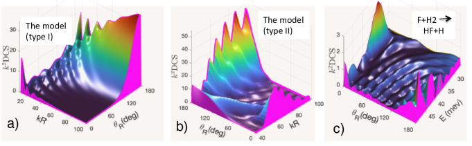
(a)

Figure 1: Dimensionless differential cross sections: a) for the model (6) with $V<0$; b) for the model (6) with $V=0$; and c) for the $F+H_{2}(0,0,0)\to HF(2,0,0)+H$ reaction [40]. (Note the different orientations of the plots, chosen to reveal the features of interest, as discussed further in the text.)

The integral cross-sections for these three systems were analysed in [56]. Below we will use the same systems as examples in our analysis of angular distributions.

2.2 Scattering ”interferometry”

The differential cross sections in Figure 1 exhibit complicated interference patterns which may be used to gain further insight into what happens in the course of a reaction. In fact, the DCS appear to be more sensitive to the details of the scattering mechanism that their total (integral) counterparts [56]. To see why, and in order to introduce useful terminology, we start by revisiting scattering of a single classical particle by a short-ranged central potential $V(r)$ (see Figure 2a)). The trajectory of the particle with a given impact parameter lies in a plane, perpendicular to its angular momentum $J$, and the scattering angle $\theta$ is the angle between the particle’s initial and final velocities $v_{I}$ and $v_{F}$. Also relevant to our analysis, is the winding angle $\varphi$ swept by the vector $\vec{R}$, drawn to the particle from the origin, before it settles into its final direction $\vec{R}^{F}$. Clearly, the two are related by $\theta=\pi-\varphi$. Consider next a trajectory with a different impact parameter (not shown in Figure 2a)), which probes an attractive part of the potential, so that $\vec{R}$ rotates by $\varphi=\theta+\pi$. With a beam of particles incident on the potential, there will be a similar trajectory passing the scatterer on the other, ”far” side, and ending in the same detector as the ”nearside” (NS) trajectory with $\varphi=\pi-\theta$ (see Figure 3). Other possibilities include NS trajectories orbiting the potential $M=0,1,2,...$ times, so that we have $\varphi=\pi-\theta+2M\pi$, and the ”farside” (FS) trajectories with $\varphi=\pi+\theta+2M\pi$. The presence, or otherwise, of such trajectories will, of course, depend on the properties of the potential, and the energy $E$ of the incident beam.

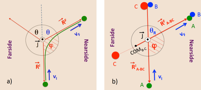
(a)

Figure 2: a) A classical particle scattered by a central potential. In the course of the collision the particle’s position vector $\vec{R}$ rotates by an angle $\varphi<\pi$, the scattering angle is $\theta=\pi-\varphi$, and the trajectory is of the $1$-st nearside type. By symmetry, a similar trajectory (not shown, see Figure 3, for which $\vec{R}$ (dashed) rotates by an angle $\varphi=\pi+\theta$, contributes to the same scattering angle, and is of the first far side type. In quantum mechanics, probability amplitudes for the two routes should be added, when calculating the probabilities.
b) The initial and final arrangements for a reactive scattering ($A+BC\to AB+C$) into an angle $\theta_{R}$. Projection of the reactants’s Jacobi vector $\vec{R}_{A-BC}$ onto the plane, perpendicular to the total angular momentum $\vec{J}$, sweeps an angle $\varphi<\pi$, and the corresponding trajectory is of the $1$-st nearside type.

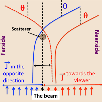
(a)

Figure 3: A beam of particle is incident on a central potential. Two trajectories (solid), passing on the opposite sides of the scatterer with different impact parameters (angular momenta) experience repulsion and attraction, respectively, and are deflected into the same scattering angle $\theta$. By symmetry, the one passing on the left of the target has a right hand side counterpart (dashed), corresponding to the same scattering angle. It is, therefore, sufficient (and convenient) to consider only the processes where a particle passes on the same side of the target, but may exit into the nearside, or the farside zone.

A classical analysis of atom-diatom reactive scattering turns out to be remarkably similar despite a larger number of variables involved [32]. For our purpose, it is sufficient to consider only the angle swept by the projection of the Jacobi vector $\vec{R}_{A-BC}$, drawn from the COM of the $BC$ pair to the atom $A$, onto the plane perpendicular to the total angular momentum $\vec{J}$ (this now includes the orbital component $\vec{\ell}$, as well as the molecule’s own angular momentum $\vec{j}$) [32]. In the zero-helicity case (3)-(4), the initial and final directions of $\vec{R}_{A-BC}$ (although not necessarily its intermediate orientations) are both perpendicular to $\vec{J}$, as shown in Figure 2b). Note that even though the atoms $B$ and $C$ are separated after the reaction, $\vec{R}_{A-BC}$ eventually settles into a final direction, opposite to the products’ Jacobi vector $\vec{R}_{C-AB}$ drawn from the COM of $AB$ to $C$. As in the case of potential scattering, three-particle reactive trajectories can be classified according to the value of the winding angle $\varphi$, acquired in the course of the reaction. In particular, one has a $M+1$-st nearside reactive trajectory, leading to a scattering angle $\theta_{R}$, if

$$\varphi^{NS}_{M}=(2M+1)\pi-\theta_{R},\quad 0<\theta_{R}<\pi,\quad M=0,1,2...,\quad\quad\quad$$ (7)

and a $M+1$-st farside reactive trajectory, leading to a scattering angle $\theta_{R}$, if

$$\varphi^{FS}_{M}=(2M+1)\pi+\theta_{R},\quad 0<\theta_{R}<\pi,\quad M=0,1,2...\quad\quad\quad$$ (8)

Classically, the detection rate of particles (or diatomic molecules) scattered into an angle $\theta$ (or $\theta_{R}$) is obtained by adding the numbers of particle travelling via all the trajectories leading to the same angle $\theta_{R}$. Quantally, one adds the amplitudes of all scenarios leading to the same outcome, and takes the absolute square of the result. The use of the interference patterns which may occur in a DCS, in order to understand the reaction’s mechanism, is the main rationale behind the development of the software described in this article.

2.3 A simple nearside-farside decomposition of the scattering amplitude

A simple method for separating the scattering amplitude (3)-(4) into the nearside and farside components originated in nuclear and heavy-ion physics [55] was first applied to molecular collisions and chemical reactions in [30], [33] and [34]. It is based on approximating Legendre polynomials in the PWS (4) by a sum of two components,

$$P_{J}(cos(\theta_{R}))\approx P_{J}^{+}(\theta_{R})+P_{J}^{-}(\theta_{R}),$$ (9)

where

$$P_{J}^{\pm}(\pi-\theta_{R})\equiv[2\pi(J+1/2)\sin(\pi-\theta_{R})]^{-1/2}$$ (10)

$$\times\exp\{\pm i[(J+1/2)(\pi-\theta_{R})-\pi/4]\}.$$

Accordingly, the scattering amplitude is written as a sum of two terms,

$$f_{\nu^{\prime}\leftarrow\nu}(\theta_{R},E)=f^{NS}_{\nu^{\prime}\leftarrow\nu}(\theta_{R},E)+f^{FS}_{\nu^{\prime}\leftarrow\nu}(\theta_{R},E),$$ (11)

where

$$f^{NS,FS}_{\nu^{\prime}\leftarrow\nu}(\theta_{R},E)=(ik_{\nu})^{-1}\sum_{J=0}^{\infty}(J+1/2)S^{J}_{\nu{{}^{\prime}}\leftarrow\nu}P^{\pm}_{J}(\pi-\theta_{R}).$$ (12)

Since Eqs. (9)-(10) are valid in an angular range

$$J\sin(\theta_{R})>>1,$$ (13)

the approximation is useful in a ”semiclassical limit”, where the PWS (11) converges after sufficiently large number of terms (in practice, $J_{max}\gtrsim 10$), and the reaction is dominated by large total angular momenta. The possibility of extending the decomposition to low values of $J$ and non-zero helicities was discussed, for example, in [34], but such an extension is beyond the scope of our analysis.) The simple NS-FS decomposition (11) inevitably fails for forward, $\theta_{R}\approx 0$, and backward, $\theta_{R}\approx\pi$ directions.
In summary, an interference pattern appearing in $f_{\nu^{\prime}\leftarrow\nu}(\theta_{R},E)$, with both $f^{NS}_{\nu^{\prime}\leftarrow\nu}(\theta_{R},E)$ and $f^{FS}_{\nu^{\prime}\leftarrow\nu}(\theta_{R},E)$ remaining smooth function of $\theta_{R}$, indicates the importance of virtual scenarios in which the Jacobi vector $\vec{R}_{A-BC}$ rotates by an angle $\varphi>\pi$.
However, the just described simple technique cannot distinguish between the scenarios in which $\vec{R}_{A-BC}$ completes several full rotations before settling into its final direction [cf. Eqs.(7) and (8)], and can be improved further.

2.4 A detailed nearside-farside decomposition of the scattering amplitude. Forward and backward scattering

A further insight into the reaction’s mechanism can be gained if the behaviour of the $S$-matrix element is known on the entire positive $J$-axis ($J\equiv|\vec{J}$). One can define a function $S_{\nu{{}^{\prime}}\leftarrow\nu}(\lambda)$,

$$\lambda\equiv J+1/2,$$ (14)

analytic in the whole complex $\lambda$-plane, such that the $S^{J}_{\nu{{}^{\prime}}\leftarrow\nu}$ in the PWS (3) are its values at non-negative half-integer $\lambda$’s, $S^{J}_{\nu{{}^{\prime}}\leftarrow\nu}=S_{\nu{{}^{\prime}}\leftarrow\nu}(J+1/2)$, $J=0,1,2...$ (We will use either $J$ or $\lambda$, whichever makes an expression look simpler). It can then be shown [40] that it is sufficient to know two functions of the winding angle $\varphi$, namely

$$\tilde{f}(\varphi)=\int_{0}^{\infty}\sqrt{\lambda}S_{\nu{{}^{\prime}}\leftarrow\nu}(\lambda)\exp(i\lambda\varphi)d\lambda$$ (15)

and

$$\tilde{g}(\varphi)=\int_{0}^{\infty}\lambda S_{\nu{{}^{\prime}}\leftarrow\nu}(\lambda)\exp(i\lambda\varphi)d\lambda,$$ (16)

in order to be able to analyse the behaviour of the scattering amplitude in the whole angular range.
In particular, with the help of the Poisson sum formula [55], the NS and FS parts of the scattering amplitude (11) can be written as [40]

$$f^{NS}_{\nu^{\prime}\leftarrow\nu}(\theta_{R},E)=\sum_{M=-\infty}^{\infty}f^{NS}_{\nu^{\prime}\leftarrow\nu}(\theta_{R},E|M)=\quad\quad\quad\quad\quad\quad\quad\quad\quad\quad\quad\quad$$ (17)

$$(ik_{\nu})^{-1}[2\pi\sin(\theta_{R})]^{-1/2}\sum_{M=-\infty}^{\infty}\tilde{f}(\varphi^{NS}_{M})\exp[-i(M+1/4)\pi],$$

$$f^{FS}_{\nu^{\prime}\leftarrow\nu}(\theta_{R},E)=\sum_{M=-\infty}^{\infty}f^{FS}_{\nu^{\prime}\leftarrow\nu}(\theta_{R},E|M)=\quad\quad\quad\quad\quad\quad\quad\quad\quad\quad\quad\quad$$

$$(ik_{\nu})^{-1}[2\pi\sin(\theta_{R})]^{-1/2}\sum_{M=-\infty}^{\infty}\tilde{f}(\varphi^{FS}_{M})\exp[-i(M+3/4)\pi],$$

where the angles $\varphi^{NS}_{M}$ and $\varphi^{FS}_{M}$ are defined in Eqs.(7) and (8), respectively, and $M$ is allowed to take negative values. It is readily seen that the individual terms in the r.h.s. of Eqs.(17) correspond to the processes in which $\vec{R}_{A-BC}$ undergoes $M$ complete rotations before settling into its final direction. The full NS or FS amplitude is, therefore, a result of interference between all such terms. Like the simple NS-FS decomposition (11), Eqs.(17) are best used in the semiclassical case $J_{max}\gtrsim 10$, and for $\theta_{R}$ not too close to either $0$ or $\pi$.
Similar decompositions of the amplitudes for small, $\theta_{R}\approx 0$, and large $\theta_{R}\approx\pi$ are obtained with the help of the second ”unfolded amplitude”, $\tilde{g}(\varphi)$, defined in Eq.(16),

$$f_{\nu^{\prime}\leftarrow\nu}(\theta_{R}\approx 0,E)=-\frac{[\theta_{R}/\sin(\theta_{R})]^{1/2}}{\pi k_{\nu}}\sum_{M=-\infty}^{\infty}(-1)^{M}\times\quad\quad\quad\quad\quad\quad$$ (18)

$$\int_{-\theta_{R}}^{\theta_{R}}\frac{\tilde{g}(\varphi+(2M+1)\pi)}{\sqrt{\theta_{R}^{2}-\varphi^{2}}}d\varphi,\quad\quad$$

$$f_{\nu^{\prime}\leftarrow\nu}(\theta_{R}\approx\pi,E)=\frac{[(\pi-\theta_{R})/\sin(\theta_{R})]^{1/2}}{i\pi k_{\nu}}\sum_{M=-\infty}^{\infty}(-1)^{M}\times\quad\quad\quad\quad\quad\quad$$

$$\int_{-(\pi-\theta_{R})}^{(\pi-\theta_{R})}\frac{\tilde{g}(\varphi+2\pi M))}{\sqrt{\theta_{R}^{2}-\varphi^{2}}}d\varphi.\quad$$

For the forward, $\theta_{R}=0$, and backward, $\theta_{R}=\pi$, scattering amplitudes Eqs. (18) yield [40]

$$f_{\nu^{\prime}\leftarrow\nu}(\theta_{R}=0,E)=\sum_{M=-\infty}^{\infty}f^{FW}_{\nu^{\prime}\leftarrow\nu}(E|M)=-k^{-1}_{\nu}\sum_{M=-\infty}^{\infty}(-1)^{M}\tilde{g}((2M+1)\pi),$$ (19)

and

$${\color[rgb]{0,0,0}f_{\nu^{\prime}\leftarrow\nu}(\theta_{R}=\pi,E)=\sum_{M=-\infty}^{\infty}f^{BW}_{\nu^{\prime}\leftarrow\nu}(E|M)=}(ik_{\nu})^{-1}\sum_{M=-\infty}^{\infty}(-1)^{M}\tilde{g}(2M\pi).$$ (20)

Now the individual terms in Eqs.(19) and (20) correspond to the scenarios in which $\vec{R}_{A-BC}$ settles in the forward or backward direction after $M$ complete rotations. Note that both clockwise and anti-clockwise rotation are, in principle, possible. The regions of applicability of Eqs. (17) and (18) overlap [35], so that one has representations of the relative scattering amplitude in the entire angular range $0\leq\theta_{R}\leq\pi$.
The full dynamical information is, however, contained in the $S$-matrix elements and, therefore, in the amplitudes $\tilde{f}(\varphi)$ and $\tilde{g}(\varphi)$, whose properties we discuss next.

2.5 Direct scattering amplitude. Primitive semiclassical approximation and the deflection function

The forces acting between the collision partners are typically repulsive and, in the absence of other processes, one may expect that $\vec{R}_{A-BC}$ would rotate by an angle $\overline{\varphi}(J)$, $\pi\leq\overline{\varphi}(J)\leq 0$, where $\overline{\varphi}(J)$ is uniquely defined by the value of $J$. The small angular momenta correspond to a nearly head-on-collisions, where the collision partners bounce back after exchanging the atom $B$. In this case, we have $\overline{\varphi}(J\approx 0)\approx 0$ and $\theta_{R}\approx\pi$. At large angular momenta, $J>>1$, collision partners pass each other at a distance, and the transfer of the atom $B$ is suppressed. In this limit, we have $\overline{\varphi}(J>>1)\approx\pi$, and $\theta_{R}\approx 0$. The $S$-matrix element can be written as $S_{\nu{{}^{\prime}}\leftarrow\nu}(\lambda)=|S_{\nu{{}^{\prime}}\leftarrow\nu}(\lambda)|\exp[i\Theta_{\nu{{}^{\prime}}\leftarrow\nu}(\lambda)]$, where the first factor, $|S_{\nu{{}^{\prime}}\leftarrow\nu}(\lambda)|_{\lambda\to\infty}\to 0$, for the reason just discussed. The rapidly changing phase $\Theta_{\nu{{}^{\prime}}\leftarrow\nu}(\lambda)$ determines the final orientation of $\vec{R}_{A-BC}$. In particular, we have [32]

$$d\Theta_{\nu{{}^{\prime}}\leftarrow\nu}(\lambda)/d\lambda=-\overline{\varphi}(\lambda).$$ (21)

If $d\Theta_{\nu{{}^{\prime}}\leftarrow\nu}(\lambda)/d\lambda$ happens to be a smooth decreasing function, relation (21) can be inverted, to define angular momentum, $\overline{\lambda}(\varphi)$, as a function of the unique winding angle $\varphi$. Evaluating the integrals (15) and (16) with the help of the stationary phase approximation, we have (for simplicity, we omit the hessians and various other factors, as these expressions are not used by our code)

$$\tilde{f}(\varphi)\sim\sqrt{\overline{\lambda}(\varphi)}|S_{\nu{{}^{\prime}}\leftarrow\nu}(\overline{\lambda}(\varphi))|\exp[i\Theta_{\nu{{}^{\prime}}\leftarrow\nu}(\overline{\lambda}(\varphi))],$$ (22)

$$\tilde{g}(\varphi)\sim{\overline{\lambda}(\varphi)}|S_{\nu{{}^{\prime}}\leftarrow\nu}(\overline{\lambda}(\varphi))|\exp[i\Theta_{\nu{{}^{\prime}}\leftarrow\nu}(\overline{\lambda}(\varphi))].\quad$$

From the previous discussion it is clear, that both functions will be contained mostly in the region $0\leq\varphi\leq\pi$, with $|\tilde{f}(\varphi)|$ and $|\tilde{g}(\varphi)|$ decreasing as $\varphi$ increases. We will call the region $0\leq\varphi\leq\pi$ the first nearside zone and note, in addition, that in this simple case the sums in Eqs.(17) are reduced to just one term,

$$f_{\nu^{\prime}\leftarrow\nu}(\theta_{R},E)\approx(ik_{\nu})^{-1}[2\pi\sin(\theta_{R})]^{-1/2}\tilde{f}(\varphi^{NS}_{0})\exp[-i\pi/4],$$ (23)

and

$$f_{\nu^{\prime}\leftarrow\nu}(\theta_{R}=0,E)\approx-k^{-1}_{\nu}\tilde{g}(\pi),\quad\quad$$ (24)

$$f_{\nu^{\prime}\leftarrow\nu}(\theta_{R}=\pi,E)=(ik^{-1}_{\nu})\tilde{g}(0)\approx 0.$$

One useful quantity is the deflection function, obtained by adding a $\pi$ to both sides of Eq.(21), which now yields the (unique) reactive scattering angle, for each value of the total angular momentum,

$$\theta_{R}(\lambda,E)=\pi-\frac{d\Theta_{\nu{{}^{\prime}}\leftarrow\nu}(\lambda)}{d\lambda}.$$ (25)

A typical deflection function would, therefore, start from $\pi$ at $\lambda\approx 1/2$, and then decrease to zero, often almost linearly, in the whole range of the angular momenta which contribute to the reaction [38].
The simple situation just described does not always occur in practice. For example, in Figure 1 direct scattering occurs only at higher energies ($kR\gtrsim 50$) in the panel a). Deflection function exhibiting a minimum, or crossing to negative value would indicate the presence of rainbow [42]-[44], or glory [45]-[47] effects in the DCS. There is, however, an alternative universal language, relating such effects to the singularities of the $S$-matrix element. We will consider them next.

2.6 Resonances and Regge poles

In our analysis, an important role is played by the (Regge) poles of the $S$-matrix, $S_{\nu^{\prime}\leftarrow\nu}(E,J)$ in the first quadrant of the complex $J(\lambda)$-plane. A process in which the products form a long-lived triatomic ”quasi-molecule”, which breaks up into products after several complete rotations, manifests itself as a pole close to the real $J$-axis, in the first quadrant of the complex $J$-plane,

$$S_{\nu^{\prime}\leftarrow\nu}(E,J_{n})=\infty,\quad ReJ_{n}>0,\quad ImJ_{n}>0.$$ (26)

The real part of the pole’s position is related to the angular velocity, at which the quad-molecule spins. Its imaginary part, $ImJ_{n}$, defines the complex’s angular life - a typical angle by which it rotates before breaking up.
The complex must rotate in order to preserve the total angular momentum, which causes the Jacobi vector $\vec{R}_{A-BC}$ to sweep a winding angle $\varphi>\pi$ as the complex decays into the first farside, the second nearside, the second farside, and so on, zones. Typically (at least for $J_{max}>>j,j^{\prime}$) the intermediate triatomic needs to rotate in the positive sense around $\vec{J}$ (counter-clockwise, if $\vec{J}$ is pointing towards the observer), which explains why the Regge poles are confined to the first quadrant of the complex $J$-plane. Indeed, it is easy to show [40] that, in presence of several ($N_{res}$) resonance Regge poles at $J_{n}$ ($\lambda_{n}=J_{n}+1/2$), the two functions in Eqs. (15) and (16), have a particularly simple form beyond the first nearside zone, i.e., for $\varphi>\pi$,

$$\tilde{f}(\varphi)\approx\sum_{n=1}^{N_{res}}\tilde{f}^{(tail)}_{n}(\varphi)=2\pi i\sum_{n=1}^{N_{res}}\sqrt{\lambda_{n}}Res[S_{\nu^{\prime}\leftarrow\nu}(E,\lambda_{n})]\exp(i\lambda_{n}\varphi),$$ (27)

$$\tilde{g}(\varphi)\approx\sum_{n=1}^{N_{res}}\tilde{g}^{(tail)}_{n}(\varphi)=2\pi i\sum_{n=1}^{N_{res}}{\lambda_{n}}Res[S_{\nu^{\prime}\leftarrow\nu}(E,\lambda_{n})]\exp(i\lambda_{n}\varphi),\quad$$

where $Res[S_{\nu^{\prime}\leftarrow\nu}(E,\lambda_{n})]$ is the residue of the $S$-matrix element at the $n$-th Regge pole,

$$S_{\nu^{\prime}\leftarrow\nu}(E,\lambda_{n})\to\frac{Res[S_{\nu^{\prime}\leftarrow\nu}(E,\lambda_{n})]}{\lambda-\lambda_{n}},\quad\lambda\to\lambda_{n}=J_{n}+1/2.$$ (28)

Thus, outside the first nearside zone, a pole creates an ”exponential tail” $\sim\exp\{i\text{Re}[\lambda_{n}]\varphi-\text{Im}[\lambda_{n}]\varphi\}$, describing the rotation of a triatomic complex, accompanied by an exponential decay. Note that a similar pole in the fourth quadrant of the complex $J$-plane, $\text{Im}[\lambda_{n}]>0$, $\text{Im}[\lambda_{n}]<0$, would describe an unphysical increase, rather than a decay, and for this reason the physical poles have to lie above the real $J$-axis. In our semiclassical treatment, a capture into a long-lived intermediate state occurs at a total angle momentum $J\sim\text{Re}[J_{n}]$, corresponding to a direct scattering $\varphi_{n}$. In the vicinity of this winding angle direct scattering cannot be distinguished from the immediate decay of the newly formed complex [31]. At larger $\varphi$’s, still in the first NS zone, it may be possible to tell these contributions apart in both $\tilde{f}(\varphi)$ and $\tilde{g}(\varphi)$. Although a reasonably simple description of the behaviour of the two functions in the first NS zone can thus be obtained [40], including it in a computer program is not straightforward, and we will concentrate instead on the $\varphi\geq\pi$ angular range, where the direct component is usually absent [cf. Eqs.(25)]. Bearing in mind that the Jacobi vector $\vec{R}_{A-BC}$ rotates predominantly in the positive direction around the total angular momentum $\vec{J}$, we can start the summation in Eqs.(17), (19) and (20) from $M=0$. With the help of Eq.(27) the sideway (SW) scattering amplitude can be written as

$$f_{\nu^{\prime}\leftarrow\nu}(0<\theta_{R}<\pi,E)\approx f^{NS}_{\nu{{}^{\prime}}\leftarrow\nu}(\theta_{R},E|0)+2\pi k_{\nu}^{-1}[2\pi\sin(\theta_{R})]^{-1/2}\times$$ (29)

$$\sum_{n=1}^{N_{res}}\sum_{K=0}^{\infty}\sqrt{\lambda_{n}}Res[S_{\nu^{\prime}\leftarrow\nu}(E,\lambda_{n})]\ \exp[i(\lambda_{n}\varphi_{K}-K\pi/2-\pi/4)]$$

$$\equiv f^{NS}_{\nu{{}^{\prime}}\leftarrow\nu}(\theta_{R},E|0)+\sum_{n=1}^{N_{res}}\sum_{K=0}^{\infty}f^{SW(tail)}_{\nu^{\prime}\leftarrow\nu,n}(\theta_{R},E|K)\quad\quad$$

$$\equiv f^{NS}_{\nu{{}^{\prime}}\leftarrow\nu}(\theta_{R},E|0)+\sum_{n=1}^{N_{res}}f^{SW(tail)}_{\nu^{\prime}\leftarrow\nu,n}(\theta_{R},E),\quad\quad\quad\quad$$

where $\varphi_{K}=(-1)^{K+1}\theta_{R}+\pi\{K+[(-1)K+1]/2\}$, $K=1,2...$. (Note that for an odd $K$, $\varphi$ lies in the $K$-th FS zone, whereas $f^{SW}_{\nu^{\prime}\leftarrow\nu,n}(\theta_{R},E|K)$ is what the $n$-th pole contributes in the $K$-th farside zone (see Figure 4). Now the first term in Eq.(29) corresponds to a process in which $\vec{R}_{A-BC}$ rotates by a $\varphi<\pi$, while the second term includes the contributions from $N_{res}$ rotating complexes beyond the first NS zone, i.e., for $\varphi>\pi$.

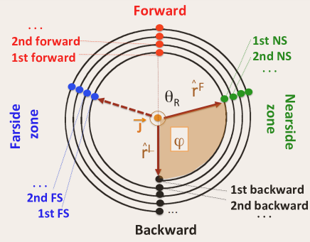
(a)

Figure 4: Possible rotations of a vector $\hat{r}\equiv\vec{R}_{A-BC}/|\vec{R}_{A-BC}|$ around the total angular momentum $\vec{J}$, directed towards the viewer. In the semiclassical limit, the vector is expected to rotate in the positive sense, i.e., counter-clockwise.

By the same token, the forward (FW) and the backward (BW) scattering amplitudes, (19) and (20), can be approximated by

$$f_{\nu^{\prime}\leftarrow\nu}(\theta_{R}=0,E)=-k^{-1}_{\nu}\sum_{n=1}^{N_{res}}\sum_{M=0}^{\infty}(-1)^{M}\tilde{g}^{(tail)}_{n}((2M+1)\pi)$$ (30)

$$\equiv\sum_{n=1}^{N_{res}}\sum_{M=0}^{\infty}f^{FW(tail)}_{\nu^{\prime}\leftarrow\nu,n,M}(E)\equiv\sum_{n=1}^{N_{res}}f^{FW(tail)}_{\nu^{\prime}\leftarrow\nu,n}(E)\quad\quad$$

and

$$f_{\nu^{\prime}\leftarrow\nu}(\theta_{R}=\pi,E)=(ik_{\nu})^{-1}\left[\tilde{g}(0)+\sum_{n=1}^{N_{res}}\sum_{M=1}^{\infty}(-1)^{M}\tilde{g}^{(tail)}_{n}(2M\pi)\right]\quad\quad$$ (31)

$$\equiv f^{BW(direct)}_{\nu^{\prime}\leftarrow\nu}+\sum_{n=1}^{N_{res}}\sum_{M=1}^{\infty}f^{BW(tail)}_{\nu^{\prime}\leftarrow\nu,n,M}(E)\equiv f^{BW(direct)}_{\nu^{\prime}\leftarrow\nu}+\sum_{n=1}^{N_{res}}f^{BW(tail)}_{\nu^{\prime}\leftarrow\nu,n}(E).$$

In Eq.(31), $\tilde{g}(0)$ describes a direct recoil in a head-on collision, while $\tilde{g}((2M+1)\pi)$, $M\geq 0$, and $\tilde{g}(2M\pi)$, $M\geq 1$, correspond to the processes in which a rotating complex decays into the $\theta_{R}=0$ and $\theta_{R}=\pi$ directions after several complete rotations. A typical situation is shown in Figure 5, and Figure 6 shows how the unfolded amplitudes $\tilde{f}(\varphi)$ and $\tilde{g}(\varphi)$ can be ”folded back” to produce a scattering amplitude $f_{\nu^{\prime}\leftarrow\nu}(\theta_{R},E)$ at a given angle $\theta_{R}$.

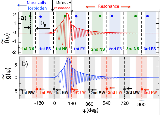
(a)

Figure 5: The ”unfolded” scattering amplitudes: a) the $\tilde{f}(\varphi)$ and b) $\tilde{g}(\varphi)$, for the $F+HD(0,0,0)\to HF(3,0,0)+D$ reaction at $E=97.5$ $mev$ [57]. The PWS sum (3) converges for $N_{max}\gtrsim 30$, and the semiclassical treatment applies. Also indicated are (a) various near- and farside zones, as well as (b) the winding angles contributing to the forward, ($\theta_{R}=0$) and backward, ($\theta_{R}=\pi$), scattering amplitudes.

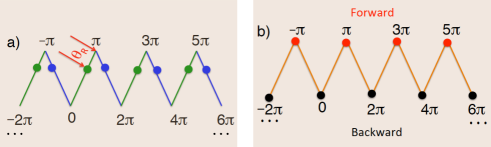
(a)

Figure 6: Folding back the unfolded amplitudes in Figure 4. a) The values of $\tilde{f}(\varphi)$ for the $\varphi$’s corresponding to the same $\theta_{R}$ are added [with appropriate phase factors, cf. Eqs.(17)] to produce a sideway amplitude $f_{\nu{{}^{\prime}}\leftarrow\nu}(\theta_{R})$, $0<\theta_{R}<\pi$. b) The values of $\tilde{g}(\varphi)$ for the $\varphi$’s corresponding to the same $\theta_{R}=0$ ($\theta_{R}=\pi$) are added [with appropriate signs, cf. Eqs.(19)-(20)] to produce a forward (backward) scattering amplitude $f_{\nu{{}^{\prime}}\leftarrow\nu}(\theta_{R}=0)$ ( $f_{\nu{{}^{\prime}}\leftarrow\nu}(\theta_{R}=\pi)$).

Geometric progressions in Eqs.(30) and (31) can be summed explicitly, to yield

$$f^{FW(tail)}_{\nu^{\prime}\leftarrow\nu,n}(E)=-\frac{2\pi i}{k_{\nu}}{\lambda_{n}}Res[S_{\nu^{\prime}\leftarrow\nu}(E,\lambda_{n})]\frac{\exp(i\pi\lambda_{n})}{1+\exp(2\pi i\lambda_{n})}$$ (32)

and

$$f^{BW(tail)}_{\nu^{\prime}\leftarrow\nu,n}(E)=-\frac{2\pi}{k_{\nu}}{\lambda_{n}}Res[S_{\nu^{\prime}\leftarrow\nu}(E,\lambda_{n})]\frac{1}{1+\exp(-2\pi i\lambda_{n})}.$$ (33)

Thus, Eq.(32) accounts for all forward contributions in Figure 4, while Eq.(33) results from summing all but the first backward contribution in Figure 4.
Similarly, summing the two geometric progressions (for the NS and FS contributions) yields

$$f^{SW(tail)}_{\nu^{\prime}\leftarrow\nu,n}(\theta_{R},E)=\sqrt{\frac{2\pi}{k_{\nu}^{2}\sin(\theta_{R})}}{\lambda_{n}^{1/2}}Res[S_{\nu^{\prime}\leftarrow\nu}(E,\lambda_{n})]\times$$ (34)

$$\exp(-i\pi/4)\left[\frac{\exp[i\lambda_{n}(\pi-\theta_{R})]}{1+\exp(-2\pi i\lambda_{n})}-i\frac{\exp[i\lambda_{n}(\pi+\theta_{R})]}{1+\exp(2\pi i\lambda_{n})}\right].$$

Note that the amplitudes for the capture in a particular metastable state are always added, and one cannot determine which complex has been formed just as one cannot know which of the two slits was chosen by a particle in a Young’s double-slit experiment [58].
Finally, it is worth noting that in quantum mechanics, formation of a long-lived complex may involve classically forbidden processes, such as tunnelling across potential barriers. Such shape resonances, not seen in simulations employing classical trajectories, will manifest themselves as Regge poles in the first quadrant of the CAM plane. A description in terms of poles is also possible for rainbow [38] and glory [37] effects, where a sequence of poles, rather just a single pole, are responsible for the structure in the deflection function (25). Application of the methods, described above in subsections 2.4-2.6 requires the knowledge of the behaviour of the $S$-matrix element in a subset of the complex $J$-plane, which is not readily provided by the scattering codes. Thus, an analytic continuation of $S_{\nu^{\prime}\leftarrow\nu}(E,J_{n})$ is a necessary element of our analysis.

2.7 Padé reconstruction of the scattering matrix element

The application of the equations (15)-(34) requires the knowledge of the pole positions $\lambda_{n}=J_{n}+1/2$, and the corresponding residues, $Res[S(E,\lambda_{n})]$. A computer code used in modelling a chemical reaction typically evaluates the $S$-matrix elements, $S^{J}_{\nu{{}^{\prime}}\leftarrow\nu}(E)$, for the physical integer values of $J=0,1,2,...N$, with $N$ sufficiently large to converge the partial waves sum (3). Using these values, we construct a rational Padé approximant, ($[x]$ denotes integer part of $x$)

$$S_{\nu^{\prime}\leftarrow\nu}^{Pade}(E,J)\equiv K_{N}\textrm{exp}[i(aJ^{2}+bJ+c)]\times\frac{\prod_{i=1}^{[N/2]}(J-Z_{i})}{\prod_{i=1}^{[(N-1)/2]}(J-P_{i})},$$ (35)

where $P_{i}(E)$ and $Z_{i}(E)$ stand for poles and zeroes of the approximant, respectively, and $K_{N}(A)$, $a(E)$, $b(E)$ and $c(E)$ are energy dependent constants. The approximant is conditioned to coincide with $S(E,J)$ at the $N$ integer values of $J$,

$$S_{\nu^{\prime}\leftarrow\nu}^{Pade}(E,J)=S^{J}_{\nu^{\prime}\leftarrow\nu}(E),\quad J=0,1,...N,$$ (36)

and provides an analytic continuation for the exact function $S_{\nu^{\prime}\leftarrow\nu}(E,J)\approx S_{\nu^{\prime}\leftarrow\nu}^{Pade}(E,J)$ in a region of the complex $J$-plane, containing the supplied values $S^{J}_{\nu^{\prime}\leftarrow\nu}(E)$. Inside this region, the poles and zeroes of the approximant serve as good approximation to the true Regge poles and zeroes of the $S$-matrix element. The remaining poles and zeroes tend to mark the border of the region, beyond which Padé approximation fails [38],[53]. Thus, for a given pole $J_{n}=P_{j}$, the residue is given by

$$Res[S_{\nu^{\prime}\leftarrow\nu}(E,\lambda_{n})]=K_{N}\textrm{exp}[i(aP_{j}^{2}+bP_{j}+c)]\times\frac{\prod_{i=1}^{[N/2]}(P_{j}-Z_{i})}{\prod_{i=1,i\neq j}^{[(N-1)/2]}(P_{j}-P_{i})},$$ (37)

which, together with Eq.(35) provides all the data required for our analysis.
The program used to construct the Padé approximant (35) is the PADE_II code described in the Refs. [53] and [56].

2.8 A brief summary

Our analysis consists in representing a reactive scattering amplitude (3) by a sum of simpler sub-amplitudes. It is used to relate the interference patterns observed in a reactive DCS to the details of the reaction’s mechanism, such as capture of the collision partners into long- and not-so-long-lived intermediate states. The present approach can be applied in the case of zero initial and final helicities. In particular, the DCS_Regge code performs the following tasks.
A) Evaluate the simple nearside-farside decomposition (11)-(12) in a specified energy range.
B) Analytically continue the scattering matrix element into the complex $J(\lambda$)-plane, using its values, $S^{J}_{\nu^{\prime}\leftarrow\nu}(E)$, at $J=0,1,...$. [The user should ensure that the input values correspond to $S^{J}_{\nu^{\prime}\leftarrow\nu}(E)$ in Eq.(3), and not to $\tilde{S}^{J}_{\nu^{\prime}\leftarrow\nu}(E)=(-1)^{J}S^{J}_{\nu^{\prime}\leftarrow\nu}(E)$ in Eq.(4).]
C) With the help of the values of $S_{\nu^{\prime}\leftarrow\nu}^{Pade}(E,J)$ on the real $J$-axis, evaluate the deflection function (25) in a specified energy range.
D) With the help of the values of $S_{\nu^{\prime}\leftarrow\nu}^{Pade}(E,J)$ on the real $J(\lambda)$-axis, evaluate the ”unfolded amplitudes” $\tilde{f}(\varphi)$ and $\tilde{g}(\varphi)$ in Eqs. (15) and (16), in a specified energy range.
E) Use Eqs.(27) to relate the behaviour of the two amplitudes beyond the first nearside zone to the presence of Regge poles.
F) Implement the detailed nearside-farside decomposition (11), (17) of the sideways ($\theta_{R}$ is not too close to either $0$ or $\pi$) scattering amplitude in a specified energy range.  
G) Implement the decompositions (30), (31) of the forward and backward scattering amplitudes, respectively.

2.9 Limitations and some general remarks

The method aims at giving a clear picture of how the capture into metastable complexes, formed by the reactants, affects a DCS. It should, however, be noted that
$\bullet$ The DCS_Regge code is designed for analysing reactive angular distributions, and uses the reactive scattering angle $\theta_{R}$ (cf. Figure 4).
$\bullet$ The method applies to the systems for which the number of the partial waves included in the PWS is or order of $10$, or more. Note that a large number of PWs may require the use of the multiple precision option, as explained below.
$\bullet$ The analysis is limited to the zero helicity case, where the initial and final directions of $\vec{R}_{A-BC}$ both lie in the plane, perpendicular to the total angular momentum $\vec{J}$ and, classically, $\theta_{R}$ can have any value between $0$ and $\pi$. This is no longer the case if one or both helicities have non-zero values [32]. If so, $\theta_{R}$ is restricted to a narrower range, rotational matrices $d^{J}_{\Omega^{\prime}\Omega}(\pi-\theta_{R})$ develop caustics, and the semiclassical treatment becomes much more involved. Although a similar theory can, in principle, be developed, it is doubtful that its implementation be sufficiently straightforward.
$\bullet$ In its present form, the method will not also distinguish between the direct and resonance scattering into the first nearside zone, although the relevant theory can be found in [40].
$\bullet$ Our analysis is only as good as the computation used to produce the $S$-matrix elements. It cannot compensate for any shortcoming of a close-coupling calculation used in its production.
$\bullet$ However, if the $S$-matrix elements have been produced with a sufficient accuracy, so as to be in good agreement with the experimental data, our analysis would help to expose the details of the actual reaction mechanism, hidden in the PW decomposition of the scattering amplitude. For example, it would reveal a narrow resonance, falling between two integer values of the $J$, and explain the effect it has on the observed DCS.
$\bullet$ Over the years, similar methodology has been successfully applied to the $Cl+HCl$ [28, 29], $F+H_{2}/HD$ [31, 35, 39, 40] and $H+D_{2}$ [36, 37] benchmark systems. We expect the method to be well suited for a large number of various applications.
$\bullet$ The analysis cannot reveal the physical origin of the resonance (e.g., its location in the entrance or exit channel on the potential surface, etc.), which must be established independently.

3 DCS_Regge package: Overview

3.1 Installation

This version of DCS_Regge is intended for IA32 / IA64 systems running the Linux operating system. It requires Fortran and C compilers. The software is distributed in the form of a gzipped tar file, which contains the DCS_Regge source code, PADE_II 1.1 source code, QUADPACK source code, test suites for each package, as well as scripts for running and testing the code. The detailed structures of each subpackage, DCS_Regge, PADE_II 1.1 and QUADPACK, are presented in the Appendices C, D and E. For users benefits we supply a file README for each package in directories DCS, DCS/PADE and DCS/QUADPACK. The files provide a brief summary on the code structure and basic instructions for users. The DCS_Regge Manual (DCSManual.pdf), is located in the DCS/ directory whereas PADE_II Manual (FManual.pdf), can be found in the DCS/PADE directory. In addition, the documents describing PADE_II and QUADPACK are available from Mendeley Data (DOI: 10.17632/pt4ynbf5dx.1) and
http://www.netlib.org/quadpack/ respectively. Once the package is unpacked the installation should be done in the following order:

1. Installing QAUDPACK library

2. Installation of the PADE_II package

3. Installation of the DCS_Regge package.

Installation procedure for each sub-package is straightforward and can be successfully performed by following the instructions in DCS_Regge Manual. The procedure assumes using either Shell scripts (QAUDPACK) or a Makefile_UNIX file (PADE_II, DCS_Regge) with the adjusted environmental variables.

3.2 Testing

Three test suits are prepared for each sub-package to validate the installation procedure.

3.2.1 Running the QUADPACK test

To test the QUADPACK library, one has to run quadpack_prb.sh script in the /QUADPACK/scripts directory.

The results of 15 tests can be found in quadpack_prb_output.txt file in the DCS/QUADPACK/test directory. The message
QUADPACK_PRB: Normal end of execution.
confirms that the code passed the validation test.

3.2.2 Running the PADE_II test suite

The input for 4 jobs, test1, test2, test3 and test4, are provided in directories
DCS/PADE/test/input/test_name, where test_name is either test1 or test2 or test3 or test4. To submit and run a test suite, one should go to the directory DCS/PADE/test and run a script ./run_TEST. All tests will be run in separate directories. Each test takes about 1 - 5 minutes to run on a reasonably modern computer. The message
Test test_name was successful
appearing on the screen at the conclusion of the testing process confirms that the code passed the validation test test_name . The results of the simulation can be viewed in the DCS/PADE/test/output/test_name directory. The message
Your output differs from the baseline!
means that the calculated data significantly differ from that in the baselines. The files PADE/test/output/test_name/diff_file can be checked to judge the differences.

3.2.3 Running the DCS_Regge test suite

For simplicity, the test suite for DCS_Regge is designed in the similar manner as the test suite for PADE_II. The input for 3 jobs, test1, test2 and test3 are provided in directories DCS/test/input/test_name respectively, where test_name is either test1 or test2 or test3. The test suit can be run in the directory DCS/test using the following commands: ./run_TEST. All tests are run in separate directories, DCS/test/output/test1, DCS/test/output/test2 and DCS/test/output/test3. Each test takes about 1 minute to run on a reasonably modern computer. To analyse the test results, the message on the screen at the completion of the testing process has to be inspected. The message Test test_name was successful confirms that the code passed the validation test test_name. The results of the simulation can be viewed in the DCS/test/output/test_name directory. The message

test_name output differs from the baseline!

Check your output in output/test_name/basel

Baseline file: baselines/test_name/basel

Differences: output/test_name/error_file

means that the calculated data significantly differ from that in the baselines. The differences can be found in the files DCS/test/output/test_name/error_file.

4 Computational modules of DCS_Regge

4.1 Padé reconstruction and PADE_II options

As discussed above, an important part of the calculation consists in performing an analytical continuation of the $S$-matrix element into the CAM plane. The user has some flexibility in doing so. It concerns mostly the quadratic phase in Eq. (35), which must itself be determined in the course of the Padé reconstruction. The need for separating this rapidly oscillating term arises from the fact that the Padé technique used here, works best for slowly varying functions. Thus, by removing the oscillatory component, one expands the region of validity of the approximant in the CAM plane, which allows for the correct description of a larger number of poles. The extraction of the quadratic phase proceeds iteratively. Since sharp structures in the phase of the $S$-matrix element usually come from the Regge poles and zeroes located close to the real axis, one defines a strip $\texttt{-dxl}<ImJ<\texttt{dxl}$ around the real $J$-axis, and removes from the previously constructed approximant all poles and zeroes inside the strip. The smoother phase of the remainder is fitted to a quadratic polynomial, and this quadratic phase is then subtracted from the phase of the input values of $S$, after which a new approximant is constructed with these modified input data. The process is repeated niter times resulting in a (hopefully) improved Padé approximant. There is no rigorous estimate of the improvement achieved, and the practice shows that in many cases using niter > 1 gives tangible benefits, while in some cases better results are achieved with niter=$1$ or $2$. It is for the user to decide on the best values of dxl and niter for a particular problem.
The input files required for running the Padé_II code are stored in the input directory where they are labelled $1,2...N_{E}$. A typical input file is given in Figure 12 (Appendix B). The file differs from the similar input used in Padé_II package reported in [53] by one line added at the end, which should contain the collision energy in $meV$, and is identical to an input file used by ICS_Regge [56].
Other parameters for Padé reconstruction are read from the input/INPUT file.
The entry (#16) determines whether there should be a change of parity from the original data. This depends on the convention used in calculating the $S$-matrix elements, as explained in [53] (we use $0$ for no and $1$ for yes). The recommended value is $1$.
Entry (#17) decides whether one should remove the guessed values of the quadratic phase prior to the construction of the first Padé approximant in a series of iterations. Its recommended value is $1$ (yes).
Entry (#18) determines if multiple precision routines should be used in calculating the Padé approximant. The recommended value is $1$ if the number of partial waves (PW) exceeds $40$. It can also be used for a smaller number of (PW) to check the stability of calculations.
Entries (#19 and #21) allow us to repeat the calculations with added non-analytical noise of magnitude fac, nstime times. This may be needed to check the sensibility of calculations to numerical noise. The recommended initial values are nstime=0 and fac=0.00000001, in which case no noise is added.
Entry (#20) determines the number of points in the graphical output from Padé_II [53].
Finally, the user has the options of changing the number of partial waves, the number of iterations and the value of dxl for all files used in the current run by setting to $1$ iover1, iover2 and iover3 in entries (#22, #23 and #24). The corresponding parameters are reset to the values nread1, niter1, and dxl1, specified in the entries (#25, #26 and #27), respectively.

4.1.1 Changes made to PADE_II

The changes from the previous version [53] include
(I) replacement of all the Numerical Algorithms Group (NAG) routines with ones available in the public domain, and
(II) provision of additional controls allowing to change the parameters of Padé reconstruction for all energies in the run at once, without changing individual input files labelled $1$,$2$,…, as discussed in the previous Section.
A brief summary of the changes made to subroutines is given below.
Subroutine FIT (fit.f)
The NAG routine g05ccf has been replaced by a subroutine svdfit described in section 15x.4 of Numerical Recipes in C: The Art of Scientific Computing (Second Edition), published by Cambridge.

Subroutine ZSRND (zsrnd.f)
The NAG routine E02ACF has been replaced by a sequence of calls to the system routines srand48 and drand48.

Subroutine IGET_SEED (iget_seed.c)
Added new routine generating the seed for srand48.

Wrapper (wrapper.c)
Added wrapper allowing for calling C-routines IGET_SEED, srand48 and drand48 in a Fortran code.

Subroutine FINDPOLES_NAG (findpoles_NAG.f)
Removed.

Subroutine FINDZEROS_NAG (findzeros_NAG.f)
Removed.

4.2 The structure of DCS_Regge

The DCS_Regge application is a sequence of 24 FORTRAN files. The files are listed below, and their functions are explained.

Program DCS_Regge (DCS_Regge.f)
Main program.

Subroutine OPEN_IO (open_io.f)
Opens the files.

Subroutine CLOSE_IO (close_io.f)
Closes the files.

Subroutine READ1 (read1.f)
Reads the original input file at a given energy and the file screen.pade.

Subroutine READ (read.f)
Reads the parameters of the Padé reconstruction at a given energy.

Subroutine SORT (sort.f)
At a given energy, selects poles and zeroes in the specified region of the complex angular momentum ($J$-) plane and discards pole/zero pairs (Froissart doublets).

Subroutine DCS_exnearfar (dcs_exnearfar.f)
Calculates the exact DCS (3) and its simple nearside-farside decomposition (11), for a specified range of energies.

Subroutine PHASE (phase.f)
Calculates the deflection function, and the phase $\Theta_{\nu{{}^{\prime}}\leftarrow\nu}(J,E)$ of the $S$-matrix element $S_{\nu{{}^{\prime}}\leftarrow\nu}(\lambda,E)=|S_{\nu{{}^{\prime}}\leftarrow\nu}(\lambda,E)|\exp[i\Theta_{\nu{{}^{\prime}}\leftarrow\nu}(J,E)]$, for a specified range of energies.

Subroutine DCS_fg (dcs_fg)
Evaluates the unfolded amplitudes $\tilde{f}(\varphi)$ and $\tilde{g}(\varphi)$ for specified ranges of the winding angle $\varphi$ and energy E.

Subroutine DCS_side (dcs_side.f)
Evaluates the detailed near- and farside amplitudes $f^{NS}_{\nu^{\prime}\leftarrow\nu}(\theta_{R},E|M)$ and $f^{FS}_{\nu^{\prime}\leftarrow\nu}(\theta_{R},E|M)$ in Eqs.(17), for a given reactive scattering angle $\theta_{R}$, and specified ranges of $M$ and energy $E$.

Subroutine DCS_forb (dcs_forb.f)
Evaluates the decompositions of the forward and backward scattering amplitudes into $f_{\nu^{\prime}\leftarrow\nu}(\theta_{R}=0,E|M)$ and $f_{\nu^{\prime}\leftarrow\nu}(\theta_{R}=\pi,E|M)$ [cf. Eqs.(19) and (20)] for specified ranges of $M$ and energy $E$.

Subroutine REGGE1 (regge1.f)
Evaluates, for a single (first) energy $E$, the exponential tails in Eq.(27), $\tilde{f}^{tail}(\varphi|n)$ and $\tilde{g}^{tail}(\varphi|n)$, produced by a particular Regge pole at $\lambda=\lambda_{n}$ (chosen by the user) in an angular range beyond the 1-st NS zone, $\varphi\geq\pi$.

Subroutine REGGE2 (regge2.f)
For a specified range of energies E, follows the Regge trajectory, to which the pole at $\lambda=\lambda_{n}$, previously chosen by the user during the execution of REGGE1, belongs. Full contributions of the pole to the forward, backward, and sideway scattering amplitudes, (32), (33), and (34), are evaluated at each $E$, as well as the individual terms of the geometric progressions.

Function ZPADE (zpade.f)
Calculates the full Padé approximant.

Function ZPADE1 (zpade1.f)
Calculates the full Padé approximant in a different manner.

Function ZPR (zpr.f)
Evaluates the ratio of the two polynomials in the Padé approximant.

Function ZRES (zres.f)
Calculates (part of) the residue for a chosen Regge pole from the Padé approximant.

Function ZEX (zex.f)
Evaluates the partial wave sum (3).

Function ZNE (zne.f)
Evaluates the nearside partial wave sum, $f^{NS}_{\nu{{}^{\prime}}\leftarrow\nu}(\theta_{R},E)$ in Eq.(12).

Function ZFA (zfa.f)
Evaluates the farside partial wave sum, $f^{FS}_{\nu{{}^{\prime}}\leftarrow\nu}(\theta_{R},E)$ in Eq.(12).

Subroutine LPFN (lpfn.f)
Evaluates Legendre polynomials $P_{J}(\pi-\theta_{R})$ in Eq.(3).

Subroutine FNFN (fnfn.f)
Evaluates $P_{J}^{\pm}(\pi-\theta_{R})$ in Eq.(10).

Subroutine FOURIER (fourier.f)
Evaluates the Fourier transforms (15) and (16).

Function FST3 (fst3.f)
Supplies the integrand for the integral evaluated in FOURIER.

There are two additional utilities.

Subroutine SKIP (skip.f)
Decides which of the input data/energies must be included in the current run.

Subroutine SUBTR (subtr.f)
Subtracts from a forward, sideway, or backward scattering amplitude the resonance contribution from the Regge pole trajectory used by REGGE2.

All files are located in the DCS/src directory.

4.3 The QUADPACK library

QUADPACK is a FORTRAN subroutine package for the numerical computation of definite one-dimensional integrals. It originated from a joint project of R. Piessens and E. de Doncker (Appl. Math. and Progr. Div.- K.U.Leuven, Belgium), C. Ueberhuber (Inst. Fuer Math.- Techn.U.Wien, Austria), and D. Kahaner (Nation. Bur. of Standards- Washington D.C., U.S.A.) [52].
(http://www.netlib.org/quadpack/).

Currently one library subroutine, DQAGS, is used in the DCS_Regge. The subroutine estimates integrals over finite intervals using an integrator based on globally adaptive interval subdivision in connection with extrapolation [59] by the Epsilon algorithm [60]. The subroutine is called from the DCS_Regge subroutine FOURIER. For users convenience the whole library is available in the package DCS_Regge. The link to the library is provided in Makefile_UNIX in DCS/src.

5 Running the DCS_Regge code

5.1 Creating input data

Two types of input files are required for running calculations: a parameter file, INPUT, located in the DCS/input directory, and a file or a set of files for running PADE_II. The latter has(ve) to be supplied in DCS/input/PADE_data directory and it (or they) contain(s) the data to be Padé approximated. The name of directory PADE_data can be chosen arbitrary and should be specified in the parameter file INPUT before starting the calculations. The names of the input files in the directory PADE_data are fixed to be $1,2,..N_{E}$. Each file contains the input parameters required to run PADE_II, previously computed values of $S_{\nu^{\prime}\leftarrow\nu}(E,J)$ for $J=0,1,2,...J^{max}_{i}$, for the energy $E_{k}$, $k=1,2,..N_{E}$, and the value of the energy itself. An example of such an input file is given in Appendix B and also provided in the directory DCS/input.
The file DCS/input/INPUT is self-explanatory and describes each input parameter to be specified. Please notice, that each input entry appears between colons (:). For an example of the parameter file INPUT see Appendix A.

We provide input files for all test cases considered in this study under the names
DCS/input/INPUT.BOUND.DCS,
DCS/input/INPUT.BOUND.DCS.30,
DCS/input/INPUT.META.DCS,
DCS/input/INPUT.META.DCS.60,
DCS/input/INPUT.FH2, and DCS/input/INPUT.FH2.DCS.32.27.

5.2 Executing DCS_Regge

The script runDCS in the DCS/ directory automates calculations. The following assumptions are made in the script:
* all binaries for DCS_Regge are placed in DCS/bin, whereas the binaries for the PADE_II package are located in DCS/PADE/bin.
* input files are located in the directory DCS/input. The names of the input files are chosen as described in section 5.1.
* output files can be found in DCS/output on completion of a calculation.

We recommend running a calculation in the directory DCS/. The command ./runDCS immediately starts a calculation.

5.3 Understanding the run script runDCS

The run script runDCS located in the DCS/ directory does not require any tuning, editing or corrections in order to start a calculation. Provided that the parameter file DCS/input/INPUT is prepared for calculations, the run script runDCS takes care of the following steps in the following order:
1. INITIALIZATION
* Edits input parameter file INPUT
* Reads input parameters from INPUT
* Prepares directories for runs, i.e. sets useful directories and cleans existing directories if necessary.
2. BUILDING PACKAGES
* PADE_II
* DCS_Regge
* Utilities.
3. RUNNING DCS_Regge FOR ALL INPUT FILES OF INTEREST
* Checks if the input file falls in the range of energies under investigation
* Runs PADE_II with the current input file if it is in the considered range
* Runs DCS_Regge if the current input file is in the considered range
* Calculates various resonance contributions and subtracts them from the exact scattering amplitudes in order to evaluate the non-resonance (direct) background.
4. OUTPUT DATA MANAGEMENT
* Stores the calculated data in the appropriate files.

5.4 Using the code

Using the code involves at least two steps.

5.4.1 Step I

In the parameter file input/INPUT (see Appendix A) one sets
is this the first run? :yes:. The code evaluates the poles $P_{i}$ and the zeroes $Z_{i}$ of the Padé approximant (35) for each collisional energy $E_{k}$, for the chosen set of files (see #6-#7 of Appendix A), in a region of the CAM plane, $\texttt{x\_min}\leq ReP_{i},Z_{i}\leq\texttt{x\_max}$, $\texttt{y\_min}\leq ImP_{i},Z_{i}\leq\texttt{y\_max}$, with the values x_min, x_max, y_min, and y_max specified by the user in the file input/INPUT (see #12 -#15 in the Appendix A).
One has the option of not including in the Padé approximant (35) the Froissart doublets, i.e., pole-zero pairs, with the distance $|P_{i}-Z_{j}|<\texttt{$\epsilon$}$, with the value of $\epsilon$ set in #11 of Appendix A. Such pairs often represent non-analytical noise existent in the input data [61], and their removal may be beneficial.
Also, at this stage the program evaluates, for all energies, the exact DCS using Eq.(1) or (3). Provided the energy is entered in $meV$, and the reduced mass is in the $unified$ $atomic$ $mass$ $units$, ($u.a.u$ or $Daltons$) (see #10 of Appendix A), the cross sections are in the units of angstroms squared (Ų).
One then identifies Regge trajectories by plotting the pole positions vs. energy from the output file output/dcs.pole. (It is recommended to use the plot $ReP(E)$ vs. $E$, as the real parts of the pole positions are less sensitive to numerical noise). In the plot the trajectories appear as continuous strings of poles, with additional poles scattered around them in a random manner. During the first run the program:

1) Writes the exact DCS (1) vs. $\theta_{R}$ and $E$ into output/dcs.dcs3d, if dcr3D=1, and, into output/dcs.xdcs, the exact DCS vs. $\theta_{R}$ for the last energy of the range.

2) Writes $|f^{NS}_{\nu^{\prime}\leftarrow\nu}(\theta_{R},E)|^{2}$, $|f^{FS}_{\nu^{\prime}\leftarrow\nu}(\theta_{R},E)|^{2}$ and $|f^{NS}_{\nu^{\prime}\leftarrow\nu}(\theta_{R},E)+f^{FS}_{\nu^{\prime}\leftarrow\nu}(\theta_{R},E)|^{2}$ [cf. Eqs.(11) -(12) into the file output/dcs.nfdcs, for the last energy in the range.

3) Writes $|S^{Pade}_{\nu{{}^{\prime}}\leftarrow\nu}(E,J)|^{2}$ vs. $E$ and $J$ into output/dcs.prob3d if prob3D=1 (cf. Eq.(35).

4) Writes $|S^{Pade}_{\nu{{}^{\prime}}\leftarrow\nu}(E,J)|$ and $\text{Re}[S^{Pade}_{\nu{{}^{\prime}}\leftarrow\nu}(E,J)]$ vs. $J$ into output/smprod for the last energy in the range. For comparison, the input values of $|S^{J}_{\nu{{}^{\prime}}\leftarrow\nu}|$ and $\text{Re}[S^{J}_{\nu{{}^{\prime}}\leftarrow\nu}]$ [cf. Eq.(3)] vs. integer $J$ are written into output/inputvals.

5) Writes the deflection function (25) vs. $J$ and $E$ into output/dcs.ph3d, if phs3D=1.

6) Writes the deflection function (25) and the phase $\Theta_{\nu{{}^{\prime}}\leftarrow\nu}(\lambda)$ in Eq.(21) vs. $J$ into the file output/phase, for the last energy in the range.

7) Writes the first unfolded amplitude (15), $|\tilde{f}(\varphi)|$ vs. $\varphi$, $\textsf{nleft}\times\pi\leq\varphi\leq\textsf{nright}\times\pi$, and $E$ into output/dcs.f3d, if irun1=1 and dcr13D=1. (See #28-#29 of Appendix A for the values of nleft and nright.)

8) Writes the first unfolded amplitude (15), $|\tilde{f}(\varphi)|$ and $\text{Re}[\tilde{f}(\varphi)]$, vs. $\varphi$, $\textsf{nleft}\times\pi\leq\varphi\leq\textsf{nright}\times\pi$, into the file output/funf for the last energy in the range, if irun1=1. (If irun1=0, $\tilde{f}(\varphi)$ is not evaluated.)

9) Writes the second unfolded amplitude (16), $|\tilde{g}(\varphi)|$, vs. $\varphi$, $\textsf{nleft}\times\pi\leq\varphi\leq\textsf{nright}\times\pi$, and $E$ into output/dcs.g3d, if irun1=1 and dcr13D=1.

10) Writes the second unfolded amplitude (16), $|\tilde{g}(\varphi)|$ and $\text{Re}[\tilde{g}(\varphi)]$ vs. $\varphi$, $\textsf{nleft}\times\pi\leq\varphi\leq\textsf{nright}\times\pi$, into the file output/gunf for the last energy in the range, if irun1=1. (If irun1=0, $\tilde{g}(\varphi)$ is not evaluated.)

11) Writes the NS amplitudes, $|f^{NS}_{\nu{{}^{\prime}}\leftarrow\nu}(\theta_{R},E|M)|^{\textsf{npow}}$ ($\textsf{npow}=1$ or $2$) in Eqs.(17), for a chosen $\theta_{R}$ and the specified ranges of $M$ and $E$, into output/dcs.nsind.

12) Writes the FS amplitudes, $|f^{FS}_{\nu{{}^{\prime}}\leftarrow\nu}(\theta_{R},E|M)|^{\textsf{npow}}$ ($\textsf{npow}=1$ or $2$) in Eqs.(17), for a specified $\theta_{R}$ and the specified ranges of $M$ and $E$, into output/dcs.fsind.

13) For the specified range of energies, writes the exact sideway scattering amplitude, $|f_{\nu{{}^{\prime}}\leftarrow\nu}(\theta_{R},E)|^{\textsf{npow}}$ ($\textsf{npow}=1$ or $2$) in Eq.(1) and, for the specified range of $M$, $|\sum_{M}(f^{NS}_{\nu{{}^{\prime}}\leftarrow\nu}(\theta_{R},E|M)+f^{FS}_{\nu{{}^{\prime}}\leftarrow\nu}(\theta_{R},E|M)|^{\textsf{npow}}$ into output/dcs.sw.

14) Writes the forward scattering amplitudes in Eq.(19), $|f^{FW}_{\nu{{}^{\prime}}\leftarrow\nu}(E|M)|^{\textsf{npow}}$ ($\textsf{npow}=1$ or $2$), for the specified ranges of $M$ and $E$, into output/dcs.fwind.

15) For the specified range of energies, writes the exact forward scattering amplitude, $|f_{\nu{{}^{\prime}}\leftarrow\nu}(\theta_{R}=0,E)|^{\textsf{npow}}$ and, for the specified range of $M$, $|\sum_{M}f^{FW}_{\nu{{}^{\prime}}\leftarrow\nu}(E|M)|^{\textsf{npow}}$ into output/dcs.fw ($\textsf{npow}=1$ or $2$).

16) Writes the backward scattering amplitudes in Eq.(20), $|f^{BW}_{\nu{{}^{\prime}}\leftarrow\nu}(E|M)|^{\textsf{npow}}$ ($\textsf{npow}=1$ or $2$), for the specified ranges of $M$ and $E$ into output/dcs.bwind.

17) For the specified range of energies, writes the exact backward scattering amplitude, $|f_{\nu{{}^{\prime}}\leftarrow\nu}(\theta_{R}=\pi,E)|^{\textsf{npow}}$ ($\textsf{npow}=1$ or $2$) and, for the specified range of $M$, $|\sum_{M}f^{BW}_{\nu{{}^{\prime}}\leftarrow\nu}(E|M)|^{\textsf{npow}}$ into output/dcs.bw.

18) Writes into output/dcs.pole the real and imaginary parts of the poles of the Padé approximant (35) vs. $E$, within the limits specified by the user in #6-#7 of the file input/INPUT (see Appendix A). The Froissart doublets can be excluded by choosing a non-zero value of the threshold #11 of the file input/INPUT.

19) Writes into output/dcs.zero the real and imaginary parts of the zeroes of the Padé approximant (35) vs. $E$, within the limits specifies by the user in #6-#7 of the file input/INPUT (see Appendix A).

5.4.2 Step II

In the file input/INPUT one sets is this the first run? :no:. The code takes the first of the files in the energy range E_min $\leq E\leq$ E_max with E_min and E_max specified by the user in #8-#9 of the file input/INPUT (see Appendix A). It then displays all the poles at this energy within the specified range, from which the user chooses the one lying on the Regge trajectory of interest.
Next, if one sets follow trajectory by hand? :no: the code will follow the trajectory automatically, choosing at the next energy the pole whose real part is closest to that of the pole chosen at the previous energy.
If one chooses follow trajectory by hand? :yes: the program continues displaying the poles, from which the user must choose the desired one for all values of energy by hand. (The ”by hand” option is useful, e.g., when working with a poorly defined trajectory from which some of the poles may be missing.)
In both cases, the program:

1) Writes the real and imaginary parts of the chosen pole’s position [$n=1$, cf. Eq.(26)] vs. $E$ into the file output/dcs.traj.

2) Writes the real and imaginary parts of the residue (37) of the chosen pole vs. $E$ into the file output/dcs.resid.

3) For a specified $0<\theta_{R}<\pi$ writes into the file output/dcs.swtind $|f^{SW(tail)}_{\nu^{\prime}\leftarrow\nu,1}(\theta_{R},E)|^{\textsf{npow}}$ ($\textsf{npow}=1$ or $2$) as well as $|f^{SW(tail)}_{\nu^{\prime}\leftarrow\nu,1}(\theta_{R},E|K)|^{\textsf{npow}}$ in Eq.(29), vs. $E$, for the chosen pole and $1\leq K\leq\textsf{nright}-1$, where nright is specified by the user in #29 of the file input/INPUT (see Appendix A).

4) Writes into the file output/dcs.fwtind $|f^{FW(tail)}_{{\nu{{}^{\prime}}\leftarrow\nu},1}(E)|^{\textsf{npow}}$ ($\textsf{npow}=1$ or $2$) in Eq.(30), as well as $|f^{FW(tail)}_{{\nu{{}^{\prime}}\leftarrow\nu},1,M}(E)|^{\textsf{npow}}$, vs. $E$, for $0\leq M\leq(\textsf{nright}+1)/2$ (if nright is odd), or $\leq\textsf{nright}/2$ (if nright is even).

5) Writes into the file output/dcs.bwtind$|f^{BW(tail)}_{{\nu{{}^{\prime}}\leftarrow\nu},1})(E)|^{\textsf{npow}}$($\textsf{npow}=1$ or $2$) in Eq.(31), as well as $|f^{BW(tail)}_{{\nu{{}^{\prime}}\leftarrow\nu},1,M}(E)|^{\textsf{npow}}$, vs. $E$, for $1\leq M\leq(\textsf{nright}-1)/2$ (if nright is odd), or $\leq\textsf{nright}/2$ (if nright is even).

6) For a specified $0<\theta_{R}<\pi$ writes into the file output/dcs.swsm $|f^{SW(tail)}_{{\nu{{}^{\prime}}\leftarrow\nu},1}(\theta_{R},E)|^{\textsf{npow}}$ ($\textsf{npow}=1$ or $2$) and $|f_{{\nu{{}^{\prime}}\leftarrow\nu}}(\theta_{R},E)-f^{SW(tail)}_{{\nu{{}^{\prime}}\leftarrow\nu},1}(\theta_{R},E)|^{\textsf{npow}}$ vs. $E$ [cf. Eq.(34)].

7) Writes into the file output/dcs.fwsm $|f^{FW(tail)}_{{\nu{{}^{\prime}}\leftarrow\nu},1}(E)|^{\textsf{npow}}$ ($\textsf{npow}=1$ or $2$) and
$|f_{{\nu{{}^{\prime}}\leftarrow\nu}}(\theta_{R}=0,E)-f^{FW(tail)}_{{\nu{{}^{\prime}}\leftarrow\nu},1}(E)|^{\textsf{npow}}$ vs. $E$ [cf. Eq.(30)].

8) Writes into the file output/dcs.bwsm $|f^{BW(tail)}_{{\nu{{}^{\prime}}\leftarrow\nu},1}(E)|^{\textsf{npow}}$ ($\textsf{npow}=1$ or $2$) and
$|f_{{\nu{{}^{\prime}}\leftarrow\nu}}(\theta_{R}=\pi,E)-f^{BW(tail)}_{{\nu{{}^{\prime}}\leftarrow\nu},1}(E)|^{\textsf{npow}}$ vs. $E$ [cf. Eq.(31)].

9) If a single energy is considered (the entry #6 in the input file INPUT is set to 1), writes into the file output/smof $|\tilde{f}(\varphi)-\chi(\varphi-\pi)\tilde{f}^{(tail)}_{1}(\varphi)|^{\textsf{npow}}$ ($\textsf{npow}=1$ or $2$) vs. $\varphi$, $\chi(x)\equiv 1$ for $x\geq 0$ and $0$ otherwise, [cf. Eqs.(27)].

10) If a single energy is considered (the entry #6 in the input file INPUT is set to 1), writes into the file output/smog $|\tilde{g}(\varphi)-\chi(\varphi-\pi)\tilde{g}^{(tail)}_{1}(\varphi)|^{\textsf{npow}}$ ($\textsf{npow}=1$ or $2$) vs. $\varphi$ [cf. Eqs.(27)].

Step II can be repeated several ($N$) times, thus making the program follow different Regge trajectories, while choosing E_min and E_max as is convenient. If $N$ different Regge trajectories were followed in $N>1$ runs, the output files will store the data:
File output/dcs.swsm:
$|\sum_{n=1}^{N}f^{SW(tail)}_{{\nu{{}^{\prime}}\leftarrow\nu},n}(\theta_{R},E)|^{\textsf{npow}}$ and
$|f_{{\nu{{}^{\prime}}\leftarrow\nu}}(\theta_{R},E)-\sum_{n=1}^{N}f^{SW(tail)}_{{\nu{{}^{\prime}}\leftarrow\nu},n}(\theta_{R},E)|^{\textsf{npow}}$.
File output/dcs.fwsm:
$|\sum_{n=1}^{N}f^{FW(tail)}_{{\nu{{}^{\prime}}\leftarrow\nu},n}(E)|^{\textsf{npow}}$ and
$|f_{{\nu{{}^{\prime}}\leftarrow\nu}}(\theta_{R}=0,E)-\sum_{n=1}^{N}f^{FW(tail)}_{{\nu{{}^{\prime}}\leftarrow\nu},n}(E)|^{\textsf{npow}}$.
File output/dcs.bwsm:
$|\sum_{n=1}^{N}f^{BW(tail)}_{{\nu{{}^{\prime}}\leftarrow\nu},n}(E)|^{\textsf{npow}}$ and
$|f_{{\nu{{}^{\prime}}\leftarrow\nu}}(\theta_{R}=\pi,E)-\sum_{n=1}^{N}f^{BW(tail)}_{{\nu{{}^{\prime}}\leftarrow\nu},n}(E)|^{\textsf{npow}}$.
File output/smof:
$|\tilde{f}(\varphi)-\chi(\varphi-\pi)\sum_{n=1}^{N}\tilde{f}^{(tail)}_{n}(\varphi)|^{\textsf{npow}}$.
File output/smog:
$|\tilde{g}(\varphi)-\chi(\varphi-\pi)\sum_{n=1}^{N}\tilde{g}^{(tail)}_{n}(\varphi)|^{\textsf{npow}}$.

Auxiliary output files, not described explicitly in this section, are required for repeating Step II and can be removed from the DCS/output directory by running the script DCS/clean_aux at the end of the calculation.

6 Examples of using DCS_Regge

Three examples of using the DCS_Regge package are provided. These are essentially the same systems which were used as examples in [56], with the difference that now we analyse the differential rather than integral cross section. The input files for these examples are included in the package.

6.1 Example 1: The hard sphere model (Regge trajectory of the type I)

The first example involves the $S$-matrix element for potential (single channel) scattering off a hard sphere of a radius $R-d$ surrounded by a thin semi-transparent layer of a radius $R$. Since the problem is essentially a single-channel one, we omit the subscripts ${\nu{{}^{\prime}}\leftarrow\nu}$.) The spherically symmetric potential $V(r)$ in Eq.(6) is infinite for $r<R-d$, has a rectangular well of a depth $V$ for $R-d<r<R$, a zero range barrier $\Omega\delta(r-R)$ ($\delta(x)$ is the Dirac delta), and vanishes elsewhere [15]. In this example the energy of a non-relativistic particle of a mass $\mu=1$ $u.a.u$ varies from $1$ $meV$ to $100$ $meV$, the radii of the hard sphere and the width of the well $d$ are $2.045$Å and $0.592$Å, respectively, $V=165$ $meV$, and $\Omega=1.023$ $meV\cdot$ Å. In this range, there is a single resonance Regge trajectory, originating at $J=0$ in the bound state of the well at about $-14$ $meV$. A detailed discussion of this model can be found in Refs.[15] where the Regge trajectories were obtained by direct integration of the radial Schroedinger equation for complex values of $J$. The only difference with [56] is that, in order to mimic reactivity, we introduce a Gaussian factor [cf. Eq.(5)] with $\Delta J=5$, so that the PWS (3) converges after $N_{max}\approx 10$ terms. Here we seek to repeat the results of [15] by evaluating the $S$ matrix element for integer $J$’s, and then using the Padé reconstruction. The data files are in the directory input/BOUND.DCS. The corresponding DCS is shown in Figure 1a).
Step I
In the directory input, copy the file INPUT.BOUND.DCS.30 into the file INPUT. Run the code. Use the files dcs.xdcs and dcs.nfdcs to plot the exact DCS and its NS and FS components [cf. Eqs.(11)-(12)] at $kR=30$, where $k$ is the particle’s wave vector. Use the file phase to plot the deflection function (25). Use the file funf to plot the first unfolded amplitude $\tilde{f}(\varphi)$ in Eq.(15).
Step II In the file INPUT change is this the first run? :yes: to is this the first run? :no:. When prompted, select the pole with $ReJ\approx 8.2356$ and $ImJ\approx 0.3350$. Run the code. Use the file output/smof to plot the difference between $\tilde{f}(\varphi)$ and the exponential tail $\tilde{f}^{tail}$ in Eqs.(27).
Step III
In the directory input, copy the file INPUT.BOUND.DCS into the file INPUT. Run the code to completion. Use the file output/dcs.pole to plot real and imaginary parts of the poles vs. energy, and identify the relevant Regge trajectory. Use the file output/dcs.sw to plot the DCS at $\theta_{R}=75^{o}$ in the specified range of energies. Use the files output/dcs.nsind and output/dcs.fsind to plot $f^{NS}(\theta_{R},E|M)$, $M=0,1,2$ and $f^{FS}(\theta_{R},E|M)$, $M=0,1$ in Eqs.(17).
Step IV In the file INPUT change is this the first run? :yes: to is this the first run? :no:. Run the code. When prompted, select the pole with $ReJ\approx 5.954$ and $ImJ\approx 7.67E-02$. Finish the calculation. Use the file output/dcs.traj to plot the Regge trajectory of the chosen pole. Use the file output/dcs.swsm to plot the resonance contribution $f^{SW(tail)}(\theta_{R}=75^{o},E)$ in Eq.(34) and the difference $f(\theta_{R}=75^{o},E)-f^{SW(tail)}(\theta_{R}=75^{o},E)$.
The correct results, obtained in steps $I$-$IV$, are shown in Figure 7.

(a)

Figure 7: Example 1: the hard-sphere model (type I).
The task: to analyse the behaviour of the DCS in Figure 1a) as a function of energy, at $\theta_{R}=75^{o}$.
(a) The full DCS (solid) and its NS and FS components (11) - (12) at $kR=30$. Thus, the presence of both components suggests that the oscillatory behaviour of the DCS is a NS-FS interference effect.
(b) The deflection function (25) at $kR=30$ exhibits a narrow dip. Thus, this suggests the presence of a single resonance Regge pole. The particle may be trapped in a metastable intermediate state at the total angular momentum $J\approx 7$.
(c) The unfolded amplitude $\tilde{f}(\varphi)$ at $kR=30$ has a small but slowly decreasing component, which extends beyond the first NS zone, $0<\varphi<\pi$. Also shown (in red) is the result of subtracting from $\tilde{g}(\varphi)$ the ”exponential tail”, $\tilde{g}^{tail}(\varphi)$ associated with the Regge pole presented in (d). Thus, for $\varphi>\pi$, one has an exponential decay of a single metastable state. This process, resulting in scattering into the first FS zone, is likely to interfere with scattering into the first NS zone.
(d) Real (circles) and imaginary (solid) parts of the Regge pole positions as functions of the particle’s energy. Thus, a single resonance affects the angular scattering shown in Figure 1a) in the energy range $10\leq kR\lesssim 60$.
(e) The sideway scattering amplitude at $\theta_{R}=75^{o}$ vs. energy. Also shown by the dashed lines are the leading $NS$ and $FS$ contributions in Eqs.(17), $f^{NS}(\theta_{R}=75^{o},E|M)$ and $f^{FS}(\theta_{R}=75^{o},E|M)$. Thus, the probable cause of the oscillations in the DCS at $\theta_{R}=75^{o}$ for $10\leq kR\lesssim 60$ is the interference between the decays into various NS and FS zones.
(f) Contribution of the resonance to scattering at $\theta_{R}=75^{o}$, as given by $f^{SW(tail)}(\theta_{R})$ in Eq.(34) (red dashed). Also shown (blue dashed) is the result of subtracting it from the exact scattering amplitude, $f(\theta_{R}=75^{o})-f^{SW(tail)}(\theta_{R}=75^{o})$.
Conclusion: Sideway scattering cross section at $\theta_{R}=75^{o}$ in the range $10\leq kR\lesssim 60$ is shaped by the interference between scattering into the first NS zone [the first equation in (17)], and what the resonance contributes beyond the first NS zone [the first equation in Eq.(27)]. At lower energies, where the lifetime of the resonance is large, the latter contribution is itself structured due to interference between multiple rotations of the complex.

6.2 Example 2: The hard sphere model (Regge trajectory of the type II)

This is the same model as in Example 1, but with $\Omega=66.463$ $meV\cdot$ Å, considered in the range of collision energies from $40$ $meV$ to $100$ $meV$. In this case, there is a single resonance Regge trajectory, originating at $J=0$ in a metastable state with the real part of about $48$ $meV$. The data files are in the directory input/META.DCS. The corresponding DCS is shown in Figure 1b).
Step I
In the directory input, copy the file INPUT.META.DCS.60 into the file INPUT. Run the code. Use the files dcs.xdcs and dcs.nfdcs to plot the exact DCS and its NS and FS components [cf. Eqs.(11)-(12)] at $kR=60$, where $k$ is the particle’s wave vector. Use the file phase to plot the deflection function (25). Use the file gunf to plot the second unfolded amplitude $\tilde{g}(\varphi)$ in Eq.(16).
Step II In the file INPUT change is this the first run? :yes: to is this the first run? :no:. When prompted, select the pole with $ReJ\approx 3.778$ and $ImJ\approx 0.5097$. Run the code. Use the file output/smog to plot the difference between $\tilde{g}(\varphi)$ and the exponential tail $\tilde{g}^{(tail)}_{1}(\varphi)$ in Eqs.(27).
Step III
In the directory input, copy the file INPUT.META.DCS into the file INPUT. Run the code to completion. Use the file output/dcs.pole to plot real and imaginary parts of the poles vs. energy, and identify the relevant Regge trajectory. Use the file output/dcs.bw to plot the backward DCS at $\theta_{R}=180^{o}$ in the specified range of energies. Use the file output/dcs.bwind to plot $f^{BW}(E|M)$, $M=1,2,3$ in Eqs.(20).
Step IV In the file INPUT change is this the first run? :yes: to is this the first run? :no:. Run the code. When prompted, select the pole with $ReJ\approx 0.1479$ and $ImJ\approx 3.6021$. Finish the calculation. Use the file output/dcs.traj to plot the Regge trajectory of the chosen pole. Use the file output/dcs.bwsm to plot the two terms in Eq.(31).
The correct results, obtained in steps $I$-$IV$, are shown in Figure 8.

6.3 Example 3: The $F+H_{2}(v=0,j=0,\Omega=0)\to HF(v^{\prime}=2,j^{\prime}=0,\Omega^{\prime}=0)+H$ reaction. (Two pseudo-crossing Regge trajectories)

This example uses realistic numerical data obtained in Ref. [9], and analysed previously in Refs. [39]-[40]. In the collision energy range $20-50$ $meV$ there are two resonance Regge trajectories, labelled $I$ and $II$ (we follow the notations of [40]). (For the effects in the state-to-state integral cross section see [56]). At the collision energy of about $38$ $meV$ the imaginary parts of the trajectories cross, while the real parts do not (for details see Ref.[39]). The data files are in the directory input/FH2.DCS. The corresponding DCS is shown in Figure 1c).
Step I
In the directory input, copy the file INPUT.FH2.DCS.32.27 into the file INPUT. Run the code. Use the files dcs.xdcs and dcs.nfdcs to plot the exact DCS and its NS and FS components [cf. Eqs.(11)-(12)] at $E=32.27$ $meV$. Use the file phase to plot the deflection function (25). Use the file gunf to plot the second unfolded amplitude $\tilde{g}(\varphi)$ in Eq.(16)).
Step II In the file INPUT change is this the first run? :yes: to is this the first run? :no:. Run the code. When prompted, select the resonance pole ($II$) with $ReJ\approx 4.911$ and $ImJ\approx 0.602$. Use the file output/smog to plot the difference between $\tilde{g}(\varphi)$ and the exponential tail, $\tilde{g}^{(tail)}_{II}(\varphi)$ in Eq.(27), corresponding to the chosen pole. Run the code again. When prompted, select the other pole ($I$) with $ReJ\approx 6.676$ and $ImJ\approx 1.05$. Use the file output/smog to plot the difference between $\tilde{g}(\varphi)$ and the sum of both exponential tails in Eq.(27), $\tilde{g}^{(tail)}_{I}(\varphi)+\tilde{g}^{(tail)}_{II}(\varphi)$.
Step III
In the directory input, copy the file INPUT.FH2.DCS into the file INPUT. Run the code to completion. Use the file output/dcs.pole to plot real and imaginary parts of the poles vs. energy, and identify the relevant Regge trajectories. Use the file output/dcs.fw to plot the forward DCS at $\theta_{R}=0^{o}$ in the specified range of energies. Use the file output/dcd.fwind to plot $f^{FW}_{\nu^{\prime}\leftarrow\nu}(E|M)$, $M=1,2,3$ in Eqs.(19).
Step IV In the file INPUT change is this the first run? :yes: to is this the first run? :no:. Run the code. When prompted, select the pole with $ReJ\approx 1.603$ and $ImJ\approx 1.103$. Finish the calculation. Use the file output/dcs.traj to plot the Regge trajectory of the pole ($II$). Use the file output/dcs.fwtind to plot the contributions (32) of the pole ($II$) to the forward scattering amplitude. Run the code again. When prompted, select the pole with $ReJ\approx 5.590$ and $ImJ\approx 1.410$. Use the file output/dcs.traj to plot the Regge trajectory of the pole ($I$). Use the file output/dcs.fwtind to plot the contributions (32) of the pole ($I$) to the forward scattering amplitude. Use the file output/dcs.fwsm to plot the coherent sum of two pole contributions.
To plot the trajectory of the Regge zero shown in green in Figure 9d change in the INPUT file parameters $\#2$ to :yes:, $\#6$ to $63$, $\#12$ to $3$, $\#13$ to $10$, and $\#15$ to $0.27$ and run the code again. The trajectory is in the file output/dcs.zero. These changes will help to get rid of irrelevant zeros, such as those belonging to the Froissart doublets [62].
The correct results are shown in Figure 9.

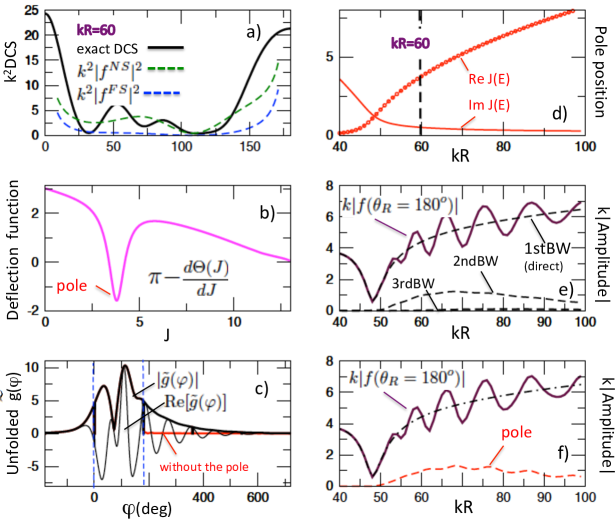
(a)

Figure 8: Example 2: the hard-sphere model (type II).
The task: to determine the origin of the backward scattering oscillations in Figure 1b).
(a) The full DCS (solid) and its NS and FS components (11)-(12) at $kR=60$. Thus, the presence of both components suggests that the oscillatory behaviour of the DCS is a NS-FS interference effect.
(b) The deflection function (25) at $kR=60$ exhibits a narrow dip. Thus, this suggests the presence of a single resonance Regge pole. The particle may be trapped in a metastable intermediate state at the total angular momentum $J\approx 4$.
(c) The unfolded amplitude $\tilde{g}(\varphi)$ at $kR=60$ extends beyond the first NS zone, $0<\varphi<\pi$ into the first FS and the second NS zone. Also shown (in red) is the result of subtracting from $\tilde{g}(\varphi)$ the ”exponential tail”, $\tilde{g}^{tail}(\varphi)$ associated with the Regge pole [cf. (d)]. Thus, for $\varphi>\pi$, one has an exponential decay of a single metastable state. The decay rate is such that the trapped particle can escape into the backward direction after one full rotation. This process is likely to interfere with the direct backward scattering resulting from a ”head-on collision” at $J\approx 0$.
(d) Real (circles) and imaginary (solid) parts of the Regge pole positions as functions of the particle’s energy. Thus, a single resonance affects the scattering shown in Figure 1b) in the energy range $55\lesssim kR\leq 100$.
(e) The backward scattering amplitude vs. energy. Also shown (dashed lines) are the backward scattering sub-amplitudes in Eq.(20), $f_{\nu{{}^{\prime}}\leftarrow\nu}(\theta_{R}=\pi,E|M)$, $M=0,1,2$. Thus, the probable cause of the oscillations in the DCS at $\theta_{R}=\pi$ for $kR>55$ is the interference between the scenarios where the particle bounces back immediately, or completes a single full rotation around the potential’s core. For $kR<55$, the resonance is short-lived, and the second scenario cannot be realised.
(f) Contribution of the resonance in (d) to backward scattering, as given by the second term in Eq.(31) (dashed). Also shown by a dot-dashed line is the result of subtracting it from the $f_{\nu{{}^{\prime}}\leftarrow\nu}(\theta_{R}=\pi)$.
Conclusion: As expected, the oscillations in the backward DCS [cf.(e),(f)] result from the interference between the rapid direct recoil and the decay of a trapped particle, after completing one full rotation.

(a)

Figure 9: Example 3: the $F+H_{2}(0,0,0)\to HF(2,0,0)+H$ reaction.
The task: to determine the origin of the forward scattering peak in Figure 1c).
(a) The full DCS (solid) and its NS and FS components (11)-(12) ( dashed) at the collision energy $E=32.27$ $meV$. Thus, the oscillatory pattern is likely to be a nearside-farside effect.
(b) The deflection function (25) at $E=32.27$ $meV$ exhibits two dips separated by a sharp peak. Thus, resonance effects are likely to play an important role.
(c) The unfolded amplitude $\tilde{g}(\varphi)$ at $E=32.27$ $meV$ extends beyond the first NS zone, $\varphi>\pi$. Also shown (in red and blue) the results of subtracting from $\tilde{g}(\varphi)$ the ”exponential tails”, $\tilde{g}^{(tail)}_{II}(\varphi)$ and $\tilde{g}^{(tail)}_{I}(\varphi)$, in (27), associated with the two Regge poles, labelled $I$ and $II$ in ${\bf(d)}$ (we follow the notations of [40]). Thus, forward scattering at $\theta_{R}=0$ occurs mostly via capture into intermediate states. There is a pair of such states involved.
(d) Real (circles) and imaginary (solid) parts of the Regge pole positions as functions of collision energy. Also shown (in green) are the real (crosses) and imaginary (solid) parts of the position of a Regge zero, responsible for the sharp peak in the deflection function in ${\bf(b)}$. Thus, both resonances are likely to affect the DCS in the entire energy range $27-50$ $meV$. The first state ($I$) becomes ever more long-lived as the energy increases, while the opposite happens to the state $II$.
(e) The forward scattering amplitude (solid) as a function of collision energy. Also shown by the dashed lines are the forward scattering sub-amplitudes in Eq.(19), $f^{FW}_{{\nu{{}^{\prime}}\leftarrow\nu}}(E|M)$, $M=0,1,2$. Thus, the structure in the DCD at $\theta_{R}=0$ for $E>37$ $meV$ is likely to result from the formation of an intermediate triatomic, which can return to the forward direction after up to two complete rotations.
(f) The exact forward scattering amplitude (solid), and the contributions of the two resonances ${\bf(d)}$, shown by dashed lines, as given by Eq.(32). Also shown (green, dashed) is the coherent sum of the two contributions.
Conclusion: The forward scattering peak at $E\approx 32-33$ $meV$ is caused by constructive interference between the decays of the resonances $I$ and $II$ into the first forward zone [40].

7 Summary

In summary, we present a user friendly computer code which evaluates the contribution a resonance Regge trajectory makes to a reactive differential cross section. Regge poles positions and residues are calculated using numerical values of the corresponding scattering matrix element by Padé reconstruction. The code can be used for analysing reactive transitions with zero initial and final helicity quantum numbers.

8 Acknowledgements:

We acknowledge support of the Basque Government (BERC 2018e2021 Program, Grant No. IT986-16, and ELKARTEK grants KK-2020/00049, KK-2020/00008), and MINECO, the Ministry of Science and Innovation of Spain (BCAM Severo Ochoa accreditation SEV-2017-0718 and Grants PGC2018-101355-B-100(MCIU/AEI/FEDER,UE, PID2019-104927GB-C22). This work has been possible thanks to the support of the computing infrastructure of the i2BASQUE academic network, DIPC Computer Center and the technical and human support provided by IZO- SGI SGIker of UPV/EHU and European funding (ERDF and ESF).

9 Appendix A: Example of DCS_Regge parameter file INPUT

(a)

Figure 10: An example of the INPUT file.

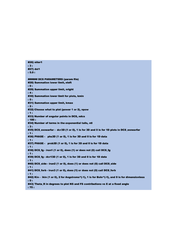
(a)

Figure 11: An example of the INPUT file (continued).

See Figure 10 and Figure 11.

10 Appendix B: Example of DCS_Regge input file 20

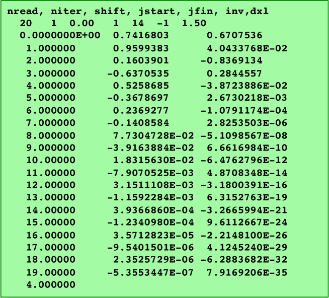
(a)

Figure 12: The input file 20, which contains the input parameters required to run Padé_II, the values of the $S$-matrix element for different values of $J$, and the value of collision energy in $meV$.

.

The contents of the file, also described in [53], include:
nread: the number of partial waves read,
niter: the number of iterations to remove the quadratic phase,
sht: this shifts the input grid points and may be used to avoid exponentiation of extremely large number when evaluating the polynomials involved. The value sht = nread$/2$ is suggested for a large number of partial waves.
jstart and jfin: with all input points numbered by j between 1 and N, determine a range jstart $\leq j\leq$ jfin to be used for the Padé reconstruction.
inv: set to $-1$, not used in present calculations,
dxl: determines the width of the strip in which poles and zeroes are removed while evaluating the quadratic phase in Eq. (11). See Figure 12.

11 Appendix C: Structure of the DCS directory

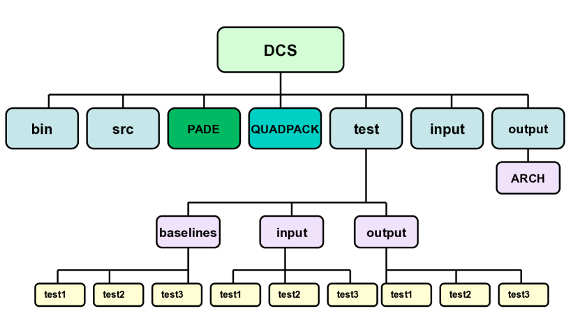
(a)

Figure 13: Detailed structure of the DCS directory.

See Figure 13.

12 Appendix D: Structure of the PADE directory

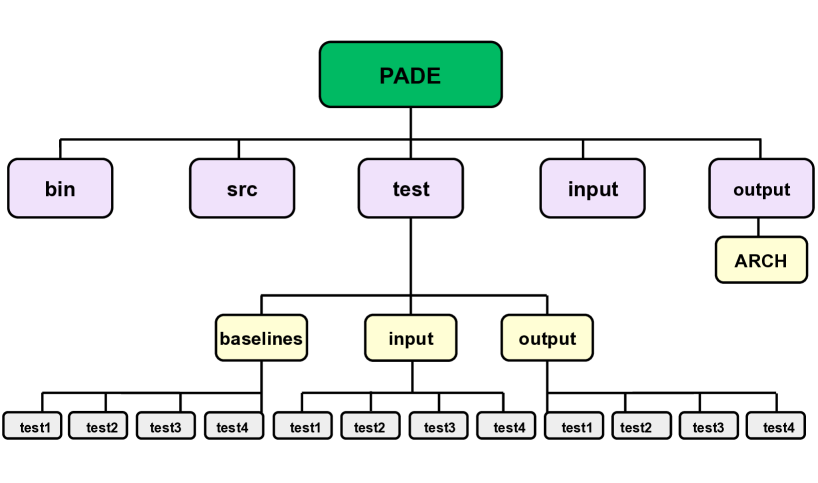
(a)

Figure 14: Detailed structure of the PADE directory.

See Figure 14.

13 Appendix E: Structure of the QUADPACK directory

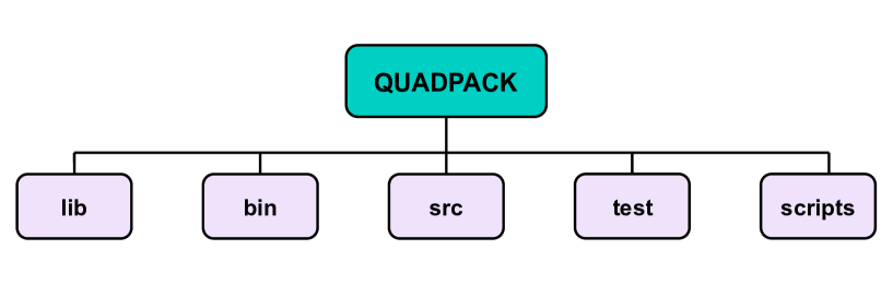
(a)

Figure 15: Detailed structure of the QUADPACK directory.

See Figure 15.

References

- [1] S.A. Harich, D.X. Dai, C.C. Wang, X. Wang, S.D. Chao and R.T. Skodje, Nature, 419, (2002) 281.
- [2] D.C. Clary, Quantum Theory of Reaction Dynamics, Science, 279 (1998) 1879.
- [3] D. Skouteris, D.E. Manolopoulos, W. Bian, H-J Werner, L-H Lai and K. Liu, Science, 286 (1999) 1713.
- [4] P. Casavecchia, N. Balucani and G.G. Volpi, Ann. Rev. Phys. Chem., 50 (1999) 347.
- [5] W.H. Miller, Adv. Chem. Phys., 25 (1974) 69.
- [6] D. Skouteris, J.F. Castillo and D.E. Manolopoulos, Comp. Phys. Commun., 133 (2000) 128.
- [7] S.C. Althorpe, F. Fernández-Alonso, B.D. Bean, J.D. Ayers, A.E. Pomerantz, R.N. Zare and E. Wrede, Nature, 416 (2002) 67.
- [8] V. Aquilanti, S. Cavalli and D. De Fazio, J. Chem. Phys., 109 (1998) 3792.
- [9] V. Aquilanti, S. Cavalli, A. Simoni, A. Aguilar, J.M. Lucas and D. De Fazio, J. Chem. Phys., 121 (2004) 11675.
- [10] V. Aquilanti, S. Cavalli, D. De Fazio, A. Volpi, A. Aguilar, X. Giménez and J.M. Lucas, Phys. Chem. Chem. Phys., 4 401 (2002).
- [11] J.N.L. Connor, J. Chem. Soc. Faraday Trans., 305 (1990) 1627.
- [12] P.G. Burke and C. Tate, Comput. Phys. Commun., 1 (1969) 97.
- [13] D. Sokolovski, Phys. Rev. A., 62 (2000) 024702-01.
- [14] D. Sokolovski, A.Z. Msezane, Z. Felfli, S.Yu. Ovchinnikov and J.H. Macek, Nuclear Instruments and Methods in Physics Research Section B: Beam Interactions with Materials and Atoms, 261 (2007) 133.
-
[15]
D. Sokolovski and E. Akhmatskaya, Phys. Lett. A, 375 (2011) 3062.
Please note that there is a typo in Eq.(5), which should read
with and . This regrettable misprint does not, however, affect the results or conclusions of the paper, as the correct values have been used in all calculations. - [16] D. Sokolovski, Z. Felfli and A.Z. Msezane, Self-intersecting Regge trajectories in multi-channel scattering, Phys. Lett. A, 376 (2012) 733.
- [17] J.N.L. Connor, Chemical Society Reviews, 5 (1976) 125.
- [18] J.N.L. Connor, W. Jakubetz and C.V. Sukumar, J. Phys. B, 9 (1976) 1783.
- [19] J.N.L. Connor and W. Jakubetz, Mol. Phys., 35 (1978) 949.
- [20] J.N.L. Connor, D.C. Mackay and C.V. Sukumar, J. Phys. B, 12 (1979) L5151.
- [21] J.N.L.Connor, in ”Semiclassical methods in molecular scattering and spectroscopy.” Proceedings of the NATO Advanced Study Institute held in Cambridge, England, in September, 1979. Edited by M.S. Child. Reidel, Dordrecht, The Netherlands, (1980) 45.
- [22] J.N.L. Connor, D. Farrelly and D.C. Mackay, J. Chem. Phys., 74 (1981) 3278.
- [23] K.-E. Thylwe and J.N.L. Connor, J. Phys. A, 18 (1985) 2957.
- [24] J.N.L. Connor, D.C. Mackay and K.-E. Thylwe, J. Chem. Phys., 85 (1986) 6368.
- [25] D. Bessis, A. Haffad and A.Z. Msezane, Phys. Rev. A., 49 (1994) 3366.
- [26] J.N.L. Connor and K.-E. Thylwe, J. Chem. Phys., 86 (1987) 188.
- [27] P. McCabe, J.N.L. Connor and K.-E. Thylwe, J. Chem. Phys., 98 (1993) 2947.
- [28] D. Sokolovski, J.N.L. Connor and G.C. Schatz, Chem. Phys. Lett., 238 (1995) 127.
- [29] D. Sokolovski, J.N.L. Connor and G.C. Schatz, J. Chem. Phys., 103 (1995) 5979.
- [30] P. McCabe and J.N.L. Connor, J. Chem.Phys , 104 (1996) 2297.
- [31] D. Sokolovski, J.F. Castillo and C. Tully, Chem. Phys. Lett., 313 (1999) 225.
- [32] D. Sokolovski and J.N.L. Connor, Chem. Phys. Lett., 305 (1999) 238.
- [33] A.J. Dobbyn, P. McCabe, J.N.L. Connor and J.F. Castillo, Phys. Chem. Chem. Phys., 1 (1999) 1115.
- [34] P. McCabe, J.N.L. Connor and D. Sokolovski, J.Chem.Phys , 114 (2001) 5194.
- [35] D. Sokolovski and J.F. Castillo, Phys. Chem. Chem. Phys., 2 (2000) 507.
- [36] F.J. Aoiz, L. Bañares, J.F. Castillo and D. Sokolovski, J. Chem. Phys., 117 (2002) 2546.
- [37] D. Sokolovski, 370 (2003) 805.
- [38] D. Sokolovski and A.Z. Msezane, Phys. Rev. A., 70 (2004) 032710.
- [39] D. Sokolovski, S.K. Sen, V. Aquilanti, S. Cavalli and D. De Fazio, J. Chem. Phys., 126 (2007) 084305.
- [40] D. Sokolovski, D. De Fazio, S. Cavalli and V. Aquilanti, Phys. Chem. Chem. Phys., 9 (2007) 5664.
- [41] J.N.L. Connor, J. Chem. Phys., 138 (2013) 124310.
- [42] C. Xiahou, J.N.L. Connor and D.H. Zhang, Phys. Chem. Chem. Phys., 13 (2011) 12981.
- [43] X. Shan, C. Xiahou and J.N.L. Connor, Phys. Chem. Chem. Phys., 20 (2018) 819.
- [44] C. Xiahou, X. Shan and J.N.L. Connor, Phys. Scr., 94 (2019) 065401.
- [45] X. Shan and J.N.L. Connor, J. Chem. Phys., 136 (2012) 044315.
- [46] X. Shan and J.N.L. Connor, J. Phys. Chem. A, 116 (2012) 11414.
- [47] X. Shan and J.N.L. Connor, J. Phys. Chem. A, 118 (2014) 6560.
- [48] M. Hankel and J.N.L. Connor, AIP Advances, 5 (2015) 077160.
- [49] X. Shan and J.N.L. Connor, J. Phys. Chem. A, 120 (2016) 6317.
- [50] C. Xiahou, X. Shan and J.N.L. Connor, J. Phys. Chem. A, 123 (2019) 10500.
- [51] G.A. Baker, Jr., The essentials of Padé Approximations, Academic, New York, 1975.
- [52] R. Piessens, E. de Doncker-Kapenga, C.Überhuber, D. Kahaner, QUADPACK, A Subroutine Package for Automatic Integration, Springer-Verlag (1983).
- [53] D. Sokolovski, E. Akhmatskaya and S.K. Sen, Comp. Phys. Comm., 182 (2011) 448.
- [54] A.R. Edmonds, Angular Momentum in Quantum Mechanics, 2nd edn., 3rd printing with corrections, Princeton University Press, Princeton, NJ, 1974.
- [55] D.M. Brink, Semiclassical Methods in Nucleus-Nucleus Scattering, Cambridge University Press, Cambridge, 1985.
- [56] E. Akhmatskaya, D. Sokolovski and C. Echeverría-Arrondo, Comp. Phys. Comm., 185 (2014) 2127.
- [57] D. Sokolovski, E. Akhmatskaya, C. Echeverría-Arrondo and D. De Fazio, Phys. Chem. Chem. Phys., 17 (2015) 18577.
- [58] R.P. Feynman, R. Leighton and M. Sands, The Feynman Lectures on Physics III (Dover Publications, Inc., New York, 1989), Ch.1: Quantum Behavior.
- [59] E. de Doncker-Kapenga, ACM SIGNUM Newsl., 13 (2) (1978) 12-18.
- [60] P. Wynn, Math. Tables Aids Comput., 10 (1956) 91-96.
- [61] D. Vrinceanu, A.Z. Msezane, D. Bessis, J.N.L. Connor and D. Sokolovski, Chem. Phys. Lett., 324 (2000) 311.
- [62] D. Sokolovski and S. Sen, in Semiclassical and other Methods for Understanding Molecular Collisions and Chemical reactions, Collaborative Computational Project on Molecular Quantum Dynamics (CCP6), Ed. by S.K. Sen, D. Sokolovski and J.N.L. Connor, Daresbury, UK (2005) 104.