globalization_mechanism \BODY \NewEnvironglobalization_strategy \BODY \NewEnvironstep_computation \BODY
Binary Control Pulse Optimization for Quantum Systems
Abstract
Quantum control aims to manipulate quantum systems toward specific quantum states or desired operations. Designing highly accurate and effective control steps is vitally important to various quantum applications, including energy minimization and circuit compilation. In this paper we focus on discrete binary quantum control problems and apply different optimization algorithms and techniques to improve computational efficiency and solution quality. Specifically, we develop a generic model and extend it in several ways. We introduce a squared -penalty function to handle additional side constraints, to model requirements such as allowing at most one control to be active. We introduce a total variation (TV) regularizer to reduce the number of switches in the control. We modify the popular gradient ascent pulse engineering (GRAPE) algorithm, develop a new alternating direction method of multipliers (ADMM) algorithm to solve the continuous relaxation of the penalized model, and then apply rounding techniques to obtain binary control solutions. We propose a modified trust-region method to further improve the solutions. Our algorithms can obtain high-quality control results, as demonstrated by numerical studies on diverse quantum control examples.
1 Introduction
Quantum control [1, 2, 3] is a rich field that started with applications in quantum chemistry [4, 5, 6, 7, 8] but has since expanded to other subfields such as atomic, molecular, and optical physics [9, 10, 11]. Quantum control theory has been used in the quantum information community for a long time, mostly for designing pulse controls and gates in quantum devices [12, 13, 14, 15, 16, 17, 18, 19, 20]; but more recently, researchers have considered using control theories and optimization for the high-level design of quantum algorithms [21, 22, 23, 24, 25, 26, 27]. In this paper, we focus primarily on the quantum information applications of control theory, but our methods are generalizable to other settings. We do not focus on the analytic aspects of quantum control but on the more mechanistic aspects of how to apply optimization techniques to the problem of designing and finding solutions to a variety of quantum control problems.
Quantum computing architecture falls into different categories, such as quantum circuits, which utilize discrete unitary gates to control a system, and quantum annealing [28, 29], which uses smooth Hamiltonian evolution instead. Quantum control is already familiar within quantum circuit architecture design as a method for designing quantum gates, and several of our examples described in Section 2 belong to this category. Within the framework of quantum algorithms, quantum control is often used in variational quantum algorithms, which can straddle the line between discrete gates and smooth evolution. This paper focuses mainly on discrete binary control, which is more applicable to a quantum gate architecture. Variational techniques have already been implemented experimentally (see, e.g., [30, 31]), and our techniques can potentially enhance the performance of the classical variational loop on such near-term devices.
Most quantum optimal control algorithms are based on gradient descent for better convergence than using gradient-free algorithms [32]. Khaneja et al. [9] proposed the gradient ascent pulse engineering (GRAPE) algorithm for designing pulse sequences in nuclear magnetic resonance. The authors approximated the control function by a piecewise-constant function and evaluated the explicit derivative. Based on the GRAPE algorithm, Larocca and Wisniacki [33] proposed a K-GRAPE algorithm by using a Krylov subspace to estimate quantum states during the process of time evolution. Brady et al. [25] applied an analytical framework based on gradient descent to discuss the optimal control procedure of a special control problem that minimizes the energy of a quantum state with a combination of two Hamiltonians. Another class of quantum optimal control algorithms is based on the chopped random basis (CRAB) optimal control technique, which describes the control space by a series of basis functions and optimizes the corresponding coefficients [34, 35]. Sørensen et al. [36] combined the GRAPE algorithm and CRAB algorithm to achieve better results and faster convergence. However, all these algorithms are designed for unconstrained continuous quantum control problems.
In this work, we focus on a quantum pulse optimization problem having binary control variables and restricted feasible regions derived by linear constraints. These constraints describe a so-called bang-bang control in a model that corresponds to a quantum circuit design similar to that in the quantum approximate optimization algorithm (QAOA) [37] and other variational quantum algorithms [38, 39]. Some literature formulates the QAOA algorithm into bang-bang control problems with a fixed evolution time and investigates the performance of multiple methods including Stochastic Descent and Pontryagin’s minimum principle for optimizing control models [40, 41]. However, they only consider quantum systems with two controllers, while we propose a more general solution framework for quantum systems with multiple controllers. In this paper, we introduce four quantum control examples: (i) energy minimization problem, (ii) controlled NOT (CNOT) gate estimation problem, (iii) NOT gate estimation problem with the energy leakage, and (iv) circuit compilation problem. The nonconvexity, binary variables, and restricted feasible sets in these examples lead to extreme challenges and difficulties in solving the related binary quantum control problems.
Methods for binary control mainly include genetic algorithms [42], branch-and-bound [43, 44], and local search [45]. To the best of our knowledge, genetic algorithms have not been applied to binary quantum control, but Zahedinejad et al. [46] showed that such algorithms fail to obtain high-quality solutions even to continuous quantum control problems. Branch-and-bound can find high-quality solutions for binary optimal control, but the long computational time makes the algorithm intractable and hard to use for large-scale practical problems. Vogt and Petersson [45] introduced a trust-region method [32] to solve the single flux quantum control problem with binary controls. We extend their approach by allowing the addition of constraints, such as min-up-time and max-switching constraints to control the number of switches.
The main contributions of this paper are as follows. First, we propose a generic model including continuous and discretized versions for binary quantum control problems with linear constraints indicating that at each time step there can be only one active control. Second, we introduce an exact penalty function for linear constraints and develop an algorithmic framework combining the GRAPE algorithm and rounding techniques to solve it. Third, to prevent chattering on controls, we propose a new model that includes a total variation (TV) regularizer, and then we propose a new approach based on the alternating direction method of multipliers (ADMM) to solve this model. Fourth, we introduce a modified trust-region method to improve the solutions obtained from these algorithms. Compared with other methods, our algorithmic framework can obtain high-quality binary control sequences and prevent frequent switches. We demonstrate the performance on multiple quantum control examples with various objective functions and controllers.
The paper is organized as follows. In Section 2 we construct generic models of quantum binary control problems using continuous and discretized formulations. We also introduce the corresponding specific formulations for four quantum control examples. In Section 3 we review the GRAPE algorithm, utilize a penalty function to relax certain linear constraints, and introduce our rounding techniques. In Section 4 we propose and solve the penalty model with the TV regularizer and the corresponding ADMM algorithm. In Section 5 we derive trust-region subproblems and propose an approximate local-branching method based on the trust-region algorithm. In Section 6 we present numerical simulations for multiple instances of the three quantum control examples in Section 2 to demonstrate the computational efficacy and solution performance of our models and algorithms. In Section 7 we summarize our work and propose future research directions.
2 Formulations for Quantum Control
Consider a quantum system with qubits and a time horizon , where is defined as the evolution time. Let be the intrinsic Hamiltonian. Let be the number of control operators and be the given control Hamiltonians. Let be the initial and target unitary operators of the quantum system, respectively. Define variables as the real-valued control functions at time , and use to represent the corresponding vector form. Define variables as the time-dependent control Hamiltonian function and as the time-dependent unitary quantum operator function. A generic quantum control problem for optimizing a function of quantum operators is formulated as
| (1a) | ||||
| s.t. | (1b) | |||
| (1c) | ||||
| (1d) | ||||
| (1e) | ||||
| (1f) | ||||
The objective function (1a) is a general function with respect to the final unitary operator . We assume that is a differentiable function. In Sections 2.1–2.4, we provide the specific formulations of the objective function for four quantum control examples. Constraint (1b) describes the computation of the time-dependent Hamiltonian function based on the intrinsic Hamiltonian, control Hamiltonians, and control functions. Constraint (1c) is the ordinary differential equation describing the time evolution of the operator of the quantum system with the same units for energy and frequency, setting . Constraint (1d) is the initial condition of the operator. Constraint (1e) indicates that the summation of all the control functions should be one at all times, which is described by the Special Ordered Set of Type 1 (SOS1) property in optimal control theory [47]. In binary control, this SOS1 property guarantees that only one control field will be active at a time that mimics the bang-bang nature of some quantum applications such as the quantum approximate optimization algorithm and the variational quantum eigensolver (VQE). Constraints (1f) require all time-based values of the control functions to be feasible.
Following the time discretization process in [9], we explicitly integrate constraint (1c). In particular, we divide the time horizon into time intervals . We consider time intervals with an equal length represented by , but our work readily extends to nonuniform discretizations. For each controller and each time step , we define discretized binary control variables as . For each time step , we define the discretized time-dependent Hamiltonians as and the quantum operators as . The differential equation (1c) is thus approximated by
| (2) |
For each , the linear differential equation (2) is a Schrödinger equation of a unitary operator, and we obtain an explicit solution as
because is time independent. We then obtain a discretized quantum control problem (DQCP) as a discretization of the differential control model (1) using explicit solutions on each interval for unitary operators as
| (3a) | ||||
| s.t. | (3b) | |||
| (3c) | ||||
| (3d) | ||||
| (3e) | ||||
| (3f) | ||||
The objective function (3a) is the objective function (1a) evaluated at the approximated final operator . Constraints (3b)–(3f) are the discretized formulations of constraints (1b)–(1f). In the following sections we use this discretized formulation to develop our algorithms. We present the following discussion on the relationship between the continuous and discretized formulation.
Remark 1.
Remark 2.
The model can be generalized to instances with multiple active controllers in any time interval by considering each possible combination of the controllers. For an instance with control Hamiltonians , we consider combinations and define control functions for each combination. Thus, the original problem is converted to a new problem with only one active controller in any time interval.
In our paper we consider four examples with different objective functions and control Hamiltonians. In the following sections we introduce the continuous model of four example problems in quantum control. They can be formulated as discretized models (3) following the above discretization process.
2.1 Energy Minimization Problem
Consider a quantum spin system consisting of qubits, no intrinsic Hamiltonian, and two control Hamiltonians . The initial operator is a -dimensional identity matrix. Let be the ground state of the first control Hamiltonian . The ground state energy of this quantum system is the minimum eigenvalue of the control Hamiltonian , represented by in our model. Since the ground state energy differs across problem instances, it is important to compare performance consistently across these instances. Therefore, we maximize the approximation ratio, defined as the achieved energy divided by the true ground state energy. The problems we study are well defined so that the initial state of the system has zero energy with respect to ; furthermore, the ground state energy will always be a large negative number. Therefore, the approximation ratio reflects the energy level achieved by our procedure from the initial energy of zero to the true ground state energy. Because our procedure can improve the state relative only to its initial configuration, a negative approximation ratio is not possible.
To ensure consistency with the objective functions of our other two examples, we minimize one minus the approximation ratio. Because the true ground state energy is negative, this formula is equivalent to minimizing the achieved energy. The continuous-time formulation is
| (5a) | ||||
| s.t. | (5b) | |||
| (5c) | ||||
| Constraints (1c)–(1e) | ||||
| (5d) | ||||
where represents the conjugate transpose of a matrix and represents the conjugate transpose of a quantum state vector . The matrix is the adjacency matrix of a randomly generated graph with nodes, and are Pauli matrices of qubit .
2.2 CNOT Gate Estimation Problem
Our second example is defined on an isotropic Heisenberg spin-1/2 chain with length 2 according to [48]. For our study we consider just the unitary evolution with no energy leakage. The quantum system includes 2 qubits, an intrinsic Hamiltonian , and two control Hamiltonians . The initial operator is a -dimensional identity matrix and the target operator is the matrix formulation of the CNOT gate represented by . This problem’s continuous-time formulation is
| (6a) | ||||
| s.t. | (6b) | |||
| (6c) | ||||
| (6d) | ||||
| Constraints (1c)–(1d) | ||||
| (6e) | ||||
where are Pauli matrices of two qubits. The goal is to minimize the objective function, defined as the infidelity between the final operator and the target operator.
2.3 NOT Gate Estimation with Energy Leakage
We consider an anharmonic multilevel system that is widely used in quantum experiments to implement physical qubits. Following [49], we consider the lowest three levels of an energy spectrum with only nearest-level coupling for a single qubit . The first two levels comprise the qubit and the third level models the energy leakage. Under this setting, the system contains an intrinsic Hamiltonian and two control Hamiltonians . The initial operator is a 3-dimensional identity matrix, and the target operator is the matrix formulation of the NOT gate corresponding to the lowest three levels of the energy spectrum represented by , which is
| (7) |
The continuous-time formulation of this problem is
| (8a) | ||||
| s.t. | (8b) | |||
| (8c) | ||||
| (8d) | ||||
| (8e) | ||||
| Constraints (1c)–(1d) | ||||
| (8f) | ||||
where represents a vector with the -th element as 1 and other elements as 0. The parameters weigh the relative strength of transitions and the parameters correspond to the drive frequency. We present the specific values of the parameters used in numerical simulations in Section 6.2.
2.4 Circuit Compilation Problem
For a general quantum algorithm, each quantum circuit needs to be compiled to a representation imposed by specific controllers and constraints in order to execute the algorithm on specific quantum devices. We take quantum circuits generated by the unitary coupled-cluster single-double (UCCSD) method [50, 51] for estimating the ground state energy of molecules in quantum chemistry as examples. We consider the Hamiltonian controllers in the gmon-qubit system [52] with qubits. Each qubit has a flux-drive controller and a charge-drive controller. In addition, there is a rectangular-grid topology with nearest-neighbor connectivity denoted by , and each pair of connected qubits has a controller. Define as control functions for the connected qubits controllers and use to represent the corresponding vector form of . The initial operator is a -dimensional identity matrix. The target operator is the matrix formulation of the quantum circuit generated by UCCSD for specific molecules represented by . We refer interested readers to Gokhale et al. [53] for more details. The continuous-time formulation of this problem is
| (9a) | ||||
| s.t. | (9b) | |||
| (9c) | ||||
| (9f) | ||||
| (9g) | ||||
| Constraints (1c)–(1e) | ||||
| (9h) | ||||
where are parameters corresponding to the quantum system and is the Pauli matrix of qubit . We finish this section by showing a general property of the objective function in optimal control problems.
Theorem 1.
Proof.
By definition, the objective function value cannot be larger than . From the definition of our quantum control problem, the quantum operators and are both unitary matrices. Therefore, we can write as , where are the orthonormal column vectors of and are vectors with the th component as and all the other components as . Thus we have
| (10) |
The first inequality follows from the fact that the trace of a product is invariant under cyclic permutations of the factors. The second inequality follows from . As a result, the objective function is no less than , and this completes the proof. ∎
Remark 3.
All the problems in this section fall into a class known as right-invariant systems [54] that consists of control problems on Lie groups. Specifically, this class consists of all control problems described by a Hamiltonian of the form . Controllability results on this class of control problems are well known [54, 55]. A test of controllability of these problems consists of examining the dynamical Lie algebra generated by the Hamiltonians, , and their nested commutators and comparing that Lie algebra with the Lie algebra of the subgroup defined by the symmetries in a given problem. For the systems considered in this paper, there are indeed enough control Hamiltonians to reach the target state by using piecewise continuous control functions, .
3 Binary Quantum Control Algorithms
In this section we propose models and algorithms to obtain binary quantum control results for the discretized model (3). In Section 3.1 we review the adjoint approximation method of gradients used in the GRAPE algorithm for solving the continuous relaxation of the optimal control problem (3) and derive the gradient update rule for the aforementioned four specific examples. In Section 3.2 we propose an exact penalty function for the SOS1 property that allows us to add constraints to GRAPE. In Section 3.3 we introduce rounding techniques to obtain binary controls. These algorithms form the basis of our discrete framework discussed in Sections 4–5.
The overall framework is outlined in Figure 1, which presents the methods in Sections 3–5 and the corresponding tables and results. We summarize the algorithms of our framework in Table 1. In the figure, the rectangles represent the three formulations of our model, and the ellipses represent the algorithms. The parallelograms show the result tables corresponding to algorithms, where the dashed parallelograms refer to the results of the continuous models and the solid parallelograms refer to the results of the discrete models.
Name Algorithms pGRAPE Solving the continuous relaxation with squared -penalty function by penalized GRAPE. TR Solving the continuous relaxation with TV regularizer and SOS1 property by a trust-region method. ADMM Solving the continuous relaxation with TV regularizer and SOS1 property by ADMM. SUR Rounding the continuous solutions without hard control constraints. MT Rounding the continuous solutions with min-up-time constraints. MS Rounding the continuous solutions with max-switching constraints. ALB Improving the binary solutions by the approximate local-branching method.
3.1 GRAPE Approach for Solving Continuous Relaxations
The GRAPE algorithm [9] is a gradient descent algorithm for solving the unconstrained continuous control problem. We derive a gradient descent algorithm based on the adjoint approach used in the GRAPE algorithm to solve the continuous relaxation of our discretized model (3) without the SOS1 property enforced by constraint (3e). We eliminate variables and by converting them into implicit functions of the control variables using constraints (3b)–(3d). Then the minimization problem of on is converted to the minimization problem of over the variables . The goal of the adjoint approach is to approximate the gradient of the objective function with respect to control variables based on the discretized time horizon. For simplicity, we define propagators for each time step as . For small , the gradient of corresponding to is estimated as
| (11) |
The gradient of the objective function with respect to the propagators depends on its specific formulation. We discuss gradients of two specific functions for the examples in Section 2.
Energy function
For generality, we use to represent the Hamiltonian in the energy objective function, which means that the goal is to minimize the energy corresponding to . Specifically, we have in the example in Section 2.1. The general energy function can be expressed as
| (12) |
For each time step , define variables . For the last time step , we define a variable . Then the gradient with respect to is computed as
| (13) |
Infidelity function
The infidelity function can be expressed as
| (14) |
For each time step , define variables . For the last time step , we define a variable . Then the gradient of the trace with respect to is computed as
| (15) |
Using the definition of objective function , we compute the gradient as
| (16) |
where represents the argument of a complex number.
With these computed gradients, we minimize the reduced function with respect to control variables by L-BFGS-B [56], a well-known quasi-Newton algorithm for solving bound-constrained optimization problems.
Remark 4.
Our implementation of GRAPE extends the classical gradient-ascend scheme (see, e.g., [9, 33]) in a number of ways: We use a bound-constrained quasi-Newton method to solve problems with bounded control variables, and we introduce a penalized GRAPE (denoted by pGRAPE) that adds a quadratic penalty of the SOS1 property in Section 3.2.
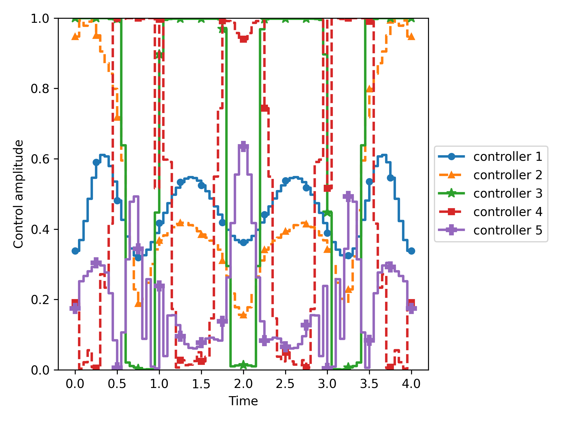
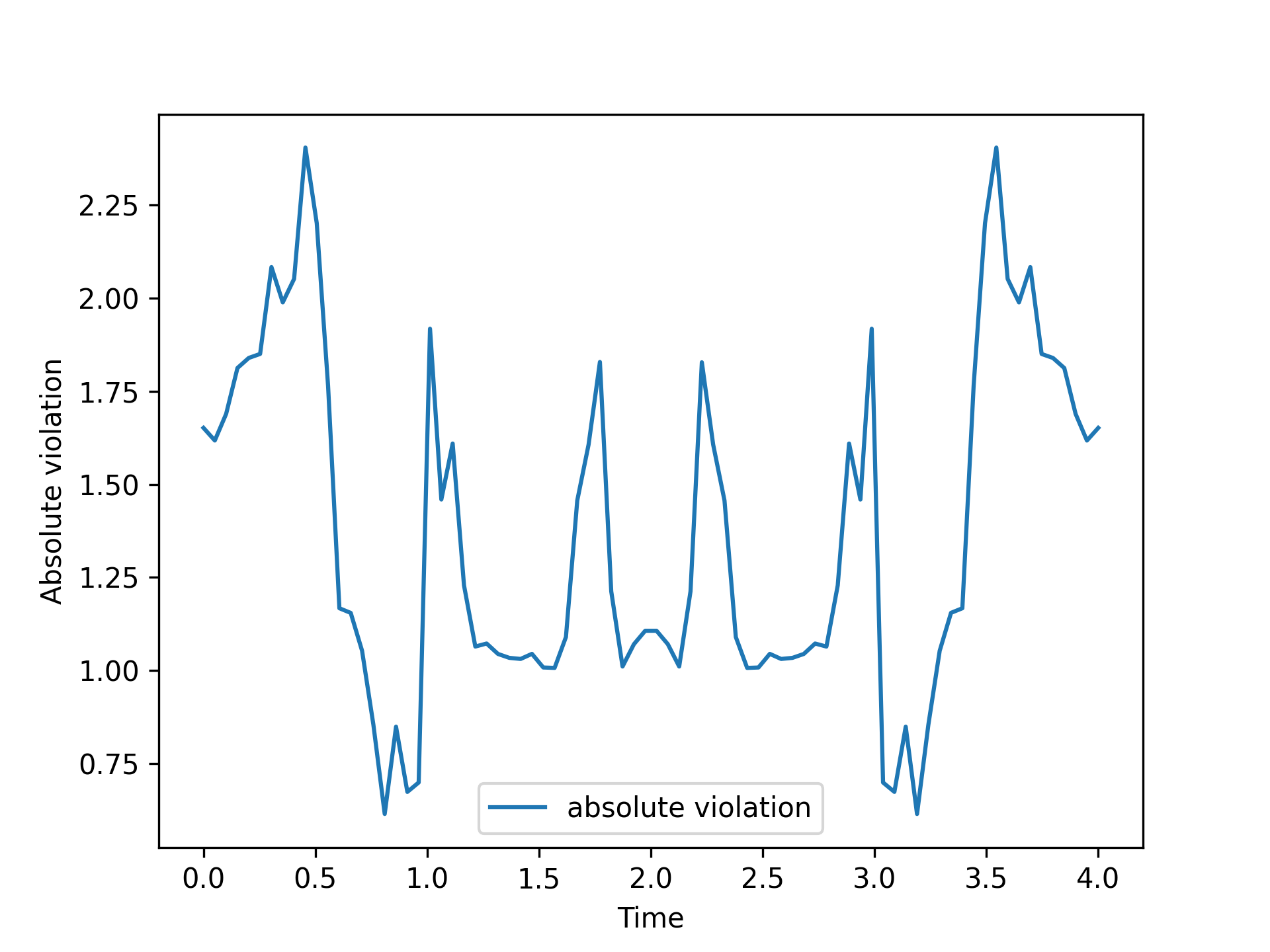
We take the circuit compilation problem (Section 2.4) on the molecule H2 (dihydrogen) as an example to show the control results, and we present the continuous control results without the SOS1 property obtained by the GRAPE algorithm in Figure 2a. We define the absolute violation of the SOS1 property at each time step as and present the value at each time step in Figure 2b. The figure shows that the results violate the SOS1 property at all time steps, with the maximum absolute violation being . Hence we introduce a penalized function in Section 3.2 to impose the SOS1 property.
3.2 Penalty Function for SOS1 Property
Our GRAPE algorithm is defined only for unconstrained or bound-constrained problems [9]. Hence, we convert the SOS1 property (3e) into a squared -penalty term and add it to the objective function. Define the squared function of the constraint violation as
| (17) |
We let a constant be the penalty parameter. Then the model with the penalty function is
We use to denote the optimized value of the squared function under the penalty parameter . The following theorem discusses the exactness of the penalized objective function.
Theorem 2.
A more general version of Theorem 2 is proved in [57]. Next we discuss the value of the optimized squared -penalty term with respect to the penalty parameter for the continuous relaxation of (3.2).
Theorem 3.
A detailed proof is provided in Appendix A.1.
Remark 5.
Remark 6.
For the quantum control problem with two controllers, the SOS1 can be enforced directly by substituting
| (18) |
in the model instead of using the penalty function.
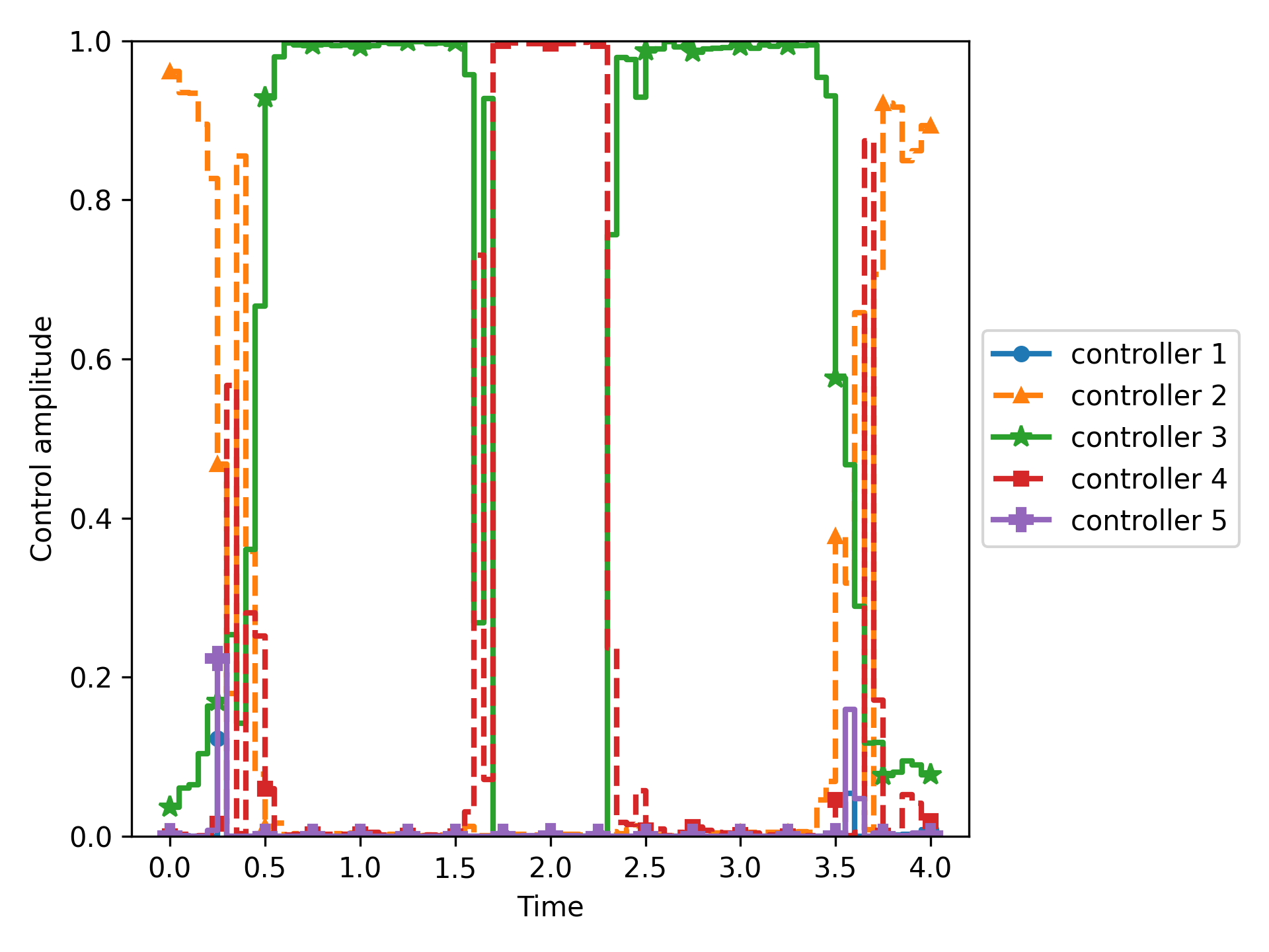
We show the control results obtained from the continuous relaxation with the squared -penalty function and penalty parameter in Figure 3. The value of the squared penalty term is , leading to a small error between continuous and binary results with the SOS1 property obtained by rounding techniques. However, we still need to provide rounding techniques to obtain binary results.
3.3 Rounding Techniques and Optimality Guarantees
In this section we introduce rounding techniques to obtain binary control results and investigate their optimality guarantees. In Section 3.3.1 we review the sum-up rounding technique designed for binary controls without constraints and discuss the difference compared with the continuous results. In Section 3.3.2 we introduce the integral minimization problem for rounding to obtain restricted binary controls.
3.3.1 Sum-Up Rounding
The sum-Up rounding (SUR) strategy proposed by Sager et al. [47] is a well-known method to obtain integer controls from continuous, relaxed ones in optimal control theory; see, for example, [58, 59]. One concern when applying SUR is that the solution of the relaxation does not satisfy the SOS1 constraints because the exactness of the squared -penalty is only for binary controls. We show that as long as the violation of the SOS1 constraint is small, the solution that is constructed via SUR still satisfies the strong convergence properties of SUR. We define the discretized continuous control function as . We define the discretized binary control function as . For each time step , we denote the vector form of control variables as and . We define the current cumulative deviation between continuous and binary controls as . The SUR approach to obtain binary controls is described in Algorithm 1.
The construction of ensures that the binary control satisfies the SOS1 property. Sager et al. [47] proved that if the continuous control satisfies the SOS1 property, then the rounded control will converge to when the length of a time interval converges to zero. This does not hold for arbitrary continuous controls without the SOS1 property, however, as the next proposition shows.
Proposition 1.
Let continuous control and binary control defined in Algorithm 1 be given for . Define
| (19) |
If , then satisfies the SOS1 property at any time step , and we have
| (20) |
The proof is provided in Appendix A.2. We have the following estimate of the difference between the continuous control without the SOS1 property and the rounded control.
Theorem 4.
With the same definition of in Proposition 1, it holds that for any time step ,
| (21) |
Because and are bounded, we have if . The proof of the inequality (21) extends the proof for Theorem 5 in [47]. We modify the right-hand side of the inequality by adding a term . We provide the detailed proof in Appendix A.2. In the following corollary we show that for our bounded discretized quantum control problem, converges to zero as converges to zero, ensuring the convergence of the rounded control to the continuous control.
Corollary 1.
Let be the value of the optimized squared term in the continuous relaxation of the model (3.2). Then it holds that
| (22) |
where is the evolution time. Furthermore, if the original objective function is bounded, the rounded control will converge to the continuous control when is small enough.
The proof is provided in Appendix A.2. Based on the convergence of binary results to continuous results, we present the following proposition to guarantee the optimality of binary results.
Proposition 2.
Under the discretized setting of the quantum control problem, let be the continuous control and be the binary control obtained by Algorithm 1. Then the state of time evolution with binary control converges to the state with continuous control at each time step, namely,
| (23) |
leading to for a continuous objective function.
The proof is provided in Appendix A.2.
3.3.2 Combinatorial Integral Approximation
To obtain discretized binary controls, Sager [60] proposed a more general rounding technique by minimizing the integral difference between continuous and binary controls with certain additional constraints on the binary controls called combinatorial integral approximation (CIA). Let be the feasible region for binary controls. For each controller and each time step , define and as the discretized continuous and binary controls. We use and to represent the corresponding vector forms. The optimization problem for rounding is formulated as a mixed-integer problem
| (24a) | ||||
| s.t. | (24b) | |||
The rounding optimization problem can be solved by diverse algorithms for solving integer programs. In this paper we choose a branch-and-cut algorithm [61]. Furthermore, the rounding result obtained from SUR is an optimal solution of model (24) with [60]. In practice, researchers and engineers have proposed diverse restrictions on binary controls to avoid frequent switches. We formulate two main types of constraints as linear constraints.
Min-Up-Time Constraints.
Let be the minimum number of steps that the controller is active. The min-up-time constraints enforce that each controller is active for at least time steps. The restricted feasible region is formulated by the following linear constraints:
| (25) |
Max-Switching Constraints.
Let be the maximum number of switches during the evolution time horizon . The max-switching constraints enforce an upper bound on the total number of switches for each controller. We describe the restricted feasible region by linear constraints as
| (26) |
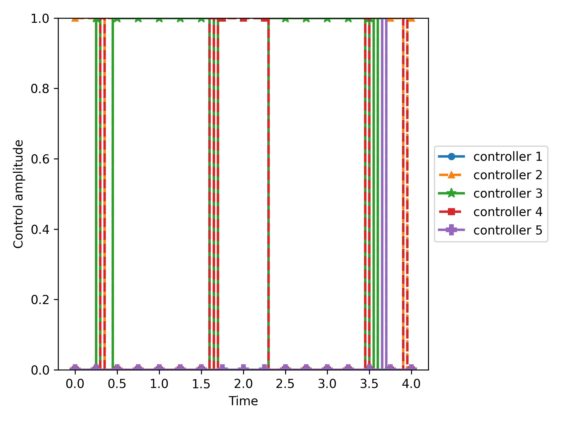
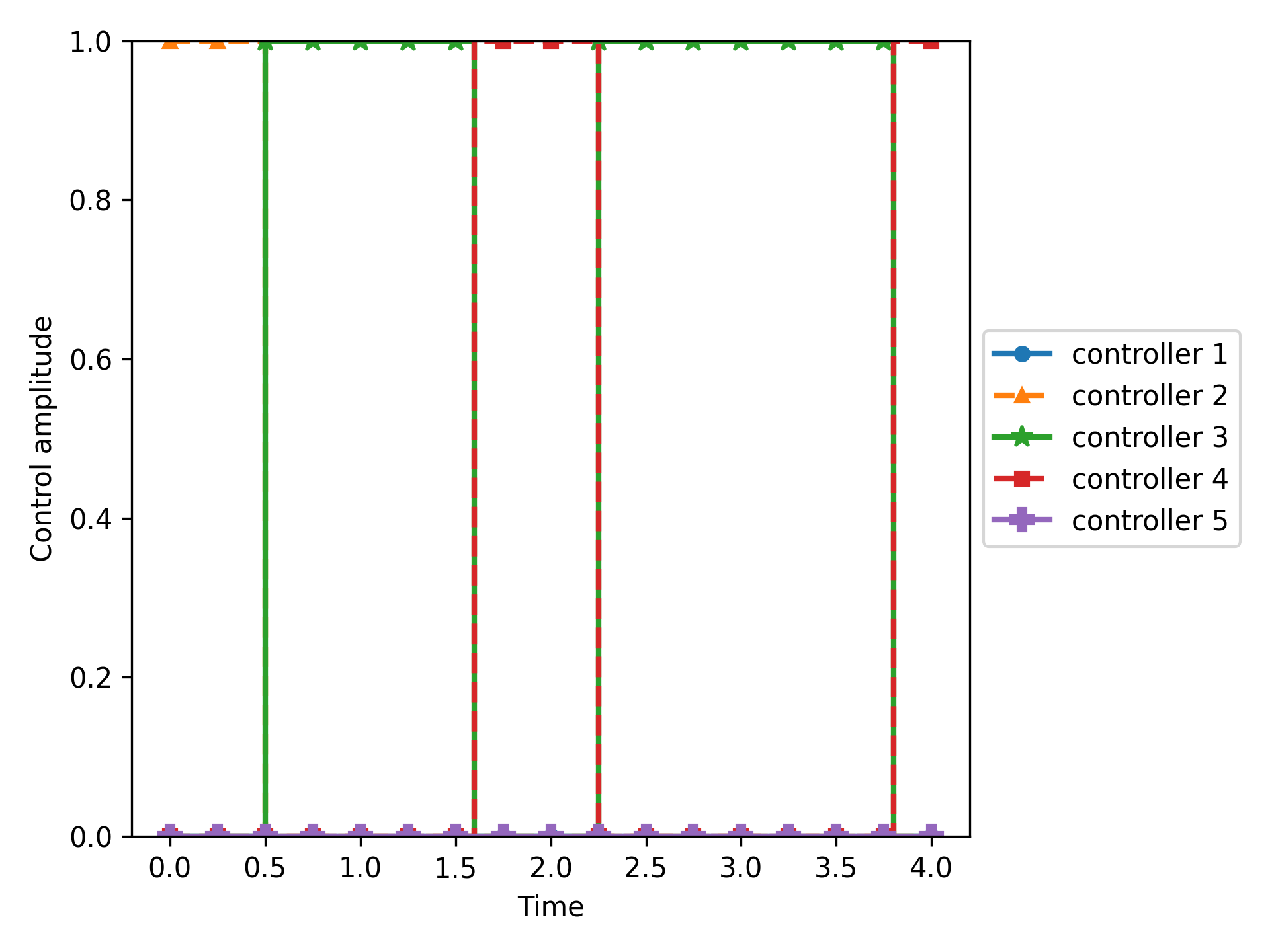
We present the binary results obtained from SUR and CIA with min-up-time constraints in Figure 4. We show that SUR leads to chattering on singular arcs. Although CIA can prevent frequent switches by setting hard constraints on the controls, it leads to a serious objective value increase. In Section 4 and Section 5 we propose models and algorithms to reduce switches when taking the original objective function into account.
4 Model with the TV Regularizer
Binary controls that avoid chattering on singular arcs can be obtained by solving the rounding model (24). However, the objective function of the rounding model is not relevant to the original objective function , leading to a significant increase in the value of , as illustrated in Figure 4. Here we investigate a TV regularizer as an alternative strategy to obtain solutions with fewer switches.
The TV of a function is defined as the integral of the absolute change of the function over the entire space. Since Rudin et al. [62] first introduced the TV regularizer by considering functions describing images, it has become a popular method in image noise reduction; see, for example, [63, 64]. We refer interested readers to [65] for a detailed review of applying a TV regularizer to denoise images. Stella et al. [66] propose an algorithm to solve the continuous control problem with the TV regularizer based on the forward-backward envelope [67]. Sager and Zeile [68] considered the TV of integer control functions to reduce the absolute change of controls. The authors added a constraint imposing that the TV regularizer should be no more than a threshold. However, they considered the TV regularizer only when rounding the control results of continuous relaxation, which leads to an increase in the original objective function. Leyffer and Manns [69] extended the trust-region method to solve the integer optimal control problem with the TV regularizer in the objective function, but it is still highly dependent on the initial values.
We use the TV regularizer to penalize the absolute change between control variables of two consecutive time steps, which is defined as
| (27) |
for a control variable vector . Let be the parameter for the TV regularizer. Then the continuous relaxation model with the TV regularizer is formulated as
| (DQCP-TV) |
The first term is the original objective function, the second term is the squared -penalty function for the SOS1 property, and the third term is the TV regularizer function. Because of the term, we cannot use GRAPE; instead, we propose ADMM to solve the continuous relaxation. For each controller and time step , we introduce auxiliary variables to describe the change between control variables of two consecutive time steps. We reformulate the model as follows:
| (28a) | ||||
| s.t. | (28b) | |||
| Constraints (3b)–(3d) | ||||
| (28c) | ||||
Define as the dual variables corresponding to constraints (28b). We use to denote the corresponding vector forms. Let fixed parameters be the Lagrangian penalty parameter and stopping criterion threshold. The update procedure of ADMM consists of three steps: (i) updating variables , (ii) updating variables , and (iii) updating dual variables . We solve the minimization problem for updating variables by the modified GRAPE algorithm with a squared -penalty function and Lagrangian penalty function. We derive an exact form for the update of variables . We use gradient descent to update the dual variables . The specific procedure for updating is presented in Algorithm 2.
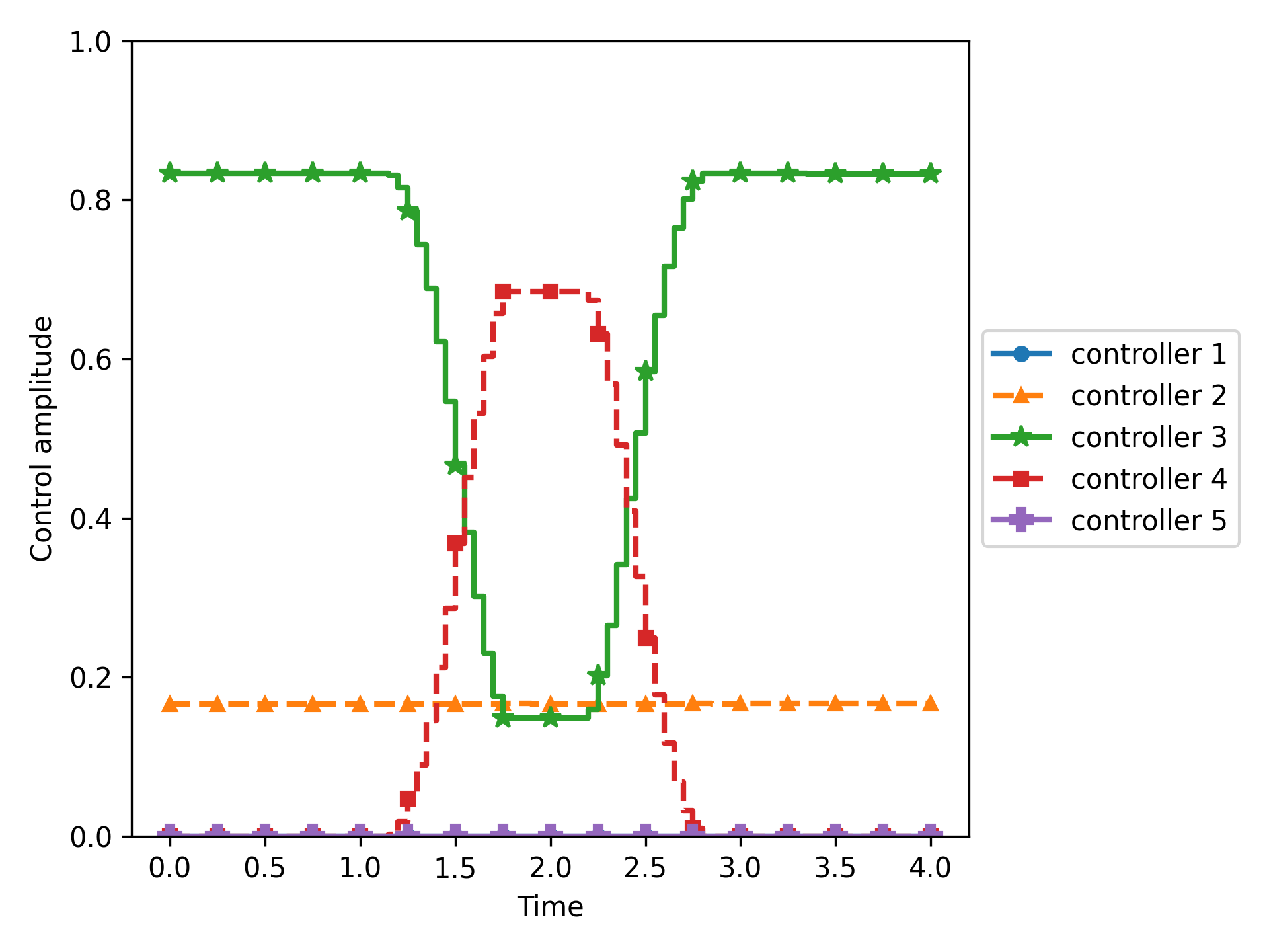
We present the continuous control results obtained from the model (DQCP-TV) in Figure 5 for the circuit compilation example on the molecule H2. We test the parameter of the TV regularizer and the Lagrangian parameter . We choose and , which has the smallest objective value after rounding with min-up-time constraints. The number of switches in control results decreases significantly as compared with the results in Figure 3, showing the benefits of the TV regularizer.
5 Improvement Heuristic: Approximate Local-Branching Method
Because the ADMM algorithm does not ensure global optimality for nonlinear objective functions and the objective value increases after rounding, the control results can be improved by applying an approximate local-branching (ALB) heuristic. The trust-region method [32] is a widely used local search method in optimization but highly depends on the initial values. In this section we propose a trust-region subproblem for the quantum control problem and then modify the trust-region method to solve the problem starting from the solutions obtained in Sections 3–4 to improve the quantum controls.
We introduce our improvement heuristic based on the approach of [69] to solve the binary model with the TV regularizer. Given a feasible point , we use the first-order gradient to approximate the objective value around the point and define the trust-region subproblem with radius as
| (29a) | ||||
| s.t. | (29b) | |||
We note that (29a) approximates the objective value but uses an exact form of the TV regularizer. Constraint (29b) indicates that we consider only the points with distance to no more than . For each controller and time step , define variables as the upper bound of the absolute change between the control values of two consecutive time steps. The trust-region subproblem is reformulated as the following mixed-integer linear program:
| (30a) | ||||
| s.t. | (30b) | |||
| (30c) | ||||
The objective function (30a) is a reformulation of (29a) with variables . Constraint (30b) is the trust-region constraint. Constraints (30c) ensure that for each controller , . Let be an optimal solution of the model (30). Define and respectively as the predictive and actual decrease of the objective function with the following formulations:
| (31a) | ||||
| (31b) | ||||
The trust-region algorithm consists of an inner loop and an outer loop. In the inner loop we solve a sequence of trust-region subproblems a with monotonically decreasing radius until the ratio between the actual decrease and predictive decrease is large enough. To obtain a balance between the computational cost and the searched area, we set a threshold for the radius. When the radius is greater than the threshold, we decrease it according to a geometric sequence [69]; otherwise, we decrease it by an arithmetic sequence. In the outer loop we repeat the inner loop for each updated point until the predictive decrease is nonpositive. This procedure is described in Algorithm 3.
Remark 7.
If we relax the feasible region of each controller to , the trust-region method can solve the continuous relaxation of the model with the TV regularizer. Trust-region methods show convergence to stationary points on continuous relaxation if we allow the radius to be real and adjusted accordingly (Corollary 3.9 in [70]).
The trust-region approach can also improve solutions obtained by CIA approaches from Section 3.3.2. Based on the restricted feasible region instead of the TV regularizer, we propose the trust-region subproblem with additional linear constraints as follows:
| (32a) | ||||
| s.t. | Constraints (3e)–(3f), (30b) | |||
| (32b) | ||||
The objective function (32a) is a first-order gradient approximation of the original objective function , and constraint (32b) restricts feasible regions for controls. The computations of the predictive decrease and actual decrease are modified as
| (33a) | ||||
| (33b) | ||||
For the trust-region algorithm (Algorithm 3), we replace solving model (30) with solving model (32) and compute the decrease by (33). The other parts remain the same.
In theory, all time-evolution processes in our algorithms can be conducted on quantum computers. The inputs for the quantum computers are the control sequences, and we require the output of the objective function and its (approximate) gradient. The updates of variables are still computed on classical computers.
6 Numerical Results
We apply our algorithmic framework proposed in Sections 3–5 to diverse instances of the four examples introduced in Section 2. In Section 6.1 we show the results from state-of-the-art optimization solvers as the baseline. In Section 6.2 we introduce the design of numerical instances and parameter settings. In Sections 6.3–6.5 we present the numerical results, including the continuous relaxation results, binary results by combinatorial integral approximation, and binary results after an improvement heuristic.
6.1 State-of-the-Art Optimization Solvers
The NEOS server is a frequently used internet-based service containing several state-of-the-art solvers for numerical optimization problems [71, 72, 73]. For nonlinear constrained continuous problems, SNOPT [74] and IPOPT [75] are two widely used solvers. For mixed-integer nonlinear constrained problems, BARON [76] and Couenne [77] are commonly used for obtaining global optimal solutions, while MINLP [78, 79], SCIP [80], and Bonmin [81] are effective solvers with good performance for finding local optima.
As a baseline we first apply the optimization solvers from the NEOS server to solve the energy minimization example problem in Section 2.1. All the experiments are conducted on the online server. We set the number of qubits and . We set the evolution time and the number of time steps . We notice that for all the evolution times in Section 6, we use dimensionless units, with . We apply the solver MUSCOD-II (6.0) [82] to solve the continuous formulation with the differential equations (1), and we set the maximum iterations to for and for . To apply the state-of-the-art nonlinear optimization solvers to a discretized model, we derive a discretized formulation of the ordinary differential equation by the implicit Euler method (see, e.g., [83]) as
| (34) |
We apply the solvers SNOPT (7.6.1) and IPOPT (3.13.4) to solve the continuous relaxation model and apply the solvers MINLP, Bonmin (1.8.8), Couenne (0.5.8), and SCIP (7.0.3.5) to solve the binary model. We set the time limit to minutes when and minutes when . In Table 2 we present the objective values, TV-norm values, CPU times, and explored nodes (only for binary solvers).
Table 2 shows that MUSCOD-II is good for solving the continuous relaxation for the instance with , but it takes a long time to solve the large instance with . SNOPT and IPOPT perform worse than the MUSCOD-II solver especially when the quantum systems include more qubits. For the binary control problem, all the methods reach the time limit. Bonmin obtains the best solution, but the gaps between their results and true energy are all large. For the instance with , some optimization solvers such as MINLP and Couenne run out of memory. The CPU time increases and the number of explored nodes decreases significantly when the size of the quantum system increases.
| Solver | ||||||
|---|---|---|---|---|---|---|
| Obj | Time (s) | Nodes | Obj | Time (s) | Nodes | |
| SNOPT | 0.084 | 0.18 | - | 0.736 | 199.64 | - |
| IPOPT | 0.084 | 0.10 | - | 0.736 | 46.85 | - |
| MUSCOD-II | E | 1.67 | - | 0.154 | 4399.54 | - |
| MINLP | 0.150 | LIMIT | 9056 | OOM | OOM | OOM |
| Bonmin | 0.148 | LIMIT | 11672 | 0.793 | LIMIT | 355 |
| Couenne | 0.471 | LIMIT | 6932 | OOM | OOM | OOM |
| SCIP | 0.149 | LIMIT | 25679 | 0.000 | LIMIT | 2480 |
This experiment shows that existing standard nonlinear programming and mixed-integer nonlinear programming solvers cannot solve discretized optimal control problems. In the following sections we present the numerical results of our proposed algorithms on multiple instances. Our pGRAPE+SUR method obtains binary solutions with an objective value E in seconds for and binary solutions with an objective value in seconds for . We show that our methods can obtain better results and with shorter computational time than do the state-of-art solvers.
6.2 Experimental Design and Parameter Settings
When the problems have no SOS1 property, the squared term in the penalized model (3.2) is eliminated, so solving (3.2) by pGRAPE is equivalent to solving the original model (3) by GRAPE. Because the energy minimization problem has only two controllers, we eliminate the SOS1 property directly by substituting . We remove the SOS1 property in the CNOT gate estimation problem to show the generality of our models. We solve the model with a squared -penalty function for the circuit compilation problem.
For all the examples, we apply the pGRAPE algorithm to solve the continuous relaxation. We also employ the TR and ADMM algorithms to solve the continuous relaxation with the TV regularizer. Then we obtain the binary results without constraints by SUR, the binary results with min-up-time constraints, and the binary results with max-switching constraints by integral minimization. Furthermore, we apply the approximate local-branching methods to improve the binary solutions with the TV regularizer and hard control constraints.
For the energy minimization problem, when , the matrix is two-dimensional and includes only one independent element because it is symmetric. Hence, we set diagonals in to and other elements to . When , we generate instances where each instance has a random symmetric matrix with zero diagonals and elements within a range . We will present averaged objective value results for these problems. The instances are represented by Energy2, Energy4, and Energy6 corresponding to the number of qubits in our following results. For the CNOT problem, we conduct experiments with evolution times and represent the corresponding instances as CNOT5, CNOT10, CNOT15, CNOT20, respectively. For the NOT gate estimation problem, we follow the parameter settings in [49] and set . We conduct numerical simulations with evolution times and represent the instances as NOT2, NOT6, and NOT10, respectively. For the circuit compilation problem, we test two molecules, H2 (dihydrogen) and LiH (lithium hydride), and generate the UCCSD circuits with minimum energy by the VQE algorithm in the Python package Qiskit [84]. The instances are represented by CircuitH2 and CircuitLiH. We set the parameters corresponding to quantum systems as . We test values of the penalty parameter for the squared -penalty function , and we choose the one with the smallest objective value among the parameters with a squared penalized term less than . We set the penalty parameter to be and for two the instances, respectively. We test values for the TV parameter and choose with the smallest rounding objective value with min-up-time constraints. The settings of and other parameters are presented in Table 3. All the numerical simulations were conducted in Python 3.8 on a MacOS computer with 8 cores, 16 GB of RAM, and a 3.20 GHz processor. All the computational time results are the times on classical computers.
| Instance | |||||||
|---|---|---|---|---|---|---|---|
| Energy2 | 2 | 2 | 2 | 40 | 0.01 | 10 | 5 |
| Energy4 | 4 | 2 | 2 | 40 | 0.01 | 10 | 5 |
| Energy6 | 6 | 2 | 2 | 40 | 0.01 | 10 | 5 |
| CNOT5 | 2 | 2 | 5 | 100 | 0.01 | 10 | 20 |
| CNOT10 | 2 | 2 | 10 | 200 | 0.001 | 10 | 20 |
| CNOT15 | 2 | 2 | 15 | 300 | 0.0001 | 10 | 20 |
| CNOT20 | 2 | 2 | 20 | 400 | 0.0001 | 10 | 20 |
| NOT2 | 1 | 2 | 2 | 20 | 0.001 | 5 | 4 |
| NOT6 | 1 | 2 | 6 | 60 | 0.001 | 5 | 12 |
| NOT10 | 1 | 2 | 10 | 100 | 0.001 | 5 | 20 |
| CircuitH2 | 2 | 5 | 4 | 80 | 0.001 | 10 | 8 |
| CircuitLiH | 4 | 12 | 20 | 200 | 0.001 | 5 | 40 |
In Sections 6.3–6.5, for brevity we select four different instances, Energy6, CNOT20, NOT10, and CircuitLiH, to analyze the results of objective values and CPU time. Detailed results of all the methods and instances are presented in Tables 4, 5, 6, 7, 8, and 9 in Appendix B. Our full code and results are available on our Github repository [85].
6.3 Results of Continuous Relaxations
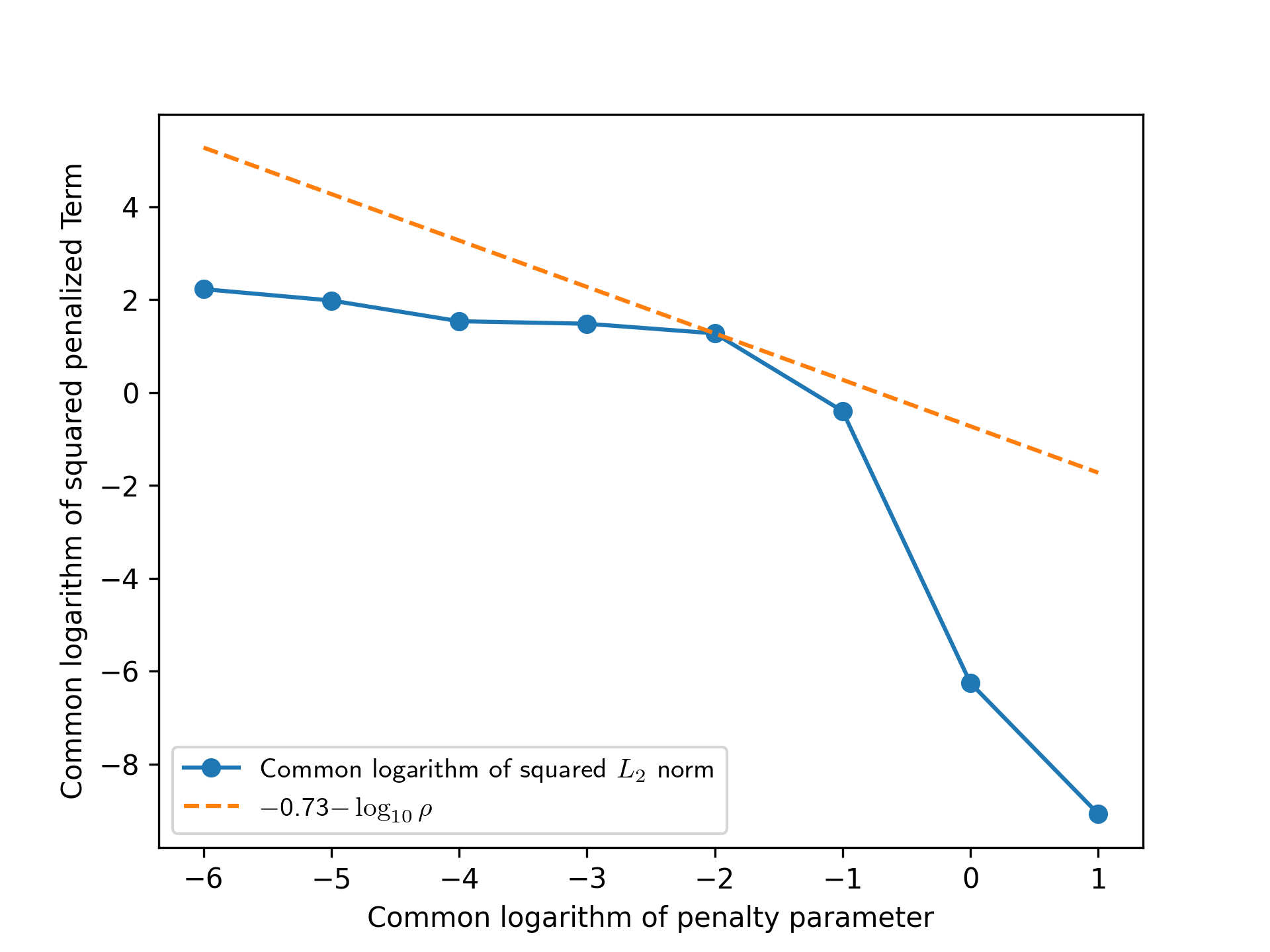
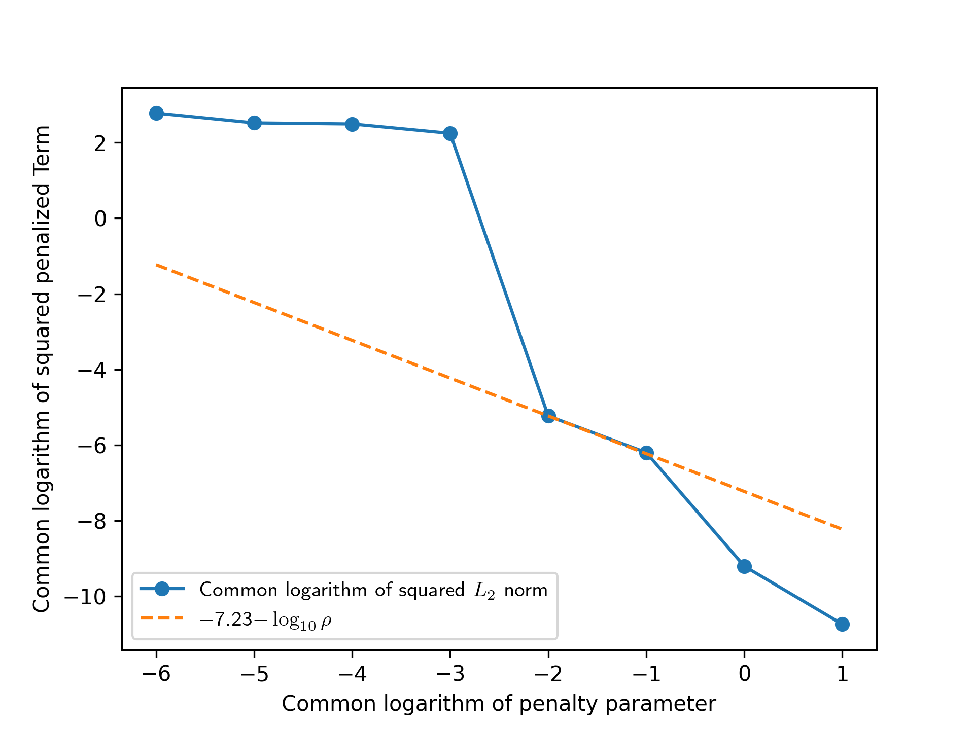
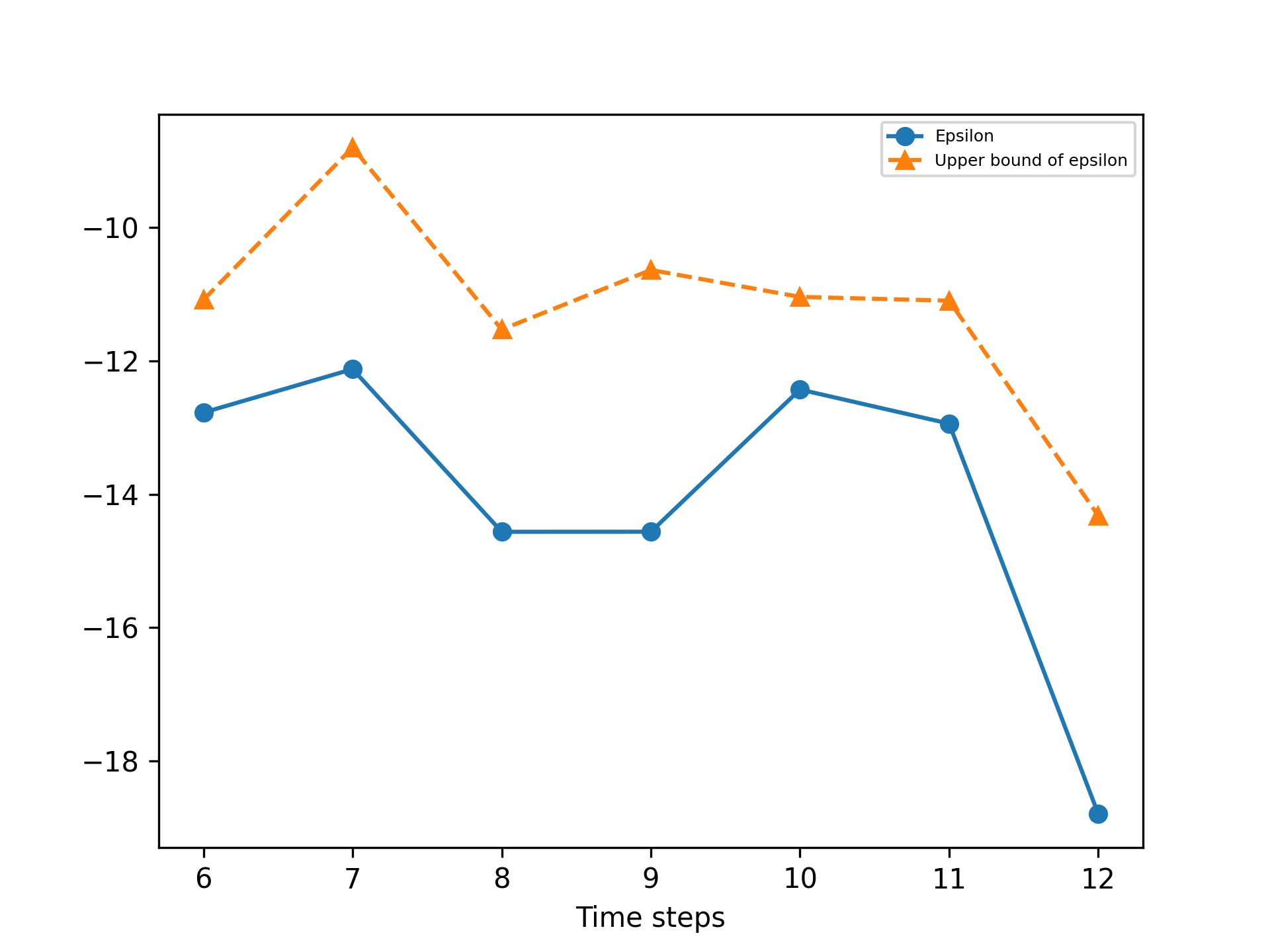
In Figure 6 we show how the common logarithm of the squared -norm value varies with the penalty parameter represented by the lines. We also present an asymptotic bound represented by the dashed lines, where is a constant marking that a selected data point lies on the dashed lines in the simulation results. Notably, the figure confirms that , as shown in Theorem 3.
We show that pGRAPE always obtains the lowest objective value but the highest TV regularizer values because it solves the model without the TV regularizer. ADMM has the best performance for reducing the TV regularizer values, showing the benefits of introducing a TV regularizer in Section 4. The detailed results are presented in Appendix B.
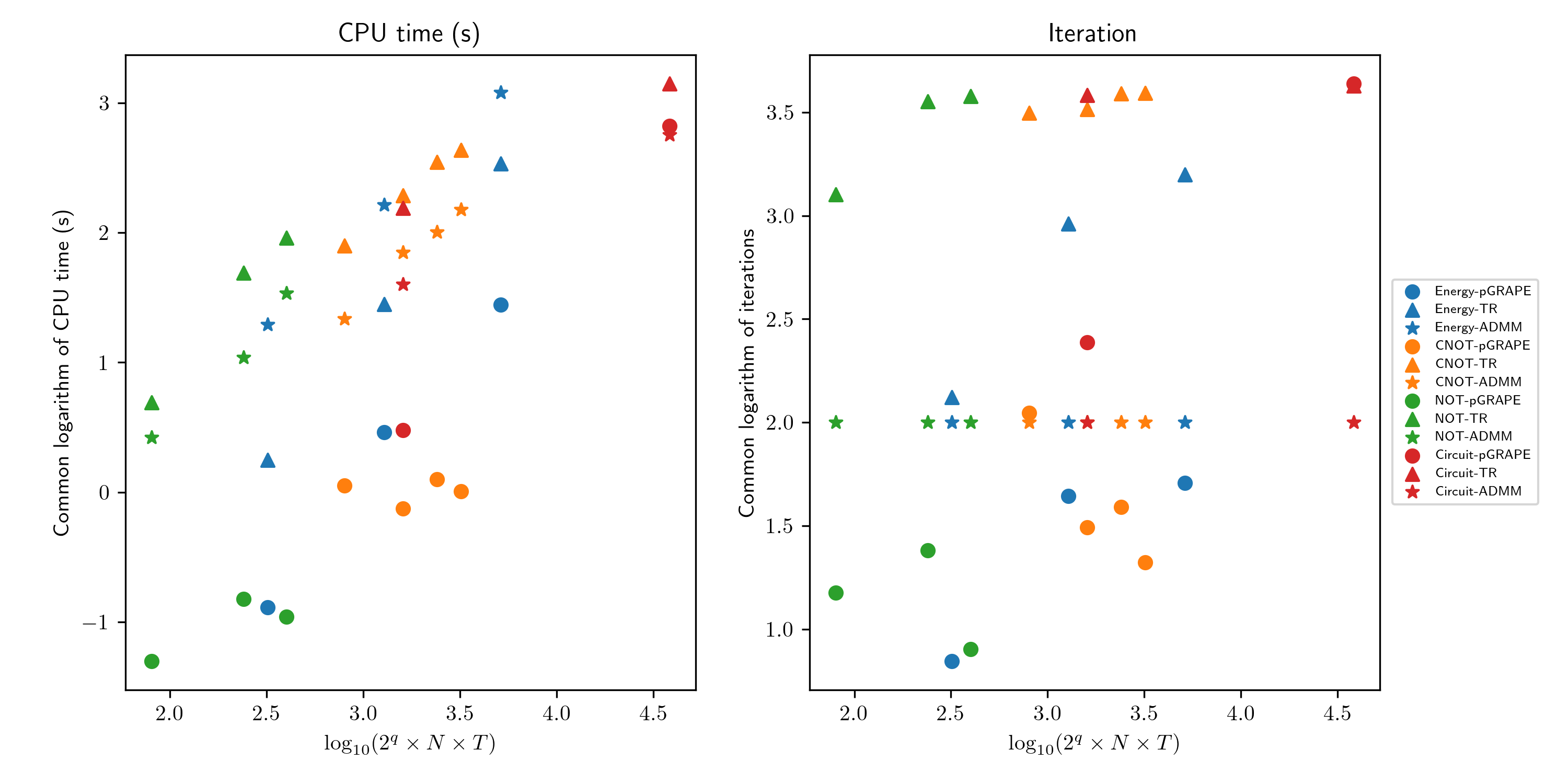
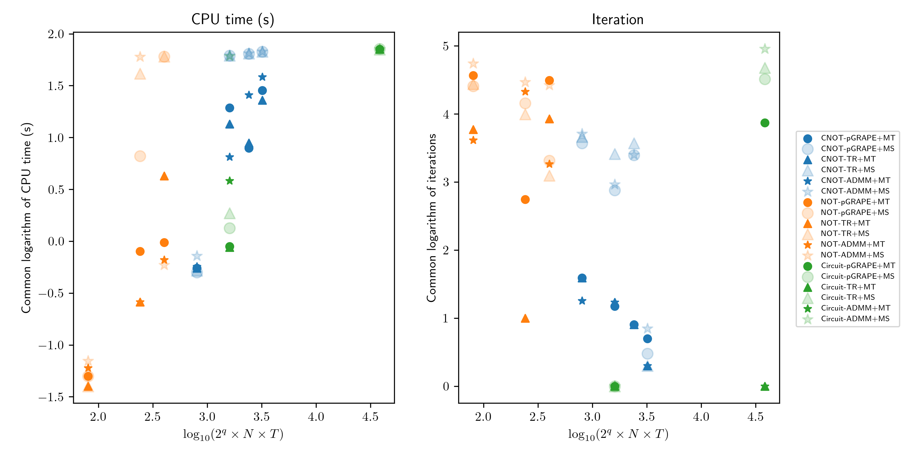
We measure the problem size of each instance by , where , , and represent the number of qubits, number of controllers, and number of time steps. For four groups of instances, Energy, CNOT, NOT, and Circuit, we present in Figure 7 common logarithm-logarithm figures to show how the CPU time and the number of iterations vary with the problem size. The CPU time increases significantly with an increase in the number of qubits because the dimension of simulation Hamiltonian matrices increases exponentially. The CPU time also increases when the number of controllers and time steps increases. Compared with pGRAPE, TR and ADMM spend more time solving the model because it contains the TV regularizer. The CPU time of ADMM is more than that of TR for Energy instances, while TR spends more time on CNOT, NOT, and Circuit instances than ADMM spends.
6.4 Results of Rounding Techniques
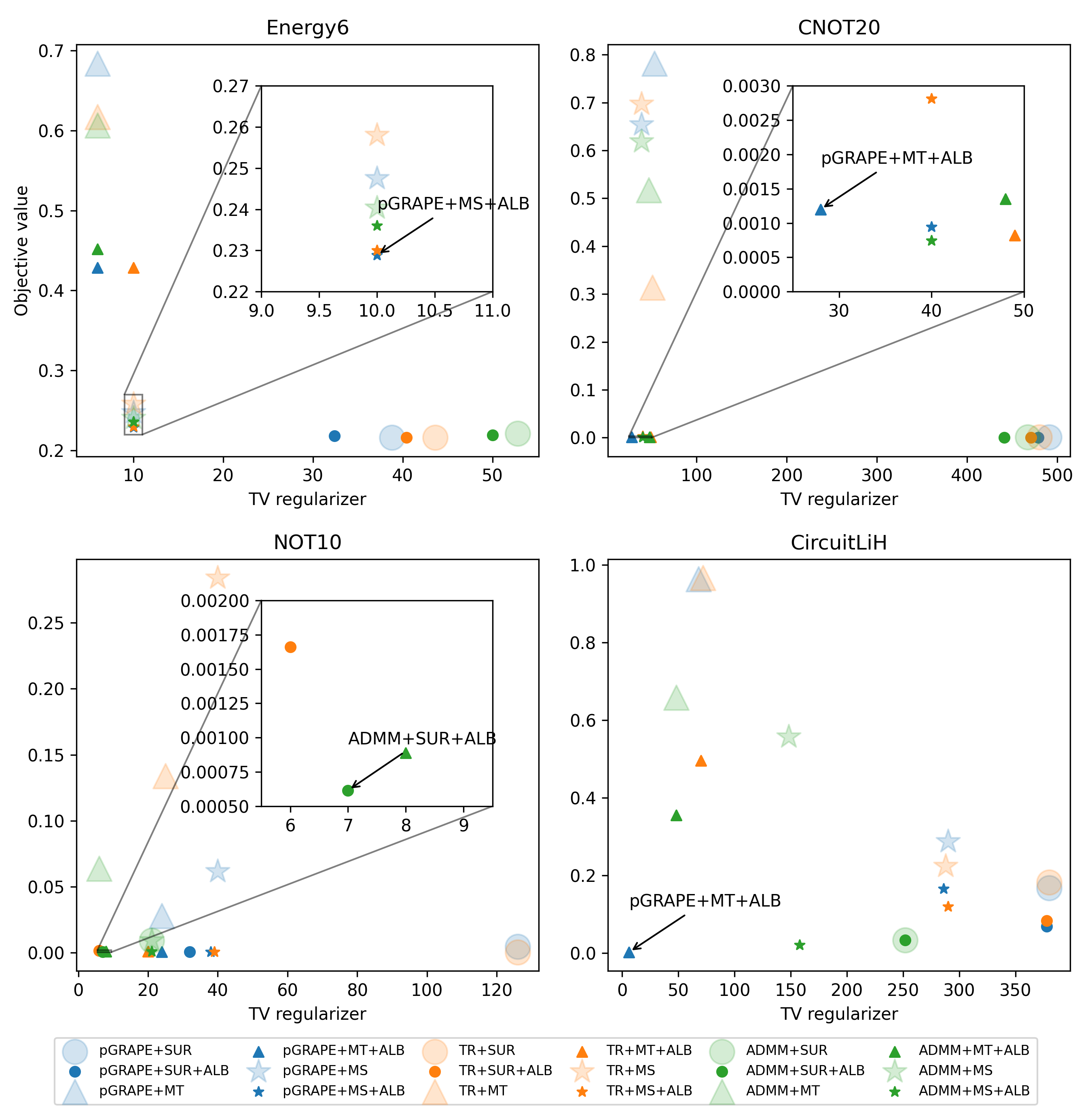
The results for Sections 6.4 and 6.5 are summarized in Figure 12, which shows the objective values and TV regularizer values of the binary results obtained by SUR as well as CIA with min-up-time constraints and max-switching constraints of selected instances. Compared with pGRAPE+MT/MS, TR+MT/MS or ADMM+MT/MS obtains lower objective values and TV regularizer values for the binary results with min-up-time constraints and max-switching constraints because they solve the model with the TV regularizer.
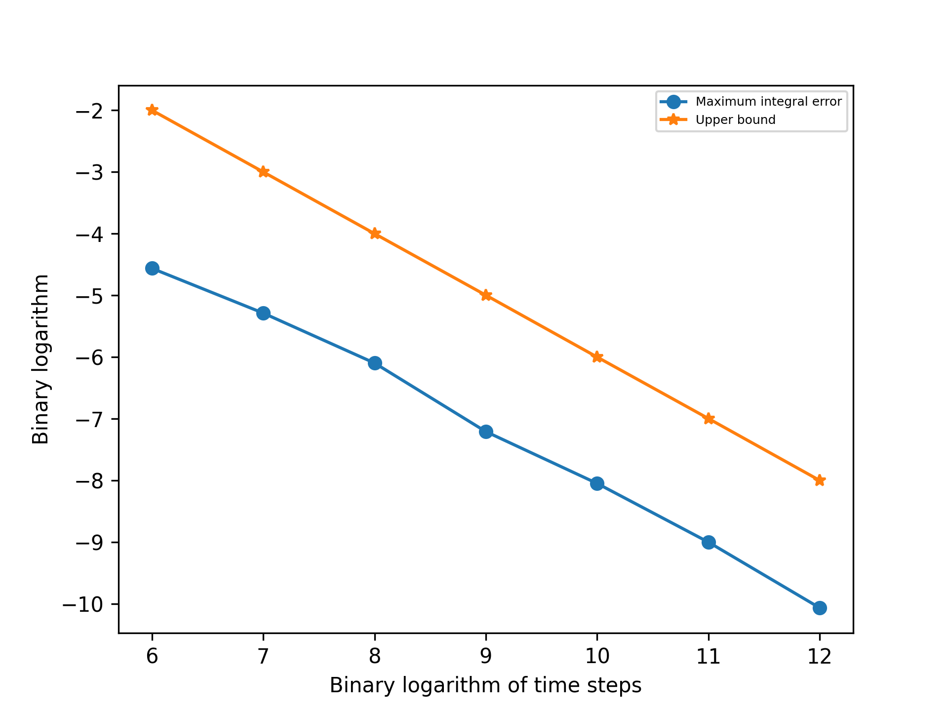
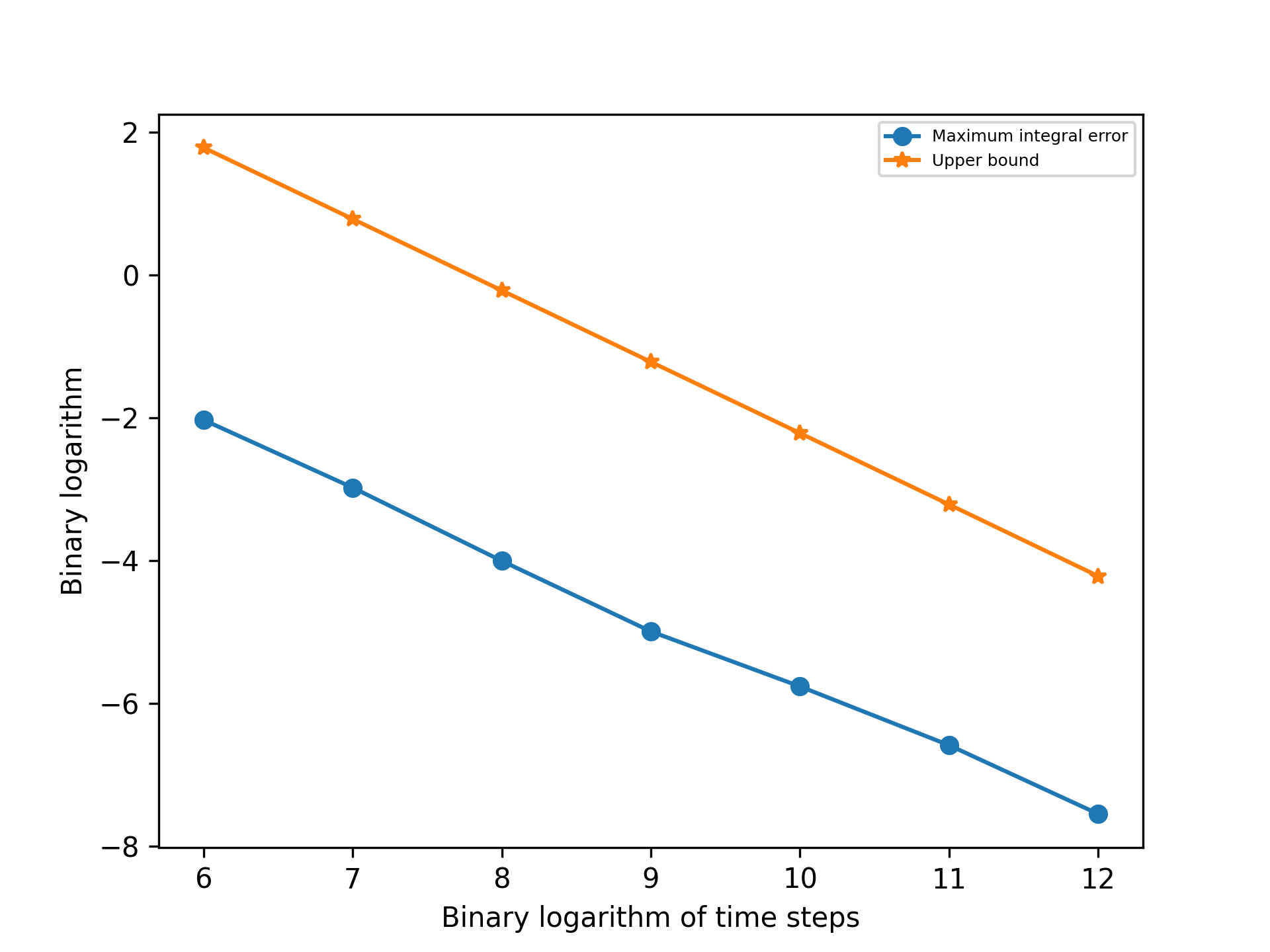
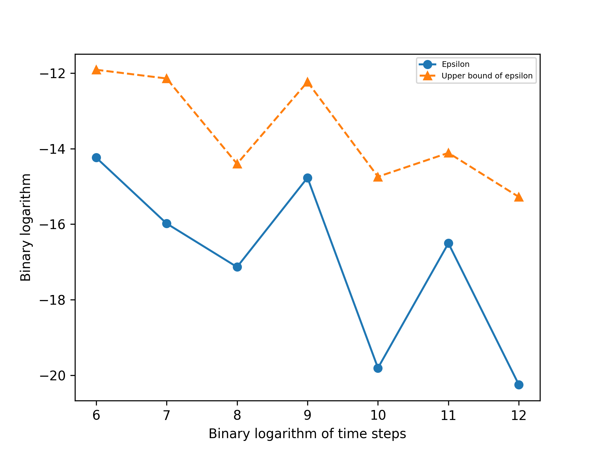
From the results of pGRAPE we show that the squared -penalty function ensures that the difference between binary controls of SUR and continuous results is small. To further demonstrate the convergence of pGRAPE+SUR in Section 3.3.1, we present how the maximum absolute integral error, which is the left-hand side of equation (21), varies with the number of time steps in Figure 8 represented by the lines. The figures show that the error converges to zero with the increase in the number of time steps, as is claimed in Proposition 2. We also present the theoretical upper bound of the integral error, which is the right-hand side of (21), represented by the dashed lines. We observe that the integral error is always less than the upper bound, demonstrating the conclusion in Theorem 4. In addition, we present the figures of how and the upper bound vary with the number of time steps for instances CircuitH2 and CircuitLiH in Figure 9. We show that is always smaller than the upper bound, demonstrating the conclusion (22) in Corollary 1.
We set the time limit to seconds for solving the combinatorial integral approximation with min-up-time and max-switching constraints. In Figure 10 we present the CPU time and iterations of all the instances. All the CPU times of SUR and Energy instances are less than 0.01 seconds so we do not show them in the figure. The CPU times increase significantly with the number of variables. For the instance CircuitLiH, all the methods exceed the computational time limit. In most cases, iterations and CPU times of MS are more than MT because the problem with MS has a larger integrality gap.
6.5 Results of Improvement Heuristic
The objective values and TV regularizer values after the improvement heuristic with the control results of combinatorial integral approximation as initial points for selected instances are represented by opaque small dots in Figure 12. Because there are multiple local minima for these quantum control problems, each method may obtain a different performance after the improvement heuristic. For systems with two controllers, all the methods obtain performance at a similar level. The performance of different methods varies more on the circuit compilation problem because it contains more local optima.
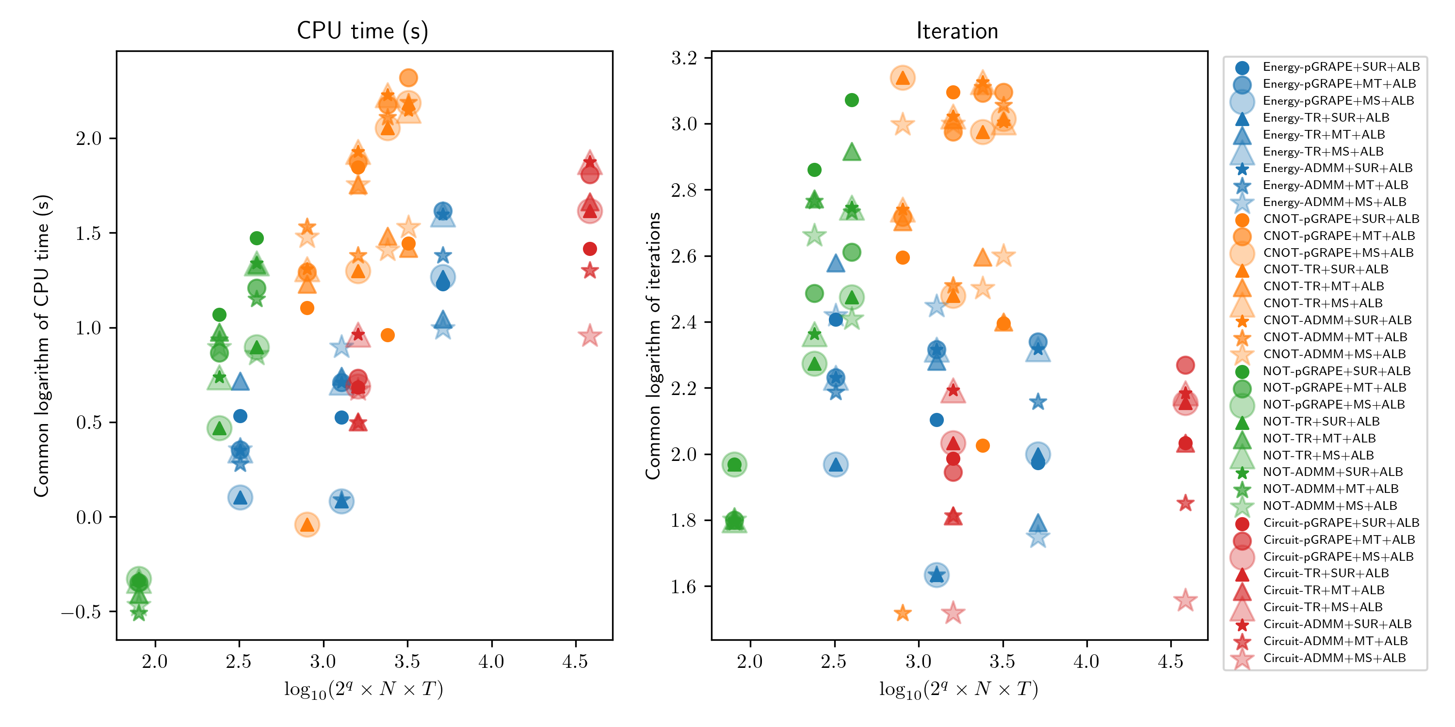
We show in Figure 11 the CPU time and iterations for the improvement heuristic of selected instances. For each group of instances Energy, CNOT, NOT, and Circuit, the CPU time increases with the problem size. The number of iterations highly depends on the initial points.
In addition, we observe that for both continuous relaxation and ALB, the CPU time is exponentially increasing but the number of iterations increases slightly. We note that the main increase of the computational time comes from the time-evolution process for simulating the quantum system because the dimension of the Hamiltonian matrices increases exponentially with the number of qubits . In our algorithm, we could directly conduct the time evolution on quantum computers with a control pulse, and then only use the final state to compute the objective value and approximate the gradient by the finite difference method. Hence, we do not need to evaluate the state at each time step, indicating the scalability of our approach for handling large-scale instances.
In Figure 12 we show the objective values and TV regularizer values of the combinatorial integral approximation and the improvement heuristic. We show that the objective value of SUR keeps the same or slightly increases, demonstrating the theorems and propositions in Section 3.3.1. Adding min-up-time and max-switching constraints leads to an increase in objective values because of adding additional constraints stated in Section 3.3.2 to the feasible set. The increase from adding min-up-time constraints is higher because the restricted feasible region contains fewer feasible solutions. From the aspect of the chattering measured by the TV regularizer value, we show that SUR leads to more chattering compared with continuous solutions because of the rounding process. As discussed in Section 3.3.2, imposing min-up-time and max-switching constraints reduces the chattering, and adding min-up-time constraints reduces it more significantly because the constraints are stricter. The improvement heuristic reduces the objective values and chattering remarkably for the results obtained from all the methods with rounding techniques, especially pGRAPE, which shows the benefits of our improvement algorithms in Section 5. In Figure 12, the dot closest to the lower-left corner indicates that it obtains the best balance between improving objective values and reducing chattering. If the original objective function matters more, one can choose methods that consist of SUR and the improvement heuristic. If one focuses more on reducing the switches, the methods with min-up-time or max-switching constraints and the improvement heuristic are better.
7 Conclusion
In this paper we built a generic control model with both continuous and discretized formulations for the quantum control problem. We introduced a penalized squared function into the model to ensure that only one control is active at all times. In addition, we proposed a model with the TV regularizer aiming to reduce the absolute change of controls.
We developed an algorithmic framework combining the GRAPE approach, combinatorial integral approximation, and local-branching improvement heuristic. With numerical simulations on multiple examples with various objective functions and controllers, we demonstrated the feasibility of the discrete optimal quantum control problem and illustrated that our algorithms obtained trade-off controls between high quality and low absolute changes within a short computational time. Specifically, the performance of different relaxation models varies among instances, and therefore, testing all three methods (pGRAPE, TR, and ADMM) is helpful to select the best control. If one is more interested in obtaining controls with a lower energy or infidelity, we recommend methods using the sum-up-rounding technique. On the other hand, if one aims to reduce switches, it is better to choose methods with min-up-time constraints added. Both cases require the use of the approximate local branching algorithm to improve final solutions. In practice, the performance can be improved further by fine-tuning the corresponding parameters.
All the numerical simulations in our paper were conducted on classical computers , and the CPU time mainly comes from the time-evolution process of quantum states. Because our algorithm only requires the final state to compute the objective value and approximate the gradient, running the time-evolution process in our algorithms on quantum computers is easy in practice and could help eliminate a significant amount of the exponential slow-down as we observe in our simulations. Furthermore, with continuous control results, we can extract appropriate controller sequences and optimize the location of switching points to obtain high-quality controls. Switching-time optimization using continuous control results is future research.
Acknowledgment
This material is based upon work supported by the U.S. Department of Energy, Office of Science, under contract number DE-AC02-06CH11357. This work was supported by the U.S. Department of Energy, Office of Science, Office of Advanced Scientific Computing Research, Accelerated Research for Quantum Computing program. The authors gratefully acknowledge the support from the Givens Associate program in Argonne National Laboratory. Xinyu Fei and Siqian Shen are thankful for the support from U.S. National Science Foundation (NSF) grants #CMMI-1727618 and Department of Energy (DOE) grant #DE-SC0018018.
Certain commercial equipment, instruments, or materials are identified in this paper in order to specify the experimental procedure adequately. Such identification is not intended to imply recommendation or endorsement by NIST, nor is it intended to imply that the materials or equipment identified are necessarily the best available for the purpose.
References
- Rabitz et al. [2000] Herschel Rabitz, Regina De Vivie-Riedle, Marcus Motzkus, and Karl Kompa. Whither the future of controlling quantum phenomena? Science, 288(5467):824–828, 2000. doi: 10.1126/science.288.5467.824.
- Werschnik and Gross [2007] J. Werschnik and E. K. U. Gross. Quantum optimal control theory. Journal of Physics B: Atomic, Molecular and Optical Physics, 40(18):R175–R211, 2007. doi: 10.1088/0953-4075/40/18/r01.
- Brif et al. [2010] Constantin Brif, Raj Chakrabarti, and Herschel Rabitz. Control of quantum phenomena: Past, present and future. New Journal of Physics, 12:075008, 2010. doi: 10.1088/1367-2630/12/7/075008.
- Shi et al. [1988] Shenghua Shi, Andrea Woody, and Herschel Rabitz. Optimal control of selective vibrational excitation in harmonic linear chain molecules. Journal of Chemical Physics, 88(11):6870–6883, 1988. doi: 10.1063/1.454384.
- Peirce et al. [1988] Anthony P. Peirce, Mohammed A. Dahleh, and Herschel Rabitz. Optimal control of quantum-mechanical systems: Existence, numerical approximation, and applications. Physical Review A, 37(12):4950–4964, 1988. doi: 10.1103/PhysRevA.37.4950.
- Shi and Rabitz [1989] Shenghua Shi and Herschel Rabitz. Selective excitation in harmonic molecular systems by optimally designed fields. Chemical Physics, 139(1):185–199, 1989. doi: 10.1016/0301-0104(89)90011-6.
- Kosloff et al. [1989] R. Kosloff, S. A. Rice, P. Gaspard, S. Tersigni, and D. J. Tannor. Wavepacket dancing: Achieving chemical selectivity by shaping light pulses. Chemical Physics, 139(1):201–220, 1989. doi: 10.1016/0301-0104(89)90012-8.
- Jakubetz et al. [1990] W. Jakubetz, J. Manz, and H. J. Schreier. Theory of optimal laser pulses for selective transitions between molecular eigenstates. Chemical Physics, 165(1):100–106, 1990. doi: 10.1016/0009-2614(90)87018-M.
- Khaneja et al. [2005] Navin Khaneja, Timo Reiss, Cindie Kehlet, Thomas Schulte-Herbrüggen, and Steffen J. Glaser. Optimal control of coupled spin dynamics: Design of NMR pulse sequences by gradient ascent algorithms. Journal of Magnetic Resonance, 172(2):296–305, 2005. doi: 10.1016/j.jmr.2004.11.004.
- Gorshkov et al. [2008] Alexey V. Gorshkov, Tommaso Calarco, Mikhail D. Lukin, and Anders S. Sørensen. Photon storage in -type optically dense atomic media, IV: Optimal control using gradient ascent. Physical Review A, 77:043806, 2008. doi: 10.1103/physreva.77.043806.
- van Bijnen and Pohl [2015] R. M. W. van Bijnen and T. Pohl. Quantum magnetism and topological ordering via Rydberg dressing near Förster resonances. Physical Review Letters, 114(24):243002, 2015. doi: 10.1103/physrevlett.114.243002.
- Palao and Kosloff [2002] José P. Palao and Ronnie Kosloff. Quantum computing by an optimal control algorithm for unitary transformations. Physical Review Letters, 89(18):188301, 2002. doi: 10.1103/PhysRevLett.89.188301.
- Palao and Kosloff [2003] José P. Palao and Ronnie Kosloff. Optimal control theory for unitary transformations. Physical Review A, 68(6):062308, 2003. doi: 10.1103/PhysRevA.68.062308.
- Montangero et al. [2007] Simone Montangero, Tommaso Calarco, and Rosario Fazio. Robust optimal quantum gates for Josephson charge qubits. Physical Review Letters, 99(17):170501, 2007. doi: 10.1103/PhysRevLett.99.170501.
- Grace et al. [2007] Matthew Grace, Constantin Brif, Herschel Rabitz, Ian A. Walmsley, Robert L. Kosut, and Daniel A. Lidar. Optimal control of quantum gates and suppression of decoherence in a system of interacting two-level particles. Journal of Physics B, 40(9):S103–S125, 2007. doi: 10.1088/0953-4075/40/9/s06.
- Waldherr et al. [2014] G. Waldherr, Y. Wang, S. Zaiser, M. Jamali, T. Schulte-Herbrüggen, H. Abe, T. Ohshima, J. Isoya, J. F. Du, P. Neumann, and J. Wrachtrup. Quantum error correction in a solid-state hybrid spin register. Nature, 506:204–207, 2014. doi: 10.1038/nature12919.
- Dolde et al. [2014] Florian Dolde, Ville Bergholm, Ya Wang, Ingmar Jakobi, Boris Naydenov, Sébastien Pezzagna, Jan Meijer, Fedor Jelezko, Philipp Neumann, Thomas Schulte-Herbrüggen, Jacob Biamonte, and Jörg Wrachtrup. High-fidelity spin entanglement using optimal control. Nature Communications, 5(3371), 2014. doi: 10.1038/ncomms4371.
- Venturelli et al. [2018] Davide Venturelli, Minh Do, Eleanor Rieffel, and Jeremy Frank. Compiling quantum circuits to realistic hardware architectures using temporal planners. Quantum Science and Technology, 3(2):025004, 2018. doi: 10.1088/2058-9565/aaa331.
- Omran et al. [2019] A. Omran, H. Levine, A. Keesling, G. Semeghini, T. T. Wang, S. Ebadi, H. Bernien, A. S. Zibrov, H. Pichler, S. Choi, J. Cui, M. Rossignolo, P. Rembold, S. Montangero, T. Calarco, M. Endres, M. Greiner, V. Vuletić, and M. D. Lukin. Generation and manipulation of Schrödinger cat states in Rydberg atom arrays. Science, 365(6453):570–574, 2019. doi: 10.1126/science.aax9743.
- Khatri et al. [2019] Sumeet Khatri, Ryan LaRose, Alexander Poremba, Lukasz Cincio, Andrew T. Sornborger, and Patrick J. Coles. Quantum-assisted quantum compiling. Quantum, 3:140, 2019. doi: 10.22331/q-2019-05-13-140.
- Yang et al. [2017] Zhi-Cheng Yang, Armin Rahmani, Alireza Shabani, Hartmut Neven, and Claudio Chamon. Optimizing variational quantum algorithms using Pontryagin’s minimum principle. Physical Review X, 7:021027, 2017. doi: 10.1103/PhysRevX.7.021027.
- Bapat and Jordan [2019] Aniruddha Bapat and Stephen Jordan. Bang-bang control as a design principle for classical and quantum optimization algorithms. Quantum Information & Computation, 19:424–446, 2019. doi: 10.26421/QIC19.5-6-4.
- Mbeng et al. [2019] Glen Bigan Mbeng, Rosario Fazio, and Giuseppe Santoro. Quantum annealing: A journey through digitalization, control, and hybrid quantum variational schemes. arXiv:1906.08948, 2019. doi: 10.48550/arXiv.1906.08948.
- Lin et al. [2019] Chungwei Lin, Yebin Wang, Grigory Kolesov, and Uroš Kalabić. Application of Pontryagin’s minimum principle to Grover’s quantum search problem. Physical Review A, 100:022327, 2019. doi: 10.1103/PhysRevA.100.022327.
- Brady et al. [2021a] Lucas T Brady, Christopher L Baldwin, Aniruddha Bapat, Yaroslav Kharkov, and Alexey V Gorshkov. Optimal protocols in quantum annealing and QAOA problems. Physical Review Letters, 126:070505, 2021a. doi: 10.1103/PhysRevLett.126.070505.
- Brady et al. [2021b] Lucas T. Brady, Lucas Kocia, Przemyslaw Bienias, Yaroslav Kharkov Aniruddha Bapat, and Alexey V. Gorshkov. Behavior of analog quantum algorithms. arXiv:2107.01218, 2021b. doi: 10.48550/arXiv.2107.01218.
- Venuti et al. [2021] Lorenzo Campos Venuti, Domenico D’Alessandro, and Daniel A. Lidar. Optimal control for quantum optimization of closed and open systems. Physical Review Applied, 16(5), 2021. doi: 10.1103/physrevapplied.16.054023.
- Kadowaki and Nishimori [1998] Tadashi Kadowaki and Hidetoshi Nishimori. Quantum annealing in the transverse Ising model. Physical Review E, 58:5355, 1998. doi: 10.1103/PhysRevE.58.5355.
- Farhi et al. [2000] Edward Farhi, Jeffrey Goldstone, Sam Gutmann, and Michael Sipser. Quantum computation by adiabatic evolution. arXiv:quant-ph/0001106, 2000. doi: 10.48550/arXiv.quant-ph/0001106.
- Pagano et al. [2020] Guido Pagano, Aniruddha Bapat, Patrick Becker, Katherine S. Collins, Arinjoy De, Paul W. Hess, Harvey B. Kaplan, Antonis Kyprianidis, Wen Lin Tan, Christopher Baldwin, Lucas T. Brady, Abhinav Deshpande, Fangli Liu, Stephen Jordan, Alexey V. Gorshkov, and Christopher Monroe. Quantum approximate optimization of the long-range Ising model with a trapped-ion quantum simulator. PNAS, 117(41):25396–25401, 2020. doi: 10.1073/pnas.2006373117.
- Harrigan et al. [2021] Matthew P. Harrigan, Kevin J. Sung, Matthew Neeley, Kevin J. Satzinger, Frank Arute, Kunal Arya, Juan Atalaya, Joseph C. Bardin, Rami Barends, Sergio Boixo, Michael Broughton, Bob B. Buckley, David A. Buell, Brian Burkett, Nicholas Bushnell, Yu Chen, Zijun Chen, Ben Chiaro, Roberto Collins, William Courtney, Sean Demura, Andrew Dunsworth, Daniel Eppens, Austin Fowler, Brooks Foxen, Craig Gidney, Marissa Giustina, Rob Graff, Steve Habegger, Alan Ho, Sabrina Hong, Trent Huang, L. B. Ioffe, Sergei V. Isakov, Evan Jeffrey, Zhang Jiang, Cody Jones, Dvir Kafri, Kostyantyn Kechedzhi, Julian Kelly, Seon Kim, Paul V. Klimov, Alexander N. Korotkov, Fedor Kostritsa, David Landhuis, Pavel Laptev, Mike Lindmark, Martin Leib, Orion Martin, John M. Martinis, Jarrod R. McClean, Matt McEwen, Anthony Megrant, Xiao Mi, Masoud Mohseni, Wojciech Mruczkiewicz, Josh Mutus, Ofer Naaman, Charles Neill, Florian Neukart, Murphy Yuezhen Niu, Thomas E. O’Brien, Bryan O’Gorman, Eric Ostby, Andre Petukhov, Harald Putterman, Chris Quintana, Pedram Roushan, Nicholas C. Rubin, Daniel Sank, Andrea Skolik, Vadim Smelyanskiy, Doug Strain, Michael Streif, Marco Szalay, Amit Vainsencher, Theodore White, Z. Jamie Yao, Ping Yeh, Adam Zalcman, Leo Zhou, Hartmut Neven, Dave Bacon, Erik Lucero, Edward Farhi, and Ryan Babbush. Quantum approximate optimization of non-planar graph problems on a planar superconducting processor. Nature Physics, 17:332–336, 2021. doi: 10.1038/s41567-020-01105-y.
- Nocedal and Wright [2006] Jorge Nocedal and Stephen Wright. Numerical Optimization. Springer Science & Business Media, 2006. doi: 10.1007/978-0-387-40065-5.
- Larocca and Wisniacki [2021] Martín Larocca and Diego Wisniacki. Krylov-subspace approach for the efficient control of quantum many-body dynamics. Physical Review A, 103(2), 2021. doi: 10.1103/physreva.103.023107.
- Doria et al. [2011] Patrick Doria, Tommaso Calarco, and Simone Montangero. Optimal control technique for many-body quantum dynamics. Physical Review Letters, 106(19):190501, 2011. doi: 10.1103/PhysRevLett.106.190501.
- Caneva et al. [2011] Tommaso Caneva, Tommaso Calarco, and Simone Montangero. Chopped random-basis quantum optimization. Physical Review A, 84(2):022326, 2011. doi: 10.1103/physreva.84.022326.
- Sørensen et al. [2018] J. J. W. H. Sørensen, M. O. Aranburu, T. Heinzel, and J. F. Sherson. Quantum optimal control in a chopped basis: Applications in control of Bose-Einstein condensates. Physical Review A, 98(2):022119, 2018. doi: 10.1103/PhysRevA.98.022119.
- Farhi et al. [2014] Edward Farhi, Jeffrey Goldstone, and Sam Gutmann. A quantum approximate optimization algorithm. arXiv:1411.4028, 2014. doi: 10.48550/arXiv.1411.4028.
- Bharti et al. [2022] Kishor Bharti, Alba Cervera-Lierta, Thi Ha Kyaw, Tobias Haug, Sumner Alperin-Lea, Abhinav Anand, Matthias Degroote, Hermanni Heimonen, Jakob S. Kottmann, Tim Menke, Wai-Keong Mok, Sukin Sim, Leong-Chuan Kwek, and Alán Aspuru-Guzik. Noisy intermediate-scale quantum algorithms. Reviews of Modern Physics, 94(1), 2022. doi: 10.1103/revmodphys.94.015004.
- Cerezo et al. [2021] M. Cerezo, Andrew Arrasmith, Ryan Babbush, Simon C. Benjamin, Suguru Endo, Keisuke Fujii, Jarrod R. McClean, Kosuke Mitarai, Xiao Yuan, Lukasz Cincio, and Patrick J. Coles. Variational quantum algorithms. Nature Reviews Physics, 3(9):625–644, 2021. doi: 10.1038/s42254-021-00348-9.
- Liang et al. [2020] Daniel Liang, Li Li, and Stefan Leichenauer. Investigating quantum approximate optimization algorithms under bang-bang protocols. Physical Review Research, 2(3):033402, 2020. doi: 10.1103/physrevresearch.2.033402.
- Bao et al. [2018] Seraph Bao, Silken Kleer, Ruoyu Wang, and Armin Rahmani. Optimal control of superconducting gmon qubits using Pontryagin’s minimum principle: Preparing a maximally entangled state with singular bang-bang protocols. Physical Review A, 97(6):062343, 2018. doi: 10.1103/physreva.97.062343.
- Mühlenbein et al. [1988] Heinz Mühlenbein, Martina Gorges-Schleuter, and Ottmar Krämer. Evolution algorithms in combinatorial optimization. Parallel Computing, 7(1):65–85, 1988. doi: 10.1016/0167-8191(88)90098-1.
- Lawler and Wood [1966] Eugene L Lawler and David E Wood. Branch-and-bound methods: A survey. Operations Research, 14(4):699–719, 1966. doi: 10.1287/opre.14.4.699.
- Leyffer [2001] Sven Leyffer. Integrating SQP and branch-and-bound for mixed integer nonlinear programming. Computational Optimization and Applications, 18(3):295–309, 2001. doi: 10.1023/A:1011241421041.
- Vogt and Petersson [2022] Ryan H. Vogt and N. Anders Petersson. Binary optimal control of single-flux-quantum pulse sequences. SIAM Journal on Control and Optimization, 60(6):3217–3236, 2022. doi: 10.1137/21m142808x.
- Zahedinejad et al. [2014] Ehsan Zahedinejad, Sophie Schirmer, and Barry C Sanders. Evolutionary algorithms for hard quantum control. Physical Review A, 90(3):032310, 2014. doi: 10.1103/PhysRevA.90.032310.
- Sager et al. [2012] Sebastian Sager, Hans Georg Bock, and Moritz Diehl. The integer approximation error in mixed-integer optimal control. Mathematical Programming, 133(1):1–23, 2012. doi: 10.1007/s10107-010-0405-3.
- Pawela and Sadowski [2016] Łukasz Pawela and Przemysław Sadowski. Various methods of optimizing control pulses for quantum systems with decoherence. Quantum Information Processing, 15(5):1937–1953, 2016. doi: 10.1007/s11128-016-1242-y.
- Motzoi et al. [2009] F. Motzoi, J. M. Gambetta, P. Rebentrost, and F. K. Wilhelm. Simple pulses for elimination of leakage in weakly nonlinear qubits. Physical Review Letters, 103(11), 2009. doi: 10.1103/physrevlett.103.110501.
- Bartlett and Musiał [2007] Rodney J. Bartlett and Monika Musiał. Coupled-cluster theory in quantum chemistry. Reviews of Modern Physics, 79(1):291, 2007. doi: 10.1103/RevModPhys.79.291.
- Romero et al. [2018] Jonathan Romero, Ryan Babbush, Jarrod R McClean, Cornelius Hempel, Peter J. Love, and Alán Aspuru-Guzik. Strategies for quantum computing molecular energies using the unitary coupled cluster ansatz. Quantum Science and Technology, 4(1):014008, 2018. doi: 10.1088/2058-9565/aad3e4.
- Chen et al. [2014] Yu Chen, C Neill, P Roushan, N Leung, M Fang, R Barends, J Kelly, B Campbell, Z Chen, B Chiaro, et al. Qubit architecture with high coherence and fast tunable coupling. Physical Review Letters, 113(22):220502, 2014. doi: 10.1103/PhysRevLett.113.220502.
- Gokhale et al. [2019] Pranav Gokhale, Yongshan Ding, Thomas Propson, Christopher Winkler, Nelson Leung, Yunong Shi, David I. Schuster, Henry Hoffmann, and Frederic T Chong. Partial compilation of variational algorithms for noisy intermediate-scale quantum machines. In Proceedings of the 52nd Annual IEEE/ACM International Symposium on Microarchitecture, pages 266–278, 2019. doi: 10.1145/3352460.3358313.
- Jurdjevic and Sussmann [1972] Velimir Jurdjevic and Héctor J Sussmann. Control systems on Lie groups. Journal of Differential Equations, 12(2):313–329, 1972. doi: 10.1016/0022-0396(72)90035-6.
- Ramakrishna et al. [1995] Viswanath Ramakrishna, Murti V. Salapaka, Mohammed Dahleh, Herschel Rabitz, and Anthony Peirce. Controllability of molecular systems. Physical Review A, 51(2):960, 1995. doi: 10.1103/PhysRevA.51.960.
- Byrd et al. [1995] Richard H Byrd, Peihuang Lu, Jorge Nocedal, and Ciyou Zhu. A limited memory algorithm for bound constrained optimization. SIAM Journal on Scientific Computing, 16(5):1190–1208, 1995. doi: 10.1137/0916069.
- Sinclair [1986] Marius Sinclair. An exact penalty function approach for nonlinear integer programming problems. European Journal of Operational Research, 27(1):50–56, 1986. doi: 10.1016/S0377-2217(86)80006-6.
- You and Leyffer [2011] Fengqi You and Sven Leyffer. Mixed-integer dynamic optimization for oil-spill response planning with integration of a dynamic oil weathering model. AIChE Journal, 57(12):3555–3564, 2011. doi: 10.1002/aic.12536.
- Manns and Kirches [2020] Paul Manns and Christian Kirches. Multidimensional sum-up rounding for elliptic control systems. SIAM Journal on Numerical Analysis, 58(6):3427–3447, 2020. doi: 10.1137/19M1260682.
- Sager [2005] Sebastian Sager. Numerical Methods for Mixed-Integer Optimal Control Problems. PhD thesis, 2005.
- Wolsey [2020] Laurence A Wolsey. Integer Programming. John Wiley & Sons, 2020. doi: 10.1002/9781119606475.
- Rudin et al. [1992] Leonid I Rudin, Stanley Osher, and Emad Fatemi. Nonlinear total variation based noise removal algorithms. Physica D: Nonlinear Phenomena, 60(1-4):259–268, 1992. doi: 10.1016/0167-2789(92)90242-F.
- Condat [2013] Laurent Condat. A direct algorithm for 1-D total variation denoising. IEEE Signal Processing Letters, 20(11):1054–1057, 2013. doi: 10.1109/LSP.2013.2278339.
- Kunisch and Hintermüller [2004] Karl Kunisch and Michael Hintermüller. Total bounded variation regularization as a bilaterally constrained optimization problem. SIAM Journal on Applied Mathematics, 64(4):1311–1333, 2004. doi: 10.1137/S0036139903422784.
- Rodríguez [2013] Paul Rodríguez. Total variation regularization algorithms for images corrupted with different noise models: A review. Journal of Electrical and Computer Engineering, 2013, 2013. doi: 10.1155/2013/217021.
- Stella et al. [2017] Lorenzo Stella, Andreas Themelis, Pantelis Sopasakis, and Panagiotis Patrinos. A simple and efficient algorithm for nonlinear model predictive control. In 56th Annual Conference on Decision and Control, pages 1939–1944. IEEE, 2017. doi: 10.1109/CDC.2017.8263933.
- Themelis et al. [2018] Andreas Themelis, Lorenzo Stella, and Panagiotis Patrinos. Forward-backward envelope for the sum of two nonconvex functions: Further properties and nonmonotone linesearch algorithms. SIAM Journal on Optimization, 28(3):2274–2303, 2018. doi: 10.1137/16M1080240.
- Sager and Zeile [2021] Sebastian Sager and Clemens Zeile. On mixed-integer optimal control with constrained total variation of the integer control. Computational Optimization and Applications, 78(2):575–623, 2021. doi: 10.1007/s10589-020-00244-5.
- Leyffer and Manns [2021] Sven Leyffer and Paul Manns. Sequential linear integer programming for integer optimal control with total variation regularization. arXiv:2106.13453, 2021. doi: 10.48550/arXiv.2106.13453.
- Aravkin et al. [2022] Aleksandr Y. Aravkin, Robert Baraldi, and Dominique Orban. A proximal quasi-Newton trust-region method for nonsmooth regularized optimization. SIAM Journal on Optimization, 32(2):900–929, 2022. doi: 10.1137/21m1409536.
- Czyzyk et al. [1998] Joseph Czyzyk, Michael P. Mesnier, and Jorge J. Moré. The NEOS server. IEEE Journal on Computational Science and Engineering, 5(3):68–75, 1998. doi: 10.1109/99.714603.
- Dolan [2001] Elizabeth D. Dolan. The NEOS server 4.0 administrative guide. Technical Memorandum ANL/MCS-TM-250, Mathematics and Computer Science Division, Argonne National Laboratory, 2001.
- Gropp and Moré [1997] William Gropp and Jorge J. Moré. Optimization environments and the NEOS server. In Martin D. Buhman and Arieh Iserles, editors, Approximation Theory and Optimization, pages 167–182. Cambridge University Press, 1997.
- Andrei [2017] Neculai Andrei. A SQP algorithm for large-scale constrained optimization: SNOPT. In Continuous nonlinear optimization for engineering applications in GAMS technology, pages 317–330. Springer, 2017. doi: 10.1007/978-3-319-58356-3.
- Wächter and Biegler [2006] Andreas Wächter and Lorenz T Biegler. On the implementation of an interior-point filter line-search algorithm for large-scale nonlinear programming. Mathematical Programming, 106(1):25–57, 2006. doi: 10.1007/s10107-004-0559-y.
- Sahinidis [1996] Nikolaos V Sahinidis. BARON: A general purpose global optimization software package. Journal of Global Optimization, 8(2):201–205, 1996. doi: 10.1007/bf00138693.
- Belotti [2009] Pietro Belotti. Couenne: A user’s manual. Technical report, Lehigh University, 2009.
- Belotti et al. [2013] Pietro Belotti, Christian Kirches, Sven Leyffer, Jeff Linderoth, James Luedtke, and Ashutosh Mahajan. Mixed-integer nonlinear optimization. Acta Numerica, 22:1–131, 2013. doi: 10.1017/S0962492913000032.
- Leyffer and Mahajan [2011] Sven Leyffer and Ashutosh Mahajan. Software for nonlinearly constrained optimization. In James J. Cochran, Louis A. Cox, Pinar Keskinocak, Jeffrey P. Kharoufeh, and J. Cole Smith, editors, Wiley Encyclopedia of Operations Research and Management Science. John Wiley & Sons, Inc., 2011. doi: 10.1002/9780470400531.eorms0570.
- Gamrath et al. [2020] Gerald Gamrath, Daniel Anderson, Ksenia Bestuzheva, Wei-Kun Chen, Leon Eifler, Maxime Gasse, Patrick Gemander, Ambros Gleixner, Leona Gottwald, Katrin Halbig, Gregor Hendel, Christopher Hojny, Thorsten Koch, Pierre Le Bodic, Stephen J. Maher, Frederic Matter, Matthias Miltenberger, Erik Mühmer, Benjamin Müller, Marc E. Pfetsch, Franziska Schlösser, Felipe Serrano, Yuji Shinano, Christine Tawfik, Stefan Vigerske, Fabian Wegscheider, Dieter Weninger, and Jakob Witzig. The SCIP Optimization Suite 7.0. ZIB-Report 20-10, Zuse Institute Berlin, 2020.
- Bonami et al. [2008] Pierre Bonami, Lorenz T. Biegler, Andrew R. Conn, Gérard Cornuéjols, Ignacio E. Grossmann, Carl D. Laird, Jon Lee, Andrea Lodi, François Margot, Nicolas Sawaya, and Andreas Wächter. An algorithmic framework for convex mixed integer nonlinear programs. Discrete optimization, 5(2):186–204, 2008. doi: 10.1016/j.disopt.2006.10.011.
- Kirches and Leyffer [2013] Christian Kirches and Sven Leyffer. TACO: A toolkit for AMPL control optimization. Mathematical Programming Computation, 5(3):227–265, 2013. doi: 10.1007/s12532-013-0054-7.
- Butcher [2016] John Charles Butcher. Numerical Methods for Ordinary Differential Equations. John Wiley & Sons, 2016. doi: 10.1002/9781119121534.
- Aleksandrowicz et al. [2021] Gadi Aleksandrowicz, Thomas Alexander, Panagiotis Barkoutsos, Luciano Bello, Yael Ben-Haim, David Bucher, Francisco Jose Cabrera-Hernández, Jorge Carballo-Franquis, Adrian Chen, Chun-Fu Chen, et al. Qiskit: An open-source framework for quantum computing. 2021. doi: 10.5281/ZENODO.2562110.
- Fei [2022] Xinyu Fei. Code and Results: Binary Control Pulse Optimization for Quantum Systems. https://github.com/xinyufei/Quantum-Control-qutip, 2022.
- Rebentrost and Wilhelm [2009] Patrick Rebentrost and Frank K Wilhelm. Optimal control of a leaking qubit. Physical Review B, 79(6):060507, 2009. doi: 10.1103/physrevb.79.060507.
Appendix A Proofs of Results in Section 3
In this section, we provide proofs of the results in Section 3.
A.1 Proofs of Results in Section 3.2
Proof of Theorem 3.
Because is upper bounded by constant , we have for all the . We prove that for any and , . Assume that there exists an optimal solution of (3.2) such that , then we have . This is a contradiction to the definition of because we can find a feasible solution of (3) such that . Therefore we drive that , which means that . ∎
A.2 Proofs of Results in Section 3.3
Proof of Proposition 1.
Because the SOS1 property holds for binary control , we have
| (35) |
∎
Proof of Theorem 4.
For simplicity, we use to denote . It is obvious that for any time step , exactly one control can be set to by by the construction. Hence satisfies the SOS1 property. For a specific time step , define
| (36) |
We assume that there exists a time step such that the claim does not hold. For simplicity, we use to represent the corresponding . We consider the assumption in two cases.
Case 1:
We assume that,
| (37) |
Let be the highest index of the time step in which control is rounded up,
| (38) |
Then by (37), we have,
| (39a) | ||||
| (39b) | ||||
Because , we know that has the maximum value of (39a) among . Hence it follows from (39),
| (40) |
Summing up over all the controls ,
| (41) |
The first inequality comes from the definition of . This leads to , which is a contradiction because and .
Case 2:
We assume that,
| (42) |
From the definition of , we have
| (43) |
and by substituting (42) into (43), it holds that
| (44) |
Because the left-hand side can be written as the sum of terms as
| (45) |
at least one of them must be negative, therefore there exists such that
| (46) |
Let be the highest index of the time step in which control is rounded up,
| (47) |
Then we have
| (48) |
The first inequality follows from and . The second inequality follows from (46). Because is the control which is rounded up at time step , for any , it holds that,
| (49) |
Summing over all the controls, we have
| (50) |
This contradicts the definition of the parameter . ∎
Proof of Corollary 1.
Based on the formulation of the discretized control in the continuous relaxation of the model (3.2), we have
| (51) |
From Theorem 4, we directly obtain the statement (22). From Theorem 3, if the original function is bounded, the optimized squared term is uniformly bounded over time steps , then the absolute integral error between continuous and discretized control converges with . ∎
Proof of Proposition 2.
For any time step , we have
| (52) |
The last equality follows by Trotter expansion that and taking the limit as goes to zero. Similarly, for binary control, we have
| (53) |
From Theorem 4, we have for any time step and controller ,
| (54) |
Combining with Corollary 1 and taking the limit as goes to zero, we have
| (55) |
We substitute (55) into the formulation of states (A.2) and (53), then we obtain the conclusion that
| (56) |
Substituting states into the objective function, we prove that
| (57) |
∎
Appendix B Detailed Numerical Results
In this section, we present the results of continuous relaxation, combinatorial integral approximation, and the improvement heuristic for all the methods and instances in Table 4–9. We also present the objective values and TV regularizer values for all the instances and annotate the best method in Figure 13.
| Instance | Objective value | TV regularizer | ||||
|---|---|---|---|---|---|---|
| pGRAPE | TR | ADMM | pGRAPE | TR | ADMM | |
| Energy2 | 1.10E | 9.11E | 8.94E | 0.999 | 0.567 | 0.523 |
| Energy4 | 0.154 | 0.155 | 0.168 | 5.064 | 4.114 | 2.752 |
| Energy6 | 5.999 | 4.508 | 3.237 | |||
| CNOT5 | 0.169 | 0.124 | 0.191 | 16.000 | 9.419 | 6.094 |
| CNOT10 | 1.16E | 2.65E | 3.21E | 20.979 | 15.194 | 11.056 |
| CNOT15 | 1.00E | 8.43E | 3.65E | 29.846 | 24.348 | 16.795 |
| CNOT20 | 5.93E | 4.06E | 8.07E | 26.162 | 23.481 | 15.099 |
| NOT2 | 0.163 | 0.163 | 0.163 | 2.226 | 1.188 | 0.908 |
| NOT6 | 4.28E10 | 6.55E05 | 1.07E04 | 3.251 | 0.652 | 0.578 |
| NOT10 | 6.55E11 | 5.14E05 | 4.79E05 | 2.740 | 1.530 | 1.005 |
| CircuitH2 | 4.37E | 1.24E | 1.33E | 18.720 | 8.421 | 2.744 |
| CircuitLiH | 1.14E | 1.45E | 1.43E | 53.976 | 48.720 | 0.677 |
| Instance | CPU time (s) | Iterations | ||||
|---|---|---|---|---|---|---|
| pGRAPE | TR | ADMM | pGRAPE | TR | ADMM | |
| Energy2 | 0.13 | 1.77 | 19.56 | 7 | 132 | 100 |
| Energy4 | 2.89 | 27.99 | 163.08 | 44 | 914 | 100 |
| Energy6 | 27.94 | 341.43 | 1195.41 | 51 | 1578 | 100 |
| CNOT5 | 1.12 | 79.55 | 21.75 | 111 | 3146 | 100 |
| CNOT10 | 0.75 | 192.78 | 70.21 | 31 | 3279 | 100 |
| CNOT15 | 1.26 | 348.96 | 100.59 | 39 | 3900 | 100 |
| CNOT20 | 1.02 | 432.73 | 150.25 | 21 | 3929 | 100 |
| NOT2 | 0.05 | 4.93 | 2.63 | 15 | 1268 | 100 |
| NOT6 | 0.15 | 48.81 | 10.93 | 24 | 3563 | 100 |
| NOT10 | 0.10 | 91.39 | 34.05 | 6 | 3762 | 100 |
| CircuitH2 | 3.01 | 154.05 | 39.86 | 244 | 3832 | 100 |
| CircuitLiH | 663.08 | 1403.03 | 564.95 | 4345 | 4247 | 100 |
Instance Objective value/TV regularizer pGRAPE+SUR TR+SUR ADMM+SUR pGRAPE+MT TR+MT ADMM+MT pGRAPE+MS TR+MS ADMM+MS Energy2 4.22E/54 4.91E/54 4.01E/48 /4 /6 /6 /10 /10 /10 Energy4 /26.8 /32.4 /44.8 /6 /6 /6 /10 /10 /10 Energy6 /38.8 /43.6 /52.8 /6 /6 /6 /10 /10 /10 CNOT5 0.170/16 0.332/24 0.190/41 0.243/10 0.525/6 0.285/7 0.170/16 0.593/15 0.191/32 CNOT10 6.01E/116 1.78E/116 1.68E/86 0.158/22 0.323/21 0.084/15 0.011/39 0.019/38 0.006/32 CNOT15 1.12E/266 2.30E/276 2.90E/279 0.539/37 0.290/36 0.176/27 0.325/38 0.284/40 0.214/39 CNOT20 1.45E/491 8.30E/480 1.46E/467 0.782/53 0.314/51 0.517/47 0.654/39 0.697/39 0.619/39 NOT2 0.164/3 0.164/1 0.164/1 0.164/1 0.164/1 0.164/1 0.164/3 0.164/1 0.164/1 NOT6 2.38E03/40 3.10E03/46 1.55E03/52 4.05E02/8 3.65E02/9 7.56E02/10 1.38E02/19 1.58E01/14 1.54E01/14 NOT10 4.73E03/126 3.91E04/126 9.22E03/21 2.78E02/24 1.34E01/25 6.38E02/6 6.16E02/40 2.84E01/40 9.22E03/21 CircuitH2 0.027/32 0.027/36 0.006/76 0.600/8 0.591/8 0.063/8 0.026/22 0.038/24 0.008/22 CircuitLiH 0.168/380 0.182/380 0.033/252 0.963/68 0.966/72 0.658/48 0.287/290 0.224/288 0.557/148
| Instance | CPU time (s)/Iterations | |||||
|---|---|---|---|---|---|---|
| pGRAPE+MT | TR+MT | ADMM+MT | pGRAPE+MS | TR+MS | ADMM+MS | |
| Energy2 | /39 | /39 | /18 | /3715 | /4627 | /5106 |
| Energy4 | /15 | /17 | /17 | /759 | /2578 | /925 |
| Energy6 | /8 | /8 | /8 | /2473 | /3730 | /2508 |
| CNOT5 | 0.55/5 | 0.55/3 | 0.57/2 | 0.50/2 | 0.52/2 | 0.72/7 |
| CNOT10 | 19.29/36786 | 13.50/5916 | 6.49/4136 | 61.83/25685 | 61.83/27432 | 61.83/54921 |
| CNOT15 | 7.92/555 | 8.89/10 | 25.79/21326 | 64.36/14349 | 64.62/9878 | 64.70/29421 |
| CNOT20 | 28.46/31236 | 22.86/8482 | 38.42/1837 | 67.41/2069 | 67.22/1242 | 67.30/26378 |
| NOT2 | 0.05/1 | 0.05/1 | 0.04/1 | 0.04/1 | 0.06/1 | 0.07/1 |
| NOT6 | 0.80/7403 | 6.62/32640 | 0.26/1 | 41.37/47882 | 0.26/1 | 60.19/90179 |
| NOT10 | 0.97/1255 | 60.51/1815 | 4.26/4136 | 60.50/29462 | 0.66/1 | 0.59/1 |
| CircuitH2 | 0.89/1 | 0.87/1 | 3.83/1514 | 1.34/1 | 1.87/1 | 60.76/24639 |
| CircuitLiH | 70.94/349 | 70.87/889 | 71.01/1570 | 71.45/1545 | 70.83/1595 | 71.23/2137 |
Instance Objective value/TV regularizer Improvement of objective value/Improvement of TV regularizer pGRAPE+ TR+ ADMM+ pGRAPE+ TR+ ADMM+ pGRAPE+ TR+ ADMM+ SUR+ALB SUR+ALB SUR+ALB MT+ALB MT+ALB MT+ALB MS+ALB MS+ALB MS+ALB Energy2 /10 /8 /4 /4 /4 /6 /10 /10 /8 %/81.48% 0.00%/85.19% %/91.67% 18.55%/0.00% 18.55%/0.00% 13.36%/0.00% 2.88%/0.00% 3.85%/0.00% 2.67%/20.00% Energy4 /17.2 /14 /14.4 /6 /6 /5.6 /9.2 /10 /8.4 %/35.82% %/56.79% %/67.86% 26.61%/0.00% 17.34%/0.00% 22.84%/6.67% 0.38%/8.00% 0.32%/16.00% 1.31%/0.00% Energy6 /32.4 /40.4 /50.0 /6 /6 /6 /10 /10 /10 %/16.49% %/7.34% 0.25%/5.30% 80.74%/0.00% 49.09%/0.00% 39.28%/0.00% 2.47%/0.00% 3.77%/0.00% 0.57%/0.00% CNOT5 0.176/9 0.206/7 0.176/9 0.195/9 0.196/10 0.195/9 0.170/16 0.173/20 0.172/16 %/43.75% 37.95%/70.83% 7.37%/78.05% 19.75%/10.00% 62.67%/% 31.58%/% 0.00%/0.00% 70.83%/% 9.95%/% CNOT10 1.58E/30 2.46E/24 1.15E/20 4.06E/23 9.43E/16 6.04E/15 9.80E/39 1.31E/38 1.18E/36 %/74.14% %/70.69% 0.00%/76.74% 97.47%/% 97.21%/23.81% 92.86%/0.00% 90.91%/0.00% 94.74%/0.00% 83.33%/% CNOT15 5.59E/262 4.67E/256 8.51E/263 6.31E/33 6.25E/34 1.63E/30 1.30E/39 3.72E/39 1.91E/40 44.10%/1.50% 76.65%/7.25% 71.64%/5.73% 98.89%/10.81% 97.93%/5.56% 99.43%/% 99.69%/% 98.94%/2.50% 99.07%/% CNOT20 4.56E/479 6.13E/471 5.07E/441 1.20E/38 8.22E/49 1.35E/48 9.47E/40 2.81E/40 7.45E/40 54.44%/2.44% 38.68%/1.88% 49.27%/5.57% 99.87%/28.30% 99.74%/3.92% 99.81%/% 99.86%/% 99.57%/% 99.88%/% NOT2 0.164/1 0.164/1 0.164/1 0.164/1 0.164/1 0.164/1 0.163/3 0.163/3 0.163/3 0.46%/66.67% 0.36%/0.00% 0.36%/0.00% 0.36%/0.00% 0.36%/0.00% 0.36%/0.00% 0.62%/0.00% 0.52%/200.00% 0.52%/200.00% NOT6 1.42E03/6 7.33E04/10 7.24E04/13 1.45E03/9 1.27E02/11 3.39E03/12 1.06E03/22 8.90E04/18 1.74E03/16 40.24%/85.00% 76.34%/86.96% 53.25% /75.00% 96.41%/12.50% 65.21%/22.22% 95.52%/20.00% 92.33%/15.79% 99.44%/28.57% 98.87% /14.29% NOT10 5.50E04/32 1.66E03/6 6.16E04/7 7.37E04/24 9.09E04/20 8.90E04/8 5.44E04/38 7.57E04/39 8.90E04/21 88.37%/74.60% 76.45%/92.06% 93.32%/66.67% 97.35%/0.00% 99.32%/20.00% 98.60%/33.33% 99.12%/5.00% 99.73%/2.50% 90.35%/0.00% CircuitH2 0.003/24 0.013/32 0.006/76 0.245/12 0.007/2 0.054/10 0.014/18 0.003/22 0.008/22 88.89%/25.00% 51.85%/11.11% 0.00%/0.00% 59.17%/% 98.82%/75.00% 14.29%/% 46.15%/18.18% 92.11%/8.33% 0.00%/0.00% CircuitLiH 0.069/378 0.083/378 0.033/252 0.002/6 0.496/70 0.355/48 0.165/286 0.120/290 0.021/158 58.93%/0.53% 54.40%/0.53% 0.00%/0.00% 99.79%/91.18% 48.65%/2.78% 46.05%/0.00% 42.51%/1.38% 46.43%/% 96.23%/%
Instance CPU time (s)/Iterations pGRAPE+ TR+ ADMM+ pGRAPE+ TR+ ADMM+ pGRAPE+ TR+ ADMM+ SUR+ALB SUR+ALB SUR+ALB MT+ALB MT+ALB MT+ALB MS+ALB MS+ALB MS+ALB Energy2 3.41/255 5.21/379 2.26/262 2.26/170 2.25/170 1.59/150 1.27/93 1.90/154 1.24/91 Energy4 3.36/127 5.53/191 7.90/280 5.12/207 5.13/207 4.94/194 1.21/43 1.23/43 2.14/68 Energy6 16.95/94 11.11/62 9.88/56 41.42/219 39.53/208 33.36/174 18.51/100 24.02/144 10.84/56 CNOT5 12.69/394 16.96/506 30.09/993 19.67/521 20.34/550 21.46/575 0.91/1377 33.99/33 12.58/464 CNOT10 70.36/1245 56.97/1031 56.90/998 74.83/945 84.95/1050 51.37/574 19.89/301 24.04/323 16.65/270 CNOT15 9.12/106 30.48/395 25.57/317 150.25/1238 169.47/1335 107.17/895 113.02/944 129.21/1288 82.44/935 CNOT20 27.82/249 26.22/251 33.77/397 208.79/1246 139.69/1010 157.57/1009 153.63/1035 155.07/1138 157.87/1182 NOT2 0.46/93 0.40/63 0.52/93 0.39/63 0.46/62 0.31/63 0.34/63 0.47/63 0.31/62 NOT6 11.71/725 7.36/306 2.49/188 9.46/592 5.47/231 8.63/582 7.82/458 5.82/236 6.90/470 NOT10 29.69/1181 16.16/409 7.87/298 21.46/824 21.89/558 14.11/541 7.22/256 17.05/465 4.06/161 CircuitH2 4.84/97 3.18/65 4.70/33 5.40/88 9.21/156 2.73/39 4.88/108 3.14/65 1.68/33 CircuitLiH 26.08/108 46.26/108 9.05/36 64.29/186 74.88/153 59.21/135 41.43/143 20.02/71 39.78/158
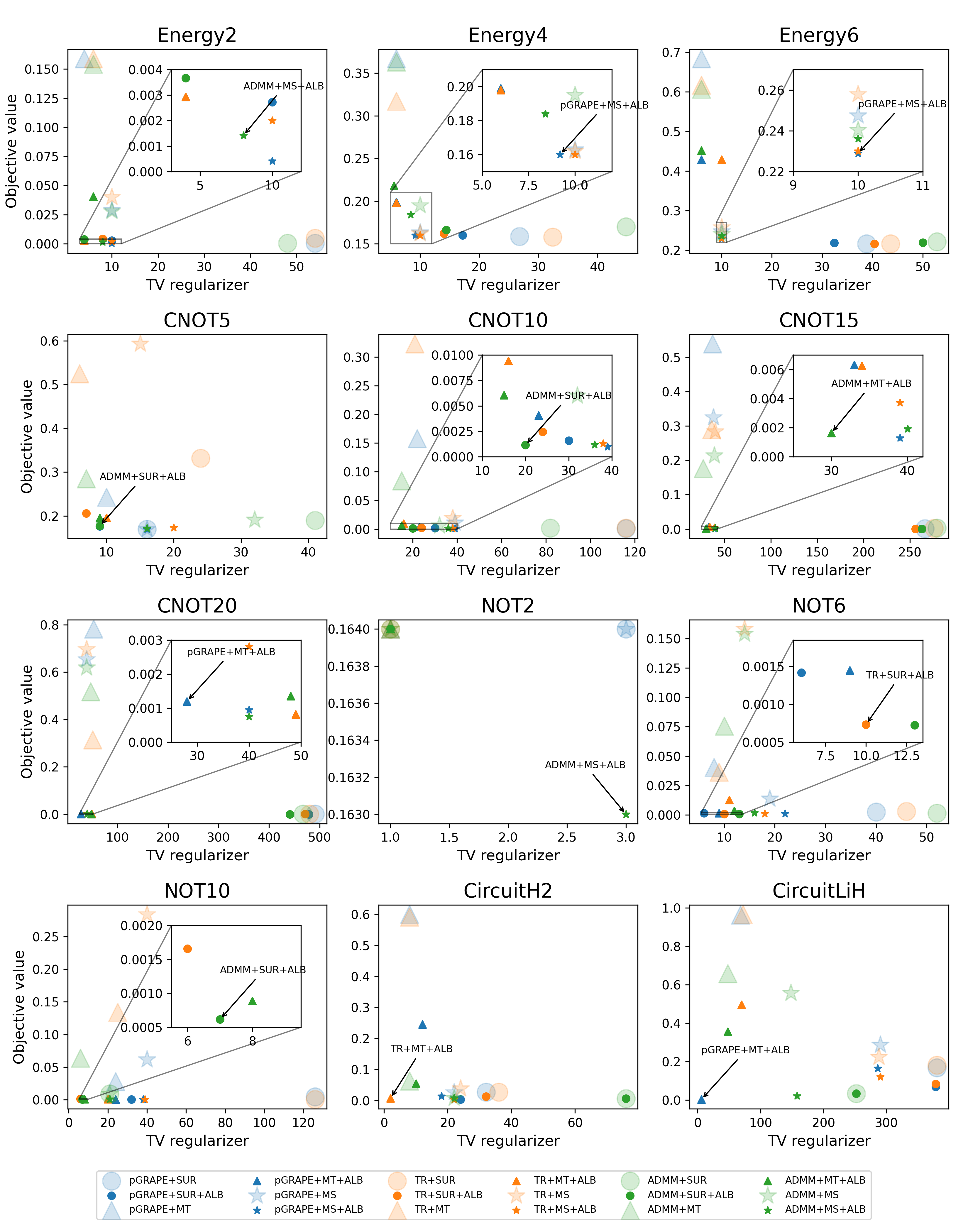
Appendix C Control Results of NOT Estimation Problem
For the NOT gate estimation problem, we present the control obtaining the best trade-off between objective values and TV regularizer values which are annotated in Figure 14. All three instances show that controller 1 has a more significant impact on the final infidelity. When the evolution time is short (), the optimal control sets controller 1 active all the time. When the evolution time is longer (), the active time of controller 2 is shorter. The main reason is that only considering controller 1 can also obtain low infidelity with a sufficiently long evolution time but the performance of a single controller is worse than two controllers with the same evolution time [86, 49].
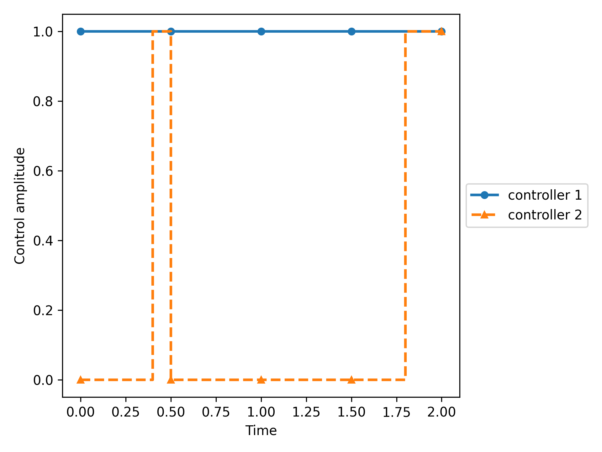
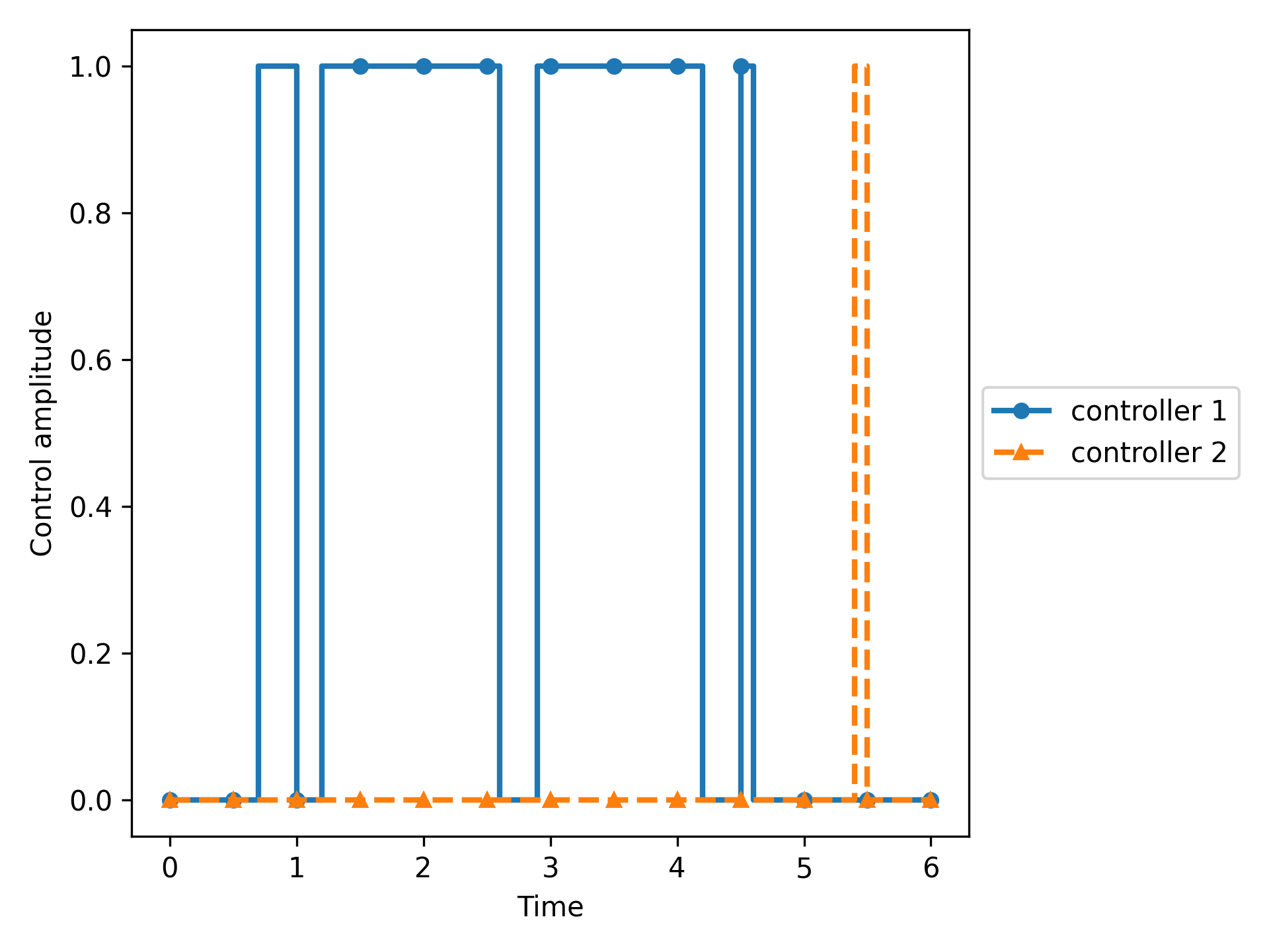
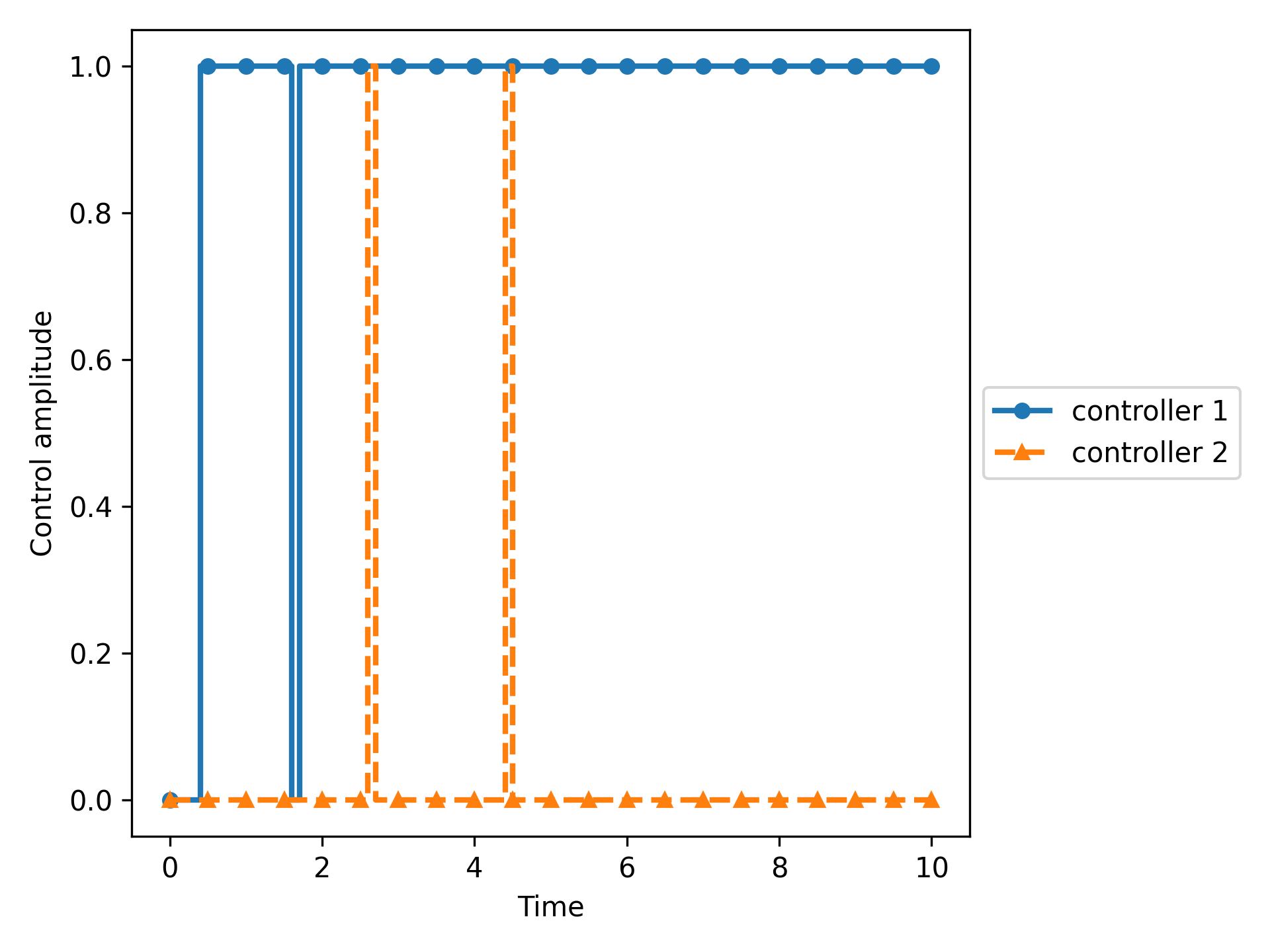
The submitted manuscript has been created by UChicago Argonne, LLC, Operator of Argonne National Laboratory (“Argonne”). Argonne, a U.S. Department of Energy Office of Science laboratory, is operated under Contract No. DE-AC02-06CH11357. The U.S. Government retains for itself, and others acting on its behalf, a paid-up nonexclusive, irrevocable worldwide license in said article to reproduce, prepare derivative works, distribute copies to the public, and perform publicly and display publicly, by or on behalf of the Government. The Department of Energy will provide public access to these results of federally sponsored research in accordance with the DOE Public Access Plan http://energy.gov/downloads/doe-public-access-plan.