Noise-induced dynamical localization and delocalization

Abstract

We investigate the effect of a two-level jump process or random telegraph noise on a square wave driven tight-binding lattice. In the absence of the noise, the system is known to exhibit dynamical localization for specific ratios of the amplitude and the frequency of the drive. We obtain an exact expression for the probability propagator to study the stability of dynamical localization against telegraph noise. Our analysis shows that in the presence of noise, a proper tuning of the noise parameters destroys dynamical localization of the clean limit in one case, while it induces dynamical localization in an otherwise delocalized phase of the clean model. Numerical results help verify the analytical findings. A study of the dynamics of entanglement entropy from an initially half-filled state offers complementary perspective.

I Introduction

A charged particle subjected to a static electric field together with a periodic lattice potential performs bounded and oscillatory motion, which is termed as Bloch oscillations  Zener (1934); Wannier (1960); Krieger and Iafrate (1986); Domínguez-Adame (2010). Here the usual Bloch band structure of a crystal lattice is destroyed and instead, we have an equispaced energy spectrum termed as the Wannier-Stark ladderHartmann et al. (2004); Gong et al. (2005). Moreover, all the single-particle wavefunctions are localized and therefore the name ‘Wannier-Stark (WS) localization’ is associated with this phenomenon. Bloch oscillations have been realized in a wide variety of physical systems such as trapped cold atoms Ben Dahan et al. (1996); Niu et al. (1996), semiconductor superlattices  Lyssenko et al. (1997); Waschke et al. (1993), photonic systems Sapienza et al. (2003); Pertsch et al. (1999), and spin systems using a superconducting quantum processor Guo et al. (2021). Furthermore, in the presence of nearest-neighbor interactions, the system exhibits many-body (Stark) localization Schulz et al. (2019); Taylor et al. (2020); Bhakuni and Sharma (2020a). The existence of Stark MBL has been probed experimentally and theoretically in recent works Guo et al. (2020); Morong et al. (2021); Taylor et al. (2020). In the presence of a time-dependent electric field, the periodic drive at specific ratios of drive amplitude and frequency $\left(A/\omega\right)$ effectively suppresses the hopping strength and leads to dynamical localization Gong et al. (2005); Lenz et al. (2003); Dunlap and Kenkre (1986); Grossmann et al. (1991); van Nieuwenburg et al. (2019); Luitz et al. (2017). Moreover, the combined action of ac and dc electric fields gives rise to fascinating phenomena like coherent destruction of WS localization Holthaus et al. (1995a, b); Bhakuni and Sharma (2018) and super Bloch oscillations Longhi and Della Valle (2012); Caetano and Lyra (2011); Kudo and Monteiro (2011) in the non-interacting limit, and coherent destruction of Stark MBL in the interacting limit Bhakuni et al. (2020). Furthermore, a coupling to bosonic heat bath (with Ohmic dissipation) leads to decoherence of the Bloch oscillations and gives rise to a dissipative transport Bandyopadhyay and Dattagupta (2021).

In a realistic situation, the system is almost always coupled to a thermalizing bath; moreover the unwanted temporal fluctuations in the drive can lead to aperiodicity, which eventually leads to dephasing and may destroy some of the above carefully-tuned properties. Such noise either originates from the lattice vibrations where the phonons are randomly excited or arises due to the fluctuations in the battery Entin-Wohlman et al. (2017); Aharony et al. (2010); Dattagupta (2012). When the electric field is static, this noise is associated with many interesting features such as incoherent destruction of WS localization and renormalization of the Bloch frequency Bhakuni et al. (2019); Bandyopadhyay et al. (2020) in the non-interacting limit, and the dephasing of Stark-MBL in the interacting case Wu and Eckardt (2019). In this work, we analyze a model in which a periodic electric field is subjected to a two-level jump process or telegraph noise. In particular, we investigate the effect of temporal noise on dynamical localization.

The main findings of our work are as follows. For a system subjected to a (telegraph) noisy time-periodic (square wave) electric field, we obtain an exact expression for the probability propagator $\tilde{\mathcal{P}}_{n}\left(t\right)$. In the clean limit, the well known case of Bloch oscillations and dynamical localization are verified for a static and periodic field respectively. Moreover, we generalize the results for a combined ac and dc field and provide an exact expression for the probability propagator leading to the cases of coherent-destruction of WS localization and super-Bloch oscillations. The rapid relaxation limit of the stochastic field is a particular focus of our work. Denoting the bias in the probabilities of the two levels of the field to be $\delta p$, we show that in the zero bias case $\left(\delta p=0\right)$, for small values of noise, dynamical localization survives. However in the long time limit and for large values of noise, we observe that noise decoheres the system by destroying dynamical localization. With a suitably chosen non-zero bias ($\delta p\neq 0$), we find that the noisy field can destroy dynamical localization yielding a delocalized phase. On the other hand, there is a way to tune the noise such that it induces dynamical localization in an otherwise delocalized phase of the clean system. A study of the entanglement entropy in the many-body setting provides useful signatures for all these effects. We corroborate our analytical calculation with an exact numerical approach by a study of the probability propagator and the dynamics of entanglement entropy.

We have organized our work as follows. In Section (II), we introduce the model Hamiltonian along with the unitary transformation to obtain an effective Hamiltonian. In Section (III), we derive the expression for the probability propagator $\tilde{\mathcal{P}}_{n}\left(t\right)$ and provide a brief discussion. The clean limit of the problem is discussed in Section (IV), while Section (V) is devoted to the case of stochastic noise. Finally, we have summarized our main findings in Section (VI).

II MODEL HAMILTONIAN

We consider the dynamics of a single-particle moving in a one dimensional tight binding chain under the influence of a time-dependent field comprising of a square wave electric field and time dependent random telegraph noise. The model Hamiltonian can be written as:

$$H = -\frac{\Delta}{4}\left(\sum_{n=-\infty}^{\infty}|n+1\rangle\langle n|+|n\rangle\langle n+1|\right)+$$ (1)

$$\mathcal{F}\left(t\right)\sum_{n=-\infty}^{\infty}n|n\rangle\langle n|,$$

where $|n\rangle$ is a Wannier state localized at site $n$ and $\Delta$ is the hopping strength. $\mathcal{F}\left(t\right)$ is the time dependent field: $\mathcal{F}\left(t\right)=F\left(t\right)+\xi\left(t\right)$, where $F\left(t\right)$ is the square wave electric field and $\xi\left(t\right)$ is a time-dependent stochastic telegraph noise. The square wave drive can be expressed as

$$F\left(t\right)=\left\{\begin{array}[]{cc}+A,&0\leq t\leq T/2\\ -A,&T/2<t\leq T\end{array}\right.,$$ (4)

where $T$ is the time period of the drive. We work in units where $\hbar=e=1$ and the lattice constant too is unity.

To study the dynamical evolution, we start by defining the unitary operators Hartmann et al. (2004):

$$\hat{K} = \sum_{n=-\infty}^{n=\infty}|n\rangle\langle n+1|$$

$$\hat{K}^{\dagger} = \sum_{n=-\infty}^{n=\infty}|n+1\rangle\langle n|$$

$$\hat{N} = \sum_{n=-\infty}^{\infty}n|n\rangle\langle n|.$$ (5)

These operators are diagonal in the quasi-momentum basis $k$:

$$\langle k^{\prime}|\hat{K}|k\rangle = e^{ik}\delta\left(k-k^{\prime}\right),$$

$$\langle k^{\prime}|\hat{K^{\dagger}}|k\rangle = e^{-ik}\delta\left(k-k^{\prime}\right),$$ (6)

and follow the commutation relations:

$$\left[\hat{K},\hat{N}\right]=\hat{K}, \left[\hat{K}^{\dagger},\hat{N}\right]=-\hat{K}^{\dagger}, \left[\hat{K},\hat{K}^{\dagger}\right]=0.$$ (7)

In terms of these unitary operators, the Hamiltonian (1) can be written as $\hat{H}=V_{+}+H_{0}\left(t\right)$, where

$$V_{+}=-\frac{\Delta}{4}\left(\hat{K}+\hat{K}^{\dagger}\right),\ \ \ H_{0}\left(t\right) = \mathcal{F}\left(t\right)\hat{N}.$$ (8)

The equation of motion for the density matrix in the Heisenberg picture is

$$\frac{d\rho}{dt} = -i\left[H\left(t\right),\rho\right].$$ (9)

After the unitary transformation, we can write the density matrix $\rho\left(t\right)$ as

$$\tilde{\rho}\left(t\right) = e^{i\int_{0}^{t}H_{0}\left(t^{\prime}\right)dt^{\prime}}\rho\left(t\right)e^{-i\int_{0}^{t}H_{0}\left(t^{\prime}\right)dt^{\prime}}.$$ (10)

Following the procedure of Bhakuni et al Bhakuni et al. (2019), we obtain the density operator in the momentum basis as

$$\langle k\mid\tilde{\rho}\left(t\right)\mid k^{\prime}\rangle = e^{-i\int_{0}^{t}\tilde{V}_{+k}\left(t^{\prime}\right)dt^{\prime}}\langle k\mid 0\rangle\langle 0\mid k^{\prime}\rangle e^{i\int_{0}^{t}\tilde{V}_{+k}\left(t^{\prime}\right)dt^{\prime}},$$

where, $\tilde{V}_{+k}\left(t^{\prime}\right)=-\frac{\Delta}{4}\left[e^{i\left(k+\eta\left(t^{\prime}\right)\right)}+e^{-i\left(k+\eta\left(t^{\prime}\right)\right)}\right]$. This suggests that the dynamical evolution of the system is governed by an effective Hamiltonian $\tilde{V}_{+k}$ where the time-dependence comes only as a phase factor. Furthermore the effective Hamiltonian respects translation invariance and hence allows us to calculate the dynamical evolution of the observables analytically as described ahead.

III Observables

In order to study the dynamics of single particle, we derive an expression for probability propagator. The probability propagator $\mathcal{P}_{n}\left(t\right)$ is a measure of the probability of finding the particle at site $n$ at a time $t$. Here, we consider an initial state where the particle is localized at the central site ($n=0$). The probability propagator can be defined as Bhakuni et al. (2019):

$$\mathcal{P}_{n}\left(t\right) = \int_{-\pi}^{\pi}\int_{-\pi}^{\pi}dk\ dk^{\prime}\langle n\mid k\rangle\langle k\mid\tilde{\rho}\left(t\right)\mid k^{\prime}\rangle\langle k^{\prime}\mid n\rangle.$$ (12)

Using Eq.(II), we can write

$$\mathcal{P}_{n}\left(t\right) = \left(\frac{1}{2\pi}\right)^{2}\int_{-\pi}^{\pi}dk\int_{-\pi}^{\pi}dk^{\prime}e^{-i\left(k-k^{\prime}\right)n}\times$$ (13)

$$e^{-i\int_{0}^{t}dt^{\prime}\left[\tilde{V}_{+k}\left(t^{\prime}\right)-\tilde{V}_{+k^{\prime}}\left(t^{\prime}\right)\right]}.$$

In our case, the time dependent field is a combination of square wave pulse and time dependent telegraph noise Yuzhelevski et al. (2000). The noise consists of random jumps between two levels $\pm\mu$. By denoting $\sigma$ and $\tau$ to be the rate of switching from level $+\mu$ to $-\mu$ and $-\mu$ to $+\mu$, respectively, the probability of being at any time in state $+\mu$ can be defined as: $p_{+}=\frac{\tau}{\lambda}$, whereas the probability of being in state $-\mu$ is: $p_{-}=\frac{\sigma}{\lambda}$ where we define $\lambda=\sigma+\tau$.

For such noise, the overall field can be expressed as a sum of $2\times 2$ matrices Blume (1968):

$$i\eta\left(t\right)=i\int_{0}^{t}F(t^{\prime})dt^{\prime}\mathcal{I}+it\mu\sigma_{z}+tW.$$ (14)

Here, $W$ is the relaxation matrix defined as Aharony et al. (2010); Dattagupta (2012)

$$W=\begin{bmatrix}-p_{-}&p_{+}\\ p_{-}&-p_{+}\\ \end{bmatrix}=\lambda\begin{bmatrix}-\frac{\sigma}{\tau+\sigma}&\frac{\tau}{\tau+\sigma}\\ \frac{\sigma}{\tau+\sigma}&-\frac{\tau}{\tau+\sigma}\end{bmatrix}$$ (15)

and $\mathcal{I}$ is the identity matrix. From Eq.(15), the relaxation matrix $W$ can be expressed as a linear combination of the identity matrix $\mathcal{I}$ and Pauli matrices $\sigma_{i}^{\prime}s$ having components $h_{0}=-h_{1}=-\gamma,h_{2}=i\delta p\gamma,h_{3}=\left(\gamma\delta p+i\mu\right)$, where $\gamma=\frac{\sigma+\tau}{2}=\frac{\lambda}{2}$, $\delta p$ is the difference between the probabilities and equals $\left(p_{+}-p_{-}\right)$.

To proceed with the calculation of the probability propagator, we express the exponential of Eq.(14) in compact form as :

$$e^{i\eta\left(t^{\prime}\right)} = e^{i\sum_{l=1}^{\infty}\alpha_{l}\left(1-\cos\left(\omega\left(2l-1\right)t^{\prime}\right)\right)}e^{-\gamma t^{\prime}}\frac{1}{2}\left[e^{\nu t^{\prime}}\left(1+\hat{h}.\vec{\sigma}\right)+\right.$$ (16)

$$\left.e^{-\nu t^{\prime}}\left(1-\hat{h}.\vec{\sigma}\right)\right],$$

where $\alpha_{l}=\frac{4AT}{2\left(2l-1\right)^{2}\pi^{2}},\ \omega=\frac{2\pi}{T}$, $l$ is an integer and $\nu=\sqrt{h_{1}^{2}+h_{2}^{2}+h_{3}^{2}}$. Here, we have exploited the identity satisfied by Pauli matrices: $e^{i\left(\vec{a}\vec{\sigma}\right)}=\left(\mathcal{I}\cos(|\textbf{a}|)+i\left(\hat{a}.\vec{\sigma}\right)\sin\left(|\textbf{a}|\right)\right)$.

Expressing the square wave in terms of its Fourier series components, Eq.(16) can be written as:

$$e^{i\eta\left(t^{\prime}\right)} = \left\{\begin{array}[]{cc}\frac{1}{2}e^{\left(iAt^{\prime}-iAnT\right)}e^{-\gamma t^{\prime}}\left[e^{\nu t^{\prime}}\left(1+\hat{h}.\vec{\sigma}\right)+\right.\\ \left.e^{-\nu t^{\prime}}\left(1-\hat{h}.\vec{\sigma}\right)\right],\\ \left(2n\pi\leq\omega t^{\prime}\leq\left(2n+1\right)\pi\right);\\ \frac{1}{2}e^{-iAt^{\prime}+iA\left(n+1\right)T}e^{-\gamma t^{\prime}}\left[e^{\nu t^{\prime}}\left(1+\hat{h}.\sigma\right)+\right.\\ \left.e^{-\nu t^{\prime}}\left(1-\hat{h}.\vec{\sigma}\right)\right],\\ \left(\left(2n+1\right)\pi<\omega t^{\prime}\leq 2\left(n+1\right)\pi\right).\end{array}\right.$$ (20)

After detailed calculations (See Appendix A), we obtain an expression for the probability propagator:

$$\mathcal{P}_{n}\left(t\right)=\left(\frac{1}{2\pi}\right)^{2}\int_{-\pi}^{\pi}dk\int_{-\pi}^{\pi}dk^{\prime}e^{-i\left(k-k^{\prime}\right)n}e^{ig_{0}\left(t\right)}$$

$$\times\left(\mathcal{I}\cos\left(|\textbf{H}|\right)+i\left(\hat{\textbf{H}}.\vec{\sigma}\right)\sin\left(|\textbf{H}|\right)\right),$$ (22)

where we have defined $H_{x}=g_{1}(t),H_{y}=g_{2}\left(t\right)=i\delta pg_{1}\left(t\right),H_{z}=g_{3}\left(t\right)=\delta pg_{1}\left(t\right)+\beta\left(t\right)$ and $g_{0}(t),g_{1}(t),g_{2}(t)$ and $g_{3}(t)$ are defined in Appendix (A). The final expression for average probability can be obtained by calculating $\tilde{\mathcal{P}}_{n}\left(t\right)=\sum_{ab}p_{a}\langle b|\mathcal{P}_{n}\left(t\right)|a\rangle$. This requires an average of various Pauli matrices with respect to the available stochastic states $|+\rangle=\begin{bmatrix}1\\ 0\end{bmatrix}$ and $|-\rangle=\begin{bmatrix}0\\ 1\end{bmatrix}$. In order to study the dynamics of the system, we use two observables: probability propagator to explore the single-particle dynamics and entanglement entropy to explore the features of a noninteracting many-fermion quantum system. This results in $\langle\sigma_{x}\rangle=1,\langle\sigma_{y}\rangle=-i\delta p,\langle\sigma_{z}\rangle=\delta p$, and $\langle\mathcal{I}\rangle=1$. With this simplification, we get the final expression of the probability propagator as

$$\tilde{\mathcal{P}}_{n}\left(t\right)=\left(\frac{1}{2\pi}\right)^{2}\int_{-\pi}^{\pi}dk\int_{-\pi}^{\pi}dk^{\prime}e^{-i\left(k-k^{\prime}\right)n}e^{ig_{0}\left(t\right)}\times\qquad\qquad$$

$$\left(\cos\left(|\textbf{H}|\right)+i\frac{g_{1}\left(t\right)}{|\textbf{H}|}\sin\left(|\textbf{H}|\right)+i\sin\left(|\textbf{H}|\right)\frac{\delta p\beta\left(t\right)}{|\textbf{H}|}\right).\qquad$$ (23)

Hence, we manage to obtain an exact expression for the probability propagator valid for both ac and dc electric fields in the presence of a telegraph noise.

To explore the effect of noisy drive in the (non-interacting) many body state, we have also calculated von-Neumann entanglement entropy (70) between two halves of the chain. For the dynamical evolution, we take the initial state $|\Psi_{in}\rangle$ where all the particles are localized to the left side of the chain

$$|\Psi_{in}\rangle=c_{1}^{\dagger}c_{2}^{\dagger}....c_{N/2}^{\dagger}|0\rangle,$$ (24)

where $c_{i}^{\dagger}$ is the creation operator at site $i$. To study the dynamics of entanglement entropy, we form a time-dependent correlation matrix Peschel (2003); Roy and Sharma (2018) as

$$C_{mn}\left(t\right) = \langle\Psi_{in}\left(t\right)|c_{m}^{\dagger}c_{n}|\Psi_{in}\left(t\right)\rangle$$ (25)

$$=\langle\Psi_{in}\left(0\right)|c_{m}^{\dagger}\left(t\right)c_{n}\left(t\right)|\Psi_{in}\left(0\right)\rangle,$$

which can be simplified to

$$C\left(t\right)=U^{\dagger}\left(t\right)C\left(0\right)U\left(t\right),$$ (26)

where $U_{jk}\left(t\right)=\sum_{n}D_{jn}^{*}\exp\left(-i\epsilon_{n}t\right)D_{nk}$ and the matrix $D$ diagonalizes the final Hamiltonian. The detailed calculation to obtain entanglement entropy from the correlation matrix is given in Appendix C. Diagonalizing the time-dependent correlation matrix and invoking Eq.(72), we can study the dynamics of entanglement entropy.

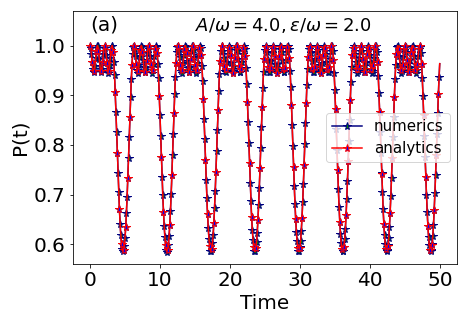
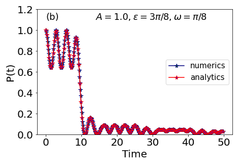
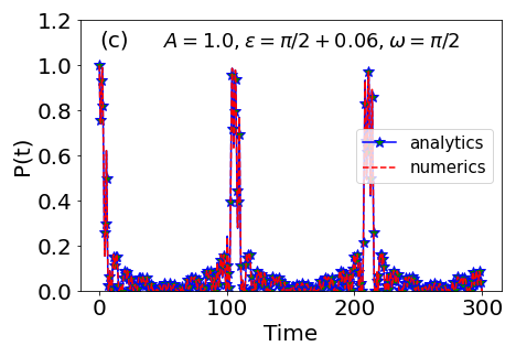
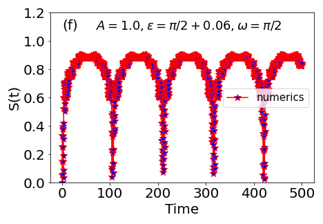
Figure 1: (a-c) Return probability for AC+DC driven system. (a) Dynamical localization for resonantly tuned DC drive ($\epsilon=n^{\prime}\omega$,with $n^{\prime}$ even). (b) Coherent destruction of Wannier-Stark localization at values away from the dynamical localization conditions. (c) Super Bloch oscillations at slightly detuned DC drive ($\epsilon=\left(n^{\prime}+\delta\right)\omega$). (d-f) Entanglement entropy for AC+DC driven system. (d) Periodicity signifies dynamical localization for resonantly tuned DC drive ($\epsilon=n^{\prime}\omega$). (e) Unbounded growth signifies delocalization at values away from dynamical localization conditions. (f) Periodic oscillations correspond to super Bloch oscillations. The other parameters are $L=200,\Delta=2.0$.

IV The driven clean system

Having obtained the exact expression for the probability propagator, we now proceed to discuss different forms of the electric field, and the various phenomena associated with them. We first consider the case where the noise is absent $\left(\mu=0\right)$ and the system is driven by a time-periodic square wave pulse. In this limit $\nu\rightarrow\gamma$ and $\beta\rightarrow 0$, and Eq.(III) becomes

$$\tilde{\mathcal{P}}_{n}\left(t\right)=\left(\frac{1}{2\pi}\right)^{2}\int_{-\pi}^{\pi}dk\int_{-\pi}^{\pi}dk^{\prime}e^{-i\left(k-k^{\prime}\right)n}e^{ig_{0}\left(t\right)}e^{ig_{1}\left(t\right)}.\qquad$$ (27)

where $g_{0}(t)$ and $g_{1}(t)$ are defined in the Appendix (Eq.(50) and (51)). For the case of a pure noise-free square wave drive (Eq. 4), we have (as shown in the Appendix):

$$\lim_{\mu\rightarrow 0}\left(g_{0}\left(t\right)+g_{1}\left(t\right)\right) = \frac{\Delta}{2A}\left\{\frac{\left(t-\tau\right)}{\pi/\omega}\left(\sin\left(k+\pi A/\omega\right)\right.\right.$$ (28)

$$\left.\left.-\sin k\right)+\left(\sin\left(k+A\tau\right)-\sin k\right)-\right.$$

$$\left.\frac{\left(t-\tau\right)\omega}{\pi}\left(\sin\left(k^{\prime}+\pi A/\omega\right)-\sin k^{\prime}\right)\right.$$

$$\left.-\left(\sin\left(k^{\prime}+A\tau\right)-\sin k^{\prime}\right)\right\},$$

where $t=mT+\tau,\quad\left(0<\tau<T/2\right)$ and $m$ is a positive integer. In the limit $\omega\to 0$, we have a static field, and it is evident that only the second and fourth terms in Eq(28) survive, and yield the familiar Bloch oscillations. For nonzero $\omega$, we observe that Eq(28) becomes a periodic function with period $\frac{2\pi}{A}$ if the ratio $\frac{A}{\omega}$ is tuned to an even integer. This periodicity corresponds to dynamical localization at these specific ratios of the amplitude and frequency as reported previously Luitz et al. (2017); Eckardt et al. (2009). On the other hand, going away from these special points, for $A/\omega=$odd integer, we have

$$\lim_{\mu\rightarrow 0}\left(g_{0}\left(t\right)+g_{1}\left(t\right)\right) = \left\{\frac{\Delta\zeta}{A}\left(\sin\left(-C+k\right)\right)\right.$$ (29)

$$\left.-\frac{\Delta\zeta}{A}\left(\sin\left(-C+k^{\prime}\right)\right)\right\},$$

where $\zeta=\sqrt{\frac{\left(t-\tau\right)^{2}}{\pi^{2}/\omega^{2}}+\sin^{2}A\tau},\cos C=\frac{\left(t-\tau\right)}{\zeta\pi/\omega},\sin C=\frac{\sin A\tau}{\zeta}$. This gives a closed-form expression for the probability propagator:

$$\tilde{\mathcal{P}}_{n}\left(t\right) = \left(J_{0}\left(\Delta\zeta/A\right)\right)^{2},$$ (30)

which suggests a decaying behavior in time and hence signifies the delocalization of an initially localized wave-packet.

Another interesting case arises when the electric field has both ac and dc parts. Numerical and semi-classical studies Bhakuni et al. (2020); Bhakuni and Sharma (2018) on such combined ac and dc electric fields have revealed several interesting phenomena such as coherent destruction of Wannier-Stark localization, dynamical localization, and super-Bloch oscillations. Here, we discuss these phenomena in the backdrop of our exact result for the probability propagator. When the system is subjected to a square wave drive with amplitude $A$ and frequency $\omega$ along with a uniform dc field $\epsilon$ i.e. $\mathcal{F}\left(t\right)=F\left(t\right)+\epsilon$,  Eq.(28) gets modified to:

$$\lim_{\mu\rightarrow 0}\left(g_{0}\left(t\right)+g_{1}\left(t\right)\right) = \lim_{\mu\rightarrow 0}\frac{\Delta}{4}\left[\left(z-z^{\prime}\right)\left\{\left(\frac{1-e^{-\left(-i\epsilon-iA\right)\pi/\omega}}{\left(-i\epsilon-iA\right)}+\frac{\left(1-e^{-\left(-i\epsilon+iA\right)\pi/\omega}\right)e^{-\left(-i\epsilon+iA\right)\pi/\omega}e^{iA.2\pi/\omega}}{\left(-i\epsilon+iA\right)}\right)\right.\right.$$ (31)

$$\left.\left.\left(\frac{1-e^{-\left(\gamma-\nu-i\epsilon\right)2m\pi/\omega}}{1-e^{-\left(\gamma-\nu-i\epsilon\right)2\pi/\omega}}\right)+\frac{e^{i\epsilon\frac{2m\pi}{\omega}}\left(1-e^{-\left(-i\epsilon-iA\right)\left(\tau\right)}\right)}{\left(-i\epsilon-iA\right)}\right\}+c.c.\right]$$

where $z=e^{ik},z^{\prime}=e^{ik^{\prime}}$, which in turn leads to

$$\lim_{\mu\rightarrow 0}\left(g_{0}\left(t\right)+g_{1}\left(t\right)\right) = \frac{\Delta}{2}\left\{\frac{\left(t-\tau\right)}{\left(A+\epsilon\right)\frac{2\pi}{\omega}}\left[\left(\sin\left(k+\pi\left(A+\epsilon\right)/\omega\right)-\sin k\right)-\left(\sin\left(k^{\prime}+\pi\left(A+\epsilon\right)/\omega\right)-\sin k^{\prime}\right)\right]\right.$$ (32)

$$\left.+\frac{\left(t-\tau\right)}{\left(A-\epsilon\right)\frac{2\pi}{\omega}}\left[\left(\sin\left(k+\pi\left(A+\epsilon\right)/\omega\right)-\sin\left(k+\frac{2\epsilon\pi}{\omega}\right)\right)-\left(\sin\left(k^{\prime}+\pi\left(A+\epsilon\right)/\omega\right)-\right.\right.\right.$$

$$\left.\left.\left.\sin\left(k^{\prime}+\frac{2\epsilon\pi}{\omega}\right)\right)\right]+\frac{1}{\left(A+\epsilon\right)}\left[\sin\left(k+\left(A+\epsilon\right)\tau+\frac{2m\epsilon\pi}{\omega}\right)-\sin\left(k+\frac{2m\epsilon\pi}{\omega}\right)\right]\right.$$

$$\left.-\frac{1}{\left(A+\epsilon\right)}\left[\sin\left(k^{\prime}+\left(A+\epsilon\right)\tau+\frac{2m\epsilon\pi}{\omega}\right)-\sin\left(k^{\prime}+\frac{2m\epsilon\pi}{\omega}\right)\right]\right\}.$$

Eq.(32) suggests that certain special ratios of the static field with the frequency of the square wave drive may yield interesting dynamical phenomena. For $A/\omega=2n$, we see periodic behavior if the static field is tuned at $\epsilon/\omega=2n^{\prime},\left(n\neq n^{\prime}\right)$. This corresponds to dynamical localization as shown in Fig.(1)(a,d), where the initially localized wave-packet returns to its initial state after a driving period and both the probability and the entanglement entropy oscillate in time. If the static field is resonantly tuned with $\epsilon/\omega=2n^{\prime}$, but the ratio $A/\omega$ is set to be something other than an even integer, the driving leads to band formation Bhakuni et al. (2020) and destroys the localization set up by the static field. This coherent destruction of Wannier Stark localization is shown in Fig.(1)(b,e) where the probability decays in time and the entropy shows an unbounded growth despite the presence of the static field. Similarly, if the static field is resonantly tuned at $\epsilon/\omega=2n^{\prime}+1,\left(n\neq n^{\prime}\right)$, dynamical localization can again be observed if $A/\omega=2n+1$ is also an odd integer. However, while maintaining the resonance condition, if the static field is not tuned in this precise manner, we once again observe coherent destruction of Wannier-Stark localization.

Finally, when the static electric field is slightly detuned from the resonance condition such that $\epsilon=\left(n^{\prime}+\delta\right)\omega$, the phase factor in Eq. (32) acquires an extra term $\delta\omega t$ and it becomes

$$\lim_{\mu\rightarrow 0}\left(g_{0}\left(t\right)+g_{1}\left(t\right)\right) = \frac{\Delta}{2}\left[\frac{1}{\left(A+\epsilon\right)\sin(\delta\pi)}\left\{\sin\left(k^{\prime}+(m-1)\delta\pi\right)-\sin\left(k+(m-1)\delta\pi\right)\right\}\sin(m\delta\pi)+\frac{1}{\left(A-\epsilon\right)\sin(\delta\pi)}\right.$$

$$\left.\left\{\sin\left(k^{\prime}+\delta\pi+m\delta\pi\right)-\sin\left(k+\delta\pi+m\delta\pi\right)\right\}\sin(m\delta\pi)+\frac{2A}{\left(A^{2}-\epsilon^{2}\right)\sin(\delta\pi)}\right.$$

$$\left.\left\{\sin\left(k+\frac{A\pi}{\omega}+n^{\prime}\pi+m\delta\pi\right)-\sin\left(k^{\prime}+\frac{A\pi}{\omega}+n^{\prime}\pi+m\delta\pi\right)\right\}\sin\left(m\pi\delta\right)+\frac{2}{\left(A+\epsilon\right)}\right.$$

$$\left.\left\{\sin\left(k+(n^{\prime}+\delta)\omega t+A\tau\right)-\sin\left(k+m\delta\omega T\right)-\sin\left(k^{\prime}+(n^{\prime}+\delta)\omega t+A\tau\right)+\sin\left(k^{\prime}+m\delta\omega T\right)\right\}\right].$$

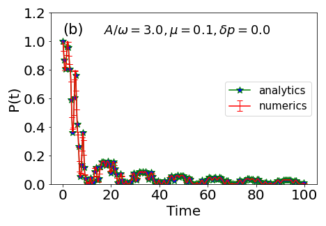
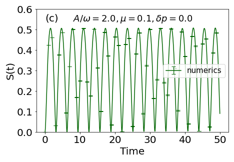
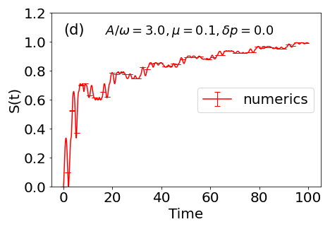
Figure 2: Data for fluctuating square wave driven system. (a) shows the periodic behavior of return probability at dynamical localization point. (b) shows decaying behavior of probability at points away from dynamical localization. (c) shows periodic behavior of entanglement entropy at dynamical localization point and (d) shows unbounded growth of entanglement entropy at points away from dynamical localization conditions. We present data for the zero bias case $\left(\delta p=0.0\right)$ in the rapid relaxation regime $\left(\sigma=100,\tau=100\right)$ with hopping strength $\Delta=2.0$. We have averaged over 200 realizations of disorder for a system of size $L=200$.

The system exhibits oscillatory behaviour similar to Bloch oscillations. Analogous to the case of the static field driven system, these oscillations are termed as super Bloch oscillations and the frequency of these oscillations is directly proportional to $\delta\omega$. This phenomenon has been shown in Fig.(1)(c,f) where return probability and entanglement entropy exhibit periodic behaviour with the frequency given by the offset.

V Effect of Stochastic Noise

In this section, we will focus on how the presence of time dependent fluctuations affect the dynamical localization in the system. We present an analytical expression for the probability propagator and also test its validity with the aid of an exact numerical approach. To simulate the telegraph noise and the dynamical protocol, we follow Bhakuni et al Bhakuni et al. (2019) and average the observables over many noise trajectories. We will restrict ourselves to the case of zero static field and discuss the effects of the inclusion of a noisy field. We consider two different cases: one where the two levels of the noise are equiprobable ($\delta p=0$) and the other where one level is more probable ($\delta p\neq 0$). While the expression for the probability propagator is general, we will restrict ourselves to the rapid relaxation regime, in order to obtain approximate expressions that are effective and simple. In this limit $\gamma>>\mu,A$ and $g_{1}\left(t\right)^{2}>>\beta\left(t\right)^{2}$. With these approximations, we can expand $|\textbf{H}|$ as

$$|\textbf{H}| = \sqrt{g_{1}\left(t\right)^{2}+\beta\left(t\right)^{2}+2\delta pg_{1}\left(t\right)\beta\left(t\right)}$$ (34)

$$\approx g_{1}\left(t\right)\left(1+\frac{\beta\left(t\right)^{2}}{2g_{1}\left(t\right)^{2}}+\frac{\delta p\beta\left(t\right)}{g_{1}\left(t\right)}\right),$$

and the expression which appears in the integrand of Eq. (III) can be approximated as

$$e^{ig_{0}\left(t\right)} \left(\cos\left(|\textbf{H}|\right)+i\frac{\sin(|\textbf{H}|)}{|\textbf{H}|}\Big{[}g_{1}\left(t\right)+\delta p\beta\left(t\right)\Big{]}\right)$$

$$\approx\exp\Big{(}i(g_{0}\left(t\right)+|\textbf{H}|)\Big{)}\qquad\qquad$$

$$\approx\exp{(ig_{0}(t)+ig_{1}(t)+i\delta p\beta(t)+i\frac{\beta^{2}(t)}{2g_{1}(t)}}).$$

First, we consider the case of zero bias $\left(\delta p=0\right)$ with zero external drive. In this limit $\nu=\sqrt{\gamma^{2}-\mu^{2}}\approx\left(\gamma-\frac{\mu^{2}}{2\gamma}\right)$. When the field is zero $\left(A=0\right)$, Eq.(V) is modified to Eq.(61) (see Appendix), which in the long-time limit, futher simplifies to

$$e^{ig_{0}\left(t\right)+ig_{1}\left(t\right)}e^{i\frac{\beta^{2}\left(t\right)}{2g_{1}\left(t\right)}} \approx e^{i\frac{\Delta_{\textsf{eff}}}{4}t\left(\cos k-\cos k^{{}^{\prime}}\right)},$$ (36)

where $\Delta_{\textsf{eff}}=\Delta\left(1+\frac{1}{2}\left(\frac{\mu}{\gamma}\right)^{2}\frac{\left(\sin k-\sin k^{\prime}\right)^{2}}{\left(\cos k-\cos k^{\prime}\right)^{2}}\right)$. This expression shows that in the zero field limit, the dynamics is governed by a renormalized hopping parameter $\Delta_{\textsf{eff}}$ for rapidly fluctuating noise, thus recovering an earlier result Bhakuni et al. (2019).

Now, we consider the square wave driven system $\left(A\neq 0\right)$. In this case, we can ignore $e^{i\frac{\beta^{2}\left(t\right)}{2g_{1}\left(t\right)}}$ and Eq.(V) is approximated to Eq.(65). In the rapid relaxation limit, for $A/\omega=2n,$ Eq.(65) further simplifies to:

$$g_{0}\left(t\right)+g_{1}\left(t\right) \approx\frac{-\Delta e^{-\frac{\mu^{2}}{2\gamma}t}}{2A}\Big{[}e^{\frac{\mu^{2}\tau}{2\gamma}}\left(\sin k-\sin k^{\prime}\right)$$

$$-\left(\sin\left(k+A\tau\right)-\sin\left(k^{\prime}+A\tau\right)\right)\Big{]}.$$ (37)

It is clear from Eq.(V) that $g_{0}\left(t\right)+g_{1}\left(t\right)$ will exhibit periodic behavior (with period $\frac{2\pi}{A}$) only for small values of noise ($\mu<<\gamma$), whereas for large values of noise and in the long time limit, the periodic oscillations damp out exponentially. The dynamics of return probability and entanglement entropy are plotted in Fig.(2). At the dynamical localization point, we see the oscillatory nature of the probability propagator (Fig. 2(a)) and the entropy (Fig. 2(c)). However these oscillations are bound to decay on much longer time scales. Similarly, when the parameters are tuned away from the dynamical localization point, we see a decaying behavior of probability and an unbounded growth of the entanglement entropy as depicted in Fig. (2)(b) and Fig. (2)(d) respectively.

We next consider the case where one level of the telegraph noise is more probable than the other i.e. $\delta p\neq 0$. In this case, we can approximate $\nu$ as: $\nu=\sqrt{\gamma^{2}-\mu^{2}+2i\mu\gamma\delta p}\approx\left(\gamma-\frac{\mu^{2}}{2\gamma}+i\mu\delta p\right)$. For $A/\omega=2n$, with this approximation and further simplifications (via Eq. (68)) we arrive at:

$$g_{0}(t)+g_{1}(t)+\delta p\beta(t) \approx \frac{-\Delta e^{-\frac{\mu^{2}}{2\gamma}t}}{2(\mu\delta p+A)}\Big{[}e^{\frac{\mu^{2}}{2\gamma}\tau}\left\{\sin(k+\mu\delta p(t-\tau))-\sin(k^{\prime}+\mu\delta p(t-\tau))\right\}-$$ (38)

$$\left\{\sin\left(k+\mu\delta pt+A\tau\right)-\sin\left(k^{\prime}+\mu\delta pt+A\tau\right)\right\}\Big{]}.$$

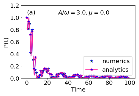
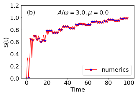
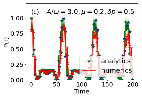
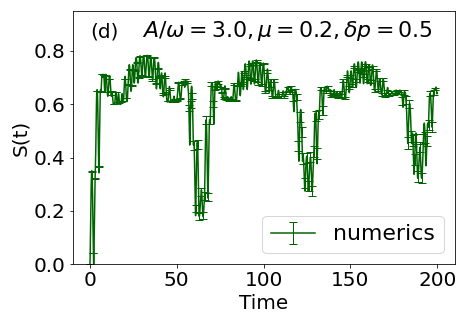
Figure 3: Return probability and entanglement entropy in the absence and the presence of noise when the ratio of the amplitude and the frequency is fixed to be an odd integer (we set $A/\omega=3$). Plots (a) and (b) show decaying behavior of return probability and unbounded growth of entanglement entropy respectively in the absence of noise. A suitable noise can help engineer ‘noise-induced’ dynamical localization as shown by the oscillatory behavior of return probability and entanglement entropy respectively in (c) and (d). The other parameters are $L=200,\Delta=4.0$. The data are averaged over $100$ realizations of disorder.

The above expression resembles Eq. (32) with the static field $\epsilon$ replaced by an effective field $\mu\delta p$. Thus we expect phenomena similar to dynamical localization and coherent destruction of Wannier-Stark localization to be induced by the noisy field. When the ratio of the amplitude to the frequency is tuned to be an odd integer ($A/\omega=\left(2n+1\right)$), the noisy field induces dynamical localization. Fig.(3) shows the probability and the entanglement entropy, for this scenario both in the absence and presence of noise. The clean limit, as seen from Fig.(3) (a,b), results in delocalization behavior. On the other hand, we see that a carefully tuned noise induces dynamical localization which is signalled by the probability and the entropy showing oscillatory behavior (Fig.(3)(c,d)). This signifies the emergence of a new kind of dynamical localization that is induced by a noisy field. As the strength of the noise is increased, the system loses coherence resulting in a transition to delocalization. It is worth pointing out that in Figs. 3(c,d), a tendency for the oscillations to decay is also visible, although these effects may become important only when very long timescales are involved.

Contrastingly, the noisy field can also lead to a complete destruction of dynamical localization when the ratio of the amplitude to the frequency is tuned to be an even integer ($A/\omega=\left(2n\right)$). As shown in Fig. (4) in the absence of the noise, the parameters of the drive lead to dynamical localization where the probability and the entropy oscillate in time (Fig. 4(a,b)). However, in the presence of an appropriately tuned noisy field, dynamical localization is destroyed and delocalization behavior is observed as shown in Fig. (4)(c,d) where the probability and the entropy exhibit decaying behavior and unbounded growth respectively. These interesting results are reminiscent of the case of a periodically driven system together with a static field in the clean limit as discussed in the previous section. However in this scenario, the effects are induced by the noisy field which on average works as a static field.

Figure 4: Plots (a) and (b) show oscillatory behavior of return probability and entanglement entropy corresponding to dynamical localization for a clean system with the tuning $\left(A/\omega=2n\right)$. When a suitably tuned noise is included delocalization behaviour can be induced as signalled by the decaying nature of the probability and unbounded growth of entanglement entropy in (c) and (d) respectively. We have averaged over $145$ realizations of disorder for a system of size $L=200$. The hopping strength is set to $\Delta=2.0$.

VI Summary and Conclusion

To summarize, we study the dynamics under a noisy electric field and examine how the phenomenon of dynamical localization in the clean limit gets affected by the noisy field. We obtain an exact expression for the probability propagator for a generalized field including a static part, a time-periodic part, and a noisy part modeled by telegraph noise. In the clean limit, we discuss the phenomena of dynamical localization, coherent destruction of Wannier-Stark localization, and super-Bloch oscillations with the help of the obtained probability propagator.

In the presence of noise, we show that the dynamical localization survives for small noise strength for some time and damps out in the long time limit, while a larger value of the noisy field brings decoherence to the system causing the delocalization of the particle. When the two levels of the noise are not equi-probable, we observe two interesting effects. In one case, with a proper tuning of the ratio of the amplitude and the driving frequency, dynamical localization can be destroyed incoherently, while with a different tuning of the ratio of the amplitude and the driving frequency, we see the emergence of dynamical localization induced by the noisy field. Thus with a suitable tuning of the noise parameters, we are able to go from a dynamically localized phase to a delocalized one and vice-versa.

It is known that the clean limit of an interacting driven model can exhibit exciting phenomena such as drive induced many-body localization Bairey et al. (2017); Bhakuni et al. (2020) and coherent destruction of Stark-many-body localization Bhakuni et al. (2020); Bhakuni and Sharma (2020b). Thus, it would be interesting to investigate the interplay of many-body interactions, drive and noise to check if further noise-induced effects can be engineered. Another possibility for exploration would be to consider other forms of noise, which have been studied recently Bandyopadhyay et al. (2020).

Appendix A

CALCULATION OF PROBABILITY PROPAGATOR

Beginning with the expression for the probability propagator (Eq.(13)):

$$\mathcal{P}_{n}\left(t\right) = \left(\frac{1}{2\pi}\right)^{2}\int_{-\pi}^{\pi}dk\int_{-\pi}^{\pi}dk^{\prime}e^{-i\left(k-k^{\prime}\right)n}\times e^{-i\int_{0}^{t}dt^{\prime}\left[\tilde{V}_{+k}\left(t^{\prime}\right)-\tilde{V}_{+k^{\prime}}\left(t^{\prime}\right)\right]},$$

we will show how to obtain Eq.(III). To caclulate the integral that appears in the exponential of the integrand of Eq.(13), it is helpful to recall Eq.(II):

$$e^{-i\int_{0}^{t}dt^{\prime}[V_{k}^{+}(t^{\prime})-V_{k^{\prime}}^{+}(t^{\prime})]} = e^{\frac{-i\Delta}{4}\int_{0}^{t}dt^{\prime}\left[\left\{e^{i(k+\eta(t^{\prime}))}+c.c.\right\}-\left\{e^{i(k^{\prime}+\eta(t^{\prime}))}+c.c.\right\}\right]},$$ (39)

where

$$e^{i\eta\left(t^{\prime}\right)} = \left\{\begin{array}[]{cc}\frac{1}{2}e^{\left(iAt^{\prime}-iAnT\right)}\left[e^{(\nu-\gamma)t^{\prime}}\left(1+\hat{h}.\vec{\sigma}\right)+e^{-(\nu+\gamma)t^{\prime}}\left(1-\hat{h}.\vec{\sigma}\right)\right];\quad\left(2n\pi\leq\omega t^{\prime}\leq\left(2n+1\right)\pi;\quad n=0,1,2..\right)\\ \frac{1}{2}e^{-iAt^{\prime}+iA\left(n+1\right)T}\left[e^{(\nu-\gamma)t^{\prime}}\left(1+\hat{h}.\sigma\right)+e^{-(\nu+\gamma)t^{\prime}}\left(1-\hat{h}.\vec{\sigma}\right)\right];\quad\left(\left(2n+1\right)\pi<\omega t^{\prime}\leq 2\left(n+1\right)\pi\right).\end{array}\right.$$ (41)

Next, to simplify Eq.(39), we consider the following possibilities for a finite time $t$:

1. $t=mT+\tau$,

2. $t=mT+\frac{T}{2}+\tau$,

where $0<\tau<\frac{T}{2}$ and $m$ is a non-zero positive integer. Now, we present here our calculation for $t=mT+\tau$ and later will generalize it for a general time $t$. We have:

$$\int_{0}^{mt+\tau}dt^{\prime}e^{i\eta(t^{\prime})}=\frac{1}{2}\left[\left\{f_{1}(\nu)+f_{1}(-\nu)\right\}+\left(\hat{h}.\vec{\sigma}\right)\left\{f_{1}(\nu)-f_{1}(-\nu)\right\}\right],$$ (43)

where

$$f_{1}(\nu) = \left\{\left(\frac{1-e^{-\left(\gamma-\nu-iA\right)T/2}}{\left(\gamma-\nu-iA\right)}+\frac{\left(1-e^{-\left(\gamma-\nu+iA\right)T/2}\right)e^{-\left(\gamma-\nu+iA\right)T/2}e^{iAT}}{\left(\gamma-\nu+iA\right)}\right)\left(\frac{1-e^{-\left(\gamma-\nu\right)mT}}{1-e^{-\left(\gamma-\nu\right)T}}\right)\right.$$ (44)

$$\left.+\frac{e^{-\left(\gamma-\nu\right)mT}}{\left(\gamma-\nu-iA\right)}\left(1-e^{-\left(\gamma-\nu-iA\right)\left(t-mT\right)}\right)\right\}$$

and

$$f_{1}\left(-\nu\right) = \left\{\left(\frac{1-e^{-\left(\gamma+\nu-iA\right)T/2}}{\left(\gamma+\nu-iA\right)}+\frac{\left(1-e^{-\left(\gamma+\nu+iA\right)T/2}\right)e^{-\left(\gamma+\nu+iA\right)T/2}e^{iAT}}{\left(\gamma+\nu+iA\right)}\right)\left(\frac{1-e^{-\left(\gamma+\nu\right)mT}}{1-e^{-\left(\gamma+\nu\right)T}}\right)\right.$$ (45)

$$\left.+\frac{e^{-\left(\gamma+\nu\right)mT}}{\left(\gamma+\nu-iA\right)}\left(1-e^{-\left(\gamma+\nu-iA\right)\left(t-mT\right)}\right)\right\}.$$

Using Eq. (43) the exponential in the L.H.S. of Eq.(39) can be expressed as:

$$-i\int_{0}^{mt+\tau}dt^{{}^{\prime}}\left[V_{k}^{+}\left(t^{{}^{\prime}}\right)-V_{k^{{}^{\prime}}}^{+}\left(t^{{}^{\prime}}\right)\right] =\frac{i\Delta}{8}\left[\left(z-z^{\prime}\right)\left\{f_{1}\left(\nu\right)+f_{1}\left(-\nu\right)\right\}+\left(z-z^{\prime}\right)\left(\hat{h}.\vec{\sigma}\right)\left\{f_{1}\left(\nu\right)-f_{1}\left(-\nu\right)\right\}+c.c.\right],$$ (46)

where $z=e^{ik},z^{\prime}=e^{ik^{\prime}}$. To generalize, we can write the above Eq. (46) as:

$$-i\int_{0}^{t}dt^{{}^{\prime}}\left[V_{k}^{+}\left(t^{{}^{\prime}}\right)-V_{k^{{}^{\prime}}}^{+}\left(t^{{}^{\prime}}\right)\right] =\frac{i\Delta}{8}\left[\left(z-z^{\prime}\right)\left\{f_{2}\left(\nu\right)+f_{2}\left(-\nu\right)\right\}+\left(z-z^{\prime}\right)\left(\hat{h}.\vec{\sigma}\right)\left\{f_{2}\left(\nu\right)-f_{2}\left(-\nu\right)\right\}+c.c.\right].$$ (47)

where the general time $t$ can be accommodated with the aid of Heaviside step functions:

$$f_{2}(\nu) = \left\{\left(\frac{1-e^{-\left(\gamma-\nu-iA\right)T/2}}{\left(\gamma-\nu-iA\right)}+\frac{\left(1-e^{-\left(\gamma-\nu+iA\right)T/2}\right)e^{-\left(\gamma-\nu+iA\right)T/2}e^{iAT}}{\left(\gamma-\nu+iA\right)}\right)\left(\frac{1-e^{-\left(\gamma-\nu\right)mT}}{1-e^{-\left(\gamma-\nu\right)T}}\right)\right.$$

$$\left.+\frac{e^{-\left(\gamma-\nu\right)mT}}{\left(\gamma-\nu-iA\right)}\left(1-e^{-\left(\gamma-\nu-iA\right)\tau}\right)+\frac{e^{-\left(\gamma-\nu\right)mT}e^{-\left(\gamma-\nu-iA\right)T/2}}{\left(\gamma-\nu+iA\right)}\left(1-e^{-\left(\gamma-\nu+iA\right)\left(t-mT-\frac{T}{2}\right)\mathcal{H}\left(t-mT-\frac{T}{2}\right)}\right)\right\},$$

$$f_{2}\left(-\nu\right) = \left\{\left(\frac{1-e^{-\left(\gamma+\nu-iA\right)T/2}}{\left(\gamma+\nu-iA\right)}+\frac{\left(1-e^{-\left(\gamma+\nu+iA\right)T/2}\right)e^{-\left(\gamma+\nu+iA\right)T/2}e^{iAT}}{\left(\gamma+\nu+iA\right)}\right)\left(\frac{1-e^{-\left(\gamma+\nu\right)mT}}{1-e^{-\left(\gamma+\nu\right)T}}\right)+\right.$$

$$\left.\frac{e^{-\left(\gamma+\nu\right)mT}}{\left(\gamma+\nu-iA\right)}\left(1-e^{-\left(\gamma+\nu-iA\right)\tau}\right)+\frac{e^{-\left(\gamma+\nu\right)mT}e^{-\left(\gamma+\nu-iA\right)T/2}}{\left(\gamma+\nu+iA\right)}\left(1-e^{-\left(\gamma+\nu+iA\right)\left(t-mT-\frac{T}{2}\right)\mathcal{H}\left(t-mT-\frac{T}{2}\right)}\right)\right\}.$$

Here $\tau=\left\{\begin{array}[]{cc}t-mT,&\left(t-mT\right)<\frac{T}{2}\\ \frac{T}{2},&\left(t-mT\right)\geqslant\frac{T}{2}\end{array}\right.$, and the Heaviside step function is defined as: $\mathcal{H}\left(x\right)=\left\{\begin{array}[]{cc}0,&x<0\\ 1,&x\geqslant 0\end{array}\right.$. The exponential of Eq. (47) can now be written in compact form as:

$$e^{-i\int_{0}^{t}dt^{\prime}[V_{k}^{+}(t^{\prime})-V_{k^{\prime}}^{+}(t^{\prime})]} = e^{ig_{0}\left(t\right)}e^{i\left(\textbf{H}.\vec{\sigma}\right)}$$ (49)

$$= e^{ig_{0}\left(t\right)}\left(\mathcal{I}\cos\left(|\textbf{H}|\right)+i\left(\hat{\textbf{H}}.\vec{\sigma}\right)\sin\left(|\textbf{H}|\right)\right),$$

where we have used the identity $e^{i\left(\vec{a}\vec{\sigma}\right)}=\left(\mathcal{I}\cos|\textbf{a}|+i\left(\hat{a}.\vec{\sigma}\right)\sin\left(|\textbf{a}|\right)\right)$, and defined $H_{x}=g_{1}\left(t\right),H_{y}=g_{2}\left(t\right)=i\delta pg_{1}\left(t\right),H_{z}=g_{3}\left(t\right)=\delta pg_{1}\left(t\right)+\beta\left(t\right)$ and $|\textbf{H}|=\sqrt{g_{1}^{2}(t)+g_{2}^{2}(t)+g_{3}^{2}(t)}$. The functions $g_{0}(t),g_{1}(t),$ and $\beta\left(t\right)$ are given by:

$$g_{0}\left(t\right) = \frac{\Delta}{8}\left[\left(z-z^{\prime}\right)\left\{f_{2}\left(\nu\right)+f_{2}\left(-\nu\right)\right\}+c.c.\right]$$ (50)

$$g_{1}\left(t\right) = \frac{\Delta\gamma}{8}\left[\frac{\left(z-z^{\prime}\right)}{\nu}\left\{f_{2}\left(\nu\right)-f_{2}\left(-\nu\right)\right\}+c.c.\right]$$ (51)

$$\beta\left(t\right) = \frac{i\Delta\mu}{8}\left[\left(z-z^{\prime}\right)\left\{f_{2}\left(\nu\right)-f_{2}\left(-\nu\right)\right\}-c.c.\right].$$ (52)

Hence, we arrive at the expression for the probability propagator given in Eq.(III):

$$\mathcal{P}_{n}\left(t\right)=\left(\frac{1}{2\pi}\right)^{2}\int_{-\pi}^{\pi}dk\int_{-\pi}^{\pi}dk^{\prime}e^{-i\left(k-k^{\prime}\right)n}e^{ig_{0}\left(t\right)}\times\left(\mathcal{I}\cos\left(|\textbf{H}|\right)+i\left(\hat{\textbf{H}}.\vec{\sigma}\right)\sin\left(|\textbf{H}|\right)\right).$$ (53)

Appendix B

CALCULATION OF PROBABILITY PROPAGATOR FOR RAPID RELAXATION REGIME

Here, we discuss the rapid relaxation regime in which $\gamma>>\mu,A$. In this limit $\Theta^{2}(t)>>\beta^{2}(t)$, hence we can approximate $|\textbf{H}|$ as:

$$|\textbf{H}|=\sqrt{g_{1}^{2}\left(t\right)+\beta^{2}\left(t\right)+2\delta pg_{1}\left(t\right)\beta\left(t\right)}\approx g_{1}\left(t\right)\left(1+\frac{\beta^{2}\left(t\right)}{2g_{1}^{2}\left(t\right)}+\frac{\delta p\beta\left(t\right)}{g_{1}\left(t\right)}\right).$$ (54)

This implies the following simplification to the intergand of Eq.(III):

$$e^{ig_{0}\left(t\right)}\left(\cos\left(|\textbf{H}|\right)+i\frac{\sin(|\textbf{H}|)}{|\textbf{H}|}\Big{[}g_{1}\left(t\right)+\delta p\beta\left(t\right)\Big{]}\right) \approx\exp\Big{(}i(g_{0}\left(t\right)+|\textbf{H}|)\Big{)}\qquad\qquad$$

$$\approx\exp{\left(ig_{0}(t)+ig_{1}(t)+i\delta p\beta(t)+i\frac{\beta^{2}(t)}{2g_{1}(t)}\right)}.$$ (55)

Now, we consider two different cases of two-level telegraph noise based on the probability associated with both the levels in the following subsections.

B.1 Zero Bias Case $(\delta p=0)$

In this subsection, we will consider the case when both the levels of noise are equally probable i.e. the case of zero bias $\left(\delta p=0\right)$. In this limit, $\nu=\sqrt{\gamma^{2}-\mu^{2}+2i\mu\gamma\delta p}\approx\left(\gamma-\frac{\mu^{2}}{2\gamma}\right)$. First, we consider the absence of square wave drive $(A=0)$, and approximate Eq.(50), (51) and (52) for $t=mT+\tau$:

$$\lim_{\delta p\rightarrow 0,A\rightarrow 0}g_{0}\left(t\right) \approx \frac{\Delta}{4}\left[\left(z-z^{\prime}\right)\left\{\left(\frac{1-e^{-\left(\frac{\mu^{2}}{2\gamma}\right)T/2}}{\left(\frac{\mu^{2}}{2\gamma}\right)}+\frac{\left(1-e^{-\left(\frac{\mu^{2}}{2\gamma}\right)T/2}\right)e^{-\left(\frac{\mu^{2}}{2\gamma}\right)T/2}}{\left(\frac{\mu^{2}}{2\gamma}\right)}\right)\right.\right.$$ (56)

$$\left.\left.\left(\frac{1-e^{-\left(\frac{\mu^{2}}{2\gamma}\right)mT}}{1-e^{-\left(\frac{\mu^{2}}{2\gamma}\right)T}}\right)+\frac{e^{-\left(\frac{\mu^{2}}{2\gamma}\right)mT}}{\left(\frac{\mu^{2}}{2\gamma}\right)}\left(1-e^{-\left(\frac{\mu^{2}}{2\gamma}\right)\left(t-mT\right)}\right)\right.\right.$$

$$\left.\left.+\left(\frac{1-e^{-\left(2\gamma\right)T/2}}{\left(2\gamma\right)}+\frac{\left(1-e^{-\left(2\gamma\right)T/2}\right)e^{-\left(2\gamma\right)T/2}}{\left(2\gamma\right)}\right)\left(\frac{1-e^{-\left(2\gamma\right)mT}}{1-e^{-\left(2\gamma\right)T}}\right)\right.\right.$$

$$\left.\left.+\frac{e^{-\left(2\gamma\right)mT}}{\left(2\gamma\right)}\left(1-e^{-\left(2\gamma\right)\left(t-mT\right)}\right)\right\}+c.c.\right]$$

$$\approx \frac{\Delta}{8\gamma}\left\{2\gamma t+\left(1-e^{-2\gamma t}\right)\right\}\left(\cos(k)-\cos(k^{\prime})\right)$$

$$\lim_{\delta p\rightarrow 0,A\rightarrow 0}g_{1}\left(t\right) \approx \frac{\Delta}{4}\left[\left(z-z^{\prime}\right)\left\{\left(\frac{1-e^{-\left(\frac{\mu^{2}}{2\gamma}\right)T/2}}{\left(\frac{\mu^{2}}{2\gamma}\right)}+\frac{\left(1-e^{-\left(\frac{\mu^{2}}{2\gamma}\right)T/2}\right)e^{-\left(\frac{\mu^{2}}{2\gamma}\right)T/2}}{\left(\frac{\mu^{2}}{2\gamma}\right)}\right)\right.\right.$$ (57)

$$\left.\left.\left(\frac{1-e^{-\left(\frac{\mu^{2}}{2\gamma}\right)mT}}{1-e^{-\left(\frac{\mu^{2}}{2\gamma}\right)T}}\right)+\frac{e^{-\left(\frac{\mu^{2}}{2\gamma}\right)mT}}{\left(\frac{\mu^{2}}{2\gamma}\right)}\left(1-e^{-\left(\frac{\mu^{2}}{2\gamma}\right)\left(t-mT\right)}\right)\right.\right.$$

$$\left.\left.-\left(\frac{1-e^{-\left(2\gamma\right)T/2}}{\left(2\gamma\right)}+\frac{\left(1-e^{-\left(2\gamma\right)T/2}\right)e^{-\left(2\gamma\right)T/2}}{\left(2\gamma\right)}\right)\left(\frac{1-e^{-\left(2\gamma\right)mT}}{1-e^{-\left(2\gamma\right)T}}\right)\right.\right.$$

$$\left.\left.-\frac{e^{-\left(2\gamma\right)mT}}{\left(2\gamma\right)}\left(1-e^{-\left(2\gamma\right)\left(t-mT\right)}\right)\right\}+c.c.\right]$$

$$\approx \frac{\Delta}{8\gamma}\left\{2\gamma t-\left(1-e^{-2\gamma t}\right)\right\}\left(\cos(k)-\cos(k^{\prime})\right)$$

$$\lim_{\delta p\rightarrow 0,A\rightarrow 0}\beta\left(t\right) \approx \frac{i\mu\Delta}{8\gamma}\left[\left(z-z^{\prime}\right)\left\{\left(\frac{1-e^{\left(-\frac{\mu^{2}}{2\gamma}\right)T/2}}{\left(\frac{\mu^{2}}{2\gamma}\right)}+\frac{\left(1-e^{-\left(\frac{\mu^{2}}{2\gamma}\right)T/2}\right)e^{-\left(\frac{\mu^{2}}{2\gamma}\right)T/2}}{\left(\frac{\mu^{2}}{2\gamma}\right)}\right)\right.\right.$$ (58)

$$\left.\left.\left(\frac{1-e^{-\left(\frac{\mu^{2}}{2\gamma}\right)mT}}{1-e^{-\left(\frac{\mu^{2}}{2\gamma}\right)T}}\right)+\frac{e^{-\left(\frac{\mu^{2}}{2\gamma}\right)mT}}{\left(\frac{\mu^{2}}{2\gamma}\right)}\left(1-e^{-\left(\frac{\mu^{2}}{2\gamma}\right)\left(t-mT\right)}\right)\right.\right.$$

$$\left.\left.-\left(\frac{1-e^{-\left(2\gamma\right)T/2}}{\left(2\gamma\right)}+\frac{\left(1-e^{-\left(2\gamma\right)T/2}\right)e^{-\left(2\gamma\right)T/2}}{\left(2\gamma\right)}\right)\left(\frac{1-e^{-\left(2\gamma\right)mT}}{1-e^{-\left(2\gamma\right)T}}\right)\right.\right.$$

$$\left.\left.-\frac{e^{-\left(2\gamma\right)mT}}{\left(2\gamma\right)}\left(1-e^{-\left(2\gamma\right)\left(t-mT\right)}\right)\right\}-c.c.\right]$$

$$\approx \frac{-\mu\Delta}{8\gamma^{2}}\left\{2\gamma t-\left(1-e^{-2\gamma t}\right)\right\}\left(\sin k-\sin k^{{}^{\prime}}\right).$$

Addition of Eq.(56) and (57) gives

$$\lim_{\delta p\rightarrow 0,A\rightarrow 0}\left(g_{0}(t)+g_{1}\left(t\right)\right) \approx \frac{\Delta}{4}t\left(\cos k-\cos k^{\prime}\right),$$ (59)

and from Eq.(57) and (58), we get

$$\lim_{\delta p\rightarrow 0,A\rightarrow 0}\frac{i\beta^{2}\left(t\right)}{2g_{1}\left(t\right)} \approx \frac{i\mu^{2}\Delta}{16\gamma^{3}}\frac{\left(2\gamma t-\left[1-e^{-2\gamma t}\right]\right)\left(\sin k-\sin k^{{}^{\prime}}\right)^{2}}{\left(\cos k-\cos k^{{}^{\prime}}\right)}.$$ (60)

Hence, R.H.S. of Eq.(B) can be expressed as

$$e^{ig_{0}\left(t\right)+ig_{1}\left(t\right)}e^{i\frac{\beta^{2}\left(t\right)}{2g_{1}\left(t\right)}}\approx e^{i\frac{\Delta}{4}t\left(\cos k-\cos k^{{}^{\prime}}\right)}e^{i\frac{\mu^{2}\Delta}{16\gamma^{3}}\frac{\left(2\gamma t-\left[1-e^{-2\gamma t}\right]\right)\left(\sin k-\sin k^{{}^{\prime}}\right)^{2}}{\left(\cos k-\cos k^{{}^{\prime}}\right)}}.$$ (61)

In the long time limit, Eq. (61) is further approximated to (Eq. (36)):

$$e^{ig_{0}\left(t\right)+ig_{1}\left(t\right)}e^{i\frac{\beta^{2}\left(t\right)}{2g_{1}\left(t\right)}} \approx e^{i\frac{\Delta_{\textsf{eff}}}{4}t\left(\cos k-\cos k^{{}^{\prime}}\right)},$$ (62)

where $\Delta_{\textsf{eff}}=\Delta\left(1+\frac{1}{2}\left(\frac{\mu}{\gamma}\right)^{2}\frac{\left(\sin k-\sin k^{\prime}\right)^{2}}{\left(\cos k-\cos k^{\prime}\right)^{2}}\right)$ is a renormalized hopping parameter. Now, we consider an externally driven system $\left(A\neq 0\right)$. In the rapid-relaxation limit, we can ignore $e^{i\frac{\beta^{2}\left(t\right)}{2g_{1}\left(t\right)}}$ and Eq.(B) can be approximated as:

$$e^{ig_{0}\left(t\right)}\left(\cos\left(|\textbf{H}|\right)+i\frac{\sin(|\textbf{H}|)}{|\textbf{H}|}\Big{[}g_{1}\left(t\right)+\delta p\beta\left(t\right)\Big{]}\right) \approx\exp{\left(ig_{0}(t)+ig_{1}(t)\right)}.$$ (63)

The quantity whose exponent is taken in Eq.(63) may be expressed as

$$\lim_{\delta p\rightarrow 0,A\neq 0}\left(g_{0}\left(t\right)+g_{1}\left(t\right)\right) \approx \frac{\Delta}{4}\left[\left(z-z^{{}^{\prime}}\right)\left\{\left(\frac{1-e^{-\left(\frac{\mu^{2}}{2\gamma}-iA\right)T/2}}{-iA}+\frac{\left(1-e^{-\left(\frac{\mu^{2}}{2\gamma}+iA\right)T/2}\right)e^{-\left(\frac{\mu^{2}}{2\gamma}-iA\right)T/2}}{iA}\right)\right.\right.$$ (65)

$$\left.\left.\left(\frac{1-e^{-\left(\frac{\mu^{2}}{2\gamma}\right)mT}}{1-e^{-\left(\frac{\mu^{2}}{2\gamma}\right)T}}\right)+\frac{e^{-\frac{\mu^{2}}{2\gamma}mT}}{-iA}\left(1-e^{-\left(\frac{\mu^{2}}{2\gamma}-iA\right)\left(t-mT\right)}\right)\right\}+c.c.\right]$$

$$= \frac{-\Delta}{4}\left[\frac{\left(t-\tau\right)}{A\frac{2\pi}{\omega}}\left(2\sin k-4\sin\left(k+A\pi/\omega\right)e^{-\frac{\mu^{2}}{2\gamma}T/2}+2e^{-\frac{\mu^{2}}{2\gamma}T}\sin k\right)\right.$$

$$\left.+\frac{1}{A}\left(2e^{-\frac{\mu^{2}}{2\gamma}mT}\sin k-2e^{-\frac{\mu^{2}}{2\gamma}t}\sin\left(k+A\tau\right)\right)\right]+$$

$$\frac{\Delta}{4}\left[\frac{\left(t-\tau\right)}{A\frac{2\pi}{\omega}}\left(2\sin k^{\prime}-4\sin\left(k^{\prime}+A\pi/\omega\right)e^{-\frac{\mu^{2}}{2\gamma}T/2}+2e^{-\frac{\mu^{2}}{2\gamma}T}\sin k^{\prime}\right)\right.$$

$$\left.+\frac{1}{A}\left(2e^{-\frac{\mu^{2}}{2\gamma}mT}\sin k^{\prime}-2e^{-\frac{\mu^{2}}{2\gamma}t}\sin\left(k^{\prime}+A\tau\right)\right)\right].$$

When $\frac{A}{\omega}=$ even integer, $\sin\left(k+A\pi/\omega\right)=\sin\left(k\right)$ and in the rapid relaxation limit, we can set $e^{-\frac{\mu^{2}}{2\gamma}T}$ to unity. Thus Eq.(65) leads to Eq.(V) which shows that the system will exhibit dynamical localized behavior at $A/\omega=2n$ only for small values of noise whereas for large values of noise and in the long time limit, the system lies in the delocalized phase. In the zero noise limit, this expression becomes equal to our result for the square wave driven system (Eq.(28)).

B.2 Non-zero Bias Case $(\delta p\neq 0)$

In this subsection, we consider the case when the two levels of noise are not equiprobable i.e. $\delta p\neq 0$. From the definition of $\nu$, $\nu=\sqrt{\gamma^{2}-\mu^{2}+2i\mu\gamma\delta p}\approx\left(\gamma-\frac{\mu^{2}}{2\gamma}+i\mu\delta p\right)$. In the rapid relaxation limit, Eq.(B) is approximated as

$$e^{ig_{0}\left(t\right)}\left(\cos\left(|\textbf{H}|\right)+i\frac{\sin(|\textbf{H}|)}{|\textbf{H}|}\Big{[}g_{1}\left(t\right)+\delta p\beta\left(t\right)\Big{]}\right) \approx\exp{\left(ig_{0}(t)+ig_{1}(t)+i\delta p\beta\left(t\right)\right)}.$$ (66)

The expression that appears in Eq.(66) may be simplified as:

$$g_{0}\left(t\right)+g_{1}\left(t\right)+\delta p\beta\left(t\right) = \frac{\Delta}{4}\left[\left(z-z^{\prime}\right)\left\{\left(\frac{1-e^{-\left(\gamma-\nu-iA\right)T/2}}{\left(\gamma-\nu-iA\right)}+\frac{\left(1-e^{-\left(\gamma-\nu+iA\right)T/2}\right)e^{-\left(\gamma-\nu+iA\right)T/2}e^{iAT}}{\left(\gamma-\nu+iA\right)}\right)\right.\right.$$ (67)

$$\left.\left.\left(\frac{1-e^{-\left(\gamma-\nu\right)mT}}{1-e^{-\left(\gamma-\nu\right)T}}\right)+\frac{e^{-\left(\gamma-\nu\right)mT}}{\left(\gamma-\nu-iA\right)}\left(1-e^{-\left(\gamma-\nu-iA\right)\left(t-mT\right)}\right)\right\}+c.c.\right]$$

$$= \frac{\Delta}{4}\left[\left(z-z^{\prime}\right)\left\{\left(\frac{1-e^{-\left(\frac{\mu^{2}}{2\gamma}-i\mu\delta p-iA\right)T/2}}{\left(\frac{\mu^{2}}{2\gamma}-i\mu\delta p-iA\right)}+\frac{\left(1-e^{-\left(\frac{\mu^{2}}{2\gamma}-i\mu\delta p+iA\right)T/2}\right)e^{-\left(\frac{\mu^{2}}{2\gamma}-i\mu\delta p-iA\right)T/2}}{\left(\frac{\mu^{2}}{2\gamma}-i\mu\delta p+iA\right)}\right)\right.\right.$$

$$\left.\left.\left(\frac{1-e^{-\left(\frac{\mu^{2}}{2\gamma}-i\mu\delta p\right)mT}}{1-e^{-\left(\frac{\mu^{2}}{2\gamma}-i\mu\delta p\right)T}}\right)+\frac{e^{-\left(\frac{\mu^{2}}{2\gamma}-i\mu\delta p\right)mT}}{\left(\frac{\mu^{2}}{2\gamma}-i\mu\delta p-iA\right)}\left(1-e^{-\left(\frac{\mu^{2}}{2\gamma}-i\mu\delta p-iA\right)\left(t-mT\right)}\right)\right\}+c.c.\right].$$

We can ignore $\frac{\mu^{2}}{2\gamma}$ in the denominators, and Eq.(67) with the help of further approximations can be simplified as:

$$g_{0}\left(t\right)+g_{1}\left(t\right)+\delta p\beta\left(t\right) = \frac{\Delta}{4}\left\{\frac{-2\left(t-\tau\right)\sin k}{\left(\mu\delta p+A\right)\frac{2\pi}{\omega}}+2\frac{\left(t-\tau\right)e^{-\frac{\mu^{2}}{2\gamma}\frac{\pi}{\omega}}}{\left(\mu\delta p+A\right)\frac{2\pi}{\omega}}\sin\left(k+\left(\mu\delta p+A\right)\frac{2\pi}{\omega}\right)-\right.$$ (68)

$$\left.\frac{\left(t-\tau\right)}{\left(\mu\delta p-A\right)\frac{2\pi}{\omega}}\left[2e^{-\frac{\mu^{2}}{2\gamma}T/2}\sin\left(k+\left(\mu\delta p+A\right)\frac{T}{2}\right)-2e^{-\frac{\mu^{2}}{2\gamma}T}\sin\left(k+\mu\delta pT\right)\right]\right.$$

$$\left.-\frac{1}{\mu\delta p+A}\left(2e^{-\frac{\mu^{2}}{2\gamma}mT}\sin\left(k+\mu\delta pmT\right)-2e^{-\frac{\mu^{2}}{2\gamma}t}\sin\left(k+\mu\delta pt+A\left(t-mT\right)\right)\right)\right\}-$$

$$\frac{\Delta}{4}\left\{\frac{-2mT\sin k^{\prime}}{\left(\mu\delta p+A\right)\frac{2\pi}{\omega}}+2\frac{mTe^{-\frac{\mu^{2}}{2\gamma}T/2}}{\left(\mu\delta p+A\right)\frac{2\pi}{\omega}}\sin\left(k^{\prime}+\left(\mu\delta p+A\right)\frac{T}{2}\right)-\frac{mT}{\left(\mu\delta p-A\right)\frac{2\pi}{\omega}}\right.$$

$$\left.\left[2e^{-\frac{\mu^{2}}{2\gamma}T/2}\sin\left(k^{\prime}+\left(\mu\delta p+A\right)\frac{T}{2}\right)-2e^{-\frac{\mu^{2}}{2\gamma}T}\sin\left(k^{\prime}+\mu\delta pT\right)\right]-\frac{1}{\mu\delta p+A}\right.$$

$$\left.\left(2e^{-\frac{\mu^{2}}{2\gamma}mT}\sin\left(k^{\prime}+\mu\delta pmT\right)-2e^{-\frac{\mu^{2}}{2\gamma}t}\sin\left(k^{\prime}+\mu\delta pt+A\left(t-mT\right)\right)\right)\right\}.$$

For small values of noise $\mu$, if the square wave drive is tuned at the dynamical localization point $A/\omega=2n,$ Eq.(68) takes the form of a periodic function (Eq.(38)) which signifies dynamical localization.

If we tune the square wave drive such that $A/\omega=(2n+1)$, it results in the following simplification of Eq.(68):

$$g_{0}\left(t\right)+g_{1}\left(t\right)+\delta p\beta\left(t\right) = \frac{\Delta}{4}\left\{\frac{-2\left(t-\tau\right)\sin k}{\left(\mu\delta p+A\right)\frac{2\pi}{\omega}}+2\frac{\left(t-\tau\right)e^{-\frac{\mu^{2}}{2\gamma}\frac{\pi}{\omega}}}{\left(\mu\delta p+A\right)\frac{2\pi}{\omega}}\sin\left(k+\left(\mu\delta p\right)\frac{2\pi}{\omega}\right)-\right.$$ (69)

$$\left.\frac{\left(t-\tau\right)}{\left(\mu\delta p-A\right)\frac{2\pi}{\omega}}\left[-2e^{-\frac{\mu^{2}}{2\gamma}T/2}\sin\left(k+\left(\mu\delta p\right)\frac{T}{2}\right)-2e^{-\frac{\mu^{2}}{2\gamma}T}\sin\left(k+\mu\delta pT\right)\right]\right.$$

$$\left.-\frac{1}{\mu\delta p+A}\left(2e^{-\frac{\mu^{2}}{2\gamma}mT}\sin\left(k+\mu\delta pmT\right)-2e^{-\frac{\mu^{2}}{2\gamma}t}\sin\left(k+\mu\delta pt+A\left(t-mT\right)\right)\right)\right\}-$$

$$\frac{\Delta}{4}\left\{\frac{-2(t-\tau)\sin k^{\prime}}{\left(\mu\delta p+A\right)\frac{2\pi}{\omega}}+2\frac{(t-\tau)e^{-\frac{\mu^{2}}{2\gamma}T/2}}{\left(\mu\delta p+A\right)\frac{2\pi}{\omega}}\sin\left(k^{\prime}+\left(\mu\delta p\right)\frac{T}{2}\right)-\frac{(t-\tau)}{\left(\mu\delta p-A\right)\frac{2\pi}{\omega}}\right.$$

$$\left.\left[-2e^{-\frac{\mu^{2}}{2\gamma}T/2}\sin\left(k^{\prime}+\left(\mu\delta p\right)\frac{T}{2}\right)-2e^{-\frac{\mu^{2}}{2\gamma}T}\sin\left(k^{\prime}+\mu\delta pT\right)\right]-\right.$$

$$\left.\frac{1}{\mu\delta p+A}\left(2e^{-\frac{\mu^{2}}{2\gamma}mT}\sin\left(k^{\prime}+\mu\delta pmT\right)-2e^{-\frac{\mu^{2}}{2\gamma}t}\sin\left(k^{\prime}+\mu\delta pt+A\left(t-mT\right)\right)\right)\right\}.$$

For small values of noise $\mu$, Eq.(69) will have the same form as Eq.(38).

Appendix C

Entanglement Entropy

To quantify the amount of correlations in the system, a commonly used quantifier is the entanglement entropy which can be calculated as follows. Let $\rho$ be the density matrix of the full system consisting of two subsystems $A$ and $B$; the von-Neumann entropy of the subsystem $A$ is given by

$$S_{A}=-\text{Tr}_{B}(\rho\log_{2}\rho).$$ (70)

When the overall state density matrix $\rho$ is pure, $S_{A}$ is also the entanglement entropy between $A$ and $B$.

In general, the calculation of the entanglement entropy in a many-body setting is restricted by the system size as the Hilbert space dimension grows exponentially. However, for non-interacting systems, this can be bypassed using a clever approach that involves only the diagonalization of a (much smaller) correlation matrix Peschel (2003); Roy and Sharma (2018), thereby allowing the exploration of large system sizes. The correlation matrix is defined as

$$C_{mn}=\langle c_{m}^{\dagger}c_{n}\rangle=\sum_{\alpha\epsilon A,B}\phi_{\alpha}\left(m\right)\phi_{\alpha}\left(n\right)n_{\alpha},$$ (71)

where the $\phi_{\alpha}\left(m\right)$ are the single particle eigenstates of the Hamiltonian and $n_{\alpha}$ the corresponding occupation numbers. The von Neumann entropy is then calculated for the subsystem A, from the eigenvalues $\zeta_{m}$ of the subsystem correlation matrix as

$$S_{A}=-\sum_{m}\left[\zeta_{m}\log\zeta_{m}+\left(1-\zeta_{m}\right)\log\left(1-\zeta_{m}\right)\right].$$ (72)

The above result holds for the dynamics of entanglement entropy even where the eigenvalues of the sub-system correlation matrix become time-dependent.

References

- Zener (1934) C. Zener, Proceedings of the Royal Society of London. Series A, Containing Papers of a Mathematical and Physical Character 145, 523 (1934).
- Wannier (1960) G. H. Wannier, Phys. Rev. 117, 432 (1960).
- Krieger and Iafrate (1986) J. B. Krieger and G. J. Iafrate, Phys. Rev. B 33, 5494 (1986).
- Domínguez-Adame (2010) F. Domínguez-Adame, European journal of physics 31, 639 (2010).
- Hartmann et al. (2004) T. Hartmann, F. Keck, H. J. Korsch, and S. Mossmann, New Journal of Physics 6, 2 (2004).
- Gong et al. (2005) J.-P. Gong, J.-L. Shao, D. Suqing, and X.-G. Zhao, Physics Letters A 335, 486 (2005).
- Ben Dahan et al. (1996) M. Ben Dahan, E. Peik, J. Reichel, Y. Castin, and C. Salomon, Phys. Rev. Lett. 76, 4508 (1996).
- Niu et al. (1996) Q. Niu, X.-G. Zhao, G. A. Georgakis, and M. G. Raizen, Phys. Rev. Lett. 76, 4504 (1996).
- Lyssenko et al. (1997) V. G. Lyssenko, G. Valušis, F. Löser, T. Hasche, K. Leo, M. M. Dignam, and K. Köhler, Phys. Rev. Lett. 79, 301 (1997).
- Waschke et al. (1993) C. Waschke, H. G. Roskos, R. Schwedler, K. Leo, H. Kurz, and K. Köhler, Phys. Rev. Lett. 70, 3319 (1993).
- Sapienza et al. (2003) R. Sapienza, P. Costantino, D. Wiersma, M. Ghulinyan, C. J. Oton, and L. Pavesi, Phys. Rev. Lett. 91, 263902 (2003).
- Pertsch et al. (1999) T. Pertsch, P. Dannberg, W. Elflein, A. Bräuer, and F. Lederer, Phys. Rev. Lett. 83, 4752 (1999).
- Guo et al. (2021) X.-Y. Guo, Z.-Y. Ge, H. Li, Z. Wang, Y.-R. Zhang, P. Song, Z. Xiang, X. Song, Y. Jin, L. Lu, K. Xu, D. Zheng, and H. Fan, npj Quantum Information 7, 51 (2021).
- Schulz et al. (2019) M. Schulz, C. A. Hooley, R. Moessner, and F. Pollmann, Phys. Rev. Lett. 122, 040606 (2019).
- Taylor et al. (2020) S. R. Taylor, M. Schulz, F. Pollmann, and R. Moessner, Phys. Rev. B 102, 054206 (2020).
- Bhakuni and Sharma (2020a) D. S. Bhakuni and A. Sharma, Journal of physics. Condensed matter : an Institute of Physics journal 32, 255603 (2020a).
- Guo et al. (2020) Q. Guo, C. Cheng, H. Li, S. Xu, P. Zhang, Z. Wang, C. Song, W. Liu, W. Ren, H. Dong, R. Mondaini, and H. Wang, “Stark many-body localization on a superconducting quantum processor,” (2020), arXiv:2011.13895 [quant-ph] .
- Morong et al. (2021) W. Morong, F. Liu, P. Becker, K. S. Collins, L. Feng, A. Kyprianidis, G. Pagano, T. You, A. V. Gorshkov, and C. Monroe, “Observation of stark many-body localization without disorder,” (2021), arXiv:2102.07250 [quant-ph] .
- Lenz et al. (2003) G. Lenz, R. Parker, M. Wanke, and C. de Sterke, Optics Communications 218, 87 (2003).
- Dunlap and Kenkre (1986) D. H. Dunlap and V. M. Kenkre, Phys. Rev. B 34, 3625 (1986).
- Grossmann et al. (1991) F. Grossmann, T. Dittrich, P. Jung, and P. Hänggi, Phys. Rev. Lett. 67, 516 (1991).
- van Nieuwenburg et al. (2019) E. van Nieuwenburg, Y. Baum, and G. Refael, Proceedings of the National Academy of Sciences 116, 9269 (2019).
- Luitz et al. (2017) D. J. Luitz, Y. B. Lev, and A. Lazarides, SciPost Phys. 3, 029 (2017).
- Holthaus et al. (1995a) M. Holthaus, G. H. Ristow, and D. W. Hone, Europhysics Letters (EPL) 32, 241 (1995a).
- Holthaus et al. (1995b) M. Holthaus, G. H. Ristow, and D. W. Hone, Phys. Rev. Lett. 75, 3914 (1995b).
- Bhakuni and Sharma (2018) D. S. Bhakuni and A. Sharma, Phys. Rev. B 98, 045408 (2018).
- Longhi and Della Valle (2012) S. Longhi and G. Della Valle, Phys. Rev. B 86, 075143 (2012).
- Caetano and Lyra (2011) R. Caetano and M. Lyra, Physics Letters A 375, 2770 (2011).
- Kudo and Monteiro (2011) K. Kudo and T. S. Monteiro, Phys. Rev. A 83, 053627 (2011).
- Bhakuni et al. (2020) D. S. Bhakuni, R. Nehra, and A. Sharma, Phys. Rev. B 102, 024201 (2020).
- Bandyopadhyay and Dattagupta (2021) M. Bandyopadhyay and S. Dattagupta, Phys. Rev. B 104, 125401 (2021).
- Entin-Wohlman et al. (2017) O. Entin-Wohlman, D. Chowdhury, A. Aharony, and S. Dattagupta, Phys. Rev. B 96, 195435 (2017).
- Aharony et al. (2010) A. Aharony, S. Gurvitz, O. Entin-Wohlman, and S. Dattagupta, Phys. Rev. B 82, 245417 (2010).
- Dattagupta (2012) S. Dattagupta, Relaxation phenomena in condensed matter physics (Elsevier, 2012).
- Bhakuni et al. (2019) D. S. Bhakuni, S. Dattagupta, and A. Sharma, Phys. Rev. B 99, 155149 (2019).
- Bandyopadhyay et al. (2020) M. Bandyopadhyay, S. Dattagupta, and A. Dubey, Phys. Rev. B 101, 184308 (2020).
- Wu and Eckardt (2019) L.-N. Wu and A. Eckardt, Phys. Rev. Lett. 123, 030602 (2019).
- Yuzhelevski et al. (2000) Y. Yuzhelevski, M. Yuzhelevski, and G. Jung, Review of Scientific Instruments 71, 1681 (2000).
- Blume (1968) M. Blume, Phys. Rev. 174, 351 (1968).
- Peschel (2003) I. Peschel, Journal of Physics A: Mathematical and General 36, L205 (2003).
- Roy and Sharma (2018) N. Roy and A. Sharma, Phys. Rev. B 97, 125116 (2018).
- Eckardt et al. (2009) A. Eckardt, M. Holthaus, H. Lignier, A. Zenesini, D. Ciampini, O. Morsch, and E. Arimondo, Phys. Rev. A 79, 013611 (2009).
- Bairey et al. (2017) E. Bairey, G. Refael, and N. H. Lindner, Phys. Rev. B 96, 020201 (2017).
- Bhakuni and Sharma (2020b) D. S. Bhakuni and A. Sharma, Phys. Rev. B 102, 085133 (2020b).