A Comparative Study of Faithfulness Metrics for Model Interpretability Methods

Abstract

Interpretation methods to reveal the internal reasoning processes behind machine learning models have attracted increasing attention in recent years. To quantify the extent to which the identified interpretations truly reflect the intrinsic decision-making mechanisms, various faithfulness evaluation metrics have been proposed. However, we find that different faithfulness metrics show conflicting preferences when comparing different interpretations. Motivated by this observation, we aim to conduct a comprehensive and comparative study of the widely adopted faithfulness metrics. In particular, we introduce two assessment dimensions, namely diagnosticity and time complexity. Diagnosticity refers to the degree to which the faithfulness metric favours relatively faithful interpretations over randomly generated ones, and time complexity is measured by the average number of model forward passes. According to the experimental results, we find that sufficiency and comprehensiveness metrics have higher diagnosticity and lower time complexity than the other faithfulness metrics.

1 Introduction

NLP has made tremendous progress in recent years. However, the increasing complexity of the models makes their behaviour difficult to interpret. To disclose the rationale behind the models, various interpretation methods have been proposed.

Interpretation methods can be broadly classified into two categories: model-based methods and post-hoc methods. Model-based approaches refer to designing simple and white-box machine learning models whose internal decision logic can be easily interpreted, such as linear regression models, decision trees, etc. A post-hoc method is applied after model training and aims to disclose the relationship between feature values and predictions. As pretrained language models Devlin et al. (2019a); Liu et al. (2019); Brown et al. (2020) become more popular, deep learning models are becoming more and more complex. Therefore, post-hoc methods are the only option for model interpretations. Post-hoc interpretation methods can be divided into two categories: gradient-based Simonyan et al. (2014); Sundararajan et al. (2017); Shrikumar et al. (2019) and perturbation-based Robnik-Šikonja and Kononenko (2008); Zeiler and Fergus (2013); Ribeiro et al. (2016). Gradient-based methods assume the model is differentiable and attempt to interpret the model outputs through the gradient information. Perturbation-based methods interpret model outputs by perturbing the input data.

To verify whether, and to what extent, the interpretations reflect the intrinsic reasoning process, various faithfulness metrics have been proposed. Most faithfulness metrics use a removal-based criterion, i.e., removing or retaining only the important tokens identified by the interpretation and observing the changes in model outputs Serrano and Smith (2019); Chrysostomou and Aletras (2021); Arras et al. (2017); DeYoung et al. (2020).

However, we observe that the existing faithfulness metrics are not always consistent with each other and even lead to contradictory conclusions. As shown in the example from our experiments (Table 1), the conclusions that are drawn by two different faithfulness metrics, Sufficiency (SUFF) and Decision Flip - Fraction of Tokens (DFFOT), conflict with each other. More specifically, DFFOT concludes that the interpretation by LIME method is the best among the four interpretations, while SUFF ranks it as the worst. In this case, which faithfulness metric(s) should we adopt to compare interpretations?

		Faithfulness Metric
Method	Interpretation Visualization	SUFF	DFFOT
LIME	A cop story that understands the medium amazingly well	4	1
Word Omission	Acop story that understands the medium amazingly well	1	4
Saliency Map	A cop story that understands the medium amazingly well	3	3
Integrated Gradients	A cop story that understands the medium amazingly well	2	2

Table 1: An example where different interpretation methods assign different importance scores for the same trained CNN model on SST dataset. The tints of blue mark the magnitude of importance scores for positive sentiment. The numbers 1, 2, 3 and 4 are the rankings of the faithfulness values evaluated by the corresponding faithfulness metrics. Where rank 1 indicates the best, while 4 indicates the worst.

Motivated by the above observation, we aim to conduct a comprehensive and comparative study of faithfulness metrics. We argue that a good faithfulness metric should be able to effectively and efficiently distinguish between faithful and unfaithful interpretations. To quantitatively assess this capability, we introduce two dimensions, diagnosticity and time complexity.

Diagnosticity refers to the extent to which a faithfulness metric prefers faithful rather than unfaithful interpretations. However, due to the opaque nature of deep learning models, it is not easy to obtain the ground truth for faithful interpretation Jacovi and Goldberg (2020). To concretize this issue, we use random interpretations, i.e., randomly assigning importance scores to tokens regardless of the internal processes of the model, as the relatively unfaithful interpretations. In contrast, we treat interpretations generated by interpretation methods as relatively faithful interpretations. In this way, we constructed the hypothesis that a faithfulness metric is diagnostic only if it can clearly distinguish between random interpretations and interpretations generated from interpretation methods. In addition, we introduce time complexity to estimate the computational speed of each metric, by using the average number of model forward passes.

In this paper, we evaluate six commonly adopted faithfulness metrics. We find that the sufficiency and comprehensiveness metrics outperform the other faithfulness metrics, which are more diagnostic and less complex. Secondly, the two correlation-based metrics, namely Correlation between Importance and Output Probability and Monotonicity, have a promising diagnosticity but fail in terms of the high time complexity. Last but not least, decision flip metrics, such as Fraction of Tokens and Most Informative Token, perform the worst in the assessments.

The main contributions of this paper are as follows:

• We conduct a comparative study of six widely used faithfulness metrics and identify the inconsistencies issues.

• We propose a quantitative approach to assess faithfulness metrics through two perspectives, namely diagnosticity and time complexity.

2 Terminology and Notations

We first introduce the prerequisite terminology and notations for our discussions.

Terminology

A “classification instance” is the input and output values of a classification model, which we apply interpretation methods on. An “interpretation” of a classification instance is a sequence of scores where each score quantifies the importance of the input token at the corresponding position. An “interpretation pair” is a pair of interpretations of the same classification instance. An “interpretation method” is a function that generates an interpretation from a classification instance with the associated classification model.

Notations

Let $x$ be the input tokens. Denote the number of tokens of $x$ as $l_{x}$. Denote the predicted class of $x$ as $c(x)$, and the predicted probability corresponding to class $j$ as $p_{j}(x)$.

Assume an interpretation is given. Denote the $k$-th important token as $x_{k}$. Denote the input sequence containing only the top $k$ (or top $q\%$) important tokens as $x_{:k}$ (or $x_{:q\%}$). Denote the modified input sequence from which a token sub-sequence $x^{\prime}$ are removed as $x\setminus x^{\prime}$.

Let $(x,y)$ be a classification instance associated with classification model $m$, and $g$ be an interpretation method. Denote the interpretation of $z$ generated by $g$ as $g(x,y,m)$. Let $u$ be an interpretation, $(u,v)$ be an interpretation pair, and $F$ be a faithfulness metric. Denote the importance score that $u$ assigns to the $i$-th input token as $[u]_{i}$. Denote the statement “$u$ is more faithful than $v$” as “$u\succ v$”, and the statement “$F$ considers $u$ as more faithful than $v$” as “$u\succ_{F}v$”.

3 Faithfulness Metrics

An interpretation is called faithful if the identified important tokens truly contribute to the decision making process of the model. Mainstream faithfulness metrics are removal-based metrics, which measure the changes in model outputs after removing important tokens.

We compare the most widely adopted faithfulness metrics, introduced as follows.

Decision Flip - Most Informative Token (DFMIT)

Introduced by Chrysostomou and Aletras (2021), this metric focuses on only the most important token. It assumes that the interpretation is faithful only if the prediction label is changed after removing the most important token, i.e.

$$\mathop{\textnormal{DFMIT}}\nolimits=\begin{cases}1&\text{if $c(x)\neq c(x\setminus x_{:1}))$}\\ 0&\text{if $c(x)=c(x\setminus x_{:1}))$}\\ \end{cases}$$

A score of 1 implies that the interpretation is faithful.

Decision Flip - Fraction of Tokens (DFFOT)

This metric measures faithfulness as the minimum fraction of important tokens needed to be erased in order to change the model decision Serrano and Smith (2019), i.e.

$$\mathop{\textnormal{DFFOT}}\nolimits=\begin{cases}\min\frac{k}{l_{x}}&\text{s.t. $c(x)\neq c(x\setminus x_{:k})$}\\ 1&\text{if $c(x)=c(x\setminus x_{:k})$ for any k}\\ \end{cases}$$

If the predicted class change never occurs even if all tokens are deleted, then the score will be 1. A lower value of DFFOT means the interpretation is more faithful.

Comprehensiveness (COMP)

As proposed by DeYoung et al. (2020), comprehensiveness assumes that an interpretation is faithful if the important tokens are broadly representative of the entire input sequence. It measures the faithfulness score by the change in the output probability of the original predicted class after the important tokens are removed, i.e.

$$\mathop{\textnormal{COMP}}\nolimits=\frac{1}{|B|}\sum_{q\in B}(p_{c(x)}(x)-p_{c(x)}(x\setminus x_{:q\%}))$$

We use $q\in B=\{1,5,10,20,50\}$ as in the original paper. A higher comprehensiveness score implies a more faithful interpretation.

Sufficiency (SUFF)

Also proposed by DeYoung et al. (2020), this metric measures whether the important tokens contain sufficient information to retain the prediction. It keeps only the important tokens and calculates the change in output probability compared to the original specific predicted class, i.e.

$$\mathop{\textnormal{SUFF}}\nolimits=\frac{1}{|B|}\sum_{q\in B}(p_{c(x)}(x)-p_{c(x)}(x_{:q\%}))$$

We use $q\in B=\{1,5,10,20,50\}$ as in the original paper. The lower the value of SUFF means that the interpretation is more faithful.

Correlation between Importance and Output Probability (CORR)

This metric assumes that the interpretation is faithful if the importance of the token and the corresponding predicted probability when the most important token is continuously removed is positively correlated Arya et al. (2019), i.e.

$$\mathop{\textnormal{CORR}}\nolimits=-\rho(\boldsymbol{u},\boldsymbol{p})$$

where $\boldsymbol{u}$ denotes the token importance in descending order and $\boldsymbol{p}=[p_{c(x)}(x\setminus x_{1}),p_{c(x)}(x\setminus x_{2}),...,p_{c(x)}(x\setminus x_{l_{x}})]$. $\rho(\cdot)$ denotes the Pearsons correlation. The higher the correlation the more faithful the interpretation is.

Monotonicity (MONO)

This metric assumes that an interpretation is faithful if the probability of the predicted class monotonically increases when incrementally adding more important tokens Arya et al. (2019). Starting from an empty vector, the features are gradually added in ascending order of importance, and the corresponding classification probabilities are noted. Monotonicity is calculated as the correlation between the feature importance and the probability after adding the feature, i.e.

$$\mathop{\textnormal{MONO}}\nolimits=\rho(\boldsymbol{u},\boldsymbol{p})$$

where $\boldsymbol{u}$ denotes the token importance in descending order and $\boldsymbol{p}=[p_{c(x)}(x),p_{c(x)}(x\setminus x_{:1}),p_{c(x)}(x\setminus x_{:2}),...,p_{c(x)}(x\setminus x_{:(l_{x}-1)})]$. $\rho(\cdot)$ denotes the Pearsons correlation. The higher the monotonicity the more faithful the interpretation is.

4 Evaluation of Faithfulness Metrics

In this section, we propose an evaluation paradigm for faithfulness metrics by addressing two aspects: (1) diagnosticity and (2) time complexity. They are the two complementary and important factors in selecting a faithfulness metric for assessing the faithfulness of interpretations.

4.1 Diagnosticity of Faithfulness Metric

As we have observed in Table 1, faithfulness metrics might disagree with each other on faithfulness assessment. This naturally raises a question: Which faithfulness metric(s) should we trust?

To the best of our knowledge, there is no preceding work in quantifying the effectiveness of faithfulness metrics. As a first attempt, we introduce diagnositicity, which is intended to measure “the degree to which a faithfulness metric favours faithful interpretations over unfaithful interpretations”. Intuitively, the higher the diagnosticity the more effective the faithfulness metric is.

4.1.1 Definition of Diagnosticity

Definition 4.1 (Diagnosticity).

We define the diagnosticity of a faithfulness metric as the probability that given an interpretation pair $(u,v)$ such that $u$ is more faithful than $v$, the faithfulness metric also considers $u$ as more faithful than $v$, i.e.

$$\text{D}(F)=\text{P}(u\succ_{F}v|u\succ v)$$

As we will see later in this section, a set of interpretation pairs $(u,v)$ such that $u\succ v$ is required for estimating diagnosticity. Constructing such a dataset leads us to a paradox: we cannot be guaranteed that some generated interpretation is more faithful than the others when the measurement of faithfulness is still under debate. It is more realistic to assume that we can generate an interpretation pair $(u,v)$ such that $u$ is very likely to be more faithful than $v$. Thus, we relax the condition in Definition 4.1 to a probabilistic one as follows.

Definition 4.2 ($\varepsilon$-diagnosticity).

Let $(u,v)$ be any interpretation pair, and $0\leq\varepsilon\leq 1$. The $\varepsilon$-diagnosticity of a faithfulness metric $F$ is defined as

$$\text{D}_{\varepsilon}(F)=\text{P}(u\succ_{F}v|\text{P}(u\succ v)>1-\varepsilon)$$

In the above definition, $\varepsilon$ represents the uncertainty in comparing the faithfulness of $u$ and $v$. In the next Theorem, we show that $\varepsilon$-diagnosticity effectively approximates diagnosticity as long as $\varepsilon$ is small enough.

Theorem 4.1 (Error Bound of $\varepsilon$-diagnosticity).

We can approximate diagnosticity with $\varepsilon$-diagnosticity with error less than $\varepsilon$, i.e.

$$|\text{D}_{\varepsilon}(F)-\text{D}(F)|<\varepsilon$$

The proof is provided in Appendix A.

4.1.2 Estimation of Diagnosticity

In the following, we show how we estimate $\varepsilon$-diagnosticity with a set of interpretation pairs $(u,v)$ where the $u$ is very likely to be more faithful than $v$, namely an $\varepsilon$-faithfulness golden set where $\varepsilon$ is small.

Definition 4.3 ($\varepsilon$-faithfulness golden set).

Let $0\leq\varepsilon\leq 1$. A set $Z_{\varepsilon}$ of interpretation pairs is called a $\varepsilon$-faithfulness golden set, if it satisfies the following conditions.

1. All interpretation pairs in $Z_{\varepsilon}$ are independent and identically distributed (i.i.d.).

2. $\text{P}(u\succ v)>1-\varepsilon$ for any interpretation pair $(u,v)\in Z_{\varepsilon}$.

Lemma 4.2.

Let $\mathbbm{1}(\cdot)$ be the indicator function which takes a value 1 when the input statement is true and a value 0 when it is false. Then $\mathbbm{1}(u\succ_{F}v)|(\text{P}(u\succ v)>1-\varepsilon)$ is a random variable and its expected value is equal to $\varepsilon$-diagnosticity, i.e.

$$\text{D}_{\varepsilon}(F)=\mathop{\mathbb{E}}[\mathbbm{1}(u\succ_{F}v)|\text{P}(u\succ v)>1-\varepsilon]$$

The proof is provided in Appendix B.

As a result, given an $\varepsilon$-faithfulness golden set $Z_{\varepsilon}$, we can estimate the $\varepsilon$-diagnosticity of a faithfulness metric $F$ by estimating the expected value in Lemma 4.2. Then by the law of large numbers, we can simply estimate the expected value by computing the average value of $\mathbbm{1}(u\succ_{F}v)$ on $Z_{\varepsilon}$, i.e.

$$\text{D}_{\varepsilon}(F)\approx\frac{1}{|Z_{\varepsilon}|}\sum_{(u,v)\in Z_{\varepsilon}}\mathbbm{1}(u\succ_{F}v)$$ (1)

When $|Z_{\varepsilon}|$ is large enough, we will have $|\frac{1}{|Z_{\varepsilon}|}\sum_{(u,v)\in Z_{\varepsilon}}\mathbbm{1}(u\succ_{F}v)-D(F)|<\varepsilon$ according to Theorem 4.1.

4.1.3 Generation of an $\varepsilon$-faithfulness golden set

According to Theorem 4.1 and Lemma 4.2, we can estimate the diagnosticity of any faithfulness metric using Equation 1 as long as we have an $\varepsilon$-faithfulness golden set where $\varepsilon$ is small enough.

We called the $u$ and $v$ in Definition 4.3 a relatively faithful interpretation and a relatively unfaithful interpretation respectively. Next, we discuss the processes to generate them respectively.

Generating Relatively Unfaithful Interpretations

By definition, a faithful interpretation is an interpretation that truly reflects the underlying decision making process of the classification model. Therefore, an unfaithful interpretation is one that is completely irrelevant to the underlying decision making process of the classification model. We propose to generate relatively unfaithful interpretations by assigning a random importance score to each token in the input sequence, i.e. $[v]_{i}\sim\text{Uniform}(0,1)$ for any token $1\leq i\leq l$, where Uniform denotes the uniform distribution.

Generating Relatively Faithful Interpretations

We propose to generate relatively faithful interpretations with the interpretation methods that infer interpretations from the underlying mechanism of the classification model. There are two mainstream categories of interpretations methods that satisfy this requirement Alvarez-Melis and Jaakkola (2018):

• Perturbation-based: Relying on querying the model around the classification instance to infer the importance of input features.

• Gradient-based: Using information from gradients to infer the importance of input features.

We select the representative methods from both categories and introduce them in the following.

• Perturbation-based - LIME Ribeiro et al. (2016): For each classification instance, a linear model on the input space is trained to approximate the local decision boundary, so that the learned coefficients can be used to quantify the importance of the corresponding input features on the model prediction.

• Perturbation-based - Word Omission (WO) Robnik-Šikonja and Kononenko (2008): For each $i$-th input token, WO quantifies the importance of the input token by the change in output probability after removing it from the original input sequence, i.e. $p_{c(x)}(x)-p_{c(x)}(x_{\setminus\{i\}})$.

• Gradient-based - Saliency Map (SA) Simonyan et al. (2014): For each $i$-th input token, SA computes the gradients of the original model output with respect to the embedding associated with the input token, i.e. $\frac{\partial p_{c(x)}(z)}{\partial e(z)_{i}}|_{z=x}$, and quantifies the importance of the input token by taking either the mean or the $l2$ norm of the gradients in the embedding dimension. We denote the former approach as SA_μ and the later approach as SA_l2

• Gradient-based - Integrated Gradients (IG) Simonyan et al. (2014): As shown by Simonyan et al. (2014), Integrated Gradients provides more robust interpretations than Saliency Map in general. For each $i$-th input token, it approximates the integral of the gradients of the original model output with respect to the embedding corresponding to the input token along a straight line from a reference point $x_{0}$ to the original input sequence, i.e. $\int_{x_{0}\rightarrow x}\frac{\partial p_{c(x)}(z)}{\partial e(z)_{i}}\,dz$ , and quantifies the importance of the input token by taking either the mean or the $l2$ norm of the integral in the embedding dimension. We denote the former approach as IG_μ and the later approach as IG_l2.

Algorithm 1 An $\varepsilon$-faithfulness golden set generation mechanism.

$X$: A set of i.i.d. classification instances associated with classification model $m$;

$G$: The set of interpretation methods for generating relatively faithful interpretations, i.e. {LIME, WO, SA_μ, SA_l2, IG_μ, IG_l2};

$K$: Sample size;

An $\varepsilon$-faithfulness golden set $Z$;

$Z\leftarrow\{\}$;

For 1 to $K$;

  $(x,y)\leftarrow\text{RandomSampler}(X)$;

  $g\leftarrow\text{RandomSampler}(G)$;

  $u\leftarrow g(x,y,m)$

  $v\leftarrow r\in\mathbb{R}^{l_{x}}$ where $[r]_{i}\sim\text{Uniform}(0,1)$;

  $Z\leftarrow Z\cup\{(u,v)\}$;

return $Z$;

The interpretations generated using the above interpretation methods are highly likely to be more faithful than the randomly generated interpretations because the generation processes of the former ones actually involve inferences from model behaviours, while the random generation process is independent of any model behaviour. Therefore, in principle, the set of generated interpretation pairs will have a small value of $\varepsilon$ in Definition 4.3.

In Algorithm 1, we propose a mechanism to generate an $\varepsilon$-faithfulness golden set from a set of i.i.d. classification instances based on the above processes. Note that the generated interpretation pairs will satisfy the first condition in Definition 4.3 because they are generated from i.i.d. samples, and will satisfy the second condition in Definition 4.3 with a presumably small $\varepsilon$ as we have discussed.

4.2 Time Complexity of Faithfulness Metric

Two of the main applications of faithfulness metrics are (1) evaluating interpretation methods based on their average faithfulness scores on a dataset; and (2) gauging the quality of individual interpretations by spotting out “unfaithful” interpretations.

Time complexity is an important aspect in evaluating faithfulness metrics because a fast faithfulness metric will shorten the feedback loop in developing faithful interpretation methods, and would allow runtime faithfulness checking of individual interpretations in a production environment.

Measurement of time complexity

From the definitions of the faithfulness metrics in Section 3, we observe that their computations are dominated by model forward passes, which are denoted as $c(\cdot)$ or $p(\cdot)$. Thus, we measure the time complexities of the faithfulness metrics in number of model forward passes.

5 Experimental Setup

Datasets

We conduct experiments on three text classification datasets used in Wiegreffe and Pinter (2019): (i) Stanford Sentiment Treebank (SST) Socher et al. (2013); (ii) IMDB Large Movie Reviews (IMDB) Maas et al. (2011); (iii) AG News Corpus (AG) Zhang et al. (2015). We summarize the dataset statistics in Table 2.

Dataset	Splits (Train / Test)	Model perf. (F1)
		BERT	CNN
SST	6,920 / 1,821	.917	.804
IMDB	25,000 / 25,000	.918	.864
AG	120,000 / 7,600	.946	.919

Table 2: Dataset statistics and model performances (Macro-F1) on test sets.

Text classification models

We adopt two most common model architectures for text classification: (i) BERT Devlin et al. (2019b); (ii) CNN Kim (2014). The former one encodes contextualized representations of tokens and has higher accuracy in general, but at a cost of consuming more memory and computational resources. The latter one uses pretrained word embeddings as token representations and is lighter and faster. Their performances on test data sets are shown in Table 2. The implementation details of both models can be found in Appendix C.1.

$\varepsilon$-faithfulness golden set

For each dataset and text classification model, we transform the test set into a set of classification instances and feed it into Algorithm 1 to generate an $\varepsilon$-faithfulness golden set with a size of 8,000 ($K$ in Algorithm 1). The implementation details of interpretation methods can be found in Appendix C.2.

6 Results and Discussion

Diagnosticity

Faithfulness	Diagnosticity (%)
metric	SST	IMDB	AG	Average
	BERT
DFMIT	14.79	6.07	3.34	8.07
DFFOT	65.16	72.02	65.68	67.62
SUFF	71.03	79.33	70.42	73.60
COMP	75.38	80.44	74.23	76.69
CORR	65.46	68.06	67.23	66.91
MONO	75.87	75.82	68.33	73.34
	CNN
DFMIT	17.29	9.27	4.84	10.47
DFFOT	63.76	70.74	57.61	64.04
SUFF	71.54	75.91	77.97	75.14
COMP	71.39	73.46	81.73	75.53
CORR	72.17	68.92	71.82	70.97
MONO	72.39	77.09	75.12	74.87

Table 3: Diagnosticities of all faithfulness metrics on all datasets for both BERT and CNN models. The rightmost column states the average diagnosticities over three datasets. In each column, we underline the highest value.

We estimate the diagnositicities of the faithfulness metrics in Section 3 on all datasets for both CNN and BERT models. The results are shown in Table 3.

COMP and SUFF have the highest and the second highest average diagnosticites for both models. Hence, they are the most effective faithfulness metrics. We also observe that COMP has higher diagnosticities than SUFF on all datasets for BERT model. This can be explained by the contextualization property of Transformer encoders Vaswani et al. (2017): the hidden state of each token depends on all other tokens in the input sequence. Removing a portion of the important tokens will alter the whole context, and is likely to cause a dramatic change in model output.

DFMIT and DFFOT have the lowest and the second lowest average diagnosticities. Removing the most important token is usually not creating enough perturbation to flip the original model decision. In fact, the probability of decision flipping by removing the most important token is $\leq 14\%$ for recent state-of-the-art interpretation methods Chrysostomou and Aletras (2021). As a result, up to 86% of interpretations are considered as indifferent by DFMIT. For DFFOT, the probability of decision flipping by removing the important tokens in order does not only depend on the quality of interpretation but also depends on any model bias towards certain classes. For instance, decision flipping will be less likely to occur if the predicted class on the original input is the same as the one on the empty input sequence. Therefore, we found that decision flipping metrics (DFMIT, DFFOT) are less effective than the metrics that operate on output probabilities (SUFF, COMP, CORR, MONO).

Time complexity

We compare the time complexities of the faithfulness metrics in Section 3 measured in number of model forward passes. We first analyze their time complexities based on their definitions in Table 4 and then measure their actual time complexities on all datasets in Table 5. Note that the time complexity here is equal to the number of model forward passes.

DFMIT is the fastest faithfulness metric, which requires only one model forward pass. DFFOT has a non-deterministic time complexity, which depends on how fast the decision flipping occurs, and it is the second slowest faithfulness metrics on all datasets. SUFF and COMP are the second fastest faithfulness metric on average, which require at most 5 model forward passes. CORR and MONO are the slowest faithfulness metrics, which have time complexity equal to the number of input tokens.

Faithfulness	Time complexity - Analysis
metric	(#(model forward passes))
	Deterministic	Value or range
DFMIT	✓	1
DFFOT	✗	$[1,l_{x}]$
SUFF	✓	$min(5,l_{x})$
COMP	✓	$min(5,l_{x})$
CORR	✓	$l_{x}$
MONO	✓	$l_{x}$

Table 4: Analysis of the time complexities of faithfulness metrics. $l_{x}$ denotes the number of input tokens.

Faithfulness	Time complexity - Actual
metric	(#(model forward passes))
	SST	IMDB	AG	Average
DFMIT	1.0	1.0	1.00	1.0
DFFOT	9.3	78.7	30.0	39.4
SUFF	5.0	5.0	5.0	5.0
COMP	5.0	5.0	5.0	5.0
CORR	20.3	193.1	47.7	87.1
MONO	20.3	193.1	47.7	87.1

Table 5: Actual time complexities of faithfulness metrics measured by the average number of model passes on each dataset.

Which faithfulness metric(s) should we adopt?

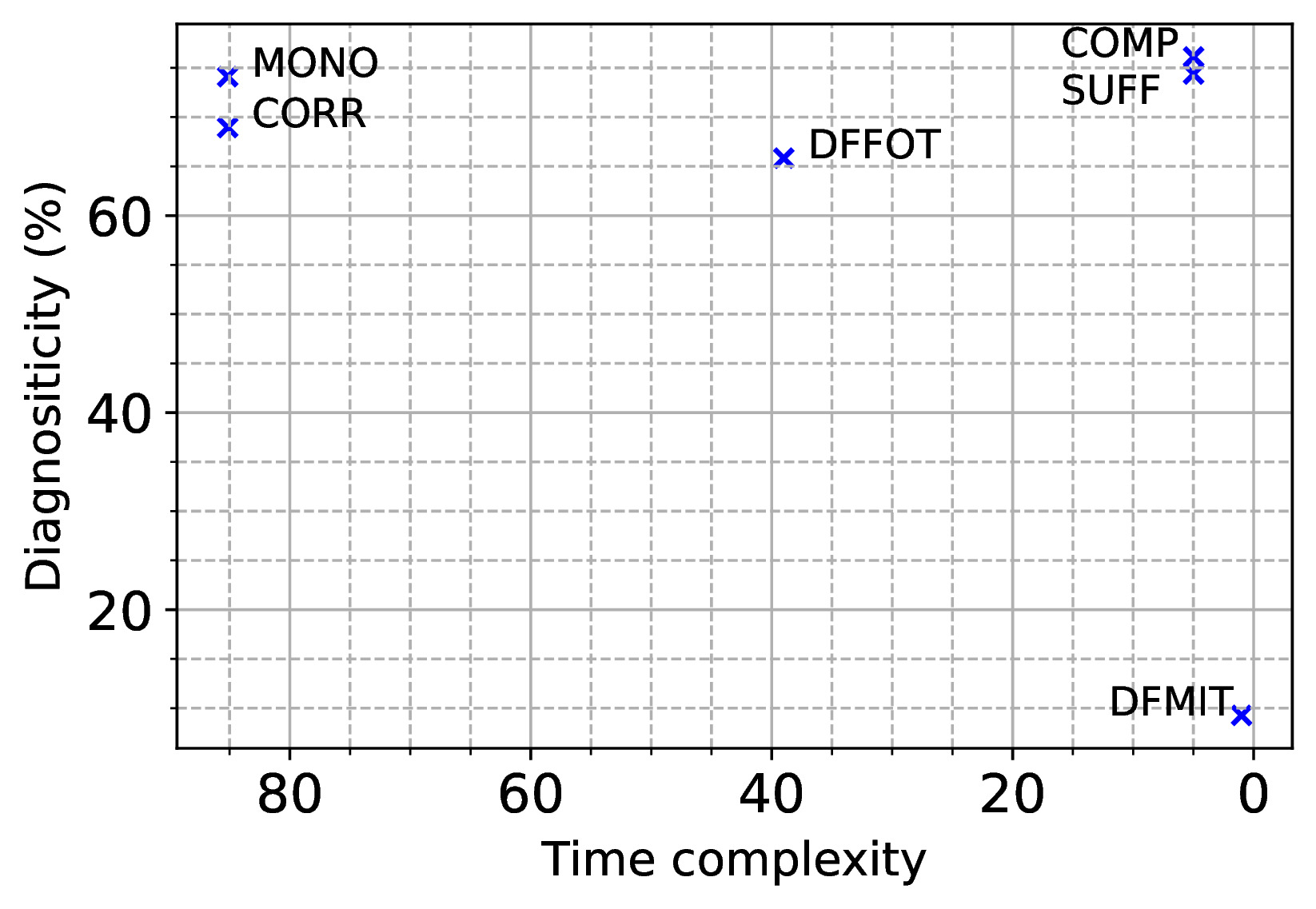
Figure 1: Diagnosticity vs time complexity for faithfulness metrics. The values are averages over all datasets and classification models. The faithfulness metrics near the top-right corner are more desirable than those near the bottom-left corner.

In Figure 1, we evaluate the faithfulness metrics by both their diagnosticities and time complexities.

Figure 1 suggests that we should always adopt COMP and SUFF. Because (i) they have higher diagnosticities and lower time complexities than DFFOT, ; (ii) they have a similar level of diagnosticity and much lower time complexities than CORR and MONO; (iii) DFMIT has diagnosticity less than 0.1, which is below an acceptable level. We would prefer COMP and SUFF over DFMIT even though it has the lowest time complexity.

Note that our evaluation framework can be used to compare any faithfulness metrics. In general, we prefer faithfulness metrics that have higher diagnosticities and lower time complexities, i.e. closer to the top-right corner in Figure 1. But what if one has a higher diagnosticity and the other one has a lower time complexity? In this case, we should consider diagnosticity first: a faithfulness metric should not be used if it cannot effectively assess faithfulness, i.e. diagnosticity below a certain threshold. In scenarios where we are subject to constraints of hardware or timeliness, we might need to select a faster metric with a lower but acceptable level of diagnosticity.

7 Related Work

Interpretation methods

Interpretation methods can be roughly classified into two categories: model-based methods and post-hoc methods. Model-based methods refer to the construction of simple machine learning models whose internal decision logic can be easily interpreted, such as linear regression models, decision trees, etc. Post-hoc methods interpret the internal reasoning process behind the model after training. Generally, post-hoc methods can be divided into gradient-based and perturbation-based. A gradient-based interpretation method assumes deep learning model is differentiable and discloses the decision making mechanism of the model according to the gradient information Simonyan et al. (2014); Sundararajan et al. (2017); Shrikumar et al. (2019). A perturbation-based interpretation method interprets the model by perturbing the input of data samples and measuring how the predictions change Robnik-Šikonja and Kononenko (2008); Zeiler and Fergus (2013); Ribeiro et al. (2016).

Interpretation method evaluation

To assess the quality of different interpretation methods, various evaluation metrics have been proposed. Existing evaluation methods on interpretations can be broadly classified into two categories, plausibility and faithfulness. Plausibility measures if the interpretation agrees with human judgments on how a model makes a decision Ribeiro et al. (2016); Doshi-Velez and Kim (2017); Lundberg and Lee (2017); DeYoung et al. (2020). However, even if the interpretation conforms to human criteria, it is not certain that it truly reflects the underlying decision mechanism behind the model. To this end, faithfulness measures the extent to which the inner decision-making mechanism actually relies on the identified important features Arras et al. (2017); Serrano and Smith (2019); Jain and Wallace (2019); Wiegreffe and Pinter (2019); DeYoung et al. (2020); Chrysostomou and Aletras (2021).

In general, existing faithfulness metrics are developed through a removal-based criterion, which measures the changes in model output when perturbing or removing tokens identified as important by the interpretation. Serrano and Smith (2019) proposed a decision flipping metric that evaluates the proportion of tokens that need to be erased in order to change the model decision. Also using decision flip as an indicator, Chrysostomou and Aletras (2021) introduces a metric that counts the average flips that occur when removing the most important token marked by the interpretation method. In addition to decision flips, changes in model output probabilities by removing or retaining important tokens is also widely used to measure faithfulness Arras et al. (2017); Arya et al. (2019); DeYoung et al. (2020).

Some recent work also focuses on the study of faithfulness metrics. Jacovi and Goldberg (2020) argued that the definition of faithfulness remains inconsistent and informal, and provided concrete guidelines on how evaluations of interpretation methods should and should not be conducted. More recently, Yin et al. (2021) discussed the limitations of removal-based faithfulness metrics and proposed two other quantitative criteria, namely sensitivity and stability. Different from the aforementioned previous work that does not focus on assessing faithfulness metrics, we mainly focus on the measurement of faithfulness and conduct a comprehensive study of existing faithfulness metrics.

8 Conclusion

In this paper, we propose a framework to quantitatively evaluate six widely adopted faithfulness metrics in terms of diagnosticity and time complexity. In particular, diagnosticity measures whether the faithfulness metric correctly favours relatively faithful interpretations over random ones; time complexity is concerned with computational efficiency, estimated by the average number of model forward passes. The experimental results show that sufficiency and comprehensiveness metrics outperform the other faithfulness metrics with higher diagnosticity and lower time complexity. For this reason, we suggest using these two metrics for faithfulness evaluation. We hope our work will bring more awareness to the standardization of faithfulness measurement. For future work, we would like to explore evaluating faithfulness metrics using a white-box model such as linear regression, from which we can derive an intrinsically faithful interpretation as the “ground truth”.

Appendix A Proof of Theorem 4.1

Proof.

Let $(u,v)$ be an interpretation pair. Then

$$\begin{split}&\text{P}(u\succ_{F}v|\text{P}(u\succ v)=1-\varepsilon)\\ &=\text{P}(u\succ_{F}v|u\succ v)(1-\varepsilon)+\text{P}(u\succ_{F}v|u\nsucc v)\varepsilon\\ &=\text{D}(F)+[\text{P}(u\succ_{F}v|u\nsucc v)-\text{P}(u\succ_{F}v|u\succ v)]\varepsilon\end{split}$$

Since $-1\leq\text{P}(u\succ_{F}v|u\nsucc v)-\text{P}(u\succ_{F}v|u\succ v)\leq 1$, we have

$$|\text{P}(u\succ_{F}v|\text{P}(u\succ v)=1-\varepsilon)-\text{D}(F)|\leq\varepsilon$$

∎

Appendix B Proof of Lemma 4.2

Proof.

From Definition 4.2, we have $\mathbbm{1}(u\succ_{F}v)|(\text{P}(u\succ v)>1-\varepsilon)\sim\text{Bernoulli}(p)$, where $p=\text{D}(F)$. Then based on the property of Bernoulli distribution, we know that the expected value of the random variable is equal to $p$. ∎

Appendix C Implementation Details

C.1 Text classification models

The text classification models are all implemented in PyTorch . For BERT, we use the “bert-base-uncased” from Huggingface transformers as the pretrained model . We use the same set of hyperparameters regardless of dataset for fine-tuning: dropout rate 0.2, AdamW Loshchilov and Hutter (2019) with an initial learning rate 2e-5, batch size 32 with no warmup steps. We set the maximum number of finetuning epochs to be 10 and perform early stopping when the performance on the test set does not improve for 3 consecutive epochs

For CNN classifier, we use a one-layer CNN encoder with a linear classifier. The embedding is initialized with the 300-dimensional pretrained GloVe word embedding Pennington et al. (2014). The CNN layer has 256 kernels and the size of the kernels is 3. We use max-pooling and AdamW with an initial learning rate 1e-3, batch size 32, with no warmup steps. The maximum number of epochs is 40 with early stopping after 3 consecutive non-improving epochs.

C.2 Interpretation methods

For LIME, Saliency Map, Integrated Gradients and DeepLift, we apply the implementation in Captum . For Word Omission, we use our own implementation.

References

- Alvarez-Melis and Jaakkola (2018) David Alvarez-Melis and Tommi S. Jaakkola. 2018. On the robustness of interpretability methods. Cite arxiv:1806.08049Comment: presented at 2018 ICML Workshop on Human Interpretability in Machine Learning (WHI 2018), Stockholm, Sweden.
- Arras et al. (2017) Leila Arras, Franziska Horn, Grégoire Montavon, Klaus-Robert Müller, and Wojciech Samek. 2017. "what is relevant in a text document?": An interpretable machine learning approach. PLoS ONE, 12:E0181142.
- Arya et al. (2019) Vijay Arya, Rachel K. E. Bellamy, Pin-Yu Chen, Amit Dhurandhar, Michael Hind, Samuel C. Hoffman, Stephanie Houde, Q. Vera Liao, Ronny Luss, Aleksandra Mojsilović, Sami Mourad, Pablo Pedemonte, Ramya Raghavendra, John Richards, Prasanna Sattigeri, Karthikeyan Shanmugam, Moninder Singh, Kush R. Varshney, Dennis Wei, and Yunfeng Zhang. 2019. One explanation does not fit all: A toolkit and taxonomy of ai explainability techniques.
- Brown et al. (2020) Tom B. Brown, Benjamin Mann, Nick Ryder, Melanie Subbiah, Jared Kaplan, Prafulla Dhariwal, Arvind Neelakantan, Pranav Shyam, Girish Sastry, Amanda Askell, Sandhini Agarwal, Ariel Herbert-Voss, Gretchen Krueger, Tom Henighan, Rewon Child, Aditya Ramesh, Daniel M. Ziegler, Jeffrey Wu, Clemens Winter, Christopher Hesse, Mark Chen, Eric Sigler, Mateusz Litwin, Scott Gray, Benjamin Chess, Jack Clark, Christopher Berner, Sam McCandlish, Alec Radford, Ilya Sutskever, and Dario Amodei. 2020. Language models are few-shot learners.
- Chrysostomou and Aletras (2021) George Chrysostomou and Nikolaos Aletras. 2021. Improving the faithfulness of attention-based explanations with task-specific information for text classification. In Proceedings of the 59th Annual Meeting of the Association for Computational Linguistics and the 11th International Joint Conference on Natural Language Processing (Volume 1: Long Papers), pages 477–488, Online. Association for Computational Linguistics.
- Devlin et al. (2019a) Jacob Devlin, Ming-Wei Chang, Kenton Lee, and Kristina Toutanova. 2019a. Bert: Pre-training of deep bidirectional transformers for language understanding.
- Devlin et al. (2019b) Jacob Devlin, Ming-Wei Chang, Kenton Lee, and Kristina Toutanova. 2019b. BERT: Pre-training of deep bidirectional transformers for language understanding. In Proceedings of the 2019 Conference of the North American Chapter of the Association for Computational Linguistics: Human Language Technologies, Volume 1 (Long and Short Papers), pages 4171–4186, Minneapolis, Minnesota. Association for Computational Linguistics.
- DeYoung et al. (2020) Jay DeYoung, Sarthak Jain, Nazneen Fatema Rajani, Eric Lehman, Caiming Xiong, Richard Socher, and Byron C. Wallace. 2020. ERASER: A benchmark to evaluate rationalized NLP models. In Proceedings of the 58th Annual Meeting of the Association for Computational Linguistics, pages 4443–4458, Online. Association for Computational Linguistics.
- Doshi-Velez and Kim (2017) Finale Doshi-Velez and Been Kim. 2017. Towards a rigorous science of interpretable machine learning.
- Jacovi and Goldberg (2020) Alon Jacovi and Yoav Goldberg. 2020. Towards faithfully interpretable NLP systems: How should we define and evaluate faithfulness? In Proceedings of the 58th Annual Meeting of the Association for Computational Linguistics, pages 4198–4205, Online. Association for Computational Linguistics.
- Jain and Wallace (2019) Sarthak Jain and Byron C. Wallace. 2019. Attention is not Explanation. In Proceedings of the 2019 Conference of the North American Chapter of the Association for Computational Linguistics: Human Language Technologies, Volume 1 (Long and Short Papers), pages 3543–3556, Minneapolis, Minnesota. Association for Computational Linguistics.
- Kim (2014) Yoon Kim. 2014. Convolutional neural networks for sentence classification. In Proceedings of the 2014 Conference on Empirical Methods in Natural Language Processing (EMNLP), pages 1746–1751, Doha, Qatar. Association for Computational Linguistics.
- Liu et al. (2019) Yinhan Liu, Myle Ott, Naman Goyal, Jingfei Du, Mandar Joshi, Danqi Chen, Omer Levy, Mike Lewis, Luke Zettlemoyer, and Veselin Stoyanov. 2019. Roberta: A robustly optimized bert pretraining approach.
- Loshchilov and Hutter (2019) Ilya Loshchilov and Frank Hutter. 2019. Decoupled weight decay regularization.
- Lundberg and Lee (2017) Scott Lundberg and Su-In Lee. 2017. A unified approach to interpreting model predictions.
- Maas et al. (2011) Andrew L. Maas, Raymond E. Daly, Peter T. Pham, Dan Huang, Andrew Y. Ng, and Christopher Potts. 2011. Learning word vectors for sentiment analysis. In Proceedings of the 49th Annual Meeting of the Association for Computational Linguistics: Human Language Technologies, pages 142–150, Portland, Oregon, USA. Association for Computational Linguistics.
- Pennington et al. (2014) Jeffrey Pennington, Richard Socher, and Christopher Manning. 2014. GloVe: Global vectors for word representation. In Proceedings of the 2014 Conference on Empirical Methods in Natural Language Processing (EMNLP), pages 1532–1543, Doha, Qatar. Association for Computational Linguistics.
- Ribeiro et al. (2016) Marco Ribeiro, Sameer Singh, and Carlos Guestrin. 2016. “why should I trust you?”: Explaining the predictions of any classifier. In Proceedings of the 2016 Conference of the North American Chapter of the Association for Computational Linguistics: Demonstrations, pages 97–101, San Diego, California. Association for Computational Linguistics.
- Robnik-Šikonja and Kononenko (2008) Marko Robnik-Šikonja and Igor Kononenko. 2008. Explaining classifications for individual instances. IEEE Transactions on Knowledge and Data Engineering, 20(5):589–600.
- Serrano and Smith (2019) Sofia Serrano and Noah A. Smith. 2019. Is attention interpretable? In Proceedings of the 57th Annual Meeting of the Association for Computational Linguistics, pages 2931–2951, Florence, Italy. Association for Computational Linguistics.
- Shrikumar et al. (2019) Avanti Shrikumar, Peyton Greenside, and Anshul Kundaje. 2019. Learning important features through propagating activation differences.
- Simonyan et al. (2014) Karen Simonyan, Andrea Vedaldi, and Andrew Zisserman. 2014. Deep inside convolutional networks: Visualising image classification models and saliency maps.
- Socher et al. (2013) Richard Socher, Alex Perelygin, Jean Wu, Jason Chuang, Christopher D. Manning, Andrew Ng, and Christopher Potts. 2013. Recursive deep models for semantic compositionality over a sentiment treebank. In Proceedings of the 2013 Conference on Empirical Methods in Natural Language Processing, pages 1631–1642, Seattle, Washington, USA. Association for Computational Linguistics.
- Sundararajan et al. (2017) Mukund Sundararajan, Ankur Taly, and Qiqi Yan. 2017. Axiomatic attribution for deep networks. In Proceedings of the 34th International Conference on Machine Learning - Volume 70, ICML’17, page 3319–3328. JMLR.org.
- Vaswani et al. (2017) Ashish Vaswani, Noam Shazeer, Niki Parmar, Jakob Uszkoreit, Llion Jones, Aidan N Gomez, Ł ukasz Kaiser, and Illia Polosukhin. 2017. Attention is all you need. In Advances in Neural Information Processing Systems, volume 30. Curran Associates, Inc.
- Wiegreffe and Pinter (2019) Sarah Wiegreffe and Yuval Pinter. 2019. Attention is not not explanation. In Proceedings of the 2019 Conference on Empirical Methods in Natural Language Processing and the 9th International Joint Conference on Natural Language Processing (EMNLP-IJCNLP), pages 11–20, Hong Kong, China. Association for Computational Linguistics.
- Yin et al. (2021) Fan Yin, Zhouxing Shi, Cho-Jui Hsieh, and Kai-Wei Chang. 2021. On the faithfulness measurements for model interpretations.
- Zeiler and Fergus (2013) Matthew D Zeiler and Rob Fergus. 2013. Visualizing and understanding convolutional networks.
- Zhang et al. (2015) Xiang Zhang, Junbo Zhao, and Yann LeCun. 2015. Character-level convolutional networks for text classification. In Proceedings of the 28th International Conference on Neural Information Processing Systems - Volume 1, NIPS’15, page 649–657, Cambridge, MA, USA. MIT Press.