Lie Symmetries, Painlevé analysis and global dynamics for the temporal equation of radiating stars

Abstract

[Abstract]We study the temporal equation of radiating stars by using three powerful methods for the analysis of nonlinear differential equations. Specifically, we investigate the global dynamics for the given master ordinary differential equation to understand the evolution of solutions for various initial conditions as also to investigate the existence of asymptotic solutions. Moreover, with the application of Lie’s theory, we can reduce the order of the master differential equation, while an exact similarity solution is determined. Finally, the master equation possesses the Painlevé property, which means that the analytic solution can be expressed in terms of a Laurent expansion.

10.1002/mma.8274

Leon G, Govender M, Paliathanasis A. Lie symmetries, Painlevé analysis, and global dynamics for the temporal equation of radiating stars. Math Meth Appl Sci. 2022;1-16. doi:10.1002/mma.8274

1 Introduction

Ordinary differential equations play an important role in the study of physical systems. There are various approaches for the study of the properties of physical systems described by differential equations as well as to construct and determine exact and analytic solutions. Relativistic astrophysics is an active area employing various solution-generating techniques to solve highly nonlinear systems of differential equations. From finding exact solutions of the Einstein field equations or their modifications (Einstein-Gauss Bonnet gravity, $f(R)$ gravity or Brans-Dicke theory, etc.) describing stellar objects through to the study of causal thermodynamics, where solutions of governing differential equations have played a key role.

The end-states of gravitational collapse of bounded configurations have held the attention of astrophysicists since the pioneering work of Oppenheimer and Snyder¹ in which they studied idealised collapse of a dust sphere. The Weak Cosmic Censorship Conjecture, first articulated by Penrose, forbids the existence of naked singularities arising from continued gravitational collapse. However, there have been many counter-examples put forward within the framework of Einstein’s classical general relativity ^{2, 3, 4, 5}. The confirmation of classical general relativity as a cornerstone of gravitational theory was borne out in 2019 when the photograph of the shadow of a black hole ⁶ was obtained, heralding a new frontier of theoretical predictions and observations. The discovery of the Vaidya solution ⁷ paved the way for researchers to study dissipative collapse of stars. The boundary of the collapsing object divides spacetime into two distinct regions, ${\cal M^{-}}$, the interior region and ${\cal M^{+}}$, the exterior region described by the Vaidya solution. Early work on dissipative gravitational collapse can be attributed to Herrera and co-workers (see ^{8, 9} and references therein). In their investigations they studied spherically symmetric, shear-free stellar objects undergoing dissipative gravitational collapse in the form of a radial heat flux. The junction conditions for the smooth matching of the interior spacetime to the exterior Vaidya solution were derived by Santos ¹⁰. The Santos junction conditions demonstrated that the pressure at the boundary of a collapsing, radiating star is nonzero and is proportional to the magnitude of the outgoing radial heat flux. This junction condition represents the conservation of momentum across the boundary of the collapsing star. Recently, the Santos junction conditions have been extended to include a dynamically unstable core with a general energy-momentum tensor describing an imperfect fluid with heat flux and null radiation with the exterior being described by the generalised Vaidya solution ¹¹. Over the next two decades, the study of radiating stars has provided us with a rich insight into the end-states of continued gravitational collapse, particularly with regards to time of formation of the horizon¹², temperature profiles and relaxational effects related to causal heat flux¹³. The shear-free models were subsequently extended to include the effects of shear viscosity. It has been demonstrated that the Chandrasekhar stability criterion for isotropic fluid spheres is modified in the presence of shear viscosity. Furthermore, in both the Newtonian and relativistic regimes, the shear viscosity decreases the instability of the stellar fluid¹⁴.

The inclusion of shear, anisotropy, electromagnetic field, and rotation in the slow approximation have been fruitful in studying the thermodynamics of such systems. The impact of shear on the kinematics and dynamics of the collapse process has been addressed by several authors. The instability of the shear-free condition has been demonstrated by Herrera et al. ¹⁵ in which they showed that the shear-free condition may hold for a limited epoch of the collapse process. The presence of pressure anisotropies, density inhomogeneities, and dissipative fluxes can mimic shear-like effects ¹⁶. The inclusion of shear during dissipative collapse has led to interesting results when contrasted to the shear-free case. Shearing effects lead to higher core temperatures it has been shown that horizon formation is delayed when shear is present. In an attempt to model shearing, radiating stars, Ivanov introduced the so-called horizon function which simplifies the boundary condition representing the temporal behavior of the model^{17, 18}. The horizon function has a physical attribute in the sense that it is directly related to the surface redshift of the collapsing sphere. Once this function is determined from the boundary condition, the end-state or possible outcome of continued gravitational collapse can be studied. The avoidance of the singularity was demonstrated by using a simple model of shear-free collapse in which the rate of collapse is balanced by the rate of energy emission to the exterior spacetime ¹⁹. This so-called horizon-free model, or Banerjee, Chatterjee & Dadhich (BCD) ¹⁹ model, forms the basis of the work contained in this paper. The horizon-free collapse in the presence of shear was studied in various models in which the gravitational potentials were highly simplified. The so-called Euclidean stars, in which the areal radius is equal to the proper radius were shown to undergo horizon-free collapse ²⁰. The BCD model has two inherent assumptions: the interior spacetime is shear-free and the gravitational potentials are separable in space and time. Works by Chan and co-workers attempted to generalise the shear-free model to include shear by demanding that the metric functions be separable. These models have several drawbacks such as the proper radius being independent of time or the resulting boundary condition rendered solvable via numerical methods^{21, 22}.

In this piece of work, we investigate the dynamics for the master equation of the temporal equation of radiating stars. The equation that we are interested describes the Einstein field equations for a spherically symmetric line element

$$ds^{2}=-A^{2}(r,t)dt^{2}+B^{2}(r,t)\left(dr^{2}+r^{2}d\theta^{2}+r^{2}\sin^{2}\theta d\phi^{2}\right),$$ (1)

for a pressure isotropy fluid with an exterior solution the Vaidya metric ⁷ such that to describe a radiative solution. Banerjee et al. ²³ suggested the metric ansatz $A\left(t,r\right)=1+\zeta_{0}r^{2},~{}B\left(t,r\right)=R(t)~{}$where $\zeta_{0}$ is a positive constant. In this case, the field equations reduce to the second-order differential equation

$$2R(t){\ddot{R}}(t)+{\dot{R}(t)}^{2}+\alpha{\dot{R}(t)}=\beta,$$ (2)

where $\alpha$ and $\beta$ are constants and the dot means derivative with respect to the time $t$. A special solution of the latter equation is the solution $R=-Ct$ where $C>0$ is a constant, which describes a collapsing star ²³. Recently, in ²⁴ new families of exact solutions for the master equation (2) were found using Lie symmetries. This body of work forms part of several investigations about dissipative collapse via Lie symmetries. Radiating stars with shear, in which the particle trajectories within the stellar fluid were geodesics, were studied using Lie symmetries²⁵. Several new solutions were obtained while other solutions were reduced to well-known cases studied earlier in the literature. The geodesic case with shear was extended to the most general shearing matter distribution radiating energy to the exterior spacetime. The method of Lie symmetries proved useful in obtaining four new classes of solutions ²⁶, two of which included the horizon function and the Euclidean condition.

In the following, we study the dynamics and the stability properties for the master equation (2) and also, we show in detail how the method of Lie point symmetries and the singularity analysis can be used for the derivation of new analytic and exact solution for equation (2).

The theory of Lie symmetries ²⁷ is a powerful approach for the investigation of invariant functions for differential equations. The novelty of Lie theory is that the infinitesimal representations of the finite transformations of continuous groups are considered, by moving from the group to a local algebraic representation, and to studying the invariance properties under them. The resulting invariant functions can be used for the reduction of order for a given ordinary differential equation and consequently for the derivation of solutions. These exact solutions which follow from the application of Lie symmetries are known as similarity solutions. The theory of Lie symmetries cover a range of applications in physical science and gravitational theory, see for instance ^{28, 29, 30, 31, 32, 33} and references therein.

The singularity analysis, which is mainly associated with the school of Painlevé, that is why also it is called Painlevé analysis ³⁴, is another powerful mathematical approach for the derivation of solutions of differential equations. When a differential equation passes the singularity the analysis we say that the differential equation possesses the Painlevé property. Nowadays the application of the singularity analysis is summarised in ARS algorithm, from the initials of Ablowitz, Ramani, and Segur ^{35, 36, 37} who established a systematic method for investigation of analytic solutions, inspired by the approach applied by Kowalevskaya ³⁸ for the determination of the third integrable case of Euler’s equations for a spinning top. The basic characteristic for a differential equation to possesses the Painlevé property is the existence of at least a movable singularity. In the singularity analysis the analytic solution for a given differential equation is expressed by Painlevé Series, and specifically in our consideration we shall write the analytic solution in the Puiseux series.

On the other hand, stability analysis provides us with an important tool to investigate the evolution of the given dynamical system. Indeed, from the stability analysis, we can investigate if a given solution is stable or not, while we can determine families of initial conditions such that specific behavior for the dynamical system to be stable. In addition, we can define constraints for the free parameters of the differential equations according to the stability of exact solutions. Hence, we can extract important information about the nature of the free parameters. In our consideration, for equation (2)  we can understand how the free parameters $\alpha$ and $\beta$ affects the dynamics. The plan of the paper is as follows.

In Section 2 we investigate the stability properties for the master equation (2) for the exact solution found in ²³, while we perform a detailed study of the global dynamics for the master equation. From the dynamical analysis, a new family of exact solutions is constructed. In Section 3, we investigate equation (2) by applying Lie’s theory, as we study if equation (2) possesses the Painlevé property. We find that the differential equation admits two Lie point symmetries which form the $A_{2,2}$ Lie algebra. Consequently, the application of the Lie symmetries provides two similarity transformations. Moreover, the application of the ARS algorithm indicates that the master equation (2) satisfies the Painlevé test, and the analytic solution is expressed by a right Painlevé series. However, for a specific relation between the two free variables $\alpha$, $\beta$; a new exact solution is determined. Finally, in Section 4 we discuss our results and draw our conclusions.

2 Stability analysis and global dynamics

For the master equation (2),  by convenience we assume $\alpha>0$. A special and simple solution to this equation is $R=-Ct$ defined for $-\infty<t\leq 0$, where $C>0$ is a constant given by the positive roots of

$$-\beta+C^{2}-\alpha C=0.$$ (3)

That is, for $\beta>0$, we have only one positive root $C=\frac{1}{2}\left(\sqrt{\alpha^{2}+4\beta}+\alpha\right)$. For $\beta<0$ and $\alpha^{2}+4\beta>0$, we have two different positive roots: $C_{-}=\frac{1}{2}\left(\alpha-\sqrt{\alpha^{2}+4\beta}\right)$ and $\quad C_{+}=\frac{1}{2}\left(\sqrt{\alpha^{2}+4\beta}+\alpha\right)$.

To avoid ambiguities we prefer to use the relation $\beta=C^{2}-C\alpha$, and in the analysis separate the cases $\beta<0$ and $\beta\geq 0$.

For the analysis of stability of the scaling solution $R(t)=-Ct$, with $C=\frac{1}{2}\left(\sqrt{\alpha^{2}+4\beta}+\alpha\right)>0$ in the interval $-\infty<t<0$ we use similar methods as in Liddle & Scherrer ³⁹ and Uzan ⁴⁰. For this purpose, the new logarithmic time variable $\tau$ related to $t$ through

$$t=-e^{-\tau},\quad-\infty<\tau<\infty,$$ (4)

such that $t\rightarrow-\infty$ as $\tau\rightarrow-\infty$ and $t\rightarrow 0$ as $\tau\rightarrow+\infty$ is defined.

Then, replacing the relation between $t$ and $\tau$ given by (4) in the expression $R(t)$, we obtain a function of $\tau$ from $R(t)$ denoted and defined by

$$\bar{R}(\tau)=R(-e^{-\tau}).$$ (5)

Using again the transform (4), the scaling solution $R(t)=-Ct$ can be re-expressed as a function of $\tau$ as $R_{s}(\tau)=Ce^{-\tau}$.

To compare a generic solution $\bar{R}(\tau)$ with the scaling solution $R_{s}(\tau)=Ce^{-\tau}$, we define a dimensionless function of $\tau$ as the ratio

$$u(\tau)=\frac{\bar{R}(\tau)}{R_{s}(\tau)}.$$ (6)

Thus, the solution $R_{s}(\tau)$ will corresponds to the equilibrium point $u=1$ in the new formulation of the master equation (2). The physical region corresponds to $u\geq 0$. Recall, the physical solution $R=-Ct$ is defined for $-\infty<t\leq 0$, where $C>0$ is a constant.

To reformulate the master equation (2) in terms of $u(\tau)$, and its derivatives with respect to $\tau$, we use the chain rule to obtain several differentiation rules. Let be denoted the time derivative with respect to $\tau$ be denoted by a prime and the time derivative with respect to $t$ by a dot. That is, for $f(\tau)$, let

$$f^{\prime}(\tau)\equiv\frac{df(\tau)}{d\tau},$$ (7)

and for $g(t)$, let

$$\dot{g}(t)\equiv\frac{dg(t)}{dt}.$$ (8)

Then,

$$\dot{R}(t)=\frac{d\tau(t)}{dt}\bar{R}^{\prime}(\tau)=e^{\tau}\bar{R}^{\prime}(\tau),\quad\ddot{R}(t)=e^{2\tau}\left(\bar{R}^{\dprime}(\tau)+\bar{R}^{\prime}(\tau)\right)$$ (9)

and

$${R_{s}^{\prime}(\tau)}/{R_{s}(\tau)}=-1,\quad R_{s}(\tau)=Ce^{-\tau}.$$ (10)

Therefore, by using the rules (9), and substituting expression (4), the equation (2) becomes

$$-\beta+\alpha e^{\tau}\bar{R}^{\prime}(\tau)+e^{2\tau}\left({\bar{R}^{\prime}(\tau)}^{2}+2\bar{R}(\tau)\left(\bar{R}^{\dprime}(\tau)+\bar{R}^{\prime}(\tau)\right)\right)=0.$$ (11)

The next step is to rewrite equation (11) in terms of $u(\tau)$ and its derivatives.

Solving equation (6) for $\bar{R}$, and then using the derivatives rules for products of functions and the chain rule, we obtain, subsequently,

$$\bar{R}(\tau)=Ce^{-\tau}u(\tau),$$ (12)

$$\bar{R}^{\prime}(\tau)=Ce^{-\tau}\left(u^{\prime}(\tau)-u(\tau)\right),$$ (13)

$$\bar{R}^{\dprime}(\tau)=Ce^{-\tau}\left(u^{\dprime}(\tau)-2u^{\prime}(\tau)+u(\tau)\right).$$ (14)

Substituting (12), (13) and (14) in equation (11), and dividing by the overall factor $e^{-\tau}$, we obtain

$$2C^{2}u(\tau)u^{\dprime}(\tau)+C^{2}{u^{\prime}(\tau)}^{2}+Cu^{\prime}(\tau)(\alpha-4Cu(\tau))+C(u(\tau)-1)(-\alpha+Cu(\tau)+C)=0.$$ (15)

where we have used the relation $\beta=C^{2}-C\alpha$.

Defining the new function

$$v(\tau)=u^{\prime}(\tau),$$ (16)

we obtain the dynamical system

$$u^{\prime}(\tau)=v(\tau),$$ (17)

$$v^{\prime}(\tau)=-\frac{(u(\tau)-1)(-\alpha+Cu(\tau)+C)}{2Cu(\tau)}+v(\tau)\left(2-\frac{\alpha}{2Cu(\tau)}\right)-\frac{v(\tau)^{2}}{2u(\tau)}.$$ (18)

The scaling solution $R_{s}(\tau)=Ce^{-\tau}$ corresponds to the equilibrium point $u=1,v=0$.

Defining $\varepsilon$ through $u=1+\varepsilon$, we obtain the final dynamical system

$$\varepsilon^{\prime}(\tau)=v(\tau),$$ (19)

$$v^{\prime}(\tau)=\frac{\varepsilon(\tau)(\alpha-C\varepsilon(\tau)-2C)}{2C(\varepsilon(\tau)+1)}+v(\tau)\left(2-\frac{\alpha}{2C\varepsilon(\tau)+2C}\right)-\frac{v(\tau)^{2}}{2(\varepsilon(\tau)+1)},$$ (20)

where the equilibrium point is translated to the origin.

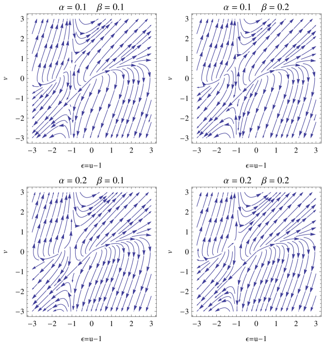
Figure 1: Phase plot of (17), (18) for some $\alpha>0,\beta>0$ and the choice $2C:=\alpha+\sqrt{\alpha^{2}+4\beta}$. The origin represents the solution $R_{s}(\tau)=Ce^{-\tau}$, which is unstable (node). The physical region corresponds to $u\geq 0$.

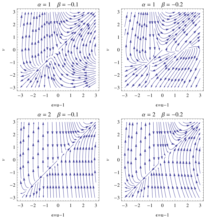
Figure 2: Phase plot of (17), (18) for some $\alpha>0,\beta<0$ and the choice $2C_{-}:=\alpha-\sqrt{\alpha^{2}-4|\beta|}$. The origin represents the solution $R_{s-}(\tau)=C_{-}e^{-\tau}$, which is unstable (saddle). The physical region corresponds to $u\geq 0$.

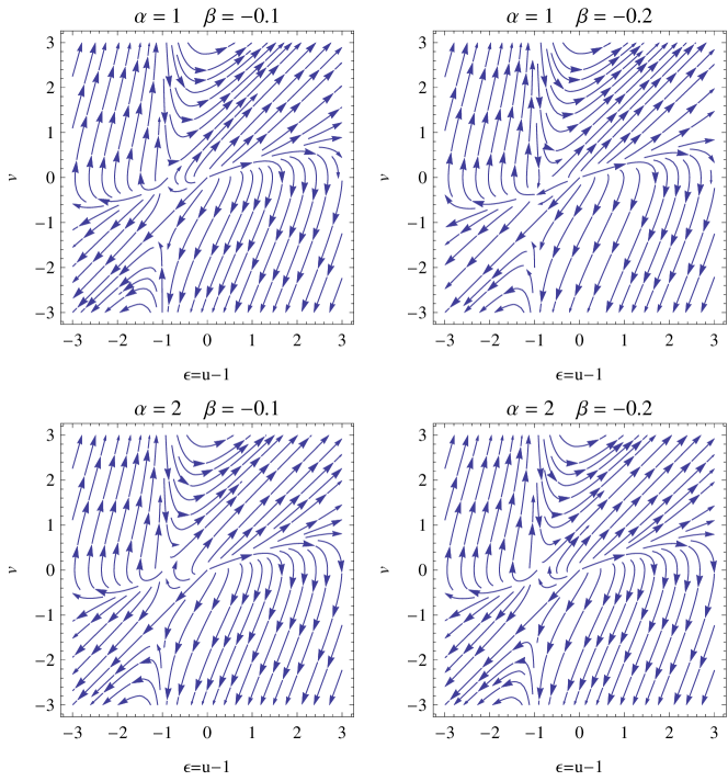
Figure 3: Phase plot of (17), (18) for some $\alpha>0,\beta<0$ and the choice $2C_{+}:=\alpha+\sqrt{\alpha^{2}-4|\beta|}$. The origin represents the solution $R_{s+}(\tau)=C_{+}e^{-\tau}$, which is unstable (node). The physical region corresponds to $u\geq 0$.

The linearisation matrix is defined by

$$J(\varepsilon,v)=\left(\begin{array}[c]{cc}0&1\\ \frac{1}{2}\left(\frac{(v+1)(vC-C+\alpha)}{C(\varepsilon+1)^{2}}-1\right)&2-\frac{\alpha+2Cv}{2\varepsilon C+2C}\end{array}\right).$$ (21)

Then, linearising around the equilibrium point, $\varepsilon=0,v=0$, we obtain

$$\left(\begin{array}[c]{c}\varepsilon^{\prime}(\tau)\\ v^{\prime}(\tau)\end{array}\right)=\left(\begin{array}[c]{cc}0&1\\ -1+\frac{\alpha}{2C}&2-\frac{\alpha}{2C}\end{array}\right)\left(\begin{array}[c]{c}\varepsilon(\tau)\\ v(\tau)\end{array}\right).$$ (22)

The linearisation matrix

$$J(0,0)=\left(\begin{array}[c]{cc}0&1\\ \frac{\alpha}{2C}-1&2-\frac{\alpha}{2C}\end{array}\right)$$ (23)

has eigenvalues $\left\{1,1-\frac{\alpha}{2C}\right\}$.

Assume first $\beta\geq 0$. In this case, the origin is always unstable as $\tau\rightarrow+\infty$ due to $2C=\alpha+\sqrt{\alpha^{2}+4\beta}>\alpha$. That is, the origin is stable as $\tau\rightarrow-\infty$.

An additional equilibrium point is

$$\varepsilon=\frac{\alpha}{C}-2<0,\quad u=\frac{\alpha}{C}-1,\quad v=0.$$ (24)

Evaluating the linearisation matrix $J\left(\frac{\alpha}{C}-2,0\right)$, we obtain the eigenvalues $\left\{1,\frac{2C-\alpha}{2(C-\alpha)}\right\}$. Due to $2C-\alpha>0$ it is unstable as $\tau\rightarrow\infty$. Indeed for $0<\frac{\alpha}{2}<C<\alpha$ it is a saddle, whereas for $C>\alpha>0$ is an unstable node. The last conditions is forbidden due to the physical condition $u\geq 0$ evaluated at $(u,v)=\left(\frac{\alpha}{C}-1,0\right)$ implies $\alpha\geq C$.

Now, let us study the case $\beta<0,\alpha<-2\sqrt{-\beta}$ or $\beta<0,\alpha>2\sqrt{-\beta}$. Henceforth, we have two solutions

$$R_{s\pm}(\tau)=-C_{\pm}t(\tau)=C_{\pm}e^{-\tau},$$ (25)

where

$$2C_{\pm}=\alpha\pm\sqrt{\alpha^{2}-4|\beta|}.$$ (26)

Observe that $2C_{+}>\alpha$, implies that $R_{s+}(\tau)$ is an unstable solution (unstable node) as $\tau\rightarrow\infty$. Due to $\alpha>2C_{-}>0$, $R_{s-}(\tau)$ is an unstable (saddle) solution.

Figure 1 shows the phase plot of system (17), (18) for some $\alpha>0,\beta>0$ and the choice $2C:=\alpha+\sqrt{\alpha^{2}+4\beta}$. The origin represents the solution $R_{s}(\tau)=Ce^{-\tau}$, which is unstable (node).

Figure 2 shows the phase plot of system (17), (18) for some $\alpha>0,\beta<0$ and the choice $2C_{-}:=\alpha-\sqrt{\alpha^{2}-4|\beta|}$. The origin represents the solution $R_{s-}(\tau)=C_{-}e^{-\tau}$, which is unstable (saddle).

Figure 3 shows the phase plot of system (17), (18) for some $\alpha>0,\beta<0,\alpha^{2}+4\beta\geq 0$ and the choice $2C_{+}:=\alpha+\sqrt{\alpha^{2}-4|\beta|}$. The origin represents the solution $R_{s+}(\tau)=C_{+}e^{-\tau}$, which is unstable (node).

As can be seen in figures 1, 2 and 3, there are non-trivial dynamics as $(u,v)$ are unbounded.

2.1 Dynamics as $(u,v)$ are unbounded

Assume that there are $u_{0}>0$, and a coordinate transformation $\phi=h(u)$, with inverse $h^{(-1)}(\phi)$, which maps the interval $[u_{0},\infty)$ onto $(0,\delta]$, where $\delta=h(u_{0})$, satisfying $\lim_{u\rightarrow+\infty}h(u)=0$, and has the following additional properties:

1. $h$ is $C^{k+1}$ and strictly decreasing,

2. $$\overline{h^{\prime}}(\phi)=\left\{\begin{array}[c]{cc}h^{\prime}(h^{(-1)}(\phi)),&\phi>0,\\ \lim_{\phi\rightarrow\infty}h^{\prime}(\phi),&\phi=0\end{array}\right.$$ (27)

   is $C^{k}$ on the closed interval $[0,\delta]$ and

3. $\frac{d\overline{h^{\prime}}}{d\phi}(0)$ and higher derivatives $\frac{d^{m}\overline{h^{\prime}}}{d\phi^{m}}(0)$ satisfy

   $$\frac{d\overline{h^{\prime}}}{d\phi}(0)=\frac{d^{m}\overline{h^{\prime}}}{d\phi^{m}}(0)=0.$$ (28)

It can be proved using the above conditions that

$$\lim_{\phi\rightarrow 0}\frac{1}{h^{(-1)}(\phi)}=0,$$ (29)

$$\lim_{\phi\rightarrow 0}\frac{h^{\prime}\left(h^{(-1)}(\phi)\right)}{\phi}=0,$$ (30)

$$\lim_{\phi\rightarrow 0}\quad\frac{h^{\prime\prime}\left(h^{(-1)}(\phi)\right)}{h^{\prime}\left(h^{(-1)}(\phi)\right)}=0.$$ (31)

In the following, we say that $g$ is well-behaved at infinity (WBI) of exponential order $N$, if there is $N$ such that

$$\lim_{u\rightarrow\infty}\left(\frac{g^{\prime}(u)}{g(u)}-N\right)=0.$$ (32)

Let $g$ be a WBI function of exponential order $N$ then, exponential dominated means, for all $\lambda>N$,

$$\lim_{u\to\infty}\,e^{-\lambda u}g(u)=0.$$ (33)

From

$$\lim_{\phi\to 0}\,\frac{h^{\prime\prime}\left(h^{(-1)}(\phi)\right)}{h^{\prime}\left(h^{(-1)}(\phi)\right)}=0,$$ (34)

it follows that $g(u)=1/h^{\prime}(u)$ is WBI of exponential order $0$, that is, $\lim_{u\rightarrow\infty}\frac{g^{\prime}(u)}{g(u)}-N=0$ for $N=0$, and hence it is exponential dominated. This implies in turn that $1/h(u)$ is also exponential dominated. The function $h(u)$ must therefore obey the following condition: for all $k>0$,

$$\lim_{u\rightarrow\infty}\frac{e^{ku}}{h^{\prime}\left(u\right)}=\lim_{u\rightarrow\infty}\frac{e^{ku}}{h(u)}=0.$$ (35)

In general, we can obtain functions $\phi=h(u)$ satisfying the above conditions 1, 2, 3, and previously commented facts if we demand the existence of $n>1$ such that the functions

$$\frac{1}{h^{(-1)}(\phi)},\quad\frac{h^{\prime}\left(h^{(-1)}(\phi)\right)}{\phi},\quad\frac{h^{\prime\prime}\left(h^{(-1)}(\phi)\right)}{h^{\prime}\left(h^{(-1)}(\phi)\right)},$$ (36)

behaves as $\mathcal{O}(\phi^{n})$, and

$$h^{(m)}\left(h^{(-1)}(\phi)\right)\sim\mathcal{O}(\phi^{(mn+1)}),\quad m\in\mathbb{N},\quad m\geq 1,$$ (37)

as $\phi\rightarrow 0$, where the superscript $(m)$ means $m$-th derivative with respect the argument.

Let be defined

$$\theta=1-u+v.$$ (38)

Then we obtain

$$\phi^{\prime}=\overline{h^{\prime}}(\phi)\left(h^{(-1)}(\phi)+\theta-1\right),$$ (39)

$$\theta^{\prime}=\frac{(2C-\alpha)\theta}{2Ch^{(-1)}(\phi)}-\frac{\theta^{2}}{2h^{(-1)}(\phi)},$$ (40)

where $\overline{h^{\prime}}(\phi)$ is defined in (27) and $2C-\alpha>0$. The system (39), (40) defines a flow in the phase region

$$\Omega_{\delta}:=\left\{(\phi,\theta)\in\mathbb{R}^{2}:0<\phi<h(\delta^{-1}),\theta\in K\right\},$$ (41)

where $K$ is a compact set, such that $\Omega_{\delta}$ is a positive invariant set for large $\tau$.

The system (39), (40) admits a curve of equilibrium points $L:(\phi,\theta)=(0,\theta^{*})$   parametrised by $\theta^{*}$ that is approached as $\tau\rightarrow\infty$ (for bounded $\theta$). This curve of equilibrium points is represented by a red dashed line in figures 4, 5 and 6.

The linearisation matrix of system (39) and (40) at a generic point $(\phi,\theta)$ is

$$J(\phi,\theta) =\left(\begin{array}[c]{cc}1+\frac{\left(\theta+h^{(-1)}(\phi)-1\right)h^{\prime\prime}\left(h^{(-1)}(\phi)\right)}{h^{\prime}\left(h^{(-1)}(\phi)\right)}&h^{\prime}\left(h^{(-1)}(\phi)\right)\\ \frac{(\alpha+C(\theta-2))\theta}{2Ch^{(-1)}(\phi)^{2}h^{\prime}\left(h^{(-1)}(\phi)\right)}&-\frac{\alpha+2C(\theta-1)}{2Ch^{(-1)}(\phi)}\\ &\end{array}\right)$$ (45)

$$=\left(\begin{array}[c]{cc}1+\frac{h^{(-1)}(\phi)h^{\prime\prime}\left(h^{(-1)}(\phi)\right)}{h^{\prime}\left(h^{(-1)}(\phi)\right)}+\mathcal{O}(\phi^{n})&h^{\prime}\left(h^{(-1)}(\phi)\right)\\ \frac{(\alpha+C(\theta-2))\theta}{2Ch^{(-1)}(\phi)^{2}h^{\prime}\left(h^{(-1)}(\phi)\right)}&\mathcal{O}(\phi^{n})\\ &\end{array}\right)$$ (49)

$$=\left(\begin{array}[c]{cc}1+\frac{h^{(-1)}(\phi)h^{\prime\prime}\left(h^{(-1)}(\phi)\right)}{h^{\prime}\left(h^{(-1)}(\phi)\right)}+\mathcal{O}(\phi^{n})&\mathcal{O}(\phi^{n+1})\\ \mathcal{O}(\phi^{n-1})&\mathcal{O}(\phi^{n})\\ &\end{array}\right)$$ (53)

$$\sim\left(\begin{array}[c]{cc}1+\frac{h^{(-1)}(\phi)h^{\prime\prime}\left(h^{(-1)}(\phi)\right)}{h^{\prime}\left(h^{(-1)}(\phi)\right)}&0\\ 0&0\\ &\end{array}\right),\quad\text{as}\;\phi\rightarrow 0,$$ (57)

We have,

$$J(\phi,\theta)$$

$$=\left(\begin{array}[c]{cc}1+\frac{h^{(-1)}(\phi)h^{\prime\prime}\left(h^{(-1)}(\phi)\right)}{h^{\prime}\left(h^{(-1)}(\phi)\right)}+\mathcal{O}(\phi^{n})&h^{\prime}\left(h^{(-1)}(\phi)\right)\\ \frac{(\alpha+C(\theta-2))\theta}{2Ch^{(-1)}(\phi)^{2}h^{\prime}\left(h^{(-1)}(\phi)\right)}&\mathcal{O}(\phi^{n})\\ &\end{array}\right)$$ (61)

has characteristic polynomial

$$\left(1+\frac{h^{(-1)}(\phi)h^{\prime\prime}\left(h^{(-1)}(\phi)\right)}{h^{\prime}\left(h^{(-1)}(\phi)\right)}-\lambda+\mathcal{O}(\phi^{n})\right)(-\lambda+\mathcal{O}(\phi^{n}))-\underbrace{\frac{(\alpha+C(\theta-2))\theta}{2Ch^{(-1)}(\phi)^{2}}}_{\mathcal{O}(\phi^{(2n)})}=0.$$ (62)

That is,

$$\lambda\left(\lambda-1-\frac{h^{(-1)}(\phi)h^{\prime\prime}\left(h^{(-1)}(\phi)\right)}{h^{\prime}\left(h^{(-1)}(\phi)\right)}\right)+\mathcal{O}(\phi^{n})=0.$$ (63)

with eigenvalues $\left\{1+\frac{h^{(-1)}(0)h^{\prime\prime}\left(h^{(-1)}(0)\right)}{h^{\prime}\left(h^{(-1)}(0)\right)},0\right\}$ as $\phi\rightarrow 0$. Therefore, the line $L$ of equilibrium points is normally hyperbolic.

A set of non-isolated equilibrium points is said to be normally hyperbolic if the eigenvalues with zero real part correspond to eigenvectors which are tangent to the set. By definition, any point on a set of non-isolated singular points will have at least one eigenvalue zero. Then, all points in the set are non-hyperbolic. However, the stability of a normally hyperbolic set can be completely classified by considering the signs of eigenvalues in the remaining directions (i.e., for a curve, in the remaining $n-1$ directions) (see ⁴¹, pp. 36). Therefore, the stability condition will be verified as $\phi\rightarrow 0$ is $\frac{h^{(-1)}(0)h^{\prime\prime}\left(h^{(-1)}(0)\right)}{h^{\prime}\left(h^{(-1)}(0)\right)}<-1$.

Setting, for example $h(u)=u^{-1/n}$, with $n>1$, which satisfies the previous conditions 1, 2, and 3, we obtain

$$\phi^{\prime}=-\frac{\phi}{n}+\left(\frac{1}{n}-\frac{\theta}{n}\right)\phi^{n+1},$$ (64)

$$\theta^{\prime}=\phi^{n}\left(\left(1-\frac{\alpha}{2C}\right)\theta-\frac{\theta^{2}}{2}\right).$$ (65)

The curve of equilibrium points $L:(\phi,\theta)=(0,\theta^{*})$ as $\tau\rightarrow\infty$ for bounded $\theta$ has eigenvalues $\left\{-\frac{1}{n},0\right\}$, Therefore, it is normally hyperbolic and stable.

2.2 Global dynamics

Defining the compact variables

$$\Phi=\frac{2\arctan(\phi)}{\pi},\quad\Theta=\frac{2\arctan(\theta)}{\pi},$$ (66)

we obtain

$$\Phi^{\prime}=\frac{\sin(\pi\Phi)\left(-\left(\tan\left(\frac{\pi\Theta}{2}\right)-1\right)\tan^{n}\left(\frac{\pi\Phi}{2}\right)-1\right)}{\pi n},$$ (67)

$$\Theta^{\prime}=\frac{\tan^{n}\left(\frac{\pi\Phi}{2}\right)((2C-\alpha)\sin(\pi\Theta)+C(\cos(\pi\Theta)-1))}{2\pi C}.$$ (68)

In this coordinates, the points with $\Phi=0$ correspond to $u\rightarrow\infty$. The points with $\Phi=\pm 1$ are representations of $u\rightarrow 0^{+}$ or $u\rightarrow 0^{-}$, respectively. Moreover, $\Theta=\pm 1$ are representations of $\theta=1-u+v\rightarrow\pm\infty.$ As before, the physical region corresponds to $\Phi\geq 0$ (corresponding to $u\geq 0$).

Finally, if $\theta$ is bounded as $\tau\rightarrow\infty$ (which we will have so), we would have from (64) and (65) that

$$\phi^{\prime}=-\frac{\phi}{n}+\mathcal{O}(\phi^{n+1}),$$ (69)

$$\theta^{\prime}=\phi^{n}\left(\left(1-\frac{\alpha}{2C}\right)\theta-\frac{\theta^{2}}{2}\right)+\mathcal{O}(\phi^{n+1}).$$ (70)

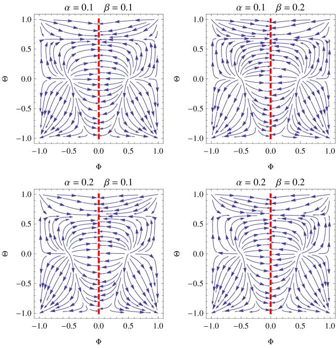
Figure 4: Phase plot of (67), (68) for some $\alpha>0,\beta>0$, $n=2$, and the choice $2C:=\alpha+\sqrt{\alpha^{2}+4\beta}$. The red dashed line is a stable curve of equilibrium points $L:(\phi,\theta)=(0,\theta^{*})$. The physical region is $\Phi\geq 0$.

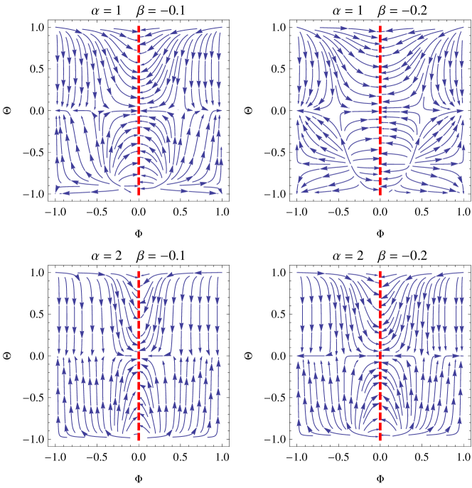
Figure 5: Phase plot of (67), (68) for some $\alpha>0,\beta<0$ and the choice $2C_{-}:=\alpha-\sqrt{\alpha^{2}-4|\beta|}$. The red dashed line is a stable curve of equilibrium points $L:(\phi,\theta)=(0,\theta^{*})$. The physical region is $\Phi\geq 0$.

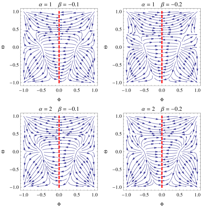
Figure 6: Phase plot of (67), (68) for some $\alpha>0,\beta<0$ and the choice $2C_{+}:=\alpha+\sqrt{\alpha^{2}-4|\beta|}$. The red dashed line is a stable curve of equilibrium points. The physical region is $\Phi\geq 0$.

The asymptotic equations (69), (70) as $\phi\rightarrow 0$ are integrable with solution

$$\left(\begin{array}[c]{c}\phi(\tau)\\ \theta(\tau)\end{array}\right)=\left(\begin{array}[c]{c}e^{-\frac{\tau}{n}}c_{1}\\ \frac{2C-\alpha}{C-\exp\left(\frac{(2C-\alpha)\left(e^{-\tau}c_{1}^{n}+2Cc_{2}\right)}{2C}\right)}\end{array}\right),$$ (71)

converging to $L:(\phi,\theta)=(0,\theta^{*})$ as $\tau\rightarrow\infty$ for bounded $\theta$.

Figure 4 shows the phase plot of system (67), (68) for some $\alpha>0,\beta>0$, $n=2$, and the choice $2C:=\alpha+\sqrt{\alpha^{2}+4\beta}$. The red dashed line is a stable line of equilibrium points $L:(\phi,\theta)=(0,\theta^{*})$.

Figure 5 shows the phase plot of system (67), (68) for some $\alpha>0,\beta>0$, $n=2$, and the choice $2C_{-}:=\alpha-\sqrt{\alpha^{2}-4|\beta|}$. The red dashed line is a stable curve of equilibrium points $L:(\phi,\theta)=(0,\theta^{*})$.

Figure 6 shows the phase plot of system (67), (68) for some $\alpha>0,\beta>0$, $n=2$, $\alpha^{2}+4\beta\geq 0$ and the choice $2C_{+}:=\alpha+\sqrt{\alpha^{2}-4|\beta|}$. The red dashed line is a stable curve of equilibrium points $L:(\phi,\theta)=(0,\theta^{*})$.

All these plots illustrate our analytical findings. These are: (i) The solution of (2) $R=-Ct$ defined for $-\infty<t\leq 0$, where $C>0$ is a fixed constant, is unstable. (ii) The curve of equilibrium points $L:(\phi,\theta)=(0,\theta^{*})$ (i.e., $u\rightarrow\infty$, and $v\rightarrow\infty$, in such a way that $1-u+v\rightarrow\theta^{*}$) is stable as $\tau\rightarrow\infty$ for bounded $\theta$.

Result (ii) means that, as $\tau\rightarrow\infty$, we have

$$1-u(\tau)+u^{\prime}(\tau)=\theta^{*},\quad u(\infty)=\infty.$$ (72)

The solution of (72) is

$$u(\tau)=c_{1}e^{\tau}-\theta^{*}+1,\quad c_{1}\neq 0.$$ (73)

Then,

$$\bar{R}(\tau)=R_{s}(\tau)u(\tau)=Ce^{-\tau}u(\tau)=C\left(c_{1}-(\theta^{*}-1)e^{-\tau}\right).$$ (74)

Hence,

$$R(t)=C\left(c_{1}+(\theta^{*}-1)t\right).$$ (75)

Substituting back in (2), we have that in order of (75) to be an exact solution for (2) we must impose the compatibility condition:

$$C\theta^{*}(\alpha+C(\theta^{*}-2))=0.$$ (76)

We have some specific solutions when $\theta^{*}\in\left\{0,2-\frac{\alpha}{C}\right\}$.

However, recall that $\theta^{*}$ is an arbitrary constant value by definition of line $L$. So, the natural condition is

$$C=\frac{\alpha}{2-\theta^{*}}.$$ (77)

Then, the solution of (2) given by

$$R(t)=\frac{\alpha c_{1}}{2-\theta^{*}}+\frac{\alpha(\theta^{*}-1)t}{2-\theta^{*}},\quad c_{1}\neq 0,$$ (78)

defined in the semi-infinite-interval $-\infty<t\leq 0$, is stable as $t\rightarrow 0^{-}$ ($\tau\rightarrow+\infty$). Finally,

$$\lim_{t\rightarrow 0^{-}}R(t)=\frac{\alpha c_{1}}{2-\theta^{*}}\neq 0$$ (79)

by construction.

3 Lie symmetries and singularity analysis

In the following, we discuss the application of Lie’s theory and the singularity analysis for the derivation of exact and analytic solutions for the master equation (2).

3.1 Lie symmetries

Consider the function $\Phi$ which describes the map of an one-parameter point transformation such as $\Phi\left(R\left(t\right)\right)=R\left(t\right)\$with infinitesimal transformation

$$t^{\prime} =t^{i}+\varepsilon\xi\left(t,R\right),$$ (80)

$$R^{\prime} =R+\varepsilon\eta\left(t,R\right)$$ (81)

and generator $\mathbf{X}=\frac{\partial t^{\prime}}{\partial\varepsilon}\partial_{t}+\frac{\partial x^{\prime}}{\partial\varepsilon}\partial_{R},~{}$where $\varepsilon$ is the parameter of smallness; $t$ is the independent variable and $R\left(t\right)$ the dependent variable.

Assume $R\left(t\right)$ be a solution for the differential equation $\mathcal{H}\left(t,R,\dot{R},\ddot{R}\right)=0.$ Then, under the one-parameter map $\Phi$, function $R^{\prime}\left(t^{\prime}\right)=\Phi\left(R\left(t\right)\right)$ is a solution for the differential equation $\mathcal{H}$, if and only if the differential equation is also invariant under the action of the map, $\Phi$, that is, the following condition holds ²⁷

$$\Phi\left(\mathcal{H}\left(t,R,\dot{R},\ddot{R}\right)\right)=0.$$ (82)

For every map $\Phi$ in which condition (82) holds, means that the generator $X$ is a Lie point symmetry for the differential equation, while the following condition is true

$$\mathbf{X}^{\left[2\right]}\left(\mathcal{H}\left(t,R,\dot{R},\ddot{R}\right)\right)=0.$$ (83)

Vector field $\mathbf{X}^{\left[1\right]}$ describes the first extension of the symmetry vector in the jet-space of variables, $\left\{t,R,\dot{R},\ddot{R}\right\}$ defined as

$$X^{\left[2\right]}=X+\eta^{\left[1\right]}\partial_{\dot{R}}+\eta^{\left[2\right]}\partial_{\ddot{R}},$$ (84)

with $\eta^{\left[1\right]}=\dot{\eta}-\dot{R}\xi$ and $\eta^{\left[2\right]}=\dot{\eta}^{\left[1\right]}-\ddot{R}\dot{\xi}$.

The existence of a Lie symmetry for a given differential equation indicates the associated Lagrange’s system, $\frac{dt}{\xi}=\frac{dR}{\eta},~{}$in which the solution of this system provides the invariant functions which can be used to reduce the order of the ordinary differential equation.

Let us now turn our attention to the boundary condition (2). By applying Lie’s theory, it follows that Equation (2) is invariant under the infinitesimal transformation ²⁷

$$\overline{t} \rightarrow t+\varepsilon\left(\alpha_{1}+\alpha_{2}t\right),$$ (85)

$$\bar{R} \rightarrow R+\varepsilon\left(\alpha_{2}R\right),$$ (86)

where $\varepsilon$ is the infinitesimal parameter, that is, $\varepsilon^{2}\simeq 0.~{}$

Hence, equation (2) admits as Lie point symmetries the vector fields $X_{1}=\partial_{t}$ and $X_{2}=t\partial_{t}+R\partial_{R}$, with commutator $\left[X_{1},X_{2}\right]=X_{1}$. The Lie symmetries $\left\{X_{1},X_{2}\right\}$ form the $A_{2,2}$ Lie algebra in the Morozov-Mubarakzyanov classification scheme ⁴². We continue by applying the corresponding Lie invariants to reduce the order of the master equation (2).

From the Lie point symmetry $X_{1}$ we define the differential invariants$~{}y=\dot{R}~{},~{}x=R$. Thus, by assuming $x$ to be the new independent variable and $y=y\left(x\right)$, equation (2) is written as

$$2xy\frac{dy\left(x\right)}{dx}+y^{2}\left(x\right)+\alpha y\left(x\right)-\beta=0~{}.$$ (87)

Equation (87) admits the Lie symmetry vector $\Gamma^{1}=\left(y\left(x\right)+\alpha y-\frac{\beta}{y\left(x\right)}\right)\partial_{y}$ which provides the Lie’s integration factor $\mu=\left(2x\left(y^{2}\left(x\right)+\alpha y-\beta\right)\right)^{-1}$; hence, by multiply equation (87) with it we end with the equation

$$\int\frac{y}{\left(y^{2}+\alpha y-\beta\right)}dy=-\frac{dx}{2x},$$ (88)

that is,

$$\ln\left(x-x_{0}\right)=-\ln\left(y^{2}+\alpha y-\beta\right)-\frac{2\alpha}{\sqrt{\alpha^{2}+4\beta}}\text{arctanh}\left(\frac{2y+\alpha}{\sqrt{\alpha^{2}+4\beta}}\right).$$ (89)

When $\beta=-\frac{\alpha^{2}}{4}$, solution (89) is written

$$\ln\left(2+y+\alpha\right)+\frac{\alpha}{2y+\alpha}=-\frac{1}{2}\ln\left(x-x_{0}\right).$$ (90)

Moreover, application of the symmetry vector $X_{2}$ in (2) provides the first-order ordinary differential equation

$$2z\left(y\left(z\right)-z\right)\frac{dy\left(z\right)}{dz}+y^{2}\left(z\right)+\alpha y\left(z\right)-\beta=0.$$ (91)

The latter equation belongs to the family of Abel equations of the second kind. Equation (91) can be integrated similarly with equation (87) with the derivation of Lie’s integration factor. For a constant value $y=y_{0}$, with $y_{0}^{2}+\alpha y_{0}-\beta=0$ it is clear that the exact solution of ²³ is recovered.

3.2 Singularity analysis

The ARS algorithm ^{35, 36, 37} has three basic steps which we briefly discuss. The first step is based on the determination of  the leading-order behavior, at least in terms of the dominated exponent. The coefficient of the leading-order term may or may not be explicit. This indicates the existence of a movable singularity for the given differential equation. A second step is the determination of the exponents at which the arbitrary constants of integration enter. This step provides information about the existence of integration constants for the differential equation. Finally, the third step is called the consistency test, where we substitute an expansion up to the maximum resonance into the full equation to check if solves the equation.

For the singularity analysis to work the exponents of the the leading-order term needs to be a negative integer or a nonintegral rational number, while the resonances should be rational numbers, while one of the resonances should be $-1\,\$which warranty the singularity is a movable pole. Excluding the generic resonance $-1$, the analytic solution is expressed by a Right Painlevé Series if the rest of the resonances are nonnegative, for a Left Painlevé Series the resonances must be nonpositive while for a full Laurent expansion the resonances they have to be mixed. Clearly for a second-order ordinary equation  the possible Laurent expansions are Left or Right Painlevé Series.

We apply the ARS algorithm for equation (2), from the fist stem we determine the leading-order term to be $R_{\text{leading}}\left(t\right)=R_{0}\left(t-t_{0}\right)^{\frac{2}{3}}$, where $t_{0}$ indicates the location of the movable singularity and $R_{0}$ is arbitrary. From the second step, the resonances, are derived to be $s_{1}=-1$ and $s_{4}=4$, which means that the analytic solution of (2) can be expressed in terms of the Right Painlevé Series

$$R\left(t\right)=R_{0}\left(t-t_{0}\right)^{\frac{2}{3}}+R_{1}\left(t-t_{0}\right)+R_{2}\left(t-t_{0}\right)^{\frac{4}{3}}+R_{3}\left(t-t_{0}\right)^{\frac{5}{3}}+\ldots~{}.$$ (92)

We replace in (2) from where we find that

$$R_{1}=-\frac{3\alpha}{4},~{}R_{2}=\frac{9}{320R_{0}}\left(3\alpha^{2}+16\beta\right),~{}R_{2}=\frac{3\alpha}{320R_{0}^{2}}\left(3\alpha^{2}+16\beta\right),\ldots.$$ (93)

In the special case in which $\left(3\alpha^{2}+16\beta\right)=0$, that is $\beta=-\frac{3\alpha^{2}}{16}$, we find that $R_{I}=0,~{}I>1$, thus we end with the closed-form solution

$$R_{s}\left(t\right)=R_{0}\left(t-t_{0}\right)^{\frac{2}{3}}-\frac{3\alpha}{4}\left(t-t_{0}\right),\quad\beta=-\frac{3\alpha^{2}}{16},$$ (94)

which can be seen as extension of the exact solution of ²³. Indeed for large values of $t-t_{0}$, $R_{s}\left(t\right)\simeq-\frac{3\alpha}{4}\left(t-t_{0}\right)$, however, for small values of $\left(t-t_{0}\right)$, the term $\left(t-t_{0}\right)^{\frac{2}{3}}$ dominates such that $R_{s}\left(t\right)\simeq R_{0}\left(t-t_{0}\right)^{\frac{2}{3}}$.

It is clear that from the symmetry analysis and the singularity analysis new exact solutions were found for the master equation (2).

4 Conclusions

We performed a detailed study for the master equation of the temporal equation of radiating stars by investigating the global dynamics, the Lie point symmetries and applying the ARS algorithm of singularity analysis. From the analysis of the global dynamics of the master equation we were able to find a new asymptotic behavior which corresponds to a new exact solution for a radiating star spacetime, as also to extract important information to infer about the stability and the physical properties of the asymptotic solutions.

We have new analytical findings. The solution of (2) $R=-Ct$ defined for $-\infty<t\leq 0$, where $c_{1}>0$ is a fixed constant, is unstable. The curve of equilibrium points $L:(\phi,\theta)=(0,\theta^{*})$ has associated a family of solutions of (2) given by (78), defined in the semi-infinite-interval $-\infty<t\leq 0$, which is stable as $t\rightarrow 0^{-}$ ($\tau\rightarrow+\infty$). Furthermore, the Lie symmetry analysis provides that the master equation admits two Lie point symmetries which form the $A_{2,2}$ Lie algebra. Each Lie symmetry was applied to reduce the order for the ordinary differential equation into a first-order differential equation, while new exact similarity solutions were found.

Finally, from the application of the ARS algorithm, we found that the master equation possesses the Painlevé property and we were able to write the analytic solution for the radiating stars in order of Painlevé Series (92), where $R_{0}$ is arbitrary, $R_{1}$ is function of $\alpha$, and the $R_{j},j\geq 2$ are functions of parameters $\alpha$ and $\beta$. Additionally, we have obtained the closed-form solution (94) for $\beta=-\frac{3\alpha^{2}}{16}$. To summarise, we have investigated the global dynamics for the given master ordinary differential equation to understand the evolution of solutions for various initial conditions as also to investigate the existence of asymptotic solutions. Moreover, with the application of Lie’s theory, we have reduced the order of the master differential equation, while an exact similarity solution was determined. Finally, the master equation possesses the Painlevé property. Therefore, the analytic solution can be expressed in terms of a Laurent expansion. Such analyses are essential for understanding the physical properties of spacetimes which describe radiating stars.

CONFLICT OF INTEREST

The authors declare to have no conflict of interest.

ORCID

Genly Leon https://orcid.org/0000-0002-1152-6548

Megandhren Govender https://orcid.org/0000-0001-6110-9526

Andronikos Paliathanasis https://orcid.org/0000-0002-9966-5517

References

- 1 J. R. Oppenheimer and H. Snyder, On Continued gravitational contraction, Phys. Rev. 56 (1939), 455-459 doi:10.1103/PhysRev.56.455
- 2 J. Q. Guo, L. Zhang, Y. Chen, P. S. Joshi and H. Zhang, Strength of the naked singularity in critical collapse, Eur. Phys. J. C 80 (2020) no.10, 924 doi:10.1140/epjc/s10052-020-08486-7
- 3 Y. C. Ong, Space–time singularities and cosmic censorship conjecture: A Review with some thoughts, Int. J. Mod. Phys. A 35 (2020) no.14, 14 doi:10.1142/S0217751X20300070
- 4 R. Shaikh and P. S. Joshi, Can we distinguish black holes from naked singularities by the images of their accretion disks?, JCAP 10 (2019), 064 doi:10.1088/1475-7516/2019/10/064
- 5 S. M. Wagh and S. D. Maharaj, Naked singularity of the Vaidya-de Sitter space-time and cosmic censorship conjecture, Gen. Rel. Grav. 31 (1999), 975-982 doi:10.1023/A:1026675313562
- 6 K. Akiyama et al. [Event Horizon Telescope], First M87 Event Horizon Telescope Results. I. The Shadow of the Supermassive Black Hole, Astrophys. J. Lett. 875 (2019), L1 doi:10.3847/2041-8213/ab0ec7
- 7 P. C. Vaidya, The gravitational field of a radiating star, Proc. Indian Acad. Sci. (Math. Sci.) 33, 264 (1951) doi:10.1007/BF03173260
- 8 W. B. Bonnor, A. K. G. de Oliveira and N. O. Santos, Radiating spherical collapse, Phys. Rep. 181, 269 (1989) doi: 10.1016/0370-1573(89)90069-0
- 9 L. Herrera and N. O. Santos, Local anisotropy in self-gravitating systems, Phys. Rept. 286 (1997), 53-130 doi:10.1016/S0370-1573(96)00042-7
- 10 N. O. Santos, Non-adiabatic radiating collapse, M.N.R.A.S. 216 (1985), 403-410 doi: 10.1093/mnras/216.2.403
- 11 S. D. Maharaj and B. Brassels, Radiating stars with composite matter distributions, Eur. Phys. J. C 81 (2021), 366 doi: 10.1140/epjc/s10052-021-09163-z
- 12 N. F. Naidu, R. S. Bogadi, A. Kaisavelu and M. Govender, Stability and horizon formation during dissipative collapse, Gen. Relativ. Grav. 52, 79 (2020) doi: 10.1007/s10714-020-02728-5
- 13 L. Herrera, A. di Prisco, E. Fuenmayor and O. Troconis, Dynamics of Viscous Dissipative Gravitational Collapse:. a Full Causal Approach, IJMP-D 18, 129 (2009) doi: 10.1142/S0218271809014285
- 14 R. Chan, L. Herrera and N. O. Santos, Dynamical instability for shearing viscous collapse, M.N.R.A.S 267 (1994), 637-646 doi: 10.1093/mnras/267.3.637
- 15 L. Herrera, A. Di Prisco, J. Ospino, On the stability of the shear–free condition, Gen. Relativ. Gravit. 42 (2010), 1585–1599 doi:10.1007/s10714-010-0931-6
- 16 M. Govender, Nonadiabatic spherical collapse with a two-fluid atmosphere, Int. J. Mod. Phys. D. 22 (2013), 1350049 doi.org/10.1142/S0218271813500491
- 17 B. V. Ivanov, A different approach to anisotropic spherical collapse with shear and heat radiation, Int. J. Mod. Phys. D. 25 (2015), 1650049 doi: 10.1142/S0218271816500498
- 18 B. V. Ivanov, Generating solutions for charged geodesic anisotropic spherical collapse with shear and heat radiation, Eur. Phys. J. C, 79 (2019), 255 doi.org/10.1140/epjc/s10052-019-6772-x
- 19 A. Banerjee, S. Chatterjee and N. Dadhich, Spherical collapse with heat flow and without horizon, Mod. Phys. Lett. A 17 (2002), 2335-2340 doi:10.1142/S0217732302008320
- 20 K. S. Govinder and M. Govender, A General Class of Euclidean Stars, Gen. Relativ. Gravit. 44 (2012), 147-156 doi: 10.1007/s10714-011-1268-5
- 21 R. Chan, Radiating gravitational collapse with shear viscosity, M.N.R.A.S 316 (2000), 588 doi.org/10.1046/j.1365-8711.2000.03547.x
- 22 G. Pinheiro and R. Chan, Radiating gravitational collapse with shearing motion and bulk viscosity revisted, Int. J. Mod. Phys. D. 19 (2012), 11 doi: 10.1142/S0218271810018050
- 23 A. Banerjee, S.B. Duttachoudhury and B.K. Bhui, Conformally flat solution with heat flux, Phys. Rev D 40, 670 (1989) doi: 10.1103/PhysRevD.40.670
- 24 A. Paliathanasis, M. Govender and G. Leon, Temporal evolution of a radiating star via Lie symmetries, Eur. Phys. J. C 81 (2021) no.8, 718 doi:10.1140/epjc/s10052-021-09521-x
- 25 S. D. Maharaj, A. K. Tiwari, R. Mohanlal and R. Narain, J. Math Phys., 57 (2016), 092501https://doi.org/10.1063/1.4961929
- 26 G. Z. Abebe, S. D. Maharaj, K. S. Govinder Gen Relativ Gravit, 46 (2014), 1733 doi: 10.1007/s10714-013-1650-6
- 27 G.W. Bluman and S. Kumei, Symmetries and Differential Equations, Springer-Verlag, New York, (1989)
- 28 L. Kaur and A. M. Wazwaz, Einstein’s vacuum field equation: Painlevé analysis and Lie symmetries, Waves in Random and Complex Media, 31:2, 199-206 (2021), doi: 10.1080/17455030.2019.1574410
- 29 T. Christodoulakis, N. Dimakis and P. A. Terzis, Lie point and variational symmetries in minisuperspace Einstein gravity, J. Phys. A 47 (2014), 095202 doi:10.1088/1751-8113/47/9/095202
- 30 S. Cotsakis, P.G.L. Leach and H. Pantazi, Symmetries of homogeneous cosmologies, Grav. Cosmol. 4 (1998), 314-325 https://ui.adsabs.harvard.edu/abs/1998GrCo....4..314C
- 31 R. Mohanlal, S. D. Maharaj, A. K. Tiwari and R. Narain, Radiating stars with exponential Lie symmetries, Gen. Rel. Grav. 48 (2016), 87 doi:10.1007/s10714-016-2081-y
- 32 G. Z. Abebe and S. D. Maharaj, Charged radiating stars with Lie symmetries, Eur. Phys. J. C 79 (2019) no.10, 849 doi:10.1140/epjc/s10052-019-7383-2
- 33 M. Tsamparlis and A. Paliathanasis, Symmetries of Differential Equations in Cosmology, Symmetry 10 (2018) no.7, 233 doi:10.3390/sym10070233
- 34 R. Conte and M. Musette, The Painlevé Handbook, Springer Netherlands, Amsterdam, Springer Science (2008)
- 35 M.J. Ablowitz, A. Ramani and H. Segur, Nonlinear evolution equations and ordinary differential equations of painlevè type. Lett. Nuovo Cimento 23, 333–338 (1978) doi: 10.1007/BF02824479
- 36 M.J. Ablowitz, A. Ramani and H. Segur, A connection between nonlinear evolution equations and ordinary differential equations of P-type. I, J. Math. Phys. 21, (1980), 715-721 doi: 10.1063/1.524491
- 37 M.J. Ablowitz, A. Ramani and H. Segur, A connection between nonlinear evolution equations and ordinary differential equations of P-type. II, J. Math. Phys. 21 (1980), 1006-1015 doi:10.1063/1.524548
- 38 S. Kowalevski, Sur la problème de la rotation d’un corps solide autour d’un point fixe, Acta Math. 12, 177-232 (1889)
- 39 A. R. Liddle and R. J. Scherrer, A Classification of scalar field potentials with cosmological scaling solutions, Phys. Rev. D 59 (1999), 023509 doi:10.1103/PhysRevD.59.023509
- 40 J. P. Uzan, Cosmological scaling solutions of nonminimally coupled scalar fields, Phys. Rev. D 59 (1999), 123510 doi:10.1103/PhysRevD.59.123510
- 41 B. Aulbach, Continuous and Discrete Dynamics near Manifolds of Equilibria (Lecture Notes in Mathematics No. 1058, Springer, 1984)
- 42 V.V. Morozov, Classification of six-dimensional nilpotent Lie algebras, Izvestia Vysshikh Uchebn Zavendeniĭ Matematika, 5, 161 (1958)