Strange stars in $f(\mathcal{R})$ gravity Palatini formalism and gravitational wave echoes from them

Abstract

The compact stars are promising candidates associated with the generation of gravitational waves (GWs). In this work, we study a special type of compact stars known as strange stars in the $f(\mathcal{R})$ gravity Palatini formalism. Here we consider three promising $f(\mathcal{R})$ gravity models viz., Starobinsky, Hu-Sawicki and Gogoi-Goswami models in the domain of MIT Bag model and linear equations of state (EoSs). We compute the stellar structures numerically and constrained the $f(\mathcal{R})$ model parameters with a set of probable strange star candidates. The study shows that the consideration of stiffer MIT Bag model and linear EoSs within a favourable set of $f(\mathcal{R})$ gravity model parameters may result in strange stars with sufficient compactness to produce echoes of GWs. Thus, we have computed the GWs echo frequencies and characteristic echo times for such stars. It is found that in compliance with the experimentally obtained possible strange star candidates, the obtained GW echo frequencies for all the models are in the range of $65-85$ kHz.

I Introduction

From the current astrophysical and cosmological points of view, we are living in the era of accelerated expansion of the universe Spergel_2007 ; Astier_2006 as well as in the mystery of missing mass in the universe nashelski . There are two general hypotheses to explain this present accelerated expansion of the universe. According to one hypothesis, Einstein’s theory of general relativity (GR) requires the existence of some exotic energy, called the dark energy to explain this current state of the universe Riess_1998 ; perl . In contrast, as per the second hypothesis the need for such an exotic energy can be avoided by extending the geometric part of the GR, usually referred to as the modified theories of gravity (MTGs), for the reason that it is feasible to obtain the present accelerated universe without the necessity of such an illusive exotic energy (detailed review can be found in cappo ). Similarly, the enigma of the missing mass of the universe has been explained by introducing a non-luminous and non-baryonic unknown form of matter, dubbed as the dark matter berton . However, from the perspective of the MTGs this missing mass can be explained without the need of the idea of dark matter Bohmer ; Parbin . Besides these, there are well-known observational and theoretical facts that compel us to study MTGs harko ; nojiri . In fact, currently MTGs are viewed hopefully as a good approach to go beyond GR clifton ; nojiri2 .

To point out new physics from MTGs under the extreme relativistic effects, which are harder to achieve from the earth-based experiments, the compact stars give an excellent platform to do so. It is because of their unique high matter densities than the other nuclear matters. The family of compact objects mainly includes neutron stars and white dwarfs glendeinng ; shapiro . Such objects are the remnant of luminous stars, i.e. the endpoint of their stellar evolution. The family of such stars is now extended to include some more hypothetical stars, such as the strange stars aclock , hybrid stars alford , gravastars visser , boson stars jetzer , axion stars braaten , and other compact exotic stars [e.g. see dejan ]. Compared to other compact stars, by assumption, strange stars have a stable configuration and as such, perhaps they are composed of a matter that may be the true ground state of the hadronic matter witten ; farhi . Due to their unique mass-radius (M-R) relations, they are gaining the utmost interest in recent days. In white dwarfs and neutron stars, the degeneracy pressures are due to electrons and neutrons respectively. This degeneracy pressure is balanced by gravitational force to give a stable configuration to the star. If neutron stars get squeezed at a high temperature, decomposition of neutrons into component quarks occurs baym . Such stars made of quark matter or de-confined quarks are known as the strange stars alcock ; haensel . Since they are in a much more stable configuration in comparison with neutron stars, so the proper understanding of these stars may lead to explain the origin of the huge amount of the energy released in super-luminous supernovae, which occur in about one out of every 1000 supernovae explosions, and they are 100 times more luminous than regular supernovae ofek ; ouyed .

Literature surveys show that various authors have been studying the strange stars and their stellar structures in the realm of GR overgard ; lopeZ ; Maurya ; jb2 . The properties of such compact stars have also been studied in the framework of MTGs by a number of authors maurya ; pano ; stay ; deb ; pretel ; bhar ; biswas ; rej ; hendi ; panah ; asta . Such studies of compact stars in MTGs might allow one to impose constraints on the parameters responsible for the strong field regime, which are expected to break down in GR consideration. It needs to mention that the $f(\mathcal{R})$ gravity models in Palatini formalism are found to pass the astrophysical tests like post-Newtonian (solar system), parametrized post-Newtonian tests, etc. olmo05 ; Olmo . These theories are compatible with the current gravitational wave (GW) observations having good phenomenology in black holes 11olmo ; 12olmo ; bejarano , wormholes bambi ; 16olmo , and stellar structures olmo19 ; kainu ; panotopoulos . An important aspect of application of $f(\mathcal{R})$ gravity models that are designed to describe a low curvature phenomenon to the field of compact stellar study is that such models permit the presence of more massive compact stellar objects as compared to standard GR harko ; goswami . GR gives the maximal mass limit of compact star as $2\,M_{\odot}$ berti ; bhatti ; 20olmo , while there are some more massive stellar structures exceeding the GR limit nice ; van ; rhoa ; kalo ; alsi . Another motivation behind choosing $f(\mathcal{R})$ gravity models in high curvature regimes is that although the data available from the strong curvature regime phenomena are compatible with the GR, there are some issues related to such data which seem to complying with the $f(\mathcal{R})$ and other MTGs kono ; vainio . Moreover, at the astrophysical scales there are some persistent issues of observed massive pulsars which can hardly be explained within the GR limit grigorian ; lenzi ; lihu . So a possible way for getting over these observational issues are MTGs. Interestingly compact objects like neutron stars and strange stars are indeed good tools to test and/or constrain MTGs. Thus it can be conjectured that the strong gravity regimes are some important tools to check the viability of different MTG models psaltis . Previously, compact stars in $f(\mathcal{R})$ theories of gravity in the Palatini formalism have been investigated in Refs. kainu ; olmo ; pannia ; panotopoulos ; Silveira . In Ref. panotopoulos , G. Panotopoulos studied the structure of strange stars by considering two models of $f(\mathcal{R})$ theories viz., the Starobinsky model: $f(\mathcal{R})=\mathcal{R}+\mathcal{R}^{2}/(6\mathcal{M}^{2})$ and the $1/\mathcal{R}$ model with a constant trace $T$ of the energy-momentum tensor $T_{\mu\nu}$. He showed that the behaviour of strange stars varies depending on the model type panotopoulos . Recently, Silveira et. al. studied Silveira the compact and ultra-compact objects considering a Schwarzschild type homogeneous star and by adding a transition zone for the density near the surface of star in the $f(\mathcal{R})$-Palatini theory. In GR the asteroseismological behaviours of strange stars are studied in jb and also the GW echo frequencies emitted by such stars are reported earlier in pani ; manarelli ; urbano ; jb ; zhang . Motivated by these works, in this present work we have used constant as well as variable trace $T$ of the energy-momentum tensor $T_{\mu\nu}$ to see how the structure of such stars depends on models of the $f(\mathcal{R})$ gravity in Palatini formalism. We have considered three concrete and viable $f(\mathcal{R})$ gravity models i.e., the Starobinsky model staro , the Hu-Sawicki model hu , and the newly introduced model in gg . It needs to be mentioned that we consider this new model with the other two well-known models in the field of MTGs to validate the new model in the astrophysical context. Hereafter, for the convenient representation we will call this model as the Gogoi-Goswami model. Using the modified Tolman-Oppenheimer-Volkoff (TOV) equations for the $f(\mathcal{R})$ gravity along with three equations of state (EoSs) viz., the MIT Bag model EoS, the stiffer MIT Bag model EoS and the linear EoS, we found the stellar structure solutions. We have constrained these models using a set of possible strange stars candidates. Also, for the first time in this work we have determined the GW echo frequencies emitted by these ultra-compact objects in the $f(\mathcal{R})$ gravity Palatini formalism.

After this brief introduction, we have organized our article as follows. In section II, the $f(\mathcal{R})$ gravity theory in Palatini formalism and the concerned models of this gravity are discussed very shortly. The modified TOV equations are derived and the method of their corresponding solutions for the considered models are also discussed in this section. A workable introduction of GW echoes is given in the section III. In section IV, the numerical results of our work are presented. Finally, we conclude our article in the section V. In this article, we adopt the unit of $c=G=1$, where $c$ and $G$ denote the speed of light and the gravitational constant respectively, and also we used the metric signature $(-,+,+,+)$.

II Ultracompact stars in modified theories of gravity

In this section, first we shall briefly summarize the $f(\mathcal{R})$ theories of gravity in the Palatini formalism and then shall derive the modified TOV equations in this theory. These TOV equations are then numerically solved for the three viable $f(\mathcal{R})$ gravity models using the three EoSs as mentioned in the previous section to study the properties of strange stars.

In Palatini $f(\mathcal{R})$ theories the action is given by

$$S=\dfrac{1}{16\pi}\int d^{4}x\,\sqrt{-g}f(\mathcal{R})+\int d^{4}x\sqrt{-g}\,\mathcal{L}_{m}(g_{\mu\nu}),$$ (1)

where $\mathcal{L}_{m}$ is the matter Lagrangian density and $f(\mathcal{R})$ is the generic function of the Ricci scalar. Varying this action with respect to both the metric $g_{\mu\nu}$ and the affine connection $\Gamma^{\rho}_{\mu\nu}$, the field equations can be obtained in the form kainu :

$$F(\mathcal{R})\mathcal{R}_{\mu\nu}-\dfrac{1}{2}f(\mathcal{R})g_{\mu\nu}=8\pi T_{\mu\nu},$$ (2)

$$\nabla_{\rho}\!\left(\sqrt{-g}F(\mathcal{R})g^{\mu\nu}\right)=0.$$ (3)

Here $F\equiv\partial f/\partial\mathcal{R}$, $\mathcal{R}\equiv g^{\mu\nu}\mathcal{R}_{\mu\nu}(\Gamma)$ and $T_{\mu\nu}$ is the energy-momentum tensor of $\mathcal{L}_{m}$. Taking the trace of equation (2), a purely algebraic equation relating $\mathcal{R}$ and $T$ can be obtained as

$$F(\mathcal{R})\mathcal{R}-2f(\mathcal{R})=8\pi T.$$ (4)

If we consider the perfect fluid model for the materials of stars, the trace of $T_{\mu\nu}$ can be obtained as $T=-\,\rho+3p$ with the pressure $p$ and the energy density $\rho$. Again, in order to describe a spherically symmetric spacetime, we use the metric represented by the line element:

$$ds^{2}=-f(r)\,dt^{2}+g(r)\,dr^{2}+r^{2}d\Omega^{2},$$ (5)

where the unknown metric functions $f(r)$ and $g(r)$ are dependent on the radial coordinate $r$ only. $d\Omega^{2}=d\theta^{2}+\sin^{2}\theta\,d\phi^{2}$ with $\theta$ and $\phi$ are the polar angle and the azimuth angle respectively. Considering the exterior to the stars be the vacuum with $T_{\mu\nu}=0$, the exterior solutions for our considered models are found to be the Schwarzchild (de-Sitter if $\Lambda_{0}>0$ or anti-de-Sitter if $\Lambda_{0}<0$) solutions as given by

$$f(r)=g(r)^{-1}=1-\dfrac{2M}{r}{-\dfrac{\Lambda_{0}}{3}r^{2}}.$$ (6)

Whereas the interior solutions in this theory give,

$$f(r)=g(r)^{-1}=1-\dfrac{2m(r)}{r}-\dfrac{\Lambda_{\rho}}{3}r^{2}.$$ (7)

Here $M$ is the total mass of stars with the radius $R$ and $m(r)$ is their mass at the radial distance $r<R$. $\Lambda_{\rho}$ is the effective cosmological constant inside the stars, which arises due to the curvature function $f(\mathcal{R})$ of the theory and is given by

$$\Lambda_{\rho}=\dfrac{1}{2}\left(\mathcal{R}-\dfrac{f(\mathcal{R})}{F(\mathcal{R})}\right).$$ (8)

Upon matching the exterior and interior solutions at $r=R$, we can obtain the total mass of stars as kainu ; panotopoulos

$$M=m(R)+\dfrac{(\Lambda_{\rho}{-\Lambda_{0}})R^{3}}{6}.$$ (9)

It is to be noted that the vacuum value of the effective cosmological constant $\Lambda_{0}$ outside the star vanishes for our considered models. Thus, for our models equation (9) will take the form:

$$M=m(R)+\dfrac{\Lambda_{\rho}R^{3}}{6}.$$ (10)

One can see that the curvature modification has a contribution to the total mass of stars in the theory depending on the type of a model. The bare mass $m(R)$ in this mass equation can be calculated from the modified TOV equations given below. Now, to be more specific we consider $g(r)=e^{\lambda(r)}$ and $f(r)=e^{\chi(r)}$, where $\lambda(r)$ and $\chi(r)$ are two source functions of $r$. For the line element (5) with these specific forms of $f(r)$ and $g(r)$, the tt- and rr-components of field equations (2) and (3) give the equations for functions $\lambda(r)$ and $\chi(r)$ as

$$\lambda^{\prime}(r) =\dfrac{1}{1+\gamma}\left(\dfrac{1-e^{\lambda}}{r}+\dfrac{\alpha+\beta}{r}+8\pi r\rho\,\dfrac{e^{\lambda}}{F}\right),$$ (11)

$$\chi^{\prime}(r) =-\dfrac{1}{1+\gamma}\left(\dfrac{1-e^{\lambda}}{r}+\dfrac{\alpha}{r}-8\pi rp\,\dfrac{e^{\lambda}}{F}\right),$$ (12)

where the prime denotes the derivative with respect to $r$ and

$$\alpha=r^{2}\left[\dfrac{4}{3}\left(\dfrac{F^{\prime}}{F}\right)^{2}+\dfrac{2}{r}\dfrac{F^{\prime}}{F}+\dfrac{e^{\lambda}}{2}\left(\mathcal{R}-\dfrac{f}{F}\right)\right],\;\;\beta=r^{2}\left[\dfrac{F^{\prime\prime}}{F}-\dfrac{3}{2}\left(\dfrac{F^{\prime}}{F}\right)^{2}\right],\;\;\mbox{and}\;\;\gamma=\dfrac{rF^{\prime}}{2F}.$$ (13)

For a star in hydrostatic equilibrium the interior solution is described by the famous TOV equations tolman ; tov . The solutions of these equations can lead one to know the physical properties like mass, pressure and radius of the star. These TOV equations will take the modified form in MTGs in comparison to their form in GR. The modified TOV equations for the $f(\mathcal{R})$ gravity in the Palatini formalism are found as kainu

$$\dfrac{dp}{dr} =-\dfrac{1}{1+\gamma}\dfrac{p+\rho}{r(r-2m)}\left[m+\dfrac{4\pi r^{3}p}{F}-\dfrac{\alpha}{2}(r-2m)\right],$$ (14)

$$\dfrac{dm}{dr} =\dfrac{1}{1+\gamma}\left[\dfrac{4\pi r^{2}\rho}{F}+\dfrac{\alpha+\beta}{2}\dfrac{m}{r}(\alpha+\beta-\gamma)\right].$$ (15)

It is to be noted that when $F=1$, then these equations will take their original form in GR. Moreover, when the trace of the energy-momentum tensor $T(\rho)$ is a constant independent of $r$, then the Ricci scalar $\mathcal{R}$ is also a constant. One should note that the complete field equations equations (2) and (3) take the familiar form of Einstein’s equations with a non-vanishing cosmological constant and with the right side scaled by a $\rho$ dependent constant parameter $F_{\rho}$ kainu as

$$G_{\mu\nu}+\Lambda_{\rho}g_{\mu\nu}=\dfrac{8\pi}{F_{\rho}}\,T_{\mu\nu}.$$ (16)

Here $F_{\rho}$ is the derivative of $f(\mathcal{R})$ with respect to $\mathcal{R}$ evaluated at the constant value $\mathcal{R}_{0}$ that solves the trace equation (equation 4). $\Lambda_{\rho}$ is the effective cosmological constant as given in equation (8) and for a constant trace $T$ it is independent of $r$.

At this moment we are in a position to use the $f(\mathcal{R})$ gravity models of our interest as mentioned earlier. The Starobinsky model with its extended form can be written as staro

$$f_{s}(\mathcal{R})=\mathcal{R}-s\mathcal{M}_{s}^{2}\left[1-{\left(\dfrac{\mathcal{R}^{2}}{\mathcal{M}_{s}^{4}}+1\right)}^{-n}\right],$$ (17)

where $s$, $\mathcal{M}_{s}$ and $n$ are the Starobinsky model parameters. In fact, the parameter $\mathcal{M}_{s}$ is the mass scale and here we consider it as a free parameter. In our work we will use $n=1$, for which the model reduces to the form:

$$f_{s}(\mathcal{R})=\mathcal{R}-s\,\dfrac{\mathcal{R}^{2}}{\mathcal{M}_{s}^{2}}.$$ (18)

The first derivative of the above equation with respect to $\mathcal{R}$ gives,

$$F_{s}(\mathcal{R})=1-2s\dfrac{\mathcal{R}}{\mathcal{M}_{s}^{2}}.$$ (19)

Using this result with the model (18) in the trace equation (4), we can obtain the background curvature

$$\mathcal{R}_{0}=-\,8\pi T.$$ (20)

The second $f(\mathcal{R})$ gravity model considered in this work is the Hu-Sawicki model, which is defined as hu

$$f_{h}(\mathcal{R})=\mathcal{R}-\dfrac{c_{1}\mathcal{M}^{2}_{h}\left(\dfrac{\mathcal{R}}{\mathcal{M}^{2}_{h}}\right)^{\mu}}{c_{2}\left(\dfrac{\mathcal{R}}{\mathcal{M}^{2}_{h}}\right)^{\mu}+1},$$ (21)

where $c_{1}$, $c_{2}$ and $\mathcal{M}_{h}$ are model parameters. The parameters $c_{1}$ and $c_{2}$ are dimensionless in nature, while the third parameter $\mathcal{M}_{h}$ has the dimension of length^-1, which is considered to be a free parameter here. For this model we have,

$$F_{h}(\mathcal{R})=1+\dfrac{c_{1}c_{2}\mu\left(\dfrac{\mathcal{R}}{\mathcal{M}^{2}_{h}}\right)^{2\mu-1}}{\left[1+c_{2}\left(\dfrac{\mathcal{R}}{\mathcal{M}^{2}_{h}}\right)^{\mu}\right]^{2}}.$$ (22)

From the trace equation (4), we can find out the background curvature for this model as given by

$$\mathcal{R}_{0}=\frac{A^{2/3}+B}{3\,c_{2}\,C^{1/3}},$$ (23)

where

$$A =D+192\pi^{2}(2c_{1}+1)c_{2}^{2}\mathcal{M}_{h}^{2}T^{2}-12\pi(c_{1}(8c_{1}-1)+2)c_{2}\mathcal{M}_{h}^{4}T+(c_{1}-1)^{2}(8c_{1}+1)\mathcal{M}_{h}^{6}-512\pi^{3}c_{2}^{3},$$ (24)

$$B =2\,C^{1/3}\left[(c_{1}-1)\mathcal{M}_{h}^{2}-4\pi c_{2}T\right]-16\pi(2c_{1}+1)c_{2}\mathcal{M}_{h}^{2}T+(c_{1}-1)(4c_{1}-1)\mathcal{M}_{h}^{4}+64\pi^{2}c_{1}^{2}T^{2},$$ (25)

$$C =D+12\pi\left(-8c_{1}^{2}+c_{1}-2\right)c_{2}\mathcal{M}_{h}^{4}T+192\pi^{2}(2c_{1}+1)c_{2}^{2}\mathcal{M}_{h}^{2}T^{2}+(c_{1}-1)^{2}(8c_{1}+1)\mathcal{M}_{h}^{6}-512\pi^{3}c_{2}^{3}T^{3}.$$ (26)

$$D =3\mathcal{M}_{h}^{3}\sqrt{-\,3\,c_{1}\big{[}-48\pi^{2}(5c_{1}+4)c_{2}^{2}\mathcal{M}_{h}^{2}T^{2}+24\pi(c_{1}-1)^{2}c_{2}\mathcal{M}_{h}^{4}T+(c_{1}-1)^{3}\mathcal{M}_{h}^{6}+512\pi^{3}c_{2}^{3}T^{3}\big{]}}.$$ (27)

The third viable $f(\mathcal{R})$ gravity model considered in this work is the Gogoi-Goswami model having the form gg :

$$f_{g}(\mathcal{R})=\mathcal{R}-\dfrac{\alpha}{\pi}\,\mathcal{R}_{c}\cot^{-1}\left(\dfrac{\mathcal{R}^{2}_{c}}{\mathcal{R}^{2}}\right)-\beta\,\mathcal{R}_{c}\left[1-\exp\left(-\frac{\mathcal{R}}{\mathcal{R}_{c}}\right)\right],$$ (28)

where $\alpha$ and $\beta$ are two free parameters of the model, and $\mathcal{R}_{c}$ is the characteristic curvature constant with the dimension same as the curvature scalar $\mathcal{R}$. The first derivative of the model with respect to $\mathcal{R}$ is given by

$$F_{g}(\mathcal{R})=1-\frac{2\alpha\mathcal{R}\mathcal{R}_{c}^{3}}{\pi\mathcal{R}^{4}+\pi\mathcal{R}_{c}^{4}}-\beta e^{-\frac{\mathcal{R}}{\mathcal{R}_{c}}}.$$ (29)

In case of this model, the trace equation (4) takes the following form:

$$\mathcal{R}_{c}\left[x\left(-\frac{2\,\alpha\,x}{\pi x^{4}+\pi}-\beta e^{-x}-1\right)+\frac{2\alpha\tan^{-1}(x^{2})}{\pi}+2\beta\left(\sinh(x)-\cosh(x)+1\right)\right]=8\pi T,$$ (30)

where $x=\mathcal{R}/\mathcal{R}_{c}$ is a dimensionless variable. This equation can’t be solved analytically and hence we have to implement a numerical method to solve the same. For this purpose, we define two functions as

$$f_{g}(x) =x\left(-\frac{2\alpha x}{\pi x^{4}+\pi}-\beta e^{-x}-1\right)+\frac{2\alpha\tan^{-1}(x^{2})}{\pi},$$ (31)

$$g_{g}(x) =\frac{8\pi T}{\mathcal{R}_{c}}-2\beta\,\left[\sinh(x)-\cosh(x)+1\right],$$ (32)

where $x$ can be a solution of equation (30) provided

$$\big{|}f_{g}(x)-g_{g}(x)\big{|}\approx 0.$$

Further, to describe the ultra compact stars, in particular strange stars we shall consider three EoSs. The first one is the MIT Bag model EoS, which was proposed to explain a relativistic gas of massless de-confined quarks witten ; chodosa ; chodosb ; jb and is given by

$$p=\dfrac{1}{3}(\rho-4B).$$ (33)

Here $p$ is the perfect fluid pressure, $\rho$ is the fluid density and $B$ is the Bag constant. The constant $B$ may have different possible values, which have been discussed in detail in Ref. jb . In this work we shall use a suitable value of $B=(168MeV)^{4}$. This value is chosen in such a way that it lies in the acceptable range aziz and the solutions obtained with this value are such that they do not exceed the mass and radius of $\approx 3\,\mbox{M}_{\odot}$ and $\approx 13\,\mbox{km}$ respectively for all the considered cases in the present study. This mass and radius bound is taken in such a way that we will get physically stable strange star configurations in our study. However, to obtain the stellar properties, especially the property that is suitable to get GW echoes from the stars, we have also chosen the stiffer form of this EoS manarelli ; jb as given by

$$p=(\rho-4B).$$ (34)

The third EoS considered in this work is the linear EoS dey having the form:

$$p=b(\rho-\rho_{s}),$$ (35)

where $b$ is the linear constant and $\rho_{s}$ is the surface energy density of the star. As in the case of the MIT Bag model EoS, for this EoS also we have taken a suitable value of $b=0.910$ jb in this work. By fixing some EoSs the TOV equations (in GR or in MTGs) can be solved numerically, which will lead to know the structure of the compact object under consideration. Thus with these three EoSs we have solved numerically the TOV equations in the $f(\mathcal{R)}$ gravity models of Starobinsky, Hu-Sawicki and Gogoi-Goswami in the Palatini formalism. Using the solutions of these stellar structure equations, finally we have calculated the GW echo frequencies emitted by such stars.

From an EoS we can have a specific form of the energy-momentum trace, which can be used in the expression of the background curvature for each $f(\mathcal{R})$ gravity model to obtain a specific form for its background curvature. In the case of the MIT Bag model (equation (33)), the trace of the energy-momentum $T$ is a constant quantity leading to a simple situation. While for the stiffer form of the MIT Bag model EoS (equation (34)) the energy-momentum trace $T=2\,\rho-12B$ and for the linear EoS (equation (35)) it is $T=(3\,b-1)\rho-3\rho_{s}$. Thus, using these EoSs in the modified TOV equations (14) and (15), and also using the considered $f(\mathcal{R)}$ gravity models with the initial conditions: $m(r=0)=0$ and $p(r=0)=p_{c}$, we can solve them numerically. In addition the bare mass $m(R)$ and the radius $R$ of a star can be determined by the boundary conditions: $m(r=R)=m(R)$ and $p(r=R)=0$.

One should note that the gravitational field for strange stars is sourced by the trace of the energy-momentum tensor as given by equation (4). In the usual case, for the Sun like stars the pressure to density ratio is very small ($\approx 10^{-9}$) and so it is possible to neglect the pressure for non-relativistic stars while calculating the metric. But in the case of stars with high compactness such as strange stars, we can not neglect the pressure term, which increases the complexity of the problem. However, in the case of the standard MIT Bag model, we have $T=constant$, which makes the situation less complex. One may note here that $T=constant$ does not imply that the density of a star is constant throughout the whole region, but instead it indicates that any variation in the pressure and density of the star does not influence the trace of the energy-momentum tensor. So, undoubtedly this is an ideal standard case in the $f(\mathcal{R})$ gravity, which makes the situation comparatively simple enough to handle. The complexity increases when we move to the other EoSs, where the trace of the energy-momentum tensor is not constant, i.e. any variation in the pressure and density of a star can impact the trace of the energy-momentum tensor significantly. We have seen that a viability condition $\big{|}F(\mathcal{R})-1\big{|}\ll 1$ makes the system solvable under suitable approximations. Another thing to consider is the matching of exterior and interior solutions i.e., while solving field equations of $f(\mathcal{R})$ gravity, junction conditions must be considered for the smooth matching of interior and exterior spacetimes Olmo . In GR, these boundary conditions are known as the Darmois-Israel matching or junction conditions israel ; darmois . In the Ref. Olmo the authors utilized the tensor distributional technique to find the junction conditions for Palatini $f(\mathcal{R})$ gravity. It is shown that these junction conditions are required to build the stellar models of gravitational bodies with the matching of interior and exterior regions at some hypersurfaces. They have considered the stellar surfaces in the polytropic models in the Palatini framework as an example and their results showed that the white dwarfs and neutron stars can be modelled safely within this framework. For the smooth matching of our exterior and interior solutions on the stellar surface, we consider a hypersurface $\Sigma$ which separates the interior stellar structure from the exterior vacuum. At the junction $r=R$, the continuity of the geometry can be ensured by the condition shariff ; pk ,

$$ds^{2}_{-}\vline_{\,\Sigma}=ds^{2}_{+}\vline_{\,\Sigma}$$ (36)

with $-$ indicating the interior part and $+$ denoting the exterior one. This junction condition will result the equality:

$$1-\dfrac{2m(R)}{R}-\dfrac{\Lambda_{\rho}R^{2}}{3}=1-\dfrac{2M}{R}-\dfrac{\Lambda_{0}R^{2}}{3}.$$ (37)

From this equality condition the total mass of the stellar structure can be retrieved as given in equation (9). From this condition it can be directly followed that the trace $T$ of the energy momentum tensor $T_{\mu\nu}$ must be continuous across the surface $\Sigma$ and hence

$$\left[T\right]\equiv T^{+}-T^{-}=0.$$ (38)

This condition of the trace was already expected by the virtue of the continuity and standard differentiability of tensorial equations Olmo . Respecting this condition the singular part of the field equations (2) can be expressed as Olmo

$$F_{\Sigma}\,\mathcal{G}_{\mu\nu}+F_{\mathcal{R}}\mathcal{R}_{T}\;\vline_{\,\Sigma}\,\mathpzc{b}\,h_{\mu\nu}=8\pi\tau_{\mu\nu},$$ (39)

where $\mathcal{G}_{\mu\nu}$ is the singular part of the Einstein tensor $G_{\mu\nu}$ on the surface $\Sigma$, $h_{\mu\nu}$ represents the projector on $\Sigma$. $\mathpzc{b}$ is a scalar quantity defined as

$$\mathpzc{b}\equiv n^{\alpha}\left[\nabla_{\alpha}T\right]$$ (40)

and $n$ is the unit vector normal to $\Sigma$.

For the case of the MIT Bag model, $\rho=3p+4B$ and hence $\rho_{p}=3,\;\rho_{pp}=0$. Again, the trace of the energy momentum tensor is considered as $T=3p-\rho$. Thus the scalar quantity $\mathpzc{b}$ can be evaluated for this EoS as

$$\mathpzc{b} =n_{+}^{r}\delta_{r}T^{+}-n_{-}^{r}\delta_{r}T^{-}$$ (41)

$$\approx 0+(3-\rho_{p})p_{r}=(3-3)p_{r}=0$$ (42)

Since, this is the exclusive property of the MIT Bag model, so for any $f(\mathcal{R})$ gravity model this condition will hold good and consequently equation (39) will be formally identical to its GR counterpart Olmo . Thus, one can easily see that for the MIT Bag model in $f(\mathcal{R})$ gravity, the field equations are divergence free and continuous resulting in viable compact star solutions. In case of the stiffer MIT Bag model EoS,

$$\mathpzc{b} =n_{+}^{r}\delta_{r}T^{+}-n_{-}^{r}\delta_{r}T^{-}=2\,p_{r}$$ (43)

Now, at the surface of the star, from equation (14) we may obtain the expression of $p_{r}$ as

$$\frac{dp}{dr}\big{|}_{R}\equiv p_{R}=-\,\frac{\rho_{S}C}{R(1-2C)},$$ (44)

where $\rho_{S}$ is the density at the surface (which is non-zero for our considered EoSs) and $C=M/R$ is the compactness of a given star. From this equation (44) it can be shown that $|p_{R}|$ is a non-zero small finite quantity less than unity for all $f(\mathcal{R})$ gravity models with the corresponding sets of parameters considered in this study. However, in general, it is seen that $p_{R}$ will be diverse only when $2C=1$ or when $C=0.5$. This limiting value of $C$ is greater than the GR Buchdahl limit $C=0.44$. Hence, in general also there is no chance of the divergence of $\mathpzc{b}$ in this EoS. At this point it is also to be noted that $2C>1$ or $C>0.5$ is not allowed by the Buchdahl limit as well as by the fact that for such values of $C$, $p_{R}$ becomes positive, which leads an unphysical situation. Again, the models chosen in this study are dark energy $f(\mathcal{R})$ gravity models satisfying the solar system tests. Such models satisfy $F(\mathcal{R})-1\ll 1$ as mentioned above. For the selected parameter sets of our study, this condition is valid and $F_{\mathcal{R}}\approx 0$ without introducing any divergences. Hence, in equation (39), $F_{\mathcal{R}}$ vanishes near the surface of the star making the expression identical to its GR counterpart. Finally for linear EoS, $\mathpzc{b}$ can be found as

$$\mathpzc{b} =n_{+}^{r}\delta_{r}T^{+}-n_{-}^{r}\delta_{r}T^{-}=(3-1/b)p_{r}.$$ (45)

Similar to the above case here also we can see that $\mathpzc{b}$ is free from divergences and has a small value near the surface of the star for a given set of parameters within our considered range. As well in general it is free from divergence in this EoS as in the previous case. Further, for the considered $f(\mathcal{R})$ models, $F_{\mathcal{R}}\approx 0$ holds good without introducing any divergence, making equation (39) identical to the GR counterpart in the hypersurface $\Sigma$. Moreover, if we consider a Sun like star, $F_{\rho}$ can not significantly differ from the unity inside it, otherwise this will led to significant deviations from the predictions of Solar physics. It is because, the local density determines the other thermodynamical observational parameters of the star and the theory should be consisted with the Solar system observations. This simply implies that in $f(\mathcal{R})$ gravity Palatini formalism, Sun like stars have very very small deviations from the GR calculation and most of it comes from the effective cosmological constants inside and outside the star i.e. from $\Lambda_{\rho}$ and $\Lambda_{0}$ respectively. A recent study shows that consideration of an observed amount of dark energy $\Omega_{\Lambda}\approx 0.72$ imposes almost negligible changes in the mass of a star kainu . In this present study, we have calculated the interior and exterior effective cosmological constants from the considered $f(\mathcal{R})$ gravity models and matched the interior and exterior solutions for the continuity. So, obviously from the nature of the viable models and the continuity condition, $\Lambda_{\rho}$ can’t have a very large difference from $\Lambda_{0}$. This makes it comparatively less complicated to solve the TOV equations numerically under suitable approximations and with precision.

III Gravitational wave echoes

An important property associated with the compact stars is that some of them are promising candidates to echo GW falling on their surface. Those compact stars which possess a photon sphere claudel at distance of $R=3\,M$ are the only eligible candidates to emit GW echoes pani . When GWs emerging from some merging events fall on the surface of such compact stars, they get eventually trapped by the photon sphere and then echoes of GWs emerge. The important criteria to bear this photon sphere in a star is that the compactness $C=M/R$ of that star should be, $1/3<C<4/9$ urbano . This upper limit on compactness is the Buchdahl’s limit with the Buchdahl’s radius $R_{B}=9/4\,M$ buchdahl , which describes the maximum amount of mass that can exist in a sphere before it must undergo the gravitational collapse urbano . One should note that this limit is valid for the GR cases only. For the MTGs this limit needs some modifications. Such modification in the Buchdahl’s limit for $f(\mathcal{R})$ theory in the metric formalism was reported in the Ref. goswami . A more generalized study on the modification of this limit was reported in Ref. burikham , which is valid for a large class of generalized gravity models. They have reported a bound for the maximum possible mass of a compact stellar object in MTGs as burikham

$$C\leq\dfrac{1}{9}(4-\dfrac{3a}{2}).$$ (46)

Here $a=4\,\pi\,p_{eff}(R)R^{2}$ and $p_{eff}(R)$ is the effective pressure at the vacuum stellar boundary or at the surface. When $a$ is very small, which can eventually be neglected, then this condition reduces to the standard case of Buchdahl’s limit in GR i.e., $C\lesssim 4/9=0.444$. For the existence of the minimum possible mass of a compact object in MTGs this condition demands that the parameter $a$ or $p_{eff}(R)$ must be negative, i.e. $a<0$ or $p_{eff}(R)<0$ burikham . Consequently, this implies that the upper bound on compactness in MTGs should be slightly higher than the Buchdahl’s limit if the parameter $a$ or $p_{eff}(R)<0$ gives the non-vanishing value burikham .

Thus, the compact stellar objects having compactness larger than $1/3$ and smaller than (but very close) the condition (46) can emit GW echoes at a frequency of tens of hertz. The echo frequencies emitted by such highly compact objects can be estimated by using the expression for the characteristic echo time. This is the time taken by a massless test particle to travel from the unstable light ring to the centre of the star and is expressed as urbano

$$\tau_{echo}\equiv\int_{0}^{3M}\!\!\!\!e^{\,(\lambda(r)-\chi(r))/2}\;\mathrm{d}r.$$ (47)

Using the relations for the $\lambda(r)$ and $\chi(r)$ obtained from equation (7), the echo frequencies can be calculated as $\omega_{echo}\approx\pi/\tau_{echo}$.

IV Numerical results

In this section we discuss the numerical results of the work including the associated different stability criterion of the resulting stellar solutions. As mentioned earlier, we have solved the modified TOV equations (14) and (15) for the $f(\mathcal{R})$ gravity models together with EoSs and supplemented by some boundary conditions. To do so, we have employed the fourth order Range-Kutta method. To comment on the viability and stability of the obtained results we first checked the mass of stellar structures as a function of their radius. These M-R relationships lead ones to confirm whether the obtained solutions are feasible or not. Besides the M-R profiles, the energy density, pressure, surface redshift, relativistic adiabatic index, pulsation modes of stars are also handy tools to comments on the stability of stellar solutions. In the following we have discussed all these properties of the obtained results of strange star structures. Also we have compared the masses and radii of strange stars determined for our cases with some observed candidates of strange stars. These observational results are listed in the Table 1. This table shows the results for 25 possible strange star candidates. The values for these masses and radii indicated in this table are taken from different articles (detailed references are included for each of the star in the table). In Ref. aziz , the authors provided a list of possible strange star candidates along with the experimental results for their observed mass, radius and some other physical parameters. In this article we have extended the list by including more candidates as listed in Table 1. We have used these strange star candidates to constrain the considered $f(\mathcal{R})$ gravity models in this context.

Table 1: List of possible strange star candidates.

Star	Mass M	Radius R	References
	(in $\mbox{M}_{\odot}$)	(in km)
PSR J0740$+$6620	$2.072^{+0.067}_{-0.066}$	$12.39^{+1.30}_{-0.98}$	cromartie
4U 1636$-$536	2.02 $\pm$ 0.12	9.6 $\pm$ 0.6	kaaret
PSR J0348$+$0432	2.01 $\pm$ 0.04	12.605 $\pm$ 0.35	antoni
PSR J1614$-$2230	1.97 $\pm$ 0.04	9.69 $\pm$ 0.2	demo ; gango
KS 1731$-$260	1.8	12	abu
Vela X$-$1	1.77 $\pm$ 0.08	9.56 $\pm$ 0.08	gango ; rawls
4U 1608$-$52	1.74 $\pm$ 0.14	9.3 $\pm$ 1.0	poutanen
RX J1856.5$-$3754	1.7 $\pm$ 0.4	11.4 $\pm$ 2	darke
4U 1822$-$37	1.69 $\pm$ 0.13	10	laria
PSR J1903+0327	1.667 $\pm$ 0.021	9.438 $\pm$ 0.03	gango ; frieri
EXO 0748$-$676	1.64 $\pm$ 0.38	$13.8^{+0.6}_{-2.0}$	degenaar
SAX J1808.4$-$3658	1.6	11	li ; poutanen
4U 1820$-$30	1.58 $\pm$ 0.06	9.1 $\pm$ 0.4	guver
Cen X$-$3	1.49 $\pm$ 0.08	9.178 $\pm$ 0.13	gango ; rawls
Cyg X$-$2	1.44 $\pm$ 0.06	9.0 $\pm$ 0.5	tita
PSR 1937+21	1.4	6.6	ren
EXO 1745$-$248	1.4	11	ozel
SAX J1748.9$-$2021	1.33 $\pm$ 0.33	10.93 $\pm$ 2.09	tguver
EXO1785$-$248	1.3 $\pm$ 0.2	8.849 $\pm$ 0.4	gango ; ozel
LMC X$-$4	1.29 $\pm$ 0.05	8.831 $\pm$ 0.09	rawls
4U 1728$-$34	1.1	9	lii
SMC X$-$1	1.04 $\pm$ 0.09	8.301 $\pm$ 0.2	aziz
4U 1538$-$52	0.87 $\pm$ 0.07	7.866 $\pm$ 0.21	baker
Her X$-$1	0.85 $\pm$ 0.15	8.1 $\pm$ 0.41	gango ; abu
PSR B0943+10	0.02	2.6	yue

IV.1 Mass-radius profiles and GW echoes

The structural behaviours of strange stars are unique in comparison to other compact stars like neutron stars and white dwarfs. Figs. 1-3 illustrate the mass as a function of the radius $R$ (in km) of strange stars in the considered $f(\mathcal{R})$ gravity models for the three standard EoSs. In these figures the M-R profiles for the case of GR are also shown in order to compare the results altogether. Also these figures are incorporated with the standard results of the observational data of compact star candidates listed in Table 1. These data are depicted by the black dots with error bar in the figures. These observational data allowed us to comment on the viability and the model parameter range of each of the model considered here. In Fig. 1 the M-R curves for strange stars in the Starobinsky model are shown. The first panel of this figure corresponds to the most general MIT Bag model EoS. From this figure we observed that the strange stars predicted by $f(\mathcal{R})=\mathcal{R}-s\mathcal{R}^{2}/\mathcal{M}_{s}^{2}$ model are mostly larger in mass and radius than that of the GR case when $s$ is negative. For more negative values of the model parameter $s$, more massive and larger radii configurations are appeared. However, with the available observational data it is thus clear that the values of the model parameter $s$ can range from $-1/12$ to $-1/2$, where $s=-1/2$ gives the largest configurations corresponding to this EoS. The observed values of the strange star candidates are matching for these $s$ values.

     

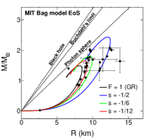
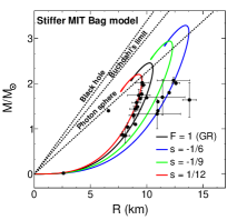
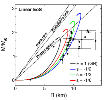
Figure 1: The variation of mass function against the radius of strange stars in the Starobinsky model for the MIT Bag model EoS (left panel), the stiffer MIT Bag model EoS (middle panel) and the linear EoS (right panel) respectively with different values of the model parameter $s$. The observational data from Table 1 are incorporated together in these plots as shown by black dots. Masses of stars are in the unit of Solar mass $\mbox{M}_{\odot}$ and the mass scale of the model $\mathcal{M}_{s}$ is taken as unity. The Buchdahl’s limit shown in this and the following two figures is the maximum compactness limit of a maximum possible massive compact stellar object in GR. This limit in MTGs should be of slightly higher value burikham .

In the second panel of Fig. 1, stars with the stiffer MIT Bag model EoS are shown. In this case it is observed that unlike the case of MIT Bag model EoS, the stiffer form is able to give the stellar structures which are capable to cross the photon sphere limit. These structures are now contributing to the emission of GW echoes. The GW echo frequency obtained for the most stable configuration with $s=-1/6$ is $59.882$ kHz. For $s=-1/9$ and $s=1/12$ the estimated echo frequencies are $63.765$ kHz and $81.829$ kHz respectively. With the positive $s$ value we have obtained larger value of echo frequency. For this case we found that, the GR case is less matching with the observational data of strange star candidates than the stellar structures obtained with the Starobinsky model. For this $f(\mathcal{R})$ model with the stiffer EoS, the most reasonable good agreement of observational data are seen for the case of $s=1/12$. Whereas the negative values of $s$ are less likely to depict the standard results for this case. Thus it can be inferred that in the case of stiffer EoS, a positive $s$ is helpful in describing the observed candidates than the negative $s$ values. Again for the stellar configurations in the Starobinsky model with the linear EoS, we observed that the stellar solutions for $s=-1/3$ is found to match pretty well with the observed strange star candidates. However, $s$ values greater than $|-1/2|$ and less than $1$ are not desirable as these values will lead to more massive compact objects ($M>3M_{\odot}$). Moreover, in this case the solutions for GR are not matching with the observed strange star candidates. Also, stars obtained from this EoS are compact enough to emit GW echo frequencies. For stars with $s=-1/2$, the characteristic echo frequency corresponding to the maximum mass configuration is found to be $55.097$ kHz. The other values of echo frequencies can be found in the Table 2.

Table 2: Physical parameters of strange stars in the Starobinsky model for different values of $s$ with $\mathcal{M}_{s}=1$.

EoSs	$s$	Radius R	Mass M	Compactness	Redshift	Echo	GWE∗	$f$-mode
		(in km)	(in $\mbox{M}_{\odot}$)	(M/R)	Z	time (ms)	frequency (kHz)	frequency (kHz)
MIT Bag model EoS	-1/2	12.101	2.437	0.298	0.600	-	-	7.580
	-1/6	9.565	1.808	0.279	0.522	-	-	11.318
	-1/12	8.875	1.651	0.275	0.503	-	-	12.656
Stiffer MIT Bag model EoS	-1/6	12.032	2.940	0.361	0.840	0.052	59.882	5.558
	-1/9	11.462	2.781	0.359	0.815	0.049	63.765	6.107
	1/12	9.293	2.204	0.351	0.752	0.038	81.829	8.646
Linear EoS	-1/2	11.097	2.793	0.372	0.679	0.057	55.097	6.206
	-1/3	10.008	2.461	0.364	0.599	0.047	66.691	7.818
	-1/6	8.831	2.124	0.356	0.544	0.039	81.158	9.897

^∗Gravitational wave echoes

In this table the maximum mass and the corresponding radius, compactness, surface redshift, characteristic echo time, echo frequency and frequency of $f$-mode of oscillation for strange stars in the Starobinsky model with three different values of the model parameter $s$ within the range allowed by observational data are listed. While calculating these values shown in the table (Table 2) and also in the Fig. 1 the mass scale of Starobinsky model is taken as $\mathcal{M}_{s}=1$, in the unit of $\mathcal{R}$. Moreover, choosing a particular value of the model parameter $s=-1/6$ and with different values of $\mathcal{M}_{s}$, all the said physical parameters related with the obtained strange star configurations are also calculated. These results are summarized in Table 3. It is observed that with the increasing values of $\mathcal{M}_{s}$, the mass, radius and compactness decreases, whereas the echo frequency increases with increase in $\mathcal{M}_{s}$ values, for all the considered cases.

Table 3: Physical parameters of strange stars in the Starobinsky model for different $\mathcal{M}_{s}$ values with $s=-1/6$.

EoSs	$\mathcal{M}^{2}_{s}$	Radius R	Mass M	Compactness	Echo	GWE
	(in units of $\mathcal{R}$)	(in km)	(in $\mbox{M}_{\odot}$)	(M/R)	time (ms)	frequency (kHz)
MIT Bag model EoS	2	8.875	1.651	0.275	-	-
	1	9.565	1.808	0.279	-	-
	2/3	10.229	1.964	0.284	-	-
Stiffer MIT Bag model EoS	2	11.171	2.701	0.358	0.047	65.866
	1	12.032	2.940	0.361	0.052	59.882
	2/3	12.854	3.175	0.365	0.057	54.690
Linear EoS	2	8.201	1.952	0.352	0.035	90.119
	1	8.831	2.124	0.356	0.039	81.158
	2/3	9.432	2.293	0.360	0.042	73.459

For the Hu-Sawicki model of $f(\mathcal{R})$ gravity the M-R profile are shown in Fig. 2. While solving this system for the Hu-Sawicki model, the mass scale value for this model is chosen to be $\mathcal{M}_{h}=1$ in the units of $\mathcal{R}$ for this particular model. The first, second and third panel of this figure correspond to the MIT Bag model EoS, stiffer MIT Bag model EoS and the linear EoS respectively. For the case of MIT Bag model EoS with three sets of model parameters $c_{1}$ and $c_{2}$, it is seen that the resulting configurations lies below the photon sphere limit and with a compactness of $\approx 0.27$. Thus these configurations cannot produce GW echoes. Incorporating Table 1 for the observed strange star candidates in these M-R profile clarifies that for the considered $c_{1}$ and $c_{2}$ values the resulting compact stars are within the observable range. As shown in the second panel of this figure, the M-R profiles given by the stiffer MIT Bag model EoS are compact enough to produce echoes. However for this typical case, the observed results are not found to match with the stars predicted by the GR case. For more negative values of $c_{1}$ and $c_{2}$, stars with larger masses and radii are found. Similar to the case of stiffer MIT Bag model EoS, the stars corresponding to linear EoSs are also ultra-compact in nature. Thus they can echo GWs falling on their stellar surfaces. In this case the observed strange star candidates are found to match with the stars given by the model parameter values $c_{1}=-0.48$, $c_{2}=-0.09$. For more smaller values of these two parameters larger configurations are obtained. A more details about the mass, radius, compactness and other physical parameters are listed in Table 4. From this table it is inferred that unlike the MIT Bag model (both softer and stiffer forms) the compactness of stellar structures increase gradually for the case of linear EoS, in the considered range of model parameter values. Also decreasing $c_{1}$ and $c_{2}$ values implies decrease in the echo frequencies of these stars. Varying the mass scale $\mathcal{M}_{h}$ also shows a mass scale dependent nature of stars. This can be seen from Table 5. From this table it is clear that for smaller $\mathcal{M}_{h}$ values the mass and radius of the most stable configuration are increasing slightly, while maintaining the constant compactness. However for the case of stiffer MIT Bag model and linear EoS, the echo frequencies decrease gradually with decrease in the $\mathcal{M}_{h}$ values.

     

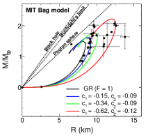
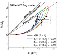
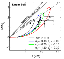
Figure 2: The variation of mass function with respect to radius of strange stars in the Hu-Sawicki model for the MIT Bag model EoS (left panel), the stiffer MIT Bag model EoS (middle panel) and the linear EoS (right panel) respectively for different values of the model parameters $c_{1}$ and $c_{2}$. The observational data from Table 1 are incorporated together in these plots as shown in black dots. Masses of stars are in the units of solar mass $M_{\odot}$ and $\mathcal{M}_{h}$ is taken as unity.

Table 4: Physical parameters of strange stars predicted by the Hu-Sawicki model for different values of the model parameters $c_{1}$ and $c_{2}$, but with $\mathcal{M}_{h}=1$.

EoSs	$c_{1}$	$c_{2}$	Radius R	Mass M	Compactness	Redshift	Echo	GWE	$f$-mode
			(in km)	(in $\mbox{M}_{\odot}$)	(M/R)	Z	time (ms)	frequency (kHz)	frequency (kHz)
MIT Bag model EoS	-0.15	-0.09	8.859	1.624	0.271	0.483	-	-	3.674
	-0.34	-0.09	9.687	1.771	0.271	0.484	-	-	3.043
	-0.62	-0.12	10.957	2.014	0.271	0.491	-	-	2.169
Stiffer MIT Bag model EoS	-0.15	-0.09	11.168	2.678	0.355	0.783	0.040	66.880	6.398
	-0.34	-0.09	12.220	2.935	0.355	0.794	0.052	60.953	5.373
	-0.48	-0.10	12.999	3.127	0.355	0.799	0.055	57.146	4.695
Linear EoS	-0.48	-0.09	9.502	2.249	0.350	0.498	0.037	79.069	8.637
	-0.70	-0.10	10.337	2.450	0.351	0.499	0.043	72.298	7.556
	-1.20	-0.30	12.426	2.988	0.355	0.546	0.054	57.705	5.268

Table 5: Physical parameters of strange stars predicted by the Hu-Sawicki model for different $\mathcal{M}_{h}$ values, but with $c_{1}=-0.15$, $c_{2}=-0.09$.

EoSs	$\mathcal{M}^{2}_{h}$	Radius R	Mass M	Compactness	Echo	GWE
	(in units of $\mathcal{R}$)	(in km)	(in $\mbox{M}_{\odot}$)	(M/R)	time (ms)	frequency (kHz)
MIT Bag model EoS	1.05	8.849	1.621	0.271	-	-
	1	8.859	1.624	0.271	-	-
	0.95	8.871	1.626	0.271	-	-
Stiffer MIT Bag model EoS	1.05	11.154	2.674	0.355	0.047	66.989
	1	11.168	2.678	0.355	0.047	66.880
	0.95	11.184	2.682	0.355	0.047	66.764
Linear EoS	1.05	8.190	1.932	0.349	0.034	92.423
	1	8.201	1.935	0.349	0.034	92.255
	0.95	8.212	1.938	0.349	0.034	92.075

For the new $f(\mathcal{R})$ gravity model i.e. for the Gogoi-Goswami model, the M-R profiles are shown in Fig. 3. In this model also the MIT Bag model EoS generally gives stars with compactness around $0.27$ and hence such compact objects cannot produce GW echoes. This is shown in the first panel of Fig. 3. For all the considered $\alpha$ and $\beta$ values, all the obtained configurations are lying below the limiting line i.e., below the photon sphere limit. In this case the stars given by the GR and for $\alpha=-0.10$, $\beta=-0.5$ are in agreement with some of the observed data of the strange star candidates. For $\alpha=-0.30$, $\beta=-3.25$, stars with configurations of maximum mass and radius are obtained, and they are laying within the observed data of similar type. For this gravity model with the MIT Bag model EoS we observed a rapid drop in compactness with smaller $\alpha$ and $\beta$ values. For the case of stiffer EoS (second panel of Fig. 3), the resulting configurations are with the compactness $>0.33$. Smaller $\alpha$ and $\beta$ values are giving larger configurations (this is applicable to all three EoSs). It is found that the combination of parameters $\alpha=0.12$ and $\beta=0.34$ represents stars with a more realistic characteristics for the stiffer EoS. For the linear EoS as shown in the third panel of Fig. 3, the solutions in GR are virtually not matching with the observed strange star candidates (in fact this is the situation for this EoS in all three figures). However, for the Gogoi-Goswami model the stellar configurations obtained with the two model parameter sets $\alpha=-0.20$, $\beta=-1.45$ and $\alpha=-0.3$, $\beta=-4.5$ are in good agreement with the observed results. These results are summarized in Table 6. As it can be visualize from the second and third panels of Fig. 3 that the resulting structures are crossing the photon sphere, so they can emit GW echo frequencies. The calculated echo frequencies are listed in Table 6. It is seen that with the decreasing $\alpha$ and $\beta$ values the echo frequencies are getting smaller for both the EoSs. Here the solutions of modified TOV equations are obtained by considering the characteristic curvature constant $\mathcal{R}_{c}=1$ when expressed in units of $\mathcal{R}$. For different $\mathcal{R}_{c}$ values the dependence on the stellar structure are shown in Table 7. It is clear from the table that when the value of $\mathcal{R}_{c}$ decreases, the characteristic echo frequency also decreases. However, the compactness of these stars are found to increase with the decrease in $\mathcal{R}_{c}$ values for all the considered EoSs.

     

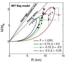
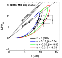
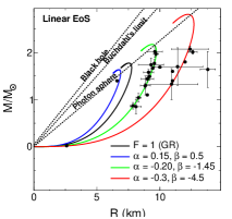
Figure 3: The variation of mass function against the radius of strange stars in the Gogoi-Goswami model for the MIT Bag model EoS (left panel), the stiffer MIT Bag model EoS (middle panel) and the linear EoS (right panel) respectively for different values of the model parameter $\alpha$ and $\beta$. The observational results from Table 1 are incorporated together in these plots as shown by black dots. Masses of stars are in the units of solar mass $M_{\odot}$ and the characteristic curvature $\mathcal{R}_{c}$ of the model is taken as unity.

Table 6: Physical parameters of strange stars predicted by the Gogoi-Goswami model for different values of the parameters $\alpha$ and $\beta$ and with $\mathcal{R}_{c}=1$.

EoSs	$\alpha$	$\beta$	Radius R	Mass M	Compactness	Redshift	Echo	GWE	$f$-mode
			(in km)	(in $\mbox{M}_{\odot}$)	(M/R)	Z	time (ms)	frequency (kHz)	frequency (kHz)
MIT Bag model EoS	0.15	0.5	7.309	1.399	0.283	0.531	-	-	4.983
	-0.10	-0.5	8.901	1.604	0.277	0.462	-	-	3.673
	-0.30	-3.25	12.074	2.124	0.260	0.438	-	-	1.490
Stiffer MIT Bag model EoS	0.12	0.34	9.492	2.306	0.359	0.817	0.041	76.804	8.394
	-0.20	-0.85	11.904	2.813	0.349	0.752	0.049	64.235	5.621
	-0.30	-1.25	12.623	2.975	0.348	0.740	0.052	60.808	4.952
Linear EoS	0.15	0.5	6.740	1.635	0.359	0.566	0.030	103.557	13.017
	-0.20	-1.45	9.382	2.172	0.342	0.434	0.037	84.853	9.210
	-0.30	-4.5	12.227	2.810	0.340	0.406	0.047	66.318	6.074

Table 7: Physical parameters of strange stars predicted by the Gogoi-Goswami model for different $\mathcal{R}_{c}$ values and with $\alpha=0.15$, $\beta=0.5$.

EoSs	$\mathcal{R}_{c}$	Radius R	Mass M	Compactness	Echo	GWE
	(in units of $\mathcal{R}$)	(in km)	(in $M_{\odot}$)	(M/R)	time (ms)	frequency (kHz)
MIT Bag model EoS	2	6.666	1.252	0.278	-	-
	1	7.309	1.399	0.283	-	-
	2/3	7.801	1.511	0.286	-	-
Stiffer MIT Bag model EoS	2	8.387	2.041	0.360	0.036	86.656
	1	9.185	2.264	0.364	0.041	76.957
	2/3	9.796	2.435	0.368	0.049	62.836
Linear EoS	2	6.157	1.474	0.354	0.025	127.571
	1	6.740	1.635	0.359	0.030	103.557
	2/3	7.187	1.758	0.362	0.032	99.597

As mentioned earlier the prime objective of the present study is to explore the astrophysical implications of the considered three well-behaved $f(\mathcal{R})$ models in the Palatini formalism in the perspectives of predictions of strange star’s behaviours. These models are considered as well-behaved models in the sense of their behaviours in the cosmological perspectives gg ; ijmpd . Thus for a better picture of the behaviours of these models in the astrophysical aspects of our study in comparison to their behaviours in the cosmological domain, we have made a comparative analysis of the ranges of parameters obtained from this study for each model with their corresponding cosmological ranges obtained from the literature, which is shown in Table 8. For the case of Starobinsky model of the form (17) with $n=1$, the constraint on the model parameter $s$ was reported earlier as $s<8/3\sqrt{3}\approx 4.618$ staro . Using the cosmic expansion and the structure growth data, the constrained value of this model parameter is reported as $s^{-1}={1.460}^{+0.47}_{-0.52}$ bessa . The viable range obtained from our study for this model’s parameter with three EoSs are shown together with the constrained range reported in Ref. staro in Table 8. From this it is clear that the range suitable for strange stars are within the cosmological limit of the model’s parameter $s$. Cosmological consequences of the Hu-Sawicki model was discussed earlier in the Ref. santos . For this gravity model a set of constraints and best-fitted values for the model parameters $c_{1}$ and $c_{2}$ were reported therein. Now the sets of the parameters $c_{1}$ and $c_{2}$ considered in this study are in the compatible range with that of the values discussed in santos . For the case of Gogoi-Goswami $f(\mathcal{R})$ gravity model a set of constrained parameters $\alpha$ and $\beta$ are discussed in gg . Keeping in mind these cosmologically constrained values we have used different sets of the model parameters which are found interesting in this study. However rather than using the positive values of this model parameters we have obtained that stellar solutions with negative values of $\alpha$ and $\beta$ are more interesting from the present perspective of the study.

Table 8: Astrophysical and cosmological ranges of the model parameters for MIT Bag model, stiffer MIT Bag model and linear EoS.

$f(\mathcal{R})$ gravity models	Model parameters	Astrophysical range from this study			Cosmological range
		MIT Bag model EoS	Stiffer MIT Bag model	Linear EoS
Starobinsky model	$s$	$-0.5$ to $-0.083$	$-0.166$ to $0.083$	$-0.5$ to $-0.167$	$<4.618$ staro
Hu-Sawicki model	$c_{1}$	$-0.62$ to $-0.15$	$-0.48$ to $-0.15$	$-1.20$ to $-0.48$	$-12.64$ to $2.23$ santos
	$c_{2}$	$-0.12$ to $-0.09$	$-0.10$ to $-0.09$	$-0.30$ to $-0.09$	$-0.85$ to $0.08$ santos
Gogoi-Goswami model	$\alpha$	$-0.30$ to $0.15$	$-0.30$ to $0.12$	$-0.30$ to $0.15$	$0.045$ to $0.300$ gg
	$\beta$	$-3.25$ to $0.5$	$-1.25$ to $0.34$	$-4.5$ to $0.5$	$0.500$ to $0.850$ gg

IV.2 Stability analysis

IV.2.1 $f$-mode of radial perturbations

In order to study the stability against radial perturbations of the compact stars in our configurations we need to calculate the fundamental $f$-mode frequencies corresponding to the radial oscillations for all those configurations. The dynamical stability against the radial adiabatic perturbation of stellar system are studied in a plethora of articles hh ; hs ; ipser ; chan ; jb . The necessary and sufficient condition for stability against radial perturbations of any physical system is that the eigenfrequency of the lowest normal mode must be real hh . In order to calculate these radial oscillation frequencies, we follow the Ref. pretel2 , where the authors considered the two-fluid formalism. Under this formalism it is considered that the star is composed of two fluids, the perfect fluid and the curvature fluid. With this idea, we can rewrite the field equation from Eq. (16) as

$$G_{\mu\nu}=8\pi(T_{\mu\nu}^{m}+T_{\mu\nu}^{c}),$$ (48)

where $T_{\mu\nu}^{m}$ is the usual matter energy-momentum tensor scaled by a factor $F_{\rho}$ as $\dfrac{T_{\mu\nu}}{F_{\rho}}$ and $T_{\mu\nu}^{c}$ is the curvature fluid with the form: $-\dfrac{\Lambda_{\rho}g_{\mu\nu}}{8\pi}$. This consideration gives us the privilege to use the standard equations of radial pulsations as discussed in Ref. pretel2 . However, one should note that these oscillation equations will result different oscillation modes as the configuration is highly dependent on the $f(\mathcal{R})$ gravity models which is followed from the modified TOV Eqs. (14)-(15).

The study of radial pulsation of stellar objects was pioneered by Chandrasekhar Chandrasekhar1964a ; Chandrasekhar1964b . The pulsation equations are coupled first order differential equation of Sturm-Liouville type and can be written as jb ; vath

$$\small{\dfrac{d\xi}{dr}=-\,\dfrac{1}{r}\left(3\xi+\dfrac{\eta}{\Gamma}\right)-\dfrac{dp}{dr}\dfrac{\xi}{p+\rho}},$$ (49)

$$\dfrac{d\eta}{dr}=\xi\left[\omega^{2}r\left(1+\dfrac{\rho}{p}\right)e^{\lambda-\chi}-\dfrac{dp}{dr}\dfrac{4}{p}-8\pi(p+\rho)\,r\,e^{\lambda}+\;\dfrac{r}{p\,(p+\rho)}{\left(\dfrac{dp}{dr}\right)}^{2}\right]+\eta\left[-\,\dfrac{\rho}{p\,(p+\rho)}\dfrac{dp}{dr}-4\pi(p+\rho)\,r\,e^{\lambda}\right],$$ (50)

where $\xi=\Delta r/r$ and $\eta=\Delta p/p$ are two dimensionless variables. $\Delta r$ is the radial perturbation and $\Delta p$ is the corresponding Lagrangian perturbations of the pressure. $\Gamma$ is the relativistic adiabatic index. It can be defined as chan

$$\Gamma=\dfrac{p+\rho}{p}\,\dfrac{dp}{d\rho}.$$ (51)

and $\omega$ is the eigenfrequency of vibration. This coupled equations are supported by two boundary conditions: at $r=0$, $\eta=-3\,\gamma\,\xi$ and $\Delta p=0$ at $r\rightarrow R_{eff}$, $R_{eff}$ is the radial distance where the total pressure goes to zero. This pulsation equations has real eigenvalues $\omega_{0}^{2}<\omega_{1}^{2}<\ldots<\omega_{n}^{2}<\ldots$, and $\omega_{n}$ are the eigenfrequencies of oscillations for $n$ nodes. The mode corresponding to $n=0$ is called the fundamental or $f$-mode. When $\omega^{2}<0$, the frequency $\omega$ becomes imaginary and it corresponds to an unstable state.

By solving these pulsation equations for all the considered cases of this study, the lowest order mode of radial oscillation i.e., $f$-mode oscillation frequencies are computed and are listed in Tables: 2, 4, 6 for Starobinsky model, Hu-Sawicki model and Gogoi-Goswami model respectively. All these frequencies are in the kHz range and are found to have real values and eventually signifies the stability of all the considered configurations.

IV.2.2 Relativistic adiabatic index

An important and necessary quantity to describe and check a region of stability of relativistic isotropic fluid sphere is the relativistic adiabatic index $\Gamma$. For the spherically symmetric spacetime with a perfect fluid Chandrasekhar Chandrasekhar1964a explored first the instability regimes using this adiabatic index. He gave a particular numerical value of the adiabatic index i.e. $\Gamma=4/3$, whose violation with higher $\Gamma$ values indicates a stable star configuration. In 1975 Heintzmann and Hillebrandt hh also proposed that isotropic compact star models are stable for $\Gamma>4/3$ throughout the stellar interior. Basically, this stability criteria was reported for the case of compact Newtonian stars bondi . Though the relativistic effects for the theory of stellar oscillations are negligible, yet for highly compact objects like neutron stars and strange stars the relativistic limits should be taken into consideration rather than the Newtonian limit. For relativistic cases the system becomes more unstable due to the regenerative effect of pressure sarkar ; erre . However, recently for a stable and relativistic dynamical system, the same condition $\Gamma>4/3$ has been considered in Refs. nashed ; biswas2 ; rej2 ; vath ; sharif ; mous ; hs .

Now to discuss the physical basis of this important stability criteria we shall briefly review stellar pulsations. The dynamic equations that govern stellar pulsations (Eqs. (49), (50)) can be written in several forms mtw ; kokkotas ; chanmugam ; vath ; godenk . Adapting the form given by Misner et al. we may write these equations as mtw

$$(P\zeta^{\prime})^{\prime}+Q\zeta+\omega^{2}W\zeta=0$$ (52)

with

$$r^{2}W=(p+\rho)e^{(3\lambda+\chi)/2},$$ (53)

$$r^{2}P=\Gamma\,p\,e^{(\lambda+3\chi)/2},$$ (54)

$$r^{2}Q=e^{(\lambda+3\chi)/2}(p+\rho)\left[(\chi^{\prime})^{2}+4\dfrac{\chi^{\prime}}{r}-8\pi e^{\lambda}p\right],$$ (55)

where the Lagrangian displacement has a harmonic time dependence as $\zeta=\zeta(r)e^{-i\omega t}$. $\zeta(r)$ and $\omega$ being the amplitude of the perturbation and the oscillation frequency, respectively.

We have boundary conditions at the origin $\zeta(r=0)=0$ and at the surface $p\,\Gamma\zeta(r)^{\prime}=0$. In both the relativistic limit and in the Newtonian limit, the oscillation problems is a Sturm-Liouville boundary value problem. In such cases the same mathematical formulations will work for both kokkotas . One method for solving such problem is the variational technique bardeen ; mtw . For a Newtonian star the pulsation equation (52) reduces to the form:

$$\left[p\,r\,\Gamma(\zeta/r)^{\prime}\right]^{\prime}+3\left(p\,\Gamma\zeta/r\right)^{\prime}-4\,p^{\prime}\zeta/r+\omega^{2}\rho\,\zeta=0.$$ (56)

For such a case the oscillation frequency can be given as

$$\omega^{2}=(3\overline{\Gamma}-4)|\Omega|/I,$$ (57)

where $I=\int{(\rho\,r^{2})\,4\,\pi r^{2}dr}$ is the trace of the second moment of the mass distribution, $\Omega$ is the star’s self-gravitational energy and $\overline{\Gamma}$ being the pressure averaged adiabatic index given as

$$\overline{\Gamma}=\dfrac{\int_{0}^{R}p\,\Gamma 4\pi r^{2}dr}{\int_{0}^{R}p\,4\pi r^{2}dr}.$$ (58)

As mentioned earlier for a physical system the necessary and sufficient condition for the stability against radial perturbations is that the eigenfrequency of the lowest normal mode must be real. From the above equation it is clear that $\overline{\Gamma}=\Gamma_{critical}=4/3$ will lead to the physically acceptable solution for the fundamental mode of oscillation. Thus for $\overline{\Gamma}>4/3$ the Newtonian star is stable in nature and will oscillate mtw . However, in the case of relativistic stars this critical value is slightly larger than $4/3$ due to relativistic effects. Hence, a sufficiently larger value of $\Gamma$ can ascertain the stability of such configurations, which is in fact already clear from the previously shown numerically calculated frequency associated to the lowest mode of oscillations.

In Figs. 4 -6 the graphical variation of relativistic adiabatic index in the stellar interior are shown for three considered $f(\mathcal{R})$ gravity models. These variations for the Starobinsky model are shown in Fig. 4. For the Starobinsky model with the MIT Bag model EoS the minimum $\Gamma$ value is obtained as $4.69$ and the variations of $\Gamma$ for $s=-1/2,-1/6,-1/12$ are shown in the first panel of Fig. 4. In the second panel of this figure, variations of $\Gamma$ are shown for the stiffer MIT Bag model and in the third panel the same are shown for the linear EoS. For the stiffer EoS the minimum $\Gamma$ value is $2.69$ and for the linear EoS it is $4.33$. As the minimum $\Gamma$ value for all these EoSs in the Starobinsky model are well above the limiting case, hence they signify the stable configurations.

     

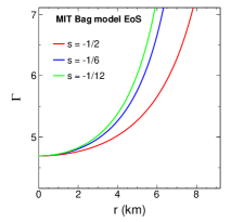
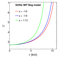
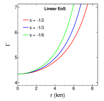
Figure 4: Behaviours of relativistic adiabatic index inside the stellar interior in the Starobinsky model for the MIT Bag model EoS (left panel), the stiffer MIT Bag model EoS (middle panel) and the linear EoS (right panel) respectively.

Fig. 5 shows the behaviour of $\Gamma$ of strange star configurations given by the Hu-Sawicki model for different considered model parameters. The central $\Gamma$ value for the stars with the MIT Bag model is $1.56$, for the stiffer MIT Bag model it is $2.69$ and for the linear EoS this value is $3.95$. Like the case in the Starobinsky model, for this model also solutions are stable against the adiabatic index.

     

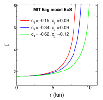
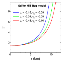
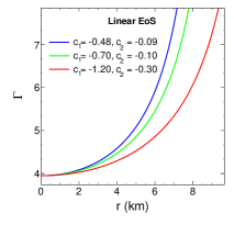
Figure 5: Behaviours of relativistic adiabatic index inside the stellar interior in the Hu-Sawicki model for the MIT Bag model EoS (left panel), the stiffer MIT Bag model EoS (middle panel) and the linear EoS (right panel) respectively.

For the case of strange stars predicted by the Gogoi-Goswami model the minimum value of $\Gamma$ obtained for the MIT Bag model, the stiffer MIT Bag model and the linear EoS are respectively $1.56$, $2.69$ and $3.95$. Variations of $\Gamma$ are shown in Fig. 6 for three EoSs respectively.

     

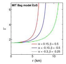
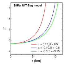
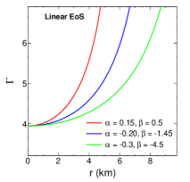
Figure 6: Behaviours of relativistic adiabatic index inside the stellar interior in the Gogoi-Goswami model for the MIT Bag model EoS (left panel), the stiffer MIT Bag model EoS (middle panel) and the linear EoS (right panel) respectively.

In all the these $f(\mathcal{R})$ gravity models and in considered EoSs, $\Gamma$ are taking values well above $4/3$ everywhere inside the stellar structure. These figures clearly ensures the non-instability regions inside the stellar structures. Fulfilment of this condition shows the stable nature of these structures.

IV.2.3 Surface redshift

The surface redshift of a star in general describes the relation between the interior geometry of the star and its EoS. As mentioned earlier we have considered the strange star configuration as isotropic, static, spherically symmetric and perfect fluid star. The compactification factor for such a star can be given as

$$u(r)=\dfrac{m(r)}{r}.$$ (59)

Using this compactification factor the surface redshift of a star can be defined as

$$Z=\dfrac{1}{\sqrt{(1-2u)}}-1$$ (60)

For isotropic stars the surface redshift $Z\leq 2$ buchdahl ; baraco . The variations of surface redshift with radial distance in the case of Starobinsky model for the three EoSs are shown in Fig. 7. The surface redshift corresponding to this $f(\mathcal{R})$ gravity model is listed in Table 2. For the MIT Bag model EoS the maximum surface redshift is $Z=0.600$. For the stiffer EoS, it is $0.840$ and for the case of linear EoS, $Z=0.679$. All these obtained redshift values are well within the desired range. For the Hu-Sawicki model the $Z$ values corresponding to each EoS with the selected sets of model parameter are given in Table 4. Also its variations can be visualized as shown in Fig. 8. The obtained maximum $Z$ values for this model are $0.491$, $0.799$ and $0.546$ for the MIT Bag model, the stiffer MIT Bag model and the linear EoS respectively. Again for the Gogoi-Goswami model the obtained results are listed in Table 6 and the variations are shown in Fig. 9. With the MIT Bag model EoS the maximum surface redshift is found as $0.531$, for the stiffer MIT Bag model it is $0.817$ and for the linear EoS this value is $0.566$. All these values are less than $2$ and hence these models predict the stable strange star configurations.

     

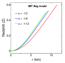
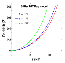
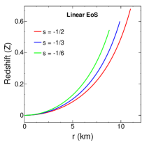
Figure 7: Behaviours of surface redshift with radial distance of strange stars in the Starobinsky model for the MIT Bag model EoS (left panel), the stiffer MIT Bag model EoS (middle panel) and the linear EoS (right panel) respectively.

     

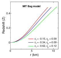
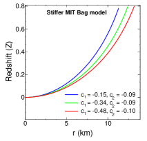
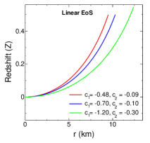
Figure 8: Behaviours of surface redshift with radial distance of strange stars in the Hu-Sawicki model for the MIT Bag model EoS (left panel), the stiffer MIT Bag model EoS (middle panel) and the linear EoS (right panel) respectively.

     

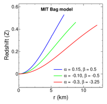
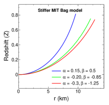
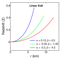
Figure 9: Behaviours of surface redshift with radial distance of strange stars in the Gogoi-Goswami model for the MIT Bag model EoS (left panel), the stiffer MIT Bag model EoS (middle panel) and the linear EoS (right panel) respectively.

V Summary and Conclusions

Strange stars in $f(\mathcal{R})$ gravity Palatini formalism have been studied in Ref. panotopoulos , where the author used the MIT Bag model EoS to study the respective stellar structures. But in this work, we have extended the study to three EoSs viz., MIT Bag model, stiffer MIT Bag model and linear EoSs for three different viable and well-established dark energy $f(\mathcal{R})$ gravity models. It is worth mentioning that strange stars were not studied earlier using the later two EoSs in the $f(\mathcal{R})$ Palatini formalism. For the later two EoSs, the trace of the energy-momentum tensor becomes the density dependent resulting a complex situation. We have solved the corresponding TOV equations numerically and obtained the stellar structures for the three different $f(\mathcal{R})$ gravity models using different model parameters within their most reliable ranges. Because we have chosen the model parameters in compliance with the most promising candidates of strange stars obtained so far. The results show that the $f(\mathcal{R})$ gravity models support the possibilities of such stable strange stars. Moreover, we have also shown that the linear and the stiffer MIT Bag model EoSs provide the possible strange stars that can echo the GWs. For the Starobinsky model with the stiffer EoS, we have seen that the M-R curve for $s=1/12$ shows good agreement with most of the observed strange star candidates. For this case, the GW echo frequency is found to be $81.829$ kHz with echo time $0.038$ ms. On the other hand, for the linear EoS, $s=-1/3$ shows a better agreement with the experimentally obtained strange star candidates. The corresponding echo frequency is found to be $66.691$ kHz with an echo time $0.047$ ms. For the later EoS, we observe a decrease in the echo frequency and increase in the echo time. For the Hu-Sawicki model with the stiffer EoS, we can see that the model shows a significant deviation from the experimental results and the M-R curves are not found in a good agreement with the experimental candidates in the GR limit also. On the other hand, for the linear EoS with $c_{1}=-0.48$ and $c_{2}=-0.09$, the M-R curve covers most of the experimental candidates with a possibility of GW echo frequency $79.069$ kHz with echo time $0.037$ ms. Finally, we considered the Gogoi-Goswami model, in which the stiffer MIT Bag model, with $\alpha=0.12$ and $\beta=0.34$ shows a better agreement with the observed strange star candidates along with a possibility of GW echo frequency $76.804$ kHz and echo time $0.041$ ms. While for the linear EoS case, the M-R curve of $\alpha=-0.20$ and $\beta=-1.45$ shows a good agreement with the observed candidates with an echo frequency $84.853$ kHz and echo time $0.037$ ms.

These predicted echo frequencies of GWs will get their firm footing once they are detected experimentally. The echo frequencies that we have estimated for all the considered cases lay above $50$ kHz. So far GWs with frequencies of $\sim 20$ Hz - $4$ kHz and with amplitudes of $\sim 2\times 10^{-22}$ - $4\times 10^{-24}$ strain/$\sqrt{\mbox{Hz}}$ martynov ; abbot are projected at GW detectors like, Advanced LIGO ligo , Advanced Virgo virgo and KAGRA kagra . Currently running LIGO currentligo and Virgo currentvirgo observatories have a sensitivity of $\geq 2\times 10^{-23}$ strain/$\sqrt{\mbox{Hz}}$ at $3$ kHz. The third generation detectors, such as Cosmic Explorer (CE) abbott and Einstein Telescope (ET) punturo with optimal arm length of $\approx 20$ km would have the sensitivity to detect the amount of postmerger neutron star oscillations punturo . The sensitivity of CE may reach below $10^{-25}$ strain/$\sqrt{\mbox{Hz}}$ at above few kHz frequencies and it is a proposed $40$ km arm length L-shaped observatory. On the other hand, ET - the L-shaped underground proposed observatory will be able to reach the sensitivity of $>3\times 10^{-25}$ strain/$\sqrt{\mbox{Hz}}$ at $100$ Hz and of $\sim 6\times 10^{-24}$ strain/$\sqrt{\mbox{Hz}}$ at $\sim 10$ kHz. Thus, the present and near future GW detectors are not enough sensitive to detect such weak signals of GWs. However, the enhancement of the sensitivity of these detectors are also possible. It is proposed that the sensitivity of these detectors can be enhanced by an optical configuration of detectors using the current interferometer topology to reach $\geq 7\times 10^{-25}$ strain/$\sqrt{\mbox{Hz}}$ at $2.5$ kHz martynov . Also, S. L. Danilishin et al. danilishin proposed that by the application of advanced quantum techniques to suppress the quantum noise at high frequency end in the design of GW detectors, the sensitivity of the present GW detectors can be enhanced significantly. If applications of such techniques or other possible method can enhance the sensitivity of GW detectors, it will open a new door to explore such echoes of the GWs. Which will definitely throw more light on the mystery of stellar interior of compact stars.

An important point to be noted here is that the $f(\mathcal{R})$ gravity models considered in this study are the dark energy $f(\mathcal{R})$ gravity models, which can mimic the $\Lambda$CDM model at high curvature regime and GR in the low curvature regime. The general Starobinsky model also behaves in the similar manner but the special case we have considered in this work is the inflationary Starobinsky model which is well known for its capabilities of explaining the theoretical inflationary epoch of the universe. On the other hand, the Gogoi-Goswami model and the Hu-Sawicki model show very promising behaviour in the cosmological perspectives and both the models, in Palatini formalism can explain the present universe and far past scenario of the universe effectively ijmpd . At far past or very high redshift range both the models are identical to the $\Lambda$CDM model, which makes it almost difficult to differentiate the models in high curvature regime. But our studies showed that the compact star structure at very high curvature has a high model dependency which provides us a new avenue in constraining the models in high curvature regime. So, undoubtedly studies of such modified gravity models in the area of compact stars will provide a better constraint on the model parameters in the high curvature regime once we have a good number of experimental results in this direction.

From these results, we can conclude that the $f(\mathcal{R})$ gravity in Palatini formalism allows the formation of stable strange stars, and can explain the stability and existence of the experimentally obtained strange star candidates. Nevertheless, to have a clear picture of the stability of such stellar configurations, a more detailed analysis throughout the complete model parameter space would be necessary. As this sort of study would be beyond the scope of the present one, so we leave this as a future prospect of the study. We have also provided the echo frequencies and times for such compact structures. In the near future, with the experimental data of GW echoes from such candidates it might be possible to select the most promising EoS or constraining the EoSs, which will provide a better understanding of such configurations and hence will help to reveal the actual properties of such stars. Consequently, the physics of near and the high regime will be solved clearly afterwards.

References

- (1) D. N. Spergel et. al., Three‐Year Wilkinson Microwave Anisotropy Probe ( WMAP ) Observations: Implications for Cosmology, Astrophys. J Suppl. S 170, 377 (2007).
- (2) P. Astier et. al., The Supernova Legacy Survey: Measurement of , and from the First Year Data Set, A&A 447, 31 (2006).
- (3) P. D. Naselskii and A. G. Polnarev, Candidate Missing Mass Carriers in an Inflationary Universe, Soviet Astronomy 29, 487 (1985).
- (4) A. G. Riess et. al., Observational Evidence from Supernovae for an Accelerating Universe and a Cosmological Constant, ApJ 116, 1009 (1998).
- (5) S. Perlmutter et. al., Measurements of and from 42 High‐Redshift Supernovae, ApJ 517, 565 (1999).
- (6) S. Capozziello and V. Faraoni, Beyond Einstein Gravity: A Survey of Gravitational Theories for Cosmology and Astrophysics (Springer, New York, 2011).
- (7) G. Bertone and D. Hooper, History of Dark Matter, Rev. Mod. Phys. 90, 045002 (2018).
- (8) C. Bohmer, T. Harko, and F. Lobo, Dark Matter as a Geometric Effect in f(R) Gravity, Astropart. Phys. 29, 386 (2008).
- (9) N. Parbin and U. D. Goswami, Scalarons mimicking dark matter in the Hu-Sawicki model of gravity, Mod. Phys. Lett. A 36, 2150265 (2021).
- (10) T. Harko and F. S. N. Lobo, Extensions of f(R) Gravity: Curvature-Matter Couplings and Hybrid Metric-Palatini Gravity (Cambridge University Press, Cambridge, 2018).
- (11) S. Nojiri and S. D. Odintsov, Unified Cosmic History in Modified Gravity: From Theory to Lorentz Non-Invariant Models, Physics Reports 505, 59 (2011).
- (12) S. Nojiri, S. D. Odintsov, and V. K. Oikonomou, Modified Gravity Theories on a Nutshell: Inflation, Bounce and Late-Time Evolution, Physics Reports 692, 1 (2017).
- (13) T. Clifton, P. G. Ferreira, A. Padilla, and C. Skordis, Modified Gravity and Cosmology, Physics Reports 513, 1 (2012).
- (14) N. K. Glendenning, Compact Stars: Nuclear Physics, Particle Physics, and General Relativity, 2nd ed (Springer, New York, 2000).
- (15) S. L. Shapiro and S. A. Teukolsky, Black Holes, White Dwarfs, and Neutron Stars: The Physics of Compact Objects, 1st ed. (Wiley, 1983).
- (16) C. Alcock, E. Farhi, and A. Olinto, Strange Stars, ApJ 310, 261 (1986).
- (17) M. Alford, M. Braby, M. Paris, and S. Reddy, Hybrid Stars That Masquerade as Neutron Stars, ApJ 629, 969 (2005).
- (18) M. Visser and D. L. Wiltshire, Stable Gravastars—an Alternative to Black Holes?, Class. Quantum Grav. 21, 1135 (2004).
- (19) P. Jetzer, Boson Stars, Physics Reports 220, 163 (1992).
- (20) E. Braaten, A. Mohapatra, and H. Zhang, Dense Axion Stars, Phys. Rev. Lett. 117, 121801 (2016).
- (21) D.-C. Dai, A. Lue, G. Starkman, and D. Stojkovic, Electroweak Stars: How Nature May Capitalize on the Standard Model’s Ultimate Fuel, J. Cosmol. Astropart. Phys. 12, 004 (2010).
- (22) E. Farhi and R. L. Jaffe, Strange Matter, Phys. Rev. D 30, 2379 (1984).
- (23) E. Witten, Cosmic Separation of Phases, Phys. Rev. D 30, 272 (1984).
- (24) G. Baym and S. A. Chin, Can a Neutron Star Be a Giant MIT Bag?, Phys. Lett. B 62, 241 (1976).
- (25) C. Alcock and A. Olinto, Exotic Phases of Hadronic Matter and Their Astrophysical Application, Annu. Rev. Nucl. Part. Sci. 38, 161 (1988).
- (26) P. Haensel, J. L. Zdunik, and R. Schaefer, Strange Quark Stars, A&A 160, 121 (1986).
- (27) E. O. Ofek et. al., SN 2006gy: An Extremely Luminous Supernova in the Galaxy NGC 1260, ApJ 659, L13 (2007).
- (28) R. Ouyed, D. Leahy, and P. Jaikumar, Predictions for Signatures of the Quark-Nova in Superluminous Supernovae, arXiv:0911.5424v1 (2009).
- (29) T. Overgard and E. Ostgaard, Mass, Radius, and Moment of Inertia for Hypothetical Quark Stars., A&A 243, 412 (1991).
- (30) I. Lopes, G. Panotopoulos, and Á. Rincón, Anisotropic Strange Quark Stars with a Non-Linear Equation-of-State, Eur. Phys. J. Plus 134, 454 (2019).
- (31) S. K. Maurya and F. Tello-Ortiz, Charged Anisotropic Strange Stars in General Relativity, Eur. Phys. J. C 79, 33 (2019).
- (32) J. Bora and U. Dev Goswami, Radial Oscillations and Gravitational Wave Echoes of Strange Stars with Nonvanishing Lambda, Astropart. Phys. 143, 102744 (2022).
- (33) S. K. Maurya, A. Errehymy, D. Deb, F. Tello-Ortiz, and M. Daoud, Study of Anisotropic Strange Stars in f(R,T) Gravity: An Embedding Approach under the Simplest Linear Functional of the Matter-Geometry Coupling, Phys. Rev. D 100, 044014 (2019).
- (34) G. Panotopoulos and Á. Rincón, Relativistic Strange Quark Stars in Lovelock Gravity, Eur. Phys. J. Plus 134, 472 (2019).
- (35) K. V. Staykov, D. D. Doneva, S. S. Yazadjiev, and K. D. Kokkotas, Slowly Rotating Neutron and Strange Stars in Gravity, J. Cosmol. Astropart. Phys. 10, 006 (2014).
- (36) D. Deb, F. Rahaman, S. Ray, and B. K. Guha, Strange Stars in Gravity, J. Cosmol. Astropart. Phys. 03, 044 (2018).
- (37) J. M. Z. Pretel, S. E. Jorás, R. R. R. Reis, and J. D. V. Arbañil, Radial Oscillations and Stability of Compact Stars in f(R,T)= R+2T Gravity, J. Cosmol. Astropart. Phys. 04, 064 (2021).
- (38) P. Bhar, Charged Strange Star with Krori-Barua Potential in f(R,T) Gravity Admitting Chaplygin Equation of State, Eur. Phys. J. Plus 135, 757 (2020).
- (39) S. Biswas, D. Shee, B. K. Guha, and S. Ray, Anisotropic Strange Star with Tolman-Kuchowicz Metric under f(R,T) Gravity, Eur. Phys. J. C 80, 175 (2020).
- (40) P. Rej and P. Bhar, Charged Strange Star in Gravity with Linear Equation of State, Astrophys. Space Sci. 366, 35 (2021).
- (41) S. H. Hendi, G. H. Bordbar, B. E. Panah, and S. Panahiyan, Modified TOV in Gravity’s Rainbow: Properties of Neutron Stars and Dynamical Stability Conditions, J. Cosmol. Astropart. Phys. 09, 013 (2016).
- (42) B. Eslam Panah and H. L. Liu, White Dwarfs in de Rham-Gabadadze-Tolley like Massive Gravity, Phys. Rev. D 99, 104074 (2019).
- (43) A. V. Astashenok, S. Capozziello, S. D. Odintsov, and V. K. Oikonomou, Causal Limit of Neutron Star Maximum Mass in f(R) Gravity in View of GW190814, Phys. Lett. B 816, 136222 (2021).
- (44) G. J. Olmo, Post-Newtonian Constraints on f(R) Cosmologies in Metric and Palatini Formalism, Phys. Rev. D 72, 083505 (2005).
- (45) G. J. Olmo and D. Rubiera-Garcia, Junction Conditions in Palatini f(R) Gravity, Class. Quantum Grav. 37, 215002 (2020).
- (46) G. J. Olmo and D. Rubiera-Garcia, Palatini f(R) Black Holes in Nonlinear Electrodynamics, Phys. Rev. D 84, 124059 (2011).
- (47) G. J. Olmo and D. Rubiera-Garcia, Reissner-Nordström Black Holes in Extended Palatini Theories, Phys. Rev. D 86, 044014 (2012).
- (48) C. Bejarano, G. J. Olmo, and D. Rubiera-Garcia, What Is a Singular Black Hole beyond General Relativity?, Phys. Rev. D 95, 064043 (2017).
- (49) C. Bambi, A. Cardenas-Avendano, G. J. Olmo, and D. Rubiera-Garcia, Wormholes and Nonsingular Spacetimes in Palatini f(R) Gravity, Phys. Rev. D 93, 064016 (2016).
- (50) G. J. Olmo, D. Rubiera-Garcia, and A. Sanchez-Puente, Classical Resolution of Black Hole Singularities via Wormholes, Eur. Phys. J. C 76, 143 (2016).
- (51) G. J. Olmo, D. Rubiera-Garcia, and A. Wojnar, Minimum Main Sequence Mass in Quadratic Palatini f(R) Gravity, Phys. Rev. D 100, 044020 (2019).
- (52) K. Kainulainen, V. Reijonen, and D. Sunhede, Interior Spacetimes of Stars in Palatini Gravity, Phys. Rev. D 76, 043503 (2007).
- (53) G. Panotopoulos, Strange Stars in f(R) Theories of Gravity in the Palatini Formalism, Gen. Relativ. Gravit. 49, 69 (2017).
- (54) R. Goswami, S. D. Maharaj, and A. M. Nzioki, Buchdahl-Bondi Limit in Modified Gravity: Packing Extra Effective Mass in Relativistic Compact Stars, Phys. Rev. D 92, 064002 (2015).
- (55) E. Berti et al., Testing General Relativity with Present and Future Astrophysical Observations, Class. Quantum Grav. 32, 243001 (2015).
- (56) M. Z. Bhatti, Z. Yousaf, and Zarnoor, Stability of Charged Neutron Star in Palatini f(R) Gravity, Mod. Phys. Lett. A 34, 1950252 (2019).
- (57) G. J. Olmo, D. Rubiera-Garcia, and A. Wojnar, Stellar Structure Models in Modified Theories of Gravity: Lessons and Challenges, Physics Reports 876, 1 (2020).
- (58) D. J. Nice, E. M. Splaver, I. H. Stairs, O. Lohmer, A. Jessner, M. Kramer, and J. M. Cordes, A 2.1 M⊙ Pulsar Measured by Relativistic Orbital Decay, ApJ 634, 1242 (2005).
- (59) M. H. van Kerkwijk, R. P. Breton, and S. R. Kulkarni, Evidence for a massive neutron star from a radial-velocity study of the companion to the black-widow pulsar PSR B1957+20, ApJ 728, 95 (2011).
- (60) C. E. Rhoades and R. Ruffini, Maximum Mass of a Neutron Star, Phys. Rev. Lett. 32, 324 (1974).
- (61) V. Kalogera and G. Baym, The Maximum Mass of a Neutron Star, ApJ 470, L61 (1996).
- (62) J. Alsing, H. O. Silva, and E. Berti, Evidence for a Maximum Mass Cut-off in the Neutron Star Mass Distribution and Constraints on the Equation of State, Monthly Notices of the Royal Astronomical Society 478, 1377 (2018).
- (63) R. Konoplya and A. Zhidenko, Detection of Gravitational Waves from Black Holes: Is There a Window for Alternative Theories?, Physics Letters B 756, 350 (2016).
- (64) J. Vainio and I. Vilja, F(R) Gravity Constraints from Gravitational Waves, Gen. Relativ. Gravit. 49, 99 (2017).
- (65) H. Grigorian, D. N. Voskresensky and D. Blaschke, Influence of the stiffness of the equation of state and in-medium effects on the cooling of compact stars, The Eur. Phys. J. A 52, 67 (2016).
- (66) C. H. Lenzi and G. Lugones, Hybrid Stars in the Light of the Massive Pulsar PSR J1614–2230, ApJ 759, 57 (2012).
- (67) A. Li, F. Huang and R.-X. Xu, Too massive neutron stars: The role of dark matter?, Astropart. Phys. 37, 70 (2012).
- (68) D. Psaltis, Probes and Tests of Strong-Field Gravity with Observations in the Electromagnetic Spectrum, Living Rev. Relativ. 11, 9 (2008).
- (69) G. J. Olmo, Reexamination of Polytropic Spheres in Palatini Gravity, Phys. Rev. D 78, 104026 (2008).
- (70) F. A. Teppa Pannia, F. García, S. E. Perez Bergliaffa, M. Orellana, and G. E. Romero, Structure of Compact Stars in R-Squared Palatini Gravity, Gen. Relativ. Gravit. 49, 25 (2017).
- (71) F. A. Silveira, R. Maier, and S. E. Perez Bergliaffa, A Model of Compact and Ultracompact Objects in -Palatini Theory, Eur. Phys. J. C 81, 7 (2021).
- (72) J. Bora and U. D. Goswami, Radial Oscillations and Gravitational Wave Echoes of Strange Stars for Various Equations of State, Monthly Notices of the Royal Astronomical Society 502, 1557 (2021).
- (73) P. Pani and V. Ferrari, On Gravitational-Wave Echoes from Neutron-Star Binary Coalescences, Class. Quantum Grav. 35, 15LT01 (2018).
- (74) M. Mannarelli and F. Tonelli, Gravitational Wave Echoes from Strange Stars, Phys. Rev. D 97, 123010 (2018).
- (75) A. Urbano and H. Veerm ae, On Gravitational Echoes from Ultracompact Exotic Stars, J. Cosmol. Astropart. Phys. 04, 011 (2019).
- (76) C. Zhang, Gravitational Wave Echoes from Interacting Quark Stars, Phys. Rev. D 104, 083032 (2021).
- (77) A. A. Starobinsky, A New Type of Isotropic Cosmological Models without Singularity, Phys. Lett. B 91, 99 (1980).
- (78) W. Hu and I. Sawicki, Models of f(R) Cosmic Acceleration That Evade Solar System Tests, Phys. Rev. D 76, 064004 (2007).
- (79) D. J. Gogoi and U. D. Goswami, A New f(R) Gravity Model and Properties of Gravitational Waves in It, Eur. Phys. J. C 80, 1101 (2020).
- (80) R. C. Tolman, Static Solutions of Einstein’s Field Equations for Spheres of Fluid, Phys. Rev. 55, 364 (1939).
- (81) J. R. Oppenheimer and G. M. Volkoff, On Massive Neutron Cores, Phys. Rev. 55, 374 (1939).
- (82) A. Chodos, R. L. Jaffe, K. Johnson, C. B. Thorn, and V. F. Weisskopf, New Extended Model of Hadrons, Phys. Rev. D 9, 3471 (1974).
- (83) A. Chodos, R. L. Jaffe, K. Johnson, and C. B. Thorn, Baryon Structure in the Bag Theory, Phys. Rev. D 10, 2599 (1974).
- (84) A. Aziz, S. Ray, F. Rahaman, M. Khlopov, and B. K. Guha, Constraining Values of Bag Constant for Strange Star Candidates, Int. J. Mod. Phys. D 28, 1941006 (2019).
- (85) M. Dey, I. Bombaci, J. Dey, S. Ray, and B. C. Samanta, Strange Stars with Realistic Quark Vector Interaction and Phenomenological Density-Dependent Scalar Potential, Phys. Lett. B 438, 123 (1998).
- (86) W. Israel, Singular Hypersurfaces and Thin Shells in General Relativity, Nuov. Cim. B 44, 1 (1966).
- (87) G. Darmois, The equations of Einsteinian gravitation Mathematical Sciences Memorial, no. 25 , 58 (1927).
- (88) M. Sharif and A. Majid, Anisotropic Strange Stars through Embedding Technique in Massive Brans–Dicke Gravity, Eur. Phys. J. Plus 135, 558 (2020).
- (89) O. Sokoliuk, A. Baransky, and P. K. Sahoo, Non-Singular T-K Axion Stars with/without the Dynamical Bosonic Field in the Presence of Negative Term, Phys. Dark Univ. 35, 100972 (2022).
- (90) C.-M. Claudel, K. S. Virbhadra, and G. F. R. Ellis, The Geometry of Photon Surfaces, J. Math. Phys. 42, 818 (2001).
- (91) H. A. Buchdahl, General Relativistic Fluid Spheres, Phys. Rev. 116, 1027 (1959).
- (92) P. Burikham, T. Harko, and M. J. Lake, Mass Bounds for Compact Spherically Symmetric Objects in Generalized Gravity Theories, Phys. Rev. D 94, 064070 (2016).
- (93) H. T. Cromartie et. al., Relativistic Shapiro Delay Measurements of an Extremely Massive Millisecond Pulsar, Nat. Astron. 4, 72 (2020).
- (94) P. Kaaret, E. C. Ford, and K. Chen, Strong-Field General Relativity and Quasi-Periodic Oscillations in X-Ray Binaries, ApJ 480, L27 (1997).
- (95) J. Antoniadis et. al., A Massive Pulsar in a Compact Relativistic Binary, Science 340, 1233232 (2013).
- (96) P. B. Demorest, T. Pennucci, S. M. Ransom, M. S. E. Roberts, and J. W. T. Hessels, A Two-Solar-Mass Neutron Star Measured Using Shapiro Delay, Nature 467, 1081 (2010).
- (97) T. Gangopadhyay, S. Ray, X.-D. Li, J. Dey, and M. Dey, Strange Star Equation of State Fits the Refined Mass Measurement of 12 Pulsars and Predicts Their Radii, Monthly Notices of the Royal Astronomical Society 431, 3216 (2013).
- (98) M. K. Abubekerov, E. A. Antokhina, A. M. Cherepashchuk, and V. V. Shimanskii, The Mass of the Compact Object in the X-Ray Binary Her X-1/HZ Her, Astron. Rep. 52, 379 (2008).
- (99) M. L. Rawls, J. A. Orosz, J. E. McClintock, M. A. P. Torres, C. D. Bailyn, and M. M. Buxton, Refined Neutron Star Mass Determinations for Six Eclipsing X-ray Pulsar Binaries, ApJ 730, 25 (2011).
- (100) J. Poutanen and M. Gierlinski, On the Nature of the X-Ray Emission from the Accreting Millisecond Pulsar SAX J1808.4-3658, Monthly Notices of the Royal Astronomical Society 343, 1301 (2003).
- (101) J. J. Drake et. al., Is RX J1856.5-3754 a Quark Star?, ApJ 572, 996 (2002).
- (102) R. Iaria et. al., A Possible Cyclotron Resonance Scattering Feature near 0.7 KeV in X1822-371, A&A 577, A63 (2015).
- (103) P. C. C. Freire et. al., On the Nature and Evolution of the Unique Binary Pulsar J1903+0327: PSR J1903+0327, Monthly Notices of the Royal Astronomical Society 412, 2763 (2011).
- (104) N. Degenaar et. al., Probing the Crust of the Neutron Star in EXO 0748-676, ApJ 791, 47 (2014).
- (105) X.-D. Li, I. Bombaci, M. Dey, J. Dey, and E. P. J. van den Heuvel, Is SAX J1808.4-3658 a Strange Star?, Phys. Rev. Lett. 83, 3776 (1999).
- (106) T. Güver, P. Wroblewski, arXiv:2112.00822 L. Camarota, and F. Özel, The Mass and Radius of the Neutron Star in 4U 1820–30, ApJ 719, 1807 (2010).
- (107) L. Titarchuk and N. Shaposhnikov, Three Type I X-Ray Bursts from Cygnus X-2: Application of Analytical Models for Neutron Star Mass and Radius Determination, ApJ 570, L25 (2002).
- (108) X. Ren-Xin, X. Xuan-Bin, and W. Xin-Ji, The Fastest Rotating Pulsar: A Strange Star?, Chinese Phys. Lett. 18, 837 (2001).
- (109) F. Özel, T. Güver, and D. Psaltis, The Mass And Radius of the Neutron Star in EXO 1745–248, ApJ 693, 1775 (2009).
- (110) T. Güver and F. Özel, The Mass And Radius of the Neutron Star in the Transiant Low-Mass X-Ray Binary SAX J1748.9–2021, ApJ 765, L1 (2013).
- (111) X.-D. Li, S. Ray, J. Dey, M. Dey, and I. Bombaci, On the Nature of the Compact Star in 4U 1728-34, ApJ 527, L51 (1999).
- (112) A. K. F. Val Baker, A. J. Norton, and H. Quaintrell, The Mass of the Neutron Star in SMC X-1, A&A 441, 685 (2005).
- (113) Y. L. Yue, X. H. Cui, and R. X. Xu, Is PSR B0943+10 a Low-Mass Quark Star?, ApJ 649, L95 (2006).
- (114) D. J. Gogoi and U. D. Goswami, Cosmology with a new f(R) gravity model in Palatini formalism, Int. J. Mod. Phys. D. 31, 2250048 (2022).
- (115) P. Bessa, M. Campista, and A. Bernui, Observational Constraints on Starobinsky Cosmology from Cosmic Expansion and Structure Growth Data, Eur. Phys. J. C 82, 506 (2022).
- (116) B. Santos, M. Campista, J. Santos, and J. S. Alcaniz, Cosmology with Hu-Sawicki Gravity in the Palatini Formalism, A&A 548, A31 (2012).
- (117) H. Heintzmann and W. Hillebrandt, Neutron Stars with an Anisotropic Equation of State: Mass, Redshift and Stability., A&A 38, 51 (1975).
- (118) W. Hillebrandt and K. O. Steinmetz, Anisotropic Neutron Star Models: Stability against Radial and Nonradial Pulsations, A&A 53, 283 (1976).
- (119) R. Chan, L. Herrera, and N. O. Santos, Dynamical Instability for Radiating Anisotropic Collapse, Monthly Notices of the Royal Astronomical Society 265, 533 (1993).
- (120) J. R. Ipser, On the Stability of Ultrarelativistic Stars, Astrophys. Space Sci. 7, 361 (1970).
- (121) J. M. Z. Pretel, S. E. Jorás, and R. R. R. Reis, Strongest Constraint in Gravity: Stellar Stability, J. Cosmol. Astropart. Phys. 11, 048 (2020).
- (122) S. Chandrasekhar, The Dynamical Instability of Gaseous Masses Approaching the Schwarzschild Limit in General Relativity., ApJ 140, 417 (1964).
- (123) S. Chandrasekhar, Dynamical Instability of Gaseous Masses Approaching the Schwarzschild Limit in General Relativity, Phys. Rev. Lett. 12, 114 (1964).
- (124) H. M. Väth and G. Chanmugam, Radial Oscillations of Neutron Stars and Strange Stars, A&A 260, 250 (1992).
- (125) H. Bondi, The Contraction of Gravitating Spheres, Proc. R. Soc. Lond. A 281, 39 (1964).
- (126) N. Sarkar, S. Sarkar, Ksh. N. Singh, and F. Rahaman, Relativistic Compact Stars with Dark Matter Density Profile, Eur. Phys. J. C 80, 255 (2020).
- (127) A. Errehymy, Y. Khedif, and M. Daoud, Anisotropic Compact Stars via Embedding Approach in General Relativity: New Physical Insights of Stellar Configurations, Eur. Phys. J. C 81, 266 (2021).
- (128) G. G. L. Nashed and S. Capozziello, Anisotropic Compact Stars in f(R) Gravity, Eur. Phys. J. C 81, 481 (2021).
- (129) S. Biswas, D. Deb, S. Ray, and B. K. Guha, Anisotropic Charged Strange Stars in Krori-Barua Spacetime under f(R,T) Gravity, Ann. Phys. 428, 168429 (2021).
- (130) P. Rej and P. Bhar, Charged Strange Star in Gravity with Linear Equation of State, Astrophys. Space Sci. 366, 35 (2021).
- (131) M. Sharif and A. Waseem, Anisotropic Quark Stars in f(R,T) Gravity, Eur. Phys. J. C 78, 868 (2018).
- (132) Ch. C. Moustakidis, The Stability of Relativistic Stars and the Role of the Adiabatic Index, Gen. Relativ. Gravit. 49, 68 (2017).
- (133) C. W. Misner, K. S. Thorne, and J. A. Wheeler, Gravitation (W. H. Freeman, San Francisco, 1973).
- (134) K. D. Kokkotas and J. Ruoff, Radial Oscillations of Relativistic Stars, A&A 366, 565 (2001).
- (135) G. Chanmugam, Radial Oscillations of Zero-Temperature White Dwarfs and Neutron Stars below Nuclear Densities, ApJ 217, 799 (1977).
- (136) D. Gondek, P. Haensel, and J. L. Zdunik, Radial Pulsations and Stability of Protoneutron Stars, A&A 325, 217 (1997).
- (137) J. M. Bardeen, K. S. Thorne, and D. W. Meltzer, A Catalogue of Methods for Studying the Normal Modes of Radial Pulsation of General-Relativistic Stellar Models, ApJ 145, 505 (1966).
- (138) D. Barraco and V. H. Hamity, Maximum Mass of a Spherically Symmetric Isotropic Star, Phys. Rev. D 65, 124028 (2002).
- (139) D. Martynov et al., Exploring the Sensitivity of Gravitational Wave Detectors to Neutron Star Physics, Phys. Rev. D 99, 102004 (2019).
- (140) B. Abbott et al., Prospects for Observing and Localizing Gravitational-Wave Transients with Advanced LIGO, Advanced Virgo and KAGRA, Living Rev. Relativ. 23, 3 (2020).
- (141) J. Aasi et al., Advanced LIGO, Class. Quantum Grav. 32, 074001 (2015).
- (142) F. Acernese et al., Advanced Virgo: A Second-Generation Interferometric Gravitational Wave Detector, Class. Quantum Grav. 32, 024001 (2015).
- (143) Y. Aso, Y. Michimura, K. Somiya, M. Ando, O. Miyakawa, T. Sekiguchi, D. Tatsumi, and H. Yamamoto, Interferometer Design of the KAGRA Gravitational Wave Detector, Phys. Rev. D 88, 043007 (2013).
- (144) B. P. Abbott et al., LIGO: The Laser Interferometer Gravitational-Wave Observatory, Rep. Prog. Phys. 72, 076901 (2009).
- (145) B. Caron et al., The Virgo interferometer, Class. Quantum Grav. 14, 1461 (1997).
- (146) B. Abbott et al., GW170817: Observation of Gravitational Waves from a Binary Neutron Star Inspiral, Phys. Rev. Lett. 119, 161101 (2017).
- (147) M. Punturo et al., The Einstein Telescope: A Third-Generation Gravitational Wave Observatory, Class. Quantum Grav. 27, 194002 (2010).
- (148) S. L. Danilishin, F. Y. Khalili , H. Miao, Advanced Quantum Techniques for Future Gravitational-Wave Detectors, Living Rev. Relativ. 22, 2 (2019).