GPU PARALLEL ALGORITHM FOR THE GENERATION OF POLYGONAL MESHES BASED ON TERMINAL-EDGE REGIONS

GPU PARALLEL ALGORITHM FOR THE GENERATION OF POLYGONAL MESHES BASED ON TERMINAL-EDGE REGIONS

Abstract

This paper presents a GPU parallel algorithm to generate a new kind of polygonal meshes obtained from Delaunay triangulations. To generate the polygonal mesh, the algorithm first uses a classification system to label each edge of an input triangulation; second it builds polygons (simple or not) from terminal-edge regions using the label system, and third it transforms each non-simple polygon from the previous phase into simple ones, convex or not convex polygons. We show some preliminary experiments to test the scalability of the algorithm and compare it with the sequential version. We also run a very simple test to show that these meshes can be useful for the virtual element method.

1 Introduction

Polygonal mesh generation is an area of study broadly researched due to their applications in computer graphics [1], geographic information systems [2] and finite element methods (FEM) [3], among others. As a result of the FEM research, several requirements on the shape of the basic cells have been established as quality shape criteria. Typical meshes tend to contain only triangles or quadrilaterals; the big exception is the use of Voronoi regions (convex polygons) as basic cells [4]. However, in the recent years, the virtual element method (VEM) [5] has showed to work with polygons convex and non convex [6, 7], so a new area of study to generate quality meshes for the VEM has begun [8, 9].

Common methods to generate unstructured mesh generation are the Delaunay methods [10], Voronoi diagram methods [11, 12, 13], Advancing front method [14], quadtree based methods [15] and hybrids methods [16]. In general, meshing algorithms can be classified into two groups [17, 18]: (i) direct algorithms: meshes are generated from the input geometry, and (ii) indirect algorithms: meshes are generated starting from an input mesh, tipically an initial triangle mesh. Indirect methods is a common approach to generate quadrilateral meshes by mixing triangles of an initial triangulation  [19, 20, 21]. The advantage of using indirect methods is that triangular meshes are pretty simple to generate because there are several robust and well-studied programs for generating triangulations [22, 23, 24].

There are a widely research in parallel mesh generation [25, 26, 27, 28, 29]. But research in 2D mesh generation taking advantage of GPU parallelization is not so common. There are well known algorithms to generate Voronoi diagrams [30, 31, 32], Delaunay triangulations [33, 34] and quadtree based meshes [35] in GPU using direct methods. In the case of indirect methods an interesting algorithm to generate a Delaunay triangulation via edge-flipping was proposed in [36].

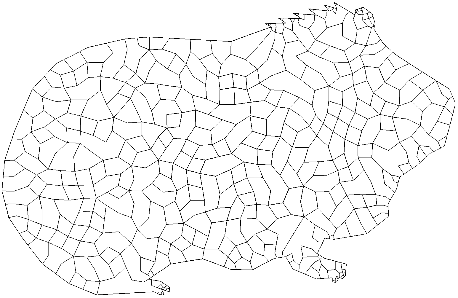
Figure 1: Polygonal mesh of a guinea pig using terminal-edge regions as polygons. The initial triangulation of the PLSG was made using Pygalmesh [37] with the constrain of max edge size of $100$. The resulting input triangulation contains $1330$ triangles, $819$ vertices and $2148$ edges. The output polygonal mesh contains $363$ polygons, $819$ vertices and $1441$ edges.

In this paper we present a GPU parallel algorithm to generate a new kind of 2D polygonal meshes using the concept of terminal-edge regions. This algorithm belongs to the indirect methods. An example of a polygonal mesh generated by the algorithm is shown in Figure 1. The data structure and several kernels to work with the input triangulation and build the arbitrary shape polygons in GPU are described. In particular, the AtomicAdd function is used to manage the concurrent saving of polygons in an array.

This paper is organized as follows: Section LABEL:sec:background introduces the concepts necessary to understand the algorithm. Section 2 describes the data structure uses to represent the input triangulation and the polygonal mesh in the GPU. Section 3 presents the sequential algorithm and the parallel algorithm. Section 4 shows performance experiments of the sequential and parallel algorithms. Finally, Section 5 presents the conclusions and the ongoing work in the parallel algorithm.

2 Data structure

The GPU algorithm receives as input a triangulation. Since GPUs (and their programming models) are designed to work efficiently with arrays, we decided to represent the triangulation with an indexed data structure with neighbor indexation [38]. This representation uses 4 arrays, a Vertex array, a Triangle array, a Neighbor array and a Trivertex array.

• The Vertex array stores each point of the triangulation in pairs, each two elements V[2$\cdot i+0$], V[2$\cdot i+1$] in the array is the coordinate to the i-th point in the triangulation.

• The Triangle array contains indices to the Vertex array, each $3$ elements T[3$\cdot i+0$], T[3$\cdot i+1$], T[3$\cdot i+2$] are indices to the vertices of the i-th triangle in the triangulation.

• The Neighbor array stores indices to the Triangle array, each three indices N[3$\cdot i+0$], N[3$\cdot i+1$], N[3$\cdot i+2$] are the indices to a triangle neighbor to the triangle $i$, the values 0, 1 and 2 represents the edges of $i$.

• The Trivertex array, stores the index of one triangle incident to each vertex $i$ in the Vertex array. This array is optional and is only used to accelerate the Reparation phase in section 3.2.3.

This representation has the advantage that it can be easily allocated in the CUDA’s global device memory, it allows us to assign a unique triangle to each thread and it facilitates the traversal between neighbor triangles in constant time. Also, several programs as QHull [22], Triangle [23] and Detri2 [24] store this representation as output, except for the Trivertex array that can be obtained from the Vertex array and the Triangle array, therefore we can integrate external libraries to generate the initial triangulation.

Polygons are represented as a set of vertices, so to store them, the algorithm uses an array of arbitrary length of indices to the Vertex array.

The output polygonal $\tau^{\prime}=(V,E)$ mesh generated by the algorithm is represented as two arrays in the global memory device. The first one is the Mesh array, this array represents each polygon in $\tau^{\prime}$ as a number that indicates its length and a set of vertices in counter-clock wise that are part of the polygon. The second one is the Position array, that stores the index to the position of the first element of each polygon in the Mesh array.

Other two important data structures are: (i) Seed array: a bit array whose values are true only associated to the indices of the algorithm to generate new polygons, (ii) Max array: given a triangle $i$ in the Neighbor array, Max array stores the index $j$ if the implicit edge stored at $3i+j$ contains the longest-edge of the triangle $i$. Both arrays are stored in the global device memory.

3 Algorithm

3.1 Sequential algorithm

The sequential algorithm is actually submitted to a journal for publication; an early pre-print version can be seen in [39].

3.2 GPU parallel algorithm

The general algorithm is shown in 1. The algorithm takes as input a triangulation $\tau_{L}(V,E)$ and generates as output a polygonal mesh. To do so, the algorithm consists of three main phases: label each edge and triangle of $\tau$, traversal inside terminal-edge regions and repair non-simple polygons generated from the last phase. The first two phases have the advantage that they are extremely data-parallel; it is possible to work with each element in $\tau$ independently, so these phases take advantage of the data parallelism capabilities of the GPU programming model. The Reparation phase needs to split a non-simple polygon into two until all their barrier-edge tips are removed, i.e., transformed in frontier-edge endpoints. Since a non-simple polygon can have more than one barrier-edge, this phase will be repeated until all of them are absorbed by a frontier-edge. The experiments described in 4 show us that there are few non-simple polygons after the Traversal phase. Despite the parallel algorithm we designed for this phase, it seems better to use just the sequential version of this phase.

Algorithm 1 Polygonal Mesh generator

1:Initial Triangulation $\tau=(V,E)$

2:Polygonal Mesh $M$

3:Label triangulation $\tau$ $\triangleright$ Algorithm 2

4:Generate polygons $\triangleright$ Algorithm 3

5:do

6:     Remove barrier-edge tips $\triangleright$ Algorithm 5

7:while $M$ contains Barrier-edge tips

8:return Polygonal Mesh

3.2.1 Label Phase

This phase reads a triangulation $\tau=(V,E)$ as input. The objective is to label frontier-edges in $\tau$ to identify the boundary of each terminal-edge region $R_{i}$ in $\tau$ and to select one triangle of each $R_{i}$ to be used as generator of new polygons in the next phase, the Traversal phase. This phase calls three kernels: LabelMax, LabelSeed and LabelFrontier. Those kernels are shown in Algorithm 2 and they are called consecutively.

Algorithm 2 Label phase’s kernels

Initial Triangulation $\tau=(V,E)$

Labeled triangulation $\tau_{L}=(V,E)$

kernel LabelMax($\tau=(V,E)$)

     for all triangle $t_{i}$ in $\tau$ in parallel  do

         Label the longest-edge of $t_{i}$

     end for

end kernel

kernel LabelSeed($\tau=(V,E)$)

     for all edge $e_{i}\in\tau$ in parallel do

         if $e_{i}$ is border terminal-edge then

              Store adjacent triangle as seed triangle

         end if

         Be $t_{a}$ and $t_{b}$ triangles that share $e_{i}$

         if $e_{i}$ is terminal-edge and $a<b$ then

              Store $t_{a}$ as seed triangle

         end if

     end for

end kernel

kernel LabelFrontier($\tau=(V,E))$

     for all edge $e_{i}\in\tau$ in parallel do

         Be $t_{a}$ and $t_{b}$ triangles that share $e_{i}$

         if $e_{i}$ neither the longest-edge of $t_{a}$ nor $t_{b}$ or $e_{i}$ is border-edge then

              Label $e_{i}$ as frontier-edge

         end if

     end for

end kernel

The first kernel, LabelMax assigns a triangle $t$ of $\tau$ to each thread, then it calculates its longest-edge and stores its index ($0$, $1$ or $2$) in the Max Array.

The second kernel, 9, LabelSeed, assigns an edge $e$ of $\tau$ to each thread. It compares two triangles $t_{a}$ and $t_{b}$ that share $e$ and checks if in both triangles, $e$ is the longest-edge. In that case, $e$ is a terminal-edge and the triangle with lower index is set to True in Seed array, for the generation of a new polygon in the next phase. In case $e$ is both a boundary edge and the longest-edge of the triangle $t$, then $e$ is a boundary terminal-edge and $t$ is stored as seed triangle in the Seed array.

Figure 2: Labeled triangulation generated by the Algorithm 2. Solid lines are frontier-edge, dashed lined are internal-edges and terminal-edges. Red triangles are seed triangles.

The third kernel, 20, LabelFrontier, is similar to LabelSeed, but instead of checking if $e$ is the longest-edge in both adjacent triangles $t_{a}$ and $t_{b}$, this kernel checks if $e$ is not the longest-edge of any of the two triangles. In that case $e$ is labeled as frontier-edge and used in the next phase to delimit a new polygon. In case $e$ is a boundary edge, $e$ is labeled as a frontier-edge, independent of the size of $e$.

After the algorithm calls each kernel consecutively, each terminal-edge region $R_{i}$ is delimited by frontier-edges and a seed triangle per $R_{i}$ was stored as is shown in Figure 2. The data of the triangulation $\tau_{L}=(G,V)$ is in global memory and ready to be used in the Traversal phase.

3.2.2 Traversal phase

In this phase, as many polygons are built as triangle indices are marked true in the Seed array. This phase consists in just one kernel, the TraversalTriangulation kernel, and it is shown in Algorithm 3.

Algorithm 3 Travel Phase

1:Seed array $S$, Triangulation $\tau_{L}(V,E)$

2:Mesh array $M$ , Position array $I$.

3:kernel TraversalTriangulation($\tau=(V,E)$)

4:     for all triangle $t_{i}\in$ $S$ in parallel do

5:         $P_{i}\leftarrow$ PolygonConstruction($t$, $\tau_{L}(V,E)$)

6:         Synchronize threads

7:         $i_{mesh}\leftarrow$ AtomicAdd( $i_{Gmesh}$ , $|P|+1$)

8:         $i_{pos}\leftarrow$ AtomicAdd( $i_{Gpos}$ , $1$)

9:         $I[i_{pos}]\leftarrow i_{mesh}$

10:         $M[i_{mesh}]\leftarrow|P|$

11:         for $j\leftarrow 0$ to $|P|$ do

12:              $M[i_{mesh}+1+j]\leftarrow P[j]$

13:         end for

14:     end for

15:end kernel

The TraversalTriangulation kernel uses the labeled triangulation $\tau_{L}$ of the previous phase to build and and store the polygon information in the Mesh array and the Position array. The kernel assigns to each thread a triangle in the Seed array. If $Seed[i]$ is True, triangle $t_{i}$ is used as starting triangle to build a polygon in PolyConstruction (see Algorithm 4). PolyConstruction travels inside a terminal-edge region $R_{i}$ in counter-clock-wise and stores the frontier-edges of each $t$ inside $R_{i}$ as part of the polygon $P_{i}$. As each vertex of $\tau$ is an endpoint of a frontier-edge, PolyConstruction visits all vertices and edges in $R_{i}$. Note that if $t_{i}$ has 3 frontier-edge, $t_{i}$ is stored as the polygon $P_{i}$. An example of the traversal made by PolyConstruction is shown in Figure 3.

Algorithm 4 Polygon construction

1:Seed triangle $t$, Triangulation $\tau_{L}=(V,E)$

2:Polygon $P$ as a set of vertices.

3:function PolyConstruction($t$, $\tau_{L}=(V,E)$)

4:     $P$ $\leftarrow\emptyset$

5:     $v_{next}$, $v_{init}$ $\leftarrow$ Any vertex of $t$

6:     $t_{next}$, $t_{init}$ $\leftarrow$ t

7:     do

8:         if $t_{next}$ has frontier-edges then

9:              Store frontier-edge in $P$ in ccw

10:              $v_{next}$ $\leftarrow$ Last vertex store in $P$

11:              $t_{next}$ $\leftarrow$ Adjacent triangle by an internal-edge in ccw that share $v_{next}$.

12:         end if

13:     while $t_{next}\not=t_{init}$ or $v_{next}\not=v_{init}$

14:     return P

15:end function

After the polygon $P_{i}$ was generated and stored in a register, the TraversalTriangulation kernel stores $P_{i}$ in the Mesh array. Since several threads attempt to store concurrently their generated polygon in the Mesh array, the kernel manages a global index $i_{Gmesh}$ to get a unique index in Mesh array, each thread has to use to append a new polygon. The global index is obtained using AtomicAdd.

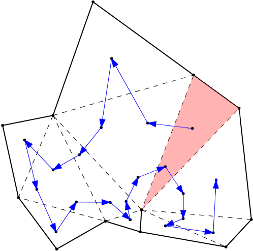
Figure 3: Example of a traversal inside of a terminal-edge region $R_{i}$ to the generation of polygon made by Algoritm 4. Red triangle is the seed triangle of $R_{i}$ and blue arrows are the traversal of the algorithm in $R_{i}$, for each triangle visited with frontier-edges, new edges are added as part of a new polygon.

AtomicAdd returns the value of $i_{Gmesh}$ before the addition, therefore the kernel uses this value as the index position in $i_{Mesh}$ where to store the number of vertices and then the polygon vertices. The $i_{mesh}$ value is stored in the Position array in the same way using the global index $i_{Gpos}$.

After the call to the TraversalTriangulation kernel, the algorithm already has a polygonal mesh $\tau^{\prime}=(V,E)$, stored in the Mesh array and the Position array, but some of their polygons might be non-simple. The next phase, the Reparation phase, is in charge of partitioning non-simple polygons into simple ones.

3.2.3 Reparation phase

In this phase the algorithm repairs non-simple polygons. To do so, the algorithm handles two auxiliary arrays to represent a temporal polygon mesh $\tau^{\prime}_{aux}=(V,E)$: the Aux Mesh array and Aux Position array. The PolygonReparation kernel shown in Algorithm 5 splits each non-simple polygon $P_{i}$ in two new polygons using a diagonal containing a barrier-edge tip of $P_{i}$ and store the result in $\tau^{\prime}_{aux}$. If $\tau^{\prime}_{aux}$ still contains barrier-edge tips, PolygonReparation kernel with $\tau^{\prime}_{aux}$ as input mesh is called again. This process continues until all the barrier-edge tips are removed.

Algorithm 5 Reparation Phase

1:Mesh array $M_{in}$, Position array $I_{in}$, Labeled triangulation $\tau_{L}(V,E)$

2:Mesh array $M_{out}$, Position array $I_{out}$

3:kernel PolygonReparation($\{M_{in},I_{in}\}$, $\tau_{L}$)

4:     for all polygon $P_{i}$ in $\{M_{in},I_{in}\}$ in parallel do

5:         for all consecutive vertices $v_{a}$, $v_{b}$, $v_{c}$ $\in P_{i}$ do

6:              if $v_{a}$ equals $v_{c}$ then

7:                  $v_{bet}\leftarrow v_{b}$

8:                  break

9:              end if

10:         end for

11:         if $v_{bet}\not=\emptyset$ then

12:              $e_{i}\leftarrow$ Middle internal-edge incident to $v_{bet}$

13:              Label $e_{i}$ as frontier-edge

14:              Be $t_{a}$ and $t_{b}$ triangles that share $e_{i}$

15:              $P_{a}$ $\leftarrow$ PolyConstruction($t_{a}$, $\tau_{L}(V,E)$)

16:              $P_{b}$ $\leftarrow$ PolyConstruction($t_{b}$, $\tau_{L}(V,E)$)

17:              Store $P_{a}$ and $P_{b}$ in $M_{out}$

18:         else

19:              Store $P_{i}$ in $M_{out}$

20:         end if

21:     end for

22:     AtomicAdd(Total bet, $|v_{bet}|$)

23:end kernel

To repair each non-simple polygon in $\tau^{\prime}$, the kernel PolygonReparation assigns to each thread a polygon $P_{i}$. Note that there is two ways to store the temporal polygons in this phase, one is using registers and the second one is reading and constructing the polygon directly in the auxilary mesh. Both ways are possible due to the length of the two new polygons is $|P_{a}|+|P_{b}|=|P|+2$ in case of barrier-edge tip.

The kernel first checks if $P_{i}$ contains a barrier-edge tip by comparing 3 consecutive vertices $v_{a}$, $v_{b}$, $v_{c}\in P_{i}$. If $v_{a}=v_{c}$, then $v_{b}$ is a barrier-edge tip, stored in $v_{bet}$, and used to start the process of repairing $P_{i}$. If the kernel does not detect barrier-edge tips then $P$ is stored as part of the polygonal mesh $\tau^{\prime}_{aux}$. .

Starting from a barrier-edge tip $v_{bet}\in P_{i}$, the algorithm searches for an incident triangle to $v_{bet}$ using the Trivertex array. Through this triangle, all internal edges (diagonals) with $v_{bet}$ as endpoint are looked for and the middle internal-edge $e$ is labeled as a new frontier-edge. This strategy divides $P_{i}$ into two new polygons $P_{a}$ and $P_{b}$. The two adjacent triangles $t_{a},t_{b}$ to $e$ are stored and used as seed triangles to generate $P_{a},P_{b}$ by calling Algorithm 4. This process is shown in Figure 4. To store the polygons in $\tau^{\prime}_{aux}$, AtomicAdd is used again with two global indices in the same way as in Algorithm 3.

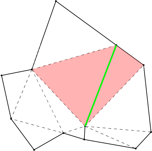
Figure 4: Example of reparation of polygon shown in Figure 3. Green edge is the middle-edge choose to split the polygon. This edge is label as frontier-edge and their two adjacent triangles, in red, are uses to generate two new polygons by calling to Algorithm 4.

At the end of the kernel, AtomicAddis called again with the global variable Total bet, to check if there are further barrier-edge tips. The kernel Total bet PolygonReparation is called again until Total bet gets the value $0$.

The final output is polygonal mesh $\tau^{\prime}=(V,E)$ with simple polygons of arbitrary shape.

4 Experiments

For testing the algorithm, we used a computer with a CPU Intel(R) Core(TM) i5-9600K of 3.70GHz and a GPU NVIDIA GeForce RTX 2060 SUPER. The algorithm was programmed in CUDA C++. The input are random point sets inside a square of sides 10000x10000 stored in point files .node. We used the software Triangle [23] to generate a Delaunay triangulation with the parameters -zn in the triangle file .ele and the neighbor file .neigh. In addition, we created a script to generate the triangle per vertex file .trivertex to accelerate the reparation phase. All polygonal meshes were generated using $65535$ blocks and $1024$ threads per block. An example of the kind of meshes generated in the experiments is shown in Figure 5. We also did a preliminary assess of the resulting polygonal meshes with the virtual element method (VEM) and the result is shown in Figure 6.

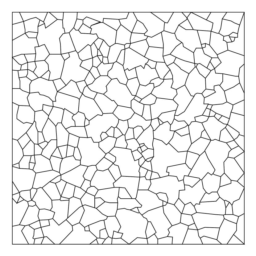
Figure 5: Kind of polygonal mesh generated in the experiments. This mesh was generated using 10000 random poins.

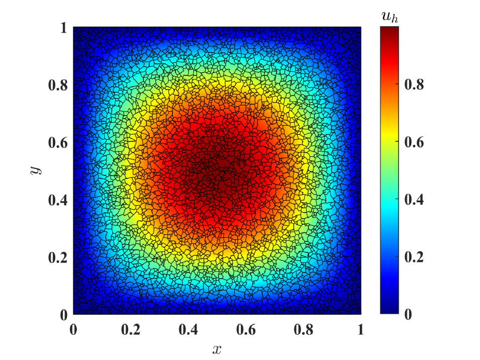
Figure 6: Preliminary simulation results using a polygonal mesh and the Virtual Element Method for a problem modeled with the Laplace equation.

We used the same input trianngulations, varying from 1 million to 8 million points, to compare the time performance of the parallel version, the sequential version and a mixed version. The mixed version uses the parallel version of the label phase and Traversal phase and the sequential version of the Reparation phase. Each test was repeated five times; the average time of the experiments is shown in Figure 8. As we said previously, traversal phase can generate simple and non-simple polygons. The number of non-simple polygons generated in the experiments and needed to be repaired are shown in Figure 7.

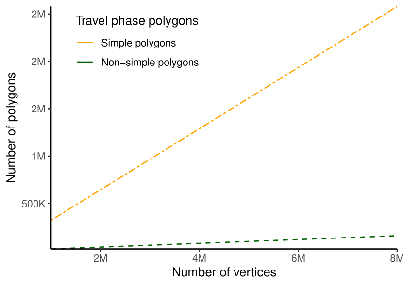
Figure 7: Kind of polygons generated after the travel phase shown in Algorithm 3

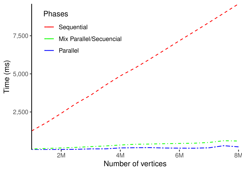
Figure 8: Comparison between the time of the sequential version of the algorithm and the parallel version

The average time of each phase is shown in Figure 9. The faster phase is the traversal phase; this is the simplest kernel since it just calls one kernel once and is applied to a subset of triangles instead to the whole domain. The phase that takes longer was the Label phase. This phase consist in the call to $3$ kernels applied to the edges and triangles of whole triangulation. Figure 10 shows the time of each kernel; the slowest kernel is the Labelmax kernel. This can be explained due to the floating-point arithmetic used to calculate the length of each edge of the input triangulation. The most inefficient parallel phase is the reparation phase, as shown in Figure 7. The number of polygons to repair are very few in contrast with the time that this phase takes. There is no significant advantage of using the parallel version over the sequential version in this phase.

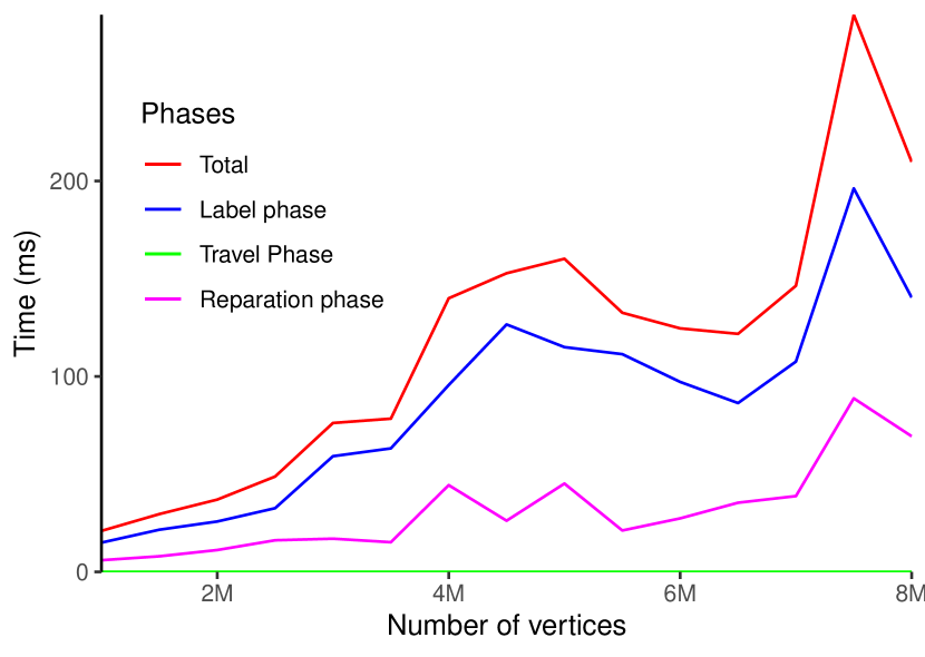
Figure 9: Comparison between the time of each phase in parallel, “Total” refers to the sum of the time of all phases.

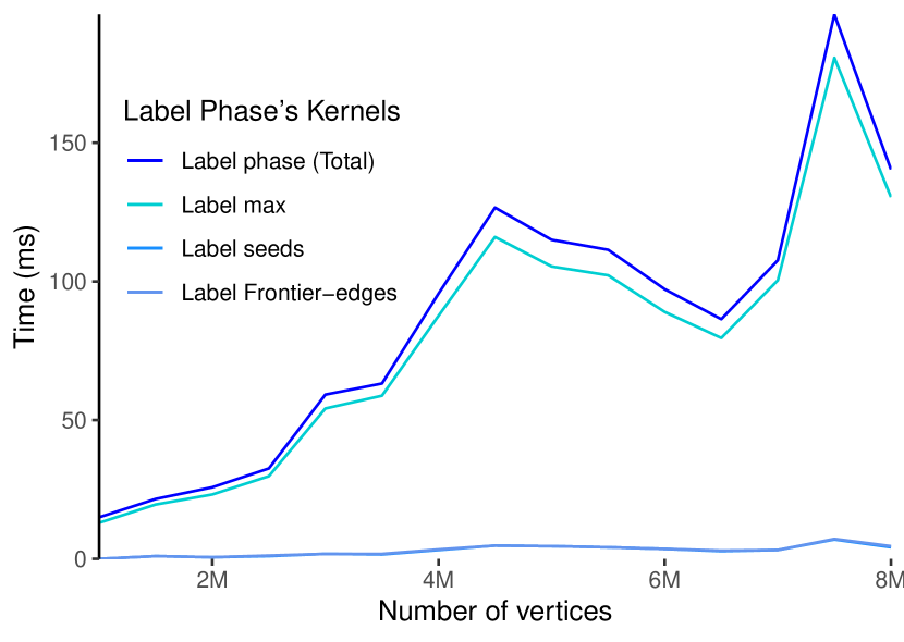
Figure 10: Comparison between the $3$ kernels that are called in the label phase and where shown in Algorithm 2.

5 Conclusions and future work

We have presented an algorithm to build a polygonal mesh formed by convex and non-convex polygons in parallel on GPU-architectures. We hope that this kind of polygonal meshes can be used as an alternative of constrained Voronoi meshes in polygonal finite element methods such as the VEM. Note that Voronoi cells must be cut against the boundary of the input geometry. Terminal-edge regions are always inside the domain.

Our preliminary experimental results show that the GPU programming model allow us to accelerate the sequential version but we still want to do further experiments before computing the speedup. Memory improvements are also necessary in order to minimize the number of read and write operations over the global device memory. The possibility of using shared memory to manage the polygonal mesh should also be evaluated. Using AtomicAdd to manage the index of the polygonal mesh between concurrent threads works with meshes of size inferior to $8$ millions of vertices, but we still have to solve memory problems to generate larger meshes.

We believe that some of the ideas implemented in the Label and Traversal phase can be adapted to accelerate algorithms based on the Longest-edge propagation path on GPU.

References

- [1] Attene M., Campen M., Kobbelt L. “Polygon Mesh Repairing: An Application Perspective.” ACM Comput. Surv., vol. 45, no. 2, Mar. 2013
- [2] Huisman O., de By R. Principles of geographic information systems : an introductory textbook. 01 2009
- [3] Ho-Le K. “Finite element mesh generation methods: a review and classification.” Computer-Aided Design, vol. 20, no. 1, 27–38, 1988
- [4] Ghosh S., Mallett R. “Voronoi cell finite elements.” Computers and Structures, vol. 50, no. 1, 33–46, 1994
- [5] Beir L., Brezzi F., Arabia S. “Basic principles of Virtual Element Methods.” Mathematical Models and Methods in Applied Sciences, vol. 23, 199–214, 2013
- [6] Chi H., da Veiga L.B., Paulino G. “Some basic formulations of the virtual element method (VEM) for finite deformations.” Computer Methods in Applied Mechanics and Engineering, vol. 318, 148–192, 2017
- [7] Park K., Chi H., Paulino G.H. “On nonconvex meshes for elastodynamics using virtual element methods with explicit time integration.” Computer Methods in Applied Mechanics and Engineering, vol. 356, 669–684, 2019
- [8] Attene M., Biasotti S., Bertoluzza S., Cabiddu D., Livesu M., Patanè G., Pennacchio M., Prada D., Spagnuolo M. “Benchmarking the geometrical robustness of a Virtual Element Poisson solver.” Mathematics and Computers in Simulation, vol. 190, 1392–1414, 2021
- [9] Sorgente T., Prada D., Cabiddu D., Biasotti S., Patanè G., Pennacchio M., Bertoluzza S., Manzini G., Spagnuolo M. “VEM and the Mesh.” CoRR, vol. abs/2103.01614, 2021
- [10] Cheng S.W., Dey T.K., Shewchuk J., Sahni S. Delaunay mesh generation. CRC Press Boca Raton, FL, 2013
- [11] Yan D.M., Wang W., Lévy B., Liu Y. “Efficient computation of clipped Voronoi diagram for mesh generation.” Computer-Aided Design, vol. 45, no. 4, 843–852, 2013. Geometric Modeling and Processing 2010
- [12] Yan D.M., Wang K., Levy B., Alonso L. “Computing 2D Periodic Centroidal Voronoi Tessellation.” 2011 Eighth International Symposium on Voronoi Diagrams in Science and Engineering, pp. 177–184. 2011
- [13] Talischi C., Paulino G.H., Pereira A., Menezes I.F. “PolyMesher: a general-purpose mesh generator for polygonal elements written in Matlab.” Structural and Multidisciplinary Optimization, vol. 45, no. 3, 309–328, 2012
- [14] Löhner R. “Progress in grid generation via the advancing front technique.” Engineering with computers, vol. 12, no. 3-4, 186–210, 1996
- [15] Bommes D., Lévy B., Pietroni N., Puppo E., Silva C., Tarini M., Zorin D. “Quad-mesh generation and processing: A survey.” Computer Graphics Forum, vol. 32, pp. 51–76. Wiley Online Library, 2013
- [16] Owen S.J., Staten M.L., Canann S.A., Saigal S. “Q-Morph: an indirect approach to advancing front quad meshing.” International journal for numerical methods in engineering, vol. 44, no. 9, 1317–1340, 1999
- [17] Owen S.J. “A survey of unstructured mesh generation technology.” IMR, vol. 239, 267, 1998
- [18] Johnen A. Indirect quadrangular mesh generation and validation of curved finite elements. Ph.D. thesis, Université de Liège, Liège, Belgique, 2016
- [19] Lee C., Lo S. “A new scheme for the generation of a graded quadrilateral mesh.” Computers & Structures, vol. 52, no. 5, 847–857, 1994
- [20] Remacle J.F., Lambrechts J., Seny B., Marchandise E., Johnen A., Geuzainet C. “Blossom-Quad: A non-uniform quadrilateral mesh generator using a minimum-cost perfect-matching algorithm.” International Journal for Numerical Methods in Engineering, vol. 89, no. 9, 1102–1119, 2012
- [21] Merhof D., Grosso R., Tremel U., Greiner G. “Anisotropic quadrilateral mesh generation : an indirect approach.” Advances in Engineering Software, vol. 38, no. 11/12, 860–867, 2007
- [22] Barber C.B., Dobkin D.P., Huhdanpaa H. “The Quickhull Algorithm for Convex Hulls.” ACM Trans. Math. Softw., vol. 22, no. 4, 469–483, Dec. 1996
- [23] Shewchuk J.R. “Triangle: Engineering a 2D quality mesh generator and Delaunay triangulator.” M.C. Lin, D. Manocha, editors, Applied Computational Geometry Towards Geometric Engineering, pp. 203–222. Springer Berlin Heidelberg, Berlin, Heidelberg, 1996
- [24] Si H. “An Introduction to Unstructured Mesh Generation Methods and Softwares for Scientific Computing.” Course, 7 2019. 2019 International Summer School in Beihang University
- [25] Chrisochoides N. “Parallel Mesh Generation.” A.M. Bruaset, A. Tveito, editors, Numerical Solution of Partial Differential Equations on Parallel Computers, pp. 237–264. Springer Berlin Heidelberg, Berlin, Heidelberg, 2006
- [26] Löhner R. “A 2nd Generation Parallel Advancing Front Grid Generator.” X. Jiao, J.C. Weill, editors, Proceedings of the 21st International Meshing Roundtable, pp. 457–474. Springer Berlin Heidelberg, Berlin, Heidelberg, 2013
- [27] Chernikov A.N., Chrisochoides N.P. “Algorithm 872: Parallel 2D Constrained Delaunay Mesh Generation.” ACM Trans. Math. Softw., vol. 34, no. 1, Jan. 2008
- [28] Bern M., Eppstein D., Teng S.h. “Parallel Construction Of Quadtrees And Quality Triangulations.” International Journal of Computational Geometry & Applications, vol. 09, no. 06, 517–532, 1999
- [29] Barragán A., Reeve J. “A Two-Dimensional parallel quadtree finite element mesh generator.” Parallel Computing: Fundamentals and Applications, pp. 251–258. World Scientific, 2000
- [30] Hoff K.E., Keyser J., Lin M., Manocha D., Culver T. “Fast Computation of Generalized Voronoi Diagrams Using Graphics Hardware.” Proceedings of the 26th Annual Conference on Computer Graphics and Interactive Techniques, SIGGRAPH ’99, p. 277–286. ACM Press/Addison-Wesley Publishing Co., USA, 1999
- [31] Fischer I., Gotsman C. “Fast Approximation of High-Order Voronoi Diagrams and Distance Transforms on the GPU.” Journal of Graphics Tools, vol. 11, no. 4, 39–60, 2006
- [32] Cao T.T., Tang K., Mohamed A., Tan T.S. “Parallel Banding Algorithm to Compute Exact Distance Transform with the GPU.” Proceedings of the 2010 ACM SIGGRAPH Symposium on Interactive 3D Graphics and Games, I3D ’10, p. 83–90. Association for Computing Machinery, New York, NY, USA, 2010
- [33] Rong G., Tan T.S., Cao T.T., Stephanus. “Computing Two-Dimensional Delaunay Triangulation Using Graphics Hardware.” Proceedings of the 2008 Symposium on Interactive 3D Graphics and Games, I3D ’08, p. 89–97. Association for Computing Machinery, New York, NY, USA, 2008
- [34] Qi M., Cao T.T., Tan T.S. “Computing 2D Constrained Delaunay Triangulation Using the GPU.” IEEE Transactions on Visualization and Computer Graphics, vol. 19, no. 5, 736–748, 2013
- [35] Kelly M., Breslow A., Kelly A. “Quad-tree construction on the gpu: A hybrid cpu-gpu approach.” Retrieved June13, 2011
- [36] Navarro C.A., Hitschfeld-Kahler N., Scheihing E. “A GPU-based Method for Generating quasi-Delaunay Triangulations based on Edge-flips.” GRAPP/IVAPP, pp. 27–34. 2013
- [37] Schlömer N. “pygalmesh: Python interface for CGAL’s meshing tools.”
- [38] De Floriani L., Kobbelt L., Puppo E. “A Survey on Data Structures for Level-of-Detail Models.” N.A. Dodgson, M.S. Floater, M.A. Sabin, editors, Advances in Multiresolution for Geometric Modelling, pp. 49–74. Springer Berlin Heidelberg, Berlin, Heidelberg, 2005
- [39] Salinas S., Hitschfeld-Kahler N., Si H. “TR/DCC-2021-2: Studying the properties of polygon meshes built from Delaunay triangulations.” May 2021