Computing a Sparse Projection into a Box

Abstract

We describe a procedure to compute a projection of $w\in\mathds{R}^{n}$ into the intersection of the so-called zero-norm ball $k\mathds{B}_{0}$ of radius $k$, i.e., the set of $k$-sparse vectors, with a box centered at a point of $k\mathds{B}_{0}$. The need for such projection arises in the context of certain trust-region methods for nonsmooth regularized optimization. Although the set into which we wish to project is nonconvex, we show that a solution may be found in $O(n\log(n))$ operations. We describe our Julia implementation and illustrate our procedure in the context of two trust-region methods for nonsmooth regularized optimization.

1 Introduction

We describe a procedure to compute a projection of a point in $\mathds{R}^{n}$ into the intersection of the set of $k$-sparse vectors with a box centered at a $k$-sparse vector.

Specifically, let $\Delta\mathds{B}_{\infty}$ be the $\ell_{\infty}$-norm ball of radius $\Delta\geq 0$ and centered at the origin, and $x+\Delta\mathds{B}_{\infty}$ be the same ball centered at $x\in\mathds{R}^{n}$. The set of $k$-sparse vectors in $\mathds{R}^{n}$, otherwise known as the $\ell_{0}$-pseudonorm ‘‘ball’’ of radius $k\in\{0,1,\ldots,n\}$, is denoted $k\mathds{B}_{0}$ and is the set of vectors with at most $k$ nonzero components. Assume that $x\in k\mathds{B}_{0}$. For given $w\in\mathds{R}^{n}$, we seek to compute

$$p(w)\in P(w):=\mathop{\textup{argmin}}\ \{\|w-y\|_{2}\mid y\in C\}\qquad C:=k\mathds{B}_{0}\cap(x+\Delta\mathds{B}_{\infty}).$$ (1)

Because $C$ is closed, $P(w)\neq\varnothing$, but because $C$ is nonconvex, $P(w)$ may contain several elements. In (1), we seek a global minimum---local nonglobal minima sometimes exist, but are of no particular interest here. Although it may appear as though the problem has exponential complexity due to the combinatorial nature of $k$-sparsity, we show that a solution may be found in $O(n\log(n))$ operations. We describe our Julia implementation and illustrate our procedure in the context of two trust-region methods for nonsmooth regularized optimization.

Context

The computation of (1) occurs in the evaluation of proximal operators encountered during the iterations of the trust-region method of Aravkin et al. [1] for nonsmooth regularized optimization. Their method is designed for problems of the form

$$\mathop{\textup{minimize}}_{x\in\mathds{R}^{n}}\ f(x)+h(x),$$ (2)

where $f:\mathds{R}^{n}\to\mathds{R}$ has Lipschitz-continuous gradient and $h:\mathds{R}^{n}\to\mathds{R}\cup\{\pm\infty\}$ is lower semi-continuous and proper. In large-scale data fitting and signal reconstruction problems, $h(x)=\chi(x\mid k\mathds{B}_{0})$ encodes sparsity constraints and is of interest if one is to recover a solution with at most $k$ nonzero elements, where $\chi(\cdot\mid A)$ is the indicator of $A\subseteq\mathds{R}^{n}$, i.e.,

$$\chi(x\mid A)=\begin{cases}0&\text{if }x\in A,\\ \infty&\text{otherwise}.\end{cases}$$

All iterates $x_{j}$ generated are feasible in the sense that $x_{j}\in k\mathds{B}_{0}$. At iteration $j$, a step $s$ is computed in

$$\mathop{\textup{argmin}}_{u}\tfrac{1}{2}\|u-v\|_{2}^{2}+h(x_{j}+u)+\chi(u\mid\Delta_{j}\mathds{B}_{\infty}),$$

where $v\in\mathds{R}^{n}$ is given and $\Delta_{j}\mathds{B}_{\infty}$ is the trust region centered at the origin of radius $\Delta_{j}>0$. With the change of variables $z:=x_{j}+u$, we may rewrite the above as

$$\mathop{\textup{argmin}}_{z}\ \tfrac{1}{2}\|z-w\|_{2}^{2}+\chi(z\mid k\mathds{B}_{0})+\chi(z\mid x_{j}+\Delta_{j}B_{\infty})-\{x_{j}\},$$

where $w:=x_{j}+v$, which precisely amounts to (1) with $x_{j}$ in the role of $x$ and $\Delta_{j}$ in the role of $\Delta$ because the two indicators may be combined into the indicator of the intersection.

Because nonsmooth regularized problems often involve a nonlinear least squares smooth term, Aravkin et al. [2] develop a Levenberg-Marquardt variant of their trust region method. The latter requires the same projections as just described.

Notation

Let $\mathop{\textup{supp}}(x):=\{i=1,\ldots,n\mid x_{i}\neq 0\}$ be the support of $x$. If $A\subseteq\mathds{R}^{n}$ is closed and $A\neq\varnothing$, we denote

$$\mathop{\textup{proj}}(w\mid A):=\mathop{\textup{argmin}}\ \{\|w-y\|_{2}\mid y\in A\},$$

the projection of $w$ into $A$, which is a set with at least one element.

When the projection of $w$ into $A$ is unique, such as happens when $A$ is convex, we slightly abuse notation and write $y=\mathop{\textup{proj}}(w\mid A)$ instead of $\{y\}=\mathop{\textup{proj}}(w\mid A)$.

If $B\subseteq\mathds{R}^{n}$, the notation $\mathop{\textup{proj}}(\mathop{\textup{proj}}(w\mid A)\mid B)$ refers to the set $\{z\in\mathop{\textup{proj}}(y\mid B)\text{ for some }y\in\mathop{\textup{proj}}(w\mid A)\}$.

If $S\subseteq\{1,\ldots,n\}$, the cardinality of $S$ is denoted $|S|$, and its complement is $S^{c}$. For such $S$ and for $x\in\mathds{R}^{n}$, we denote $x_{S}$ the subvector of $x$ indexed by $S$ and $A_{S}:=\{x\in\mathds{R}^{n}\mid x_{S^{c}}=0\}$. Clearly, $0\in A_{S}$ for any such $S$.

Because

$$k\mathds{B}_{0}=\bigcup\ \{A_{S}\mid S\subseteq\{1,\ldots,n\},\ |S|=k\},$$

[5, p. $175$], we refer to $A_{S}$ as a piece of $k\mathds{B}_{0}$.

Related Research

Duchi et al. [11] describe how to project efficiently into the $\ell_{1}$-norm ball. The $\ell_{1}$-norm is probably the most widely used convex approximation of the $\ell_{0}$ norm as minimizing $\|x\|_{1}$ promotes sparsity under certain conditions---see, e.g., [10] and the vast ensuing compressed sensing literature.

Gupta et al. [12] describe how to project into the intersection of an $\ell_{1}$-norm ball with a box, which may be seen as a relaxation of (1). Thom and Palm [17] and Thom et al. [18] propose a linear-time and constant space algorithm to compute a projection into a hypersphere with a prescribed sparsity, where sparsity is measured by the ratio of the $\ell_{1}$ to the $\ell_{2}$ norm.

Beck and Eldar [6] provide optimality conditions for the minimization of a smooth function over $k\mathds{B}_{0}$. Beck and Hallak [7] provide optimality conditions for problems of the form (1) where the box is replaced with a symmetric set satisfying certain conditions. Unfortunately, (1) does not satisfy those conditions unless $x=0$, at which point it is easy to see that a solution simply consists in chaining the projection into $k\mathds{B}_{0}$ with that into $\Delta\mathds{B}_{\infty}$. That is what Luss and Teboulle [15, Proposition $4.3$] do with $1\mathds{B}_{2}$ instead of $\Delta\mathds{B}_{\infty}$.

Bolte et al. [9, Proposition $4$] show how to project into the intersection of $k\mathds{B}_{0}$ with the nonnegative orthant.

Kyrillidis et al. [13] explain how to compute a sparse projection into the simplex, which is probably the most closely related research to our objectives. The simplex necessarily intersects all pieces of $k\mathds{B}_{0}$, which need not be the case for (1).

2 Geometric Intuition

Naively chaining the projection into one set with that into the other, in either order, does not necessarily yield a point into the intersection of the two sets, even if the latter are convex. Figures 1 and 2 illustrates two situations that we may encounter when $k=1$ and $n=2$.

A few simple observations about Figures 1 and 2 reveal some difficulties associated with the computation of $p(w)$:

1. because both components of $w_{1}$ are equal in absolute value, as indicated by the thin diagonal in Figure 2, $\mathop{\textup{proj}}(w_{1}\mid k\mathds{B}_{0})$ is a set with two elements, and projecting those into $x+\Delta\mathds{B}_{\infty}$ yields $p(w_{1})$ (the correct global minimum) and $p_{2}$ (a spurious local minimum);

2. moving $w_{1}$ up slightly would preserve $p(w_{1})$, but projecting into $1\mathds{B}_{0}$ first would lead to $p_{2}$;

3. moving $w_{1}$ slightly to the right would result in a projection that is slightly to the right of $p(w_{1})$ on the figure, but projecting into $1\mathds{B}_{0}$ first would lead to $p_{2}$;

4. moving $w_{1}$ further to the right would result in $P(w_{1})=\{p(w_{1}),p_{2}\}$ and moving it further still would result in $P(w_{1})=\{p_{2}\}$;

5. in the rightmost plot, chaining the projections either way leads to a point that does not even lie in the intersection.

  

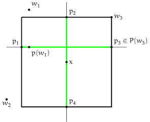
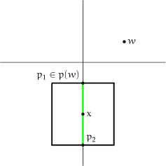
Figure 1: The set composed of the two axes is $1\mathds{B}_{0}$ in $\mathds{R}^{2}$, the box is $x+\Delta\mathds{B}_{\infty}$ and the green set is their intersection. Left: $P(w_{1})=\{p(w_{1})\}$, and $P(w_{2})=\{p_{1}\}$. With respect to $w_{1}$, the other cardinal points are $p_{2}$, a local minimum, $p_{3}$, a local maximum, and $p_{4}$, a global maximum. Right: the intersection of $1\mathds{B}_{0}$ with $x+\Delta\mathds{B}_{\infty}$ is entirely determined by $\mathop{\textup{supp}}(x)$, $P(w)=\{p_{1}\}$ while $p_{2}$ is a global maximum.

  

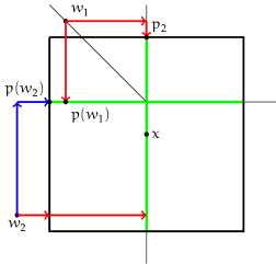
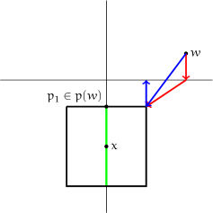
Figure 2: Simply composing the projection into $1\mathds{B}_{0}$ with that into $x+\Delta\mathds{B}_{\infty}$, in either order, may lead to an erroneous projection.

Note that $1\mathds{B}_{0}$ is a special case for any value of $n$: its intersection with $x+\Delta\mathds{B}_{\infty}$ consists in either a single line segment, or $n$ segments. Indeed, the first possibility is that the nonzero component of $x$ is $|x_{i}|>\Delta$. In that case, any $y\in 1\mathds{B}_{0}$ with $y_{j}\neq 0$ and $i\neq j$ satisfies $\|y-x\|_{\infty}\geq|x_{i}|>\Delta$, and therefore $y\not\in x+\Delta\mathds{B}_{\infty}$. The only other possibility is that $|x_{i}|\leq\Delta$, in which case $0\in x+\Delta\mathds{B}_{\infty}$, and therefore, all pieces of $1\mathds{B}_{0}$ intersect the box.

For $1<k<n$, however, the intersection may consist in any number of pieces between $1$ and ${n\choose k}$.

Figure 3 illustrates situations that may arise for $k=1$ or $2$ and $n=3$.

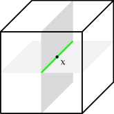
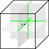
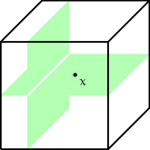
Figure 3: Left: the green segment represents a possible intersection of $1\mathds{B}_{0}$ with a box in $\mathds{R}^{3}$. The gray plane sections only serve to position the segment visually in three dimensions. Center: another possible intersection of $1\mathds{B}_{0}$ with a box in $\mathds{R}^{3}$. The box either intersects a single axis, or all of them. Right: the green region is a possible intersection of $2\mathds{B}_{0}$ with a box in $\mathds{R}^{3}$. The gray segment only serves as a visual aid and is part of the intersection.

3 Background and Preliminary Results

The unique projection $y$ of any $w$ into $x+\Delta\mathds{B}_{\infty}$ has components

$$y_{i}=\max(x_{i}-\Delta,\min(w_{i},x_{i}+\Delta)),\quad i=1,\ldots,n.$$

Given $S\subseteq\{1,\ldots,n\}$, we obtain the unique projection of any $w$ into $A_{S}$ by setting $w_{i}=0$ for all $i\in S^{c}$.

A projection $y$ of any $w$ into $k\mathds{B}_{0}$ is a vector that has the same $k$ largest components in absolute value as $w$, and the rest of its components set to zero [5, Lemma $6.71$].

In the vein of Beck and Eldar [6], it is possible to state necessary optimality conditions for the more general problem

$$\mathop{\textup{minimize}}_{y\in\mathds{R}^{n}}\ f(y)\quad\textup{subject to}\ y\in C,$$ (3)

of which (1) is a special case. Despite the fact that our algorithm is not based on such necessary conditions, they are relevant in their own right, and we now review and specialize them to (1).

Lemma 1.

Let $y^{\star}$ be a solution of (3) where $f$ is continuously differentiable.

1. If $\|y^{\star}\|_{0}<k$, then for all $i=1,\ldots,n$,

   $$\frac{\partial f(y^{\star})}{\partial y_{i}}\begin{cases}\leq 0&\text{ if }y^{\star}_{i}=x_{i}+\Delta\\ \geq 0&\text{ if }y^{\star}_{i}=x_{i}-\Delta\\ =0&\text{ otherwise;}\end{cases}$$

2. if $\|y^{\star}\|_{0}=k$, the same conditions hold for all $i\in\mathop{\textup{supp}}(y^{\star})$.

Proof.

The proof follows that of [6, Theorem $2.1$]. If $\|y^{\star}\|_{0}<k$, then for all $i=1,\ldots,n$,

$$0\in\mathop{\textup{argmin}}_{t\in\mathds{R}}\ \{g(t)\mid\|y^{\star}+te_{i}-x\|_{\infty}\leq\Delta\},$$

where $e_{i}$ is the $i$-th column of the identity, and $g(t):=f(y^{\star}+te_{i})$.

Because $y^{\star}\in x+\Delta\mathds{B}_{\infty}$, the constraint above reduces to $|y^{\star}_{i}+t-x_{i}|\leq\Delta$. The conclusion follows directly from the standard KKT conditions by noting that $g^{\prime}(0)=\partial f(y^{\star})/\partial y_{i}$.

If $\|y^{\star}\|_{0}=k$, the same reasoning goes for all $i\in\mathop{\textup{supp}}(y^{\star})$. ∎

By analogy with [6, Theorem $2.1$], a candidate satisfying the conditions of Lemma 1 is called a basic feasible point. The following corollary follows directly from Lemma 1 with $f(y):=\tfrac{1}{2}\|w-y\|_{2}^{2}$.

Corollary 1.

Let $y^{\star}$ be a solution of (1).

1. If $\|y^{\star}\|_{0}<k$, then for all $i=1,\ldots,n$,

   $$y^{\star}_{i}\begin{cases}\leq w_{i}&\text{ if }y^{\star}_{i}=x_{i}+\Delta\\ \geq w_{i}&\text{ if }y^{\star}_{i}=x_{i}-\Delta\\ =w_{i}&\text{ otherwise;}\end{cases}$$

2. if $\|y^{\star}\|_{0}=k$, the same conditions hold for all $i\in\mathop{\textup{supp}}(y^{\star})$.

Lemma 1 and Corollary 1 are only necessary conditions, and they are rather weak; there often exist vectors satisfying the conditions stated that are not solutions of (3) or (1). Consider for example $k=1$ in $\mathds{R}^{2}$, $x=(0,-1)$, $\Delta=2$, and $w=(2,3)$. Then, $y=(2,0)$ satisfies the conditions of Corollary 1: $\|y\|_{0}=1$, $\mathop{\textup{supp}}(y)=\{1\}$ and $y_{1}=x_{1}+\Delta\leq w_{1}$. However, $P(w)=\{(0,1)\}$. Indeed, $\|w-(0,1)\|=2\sqrt{2}<3=\|w-y\|$.

Observe that thanks to [6, Lemma $2.1$], the number of basic feasible points of (1) is finite. Therefore, so is the cardinality of $P(w)$.

For a constant $L>0$, Beck and Eldar define $y\in C$ to be $L$-stationary for (3) if it satisfies $y\in\mathop{\textup{proj}}(y-L^{-1}\nabla f(y)\mid C)$, a condition insipired by optimality conditions for convex problems. They state the following result, whose proof remains valid for (3).

Lemma 2 (6, Lemma $2.2$).

For any $L>0$, $y\in\mathds{R}^{n}$ is $L$-stationary for (3) if and only if $y\in C$ and

$$\frac{\partial f(y)}{\partial y_{i}}=0\quad(i\in\mathop{\textup{supp}}(y))\qquad\text{and}\qquad\left|\frac{\partial f(y)}{\partial y_{i}}\right|\leq LM_{k}(y)\quad(i\not\in\mathop{\textup{supp}}(y)),$$

where $M_{k}(y)$ is the $k$th largest component of $y$ in absolute value.

With $f(y):=\tfrac{1}{2}\|w-y\|_{2}^{2}$, $L$-stationarity reads $y\in\mathop{\textup{proj}}(y-L^{-1}(y-w)\mid C)$. Due to the simple form of $\nabla f(y)=y-w$, Lemma 2 specializes as follows.

Corollary 2.

For any $L>0$, $y\in\mathds{R}^{n}$ is $L$-stationary for (1) if and only if $y\in C$ and

$$w_{i}=y_{i}\quad(i\in\mathop{\textup{supp}}(y)),\qquad\text{and}\qquad|w_{i}|\leq LM_{k}(y)\quad(i\not\in\mathop{\textup{supp}}(y)).$$

As a special case of Corollary 2, if $\|y\|_{0}<k$, then $M_{k}(y)=0$ and we obtain $w_{i}=0$ for $i\not\in\mathop{\textup{supp}}(y)$. In that case, $L$-stationarity turns out to be independent of $L$ and requires that $y=w$, i.e., there is a unique $L$-stationary point if $w\in C$, and there are no $L$-stationary points if $w\not\in C$.

$L$-stationarity is stronger than basic feasibility in the sense that if $y$ is $L$-stationary for (3) for any $L>0$, then $y$ is also a basic feasible point [6, Corollary$2.1$].

Under a Lipschitz assumption, solutions of (3) are $L$-stationary, as stated in the following result.

Proposition 1 (6, Theorem $2.2$).

Assume $\nabla f$ is Lipschitz continuous with constant $L_{f}$ and $y$ solves (3). Then, for any $L>L_{f}$,

1. $y$ is $L$-stationary;

2. $\mathop{\textup{proj}}(y-L^{-1}\nabla f(y)\mid C)$ is a singleton.

Proof.

The proof follows by verifying that [6, Lemma $2.4$] continues to hold for (3) and the proof of [6, Theorem $2.2$] holds unchanged. ∎

Proposition 1 clearly applies to (1) as the gradient of $f(y):=\tfrac{1}{2}\|w-y\|_{2}^{2}$ is Lipschitz continuous with constant $L_{f}=1$. Thus, solutions of (1) are $L$-stationary for $L>1$.

Based on $L$-stationarity, Beck and Eldar [6] study the iteration $y^{+}\in\mathop{\textup{proj}}(y-L^{-1}\nabla f(y)\mid C)$ and show convergence to an $L$-stationary point for (3) under the assumption that $\nabla f$ is Lipschitz continuous. Unfortunately, in the case of (1), solving the subproblem is as difficult as solving (1) directly.

Finally, Beck and Eldar define the concept of componentwise (CW) optimality as follows: $y\in C$ is CW-minimum for (3) if

1. $\|y\|_{0}<k$ and $f(y)=\min_{t}f(y+te_{i})$ for $i=1,\dots,n$, or

2. $\|y\|_{0}=k$ and $f(y)\leq\min_{t}f(y-y_{i}e_{i}+te_{j})$ for $i\in\mathop{\textup{supp}}(y)$ and $j=1,\dots,n$.

They observe that any solution is a CW-minimum [6, Theorem $2.3$] and that any CW-minimum is a basic feasible point [6, Lemma $2.5$]. The concept of CW-minimum allows them to show that any solution of (3) is $L$-stationary for a value $L$ that can be significantly smaller than $L_{f}$. Based on those observations, they propose two coordinate descent-type methods that converge to a CW-minimum.

In the next section, we present a number of properties of (1) and an algorithm that identifies a solution directly, without resort to the above stationarity conditions.

4 Computing the Projection

We begin with a few simple observations.

Lemma 3.

Let $S\subseteq\{1,\ldots,n\}$ such that $|S|=k$. If $y\in x+\Delta\mathds{B}_{\infty}$ and $z=\mathop{\textup{proj}}(y\mid A_{S})$, then $\|z-x\|_{\infty}\leq\|y-x\|_{\infty}$ and, in particular, $z\in x+\Delta\mathds{B}_{\infty}$.

Proof.

Without loss of generality, we may write $z=(y_{S},0)$. Observe now that

$$\Delta\geq\|y-x\|_{\infty}=\max(\|y_{S}-x_{S}\|_{\infty},\|y_{S^{c}}-x_{S^{c}}\|_{\infty})=\max(\|y_{S}-x_{S}\|_{\infty},\|y_{S^{c}}\|_{\infty})\geq\|y_{S}-x_{S}\|_{\infty}=\|z-x\|_{\infty},$$

because $x_{S^{c}}=0$. ∎

Lemma 3 holds because of the geometry of $k\mathds{B}_{0}$ respective to $\mathds{B}_{\infty}$ and is specific to the $\ell_{\infty}$-norm. Indeed, consider for example a ball defined in the $\ell_{2}$-norm and set $x=(0,-1)\in 1\mathds{B}_{0}$ and $\Delta=2$. For $y_{1}=(\tfrac{3}{4},-\tfrac{1}{4})$, we have $z_{1}=\mathop{\textup{proj}}(y_{1}\mid 1\mathds{B}_{0})=(\tfrac{3}{4},0)$ and $\|z_{1}-x\|_{2}>\|y-x\|_{2}$. In this example, $z_{1}\in x+\Delta\mathds{B}_{2}$, but consider now $y_{2}=(2,-1)$. Then, $z_{2}=\mathop{\textup{proj}}(y_{2}\mid 1\mathds{B}_{0})=(2,0)\not\in x+\Delta\mathds{B}_{2}$.

Lemma 4.

If $w\in x+\Delta\mathds{B}_{\infty}$, then $P(w)=\mathop{\textup{proj}}(w\mid k\mathds{B}_{0})$.

Proof.

Any $y\in\mathop{\textup{proj}}(w\mid k\mathds{B}_{0})$ has the same $k$ largest components in absolute value as $w$, and the rest of its components set to zero. Thus, there must exist $S\subseteq\{1,\ldots,n\}$ with $|S|=k$ such that $y=\mathop{\textup{proj}}(w\mid A_{S})$. By Lemma 3, $\|y-x\|_{\infty}\leq\|w-x\|_{\infty}\leq\Delta$ so that $y\in x+\Delta\mathds{B}_{\infty}$, and hence, $y\in C$. If there were $z\in C$ such that $\|z-w\|_{2}<\|y-w\|_{2}$, because $z\in k\mathds{B}_{0}$, there would be a contradiction with the definition of $y$. Therefore, $y$ is a closest point to $w$ in $C$. ∎

Lemma 5.

$C=A_{\mathop{\textup{supp}}(x)}\cap(x+\Delta\mathds{B}_{\infty})$ if and only if  $|x_{i}|>\Delta$ for all $i\in\mathop{\textup{supp}}(x)$.

Proof.

The result follows from the observation that for any $i\in\mathop{\textup{supp}}(x)$, there is no $y\in x+\Delta\mathds{B}_{\infty}$ with $y_{i}=0$. Indeed, if $y_{i}=0$, $\|y-x\|_{\infty}\geq|y_{i}-x_{i}|=|x_{i}|>\Delta$. ∎

Lemma 6.

For any $S\subseteq\{1,\ldots,n\}$ and any $w\in\mathds{R}^{n}$,

$$\mathop{\textup{proj}}(w\mid A_{S}\cap(x+\Delta\mathds{B}_{\infty}))=\mathop{\textup{proj}}(proj(w\mid x+\Delta\mathds{B}_{\infty})\mid A_{S})=\mathop{\textup{proj}}(proj(w\mid A_{S})\mid x+\Delta\mathds{B}_{\infty}),$$

whose unique element is the vector $y$ such that $y_{S}=\mathop{\textup{proj}}(w_{S}\mid x_{S}+\Delta\mathds{B}_{\infty})$ and $y_{S^{c}}=0$.

In particular, if $C=A_{\mathop{\textup{supp}}(x)}\cap(x+\Delta\mathds{B}_{\infty})$, then $P(w)=\{\mathop{\textup{proj}}(\mathop{\textup{proj}}(w\mid x+\Delta\mathds{B}_{\infty})\mid A_{\mathop{\textup{supp}}(x)})\}$.

Proof.

The projection is unique because $A_{S}\cap(x+\Delta\mathds{B}_{\infty})$ is convex. If $y:=\mathop{\textup{proj}}(w\mid x+\Delta\mathds{B}_{\infty})$ observe that $z:=\mathop{\textup{proj}}(y\mid A_{S})\in A_{S}\cap(x+\Delta\mathds{B}_{\infty})$ by Lemma 3.

In order to show that $z\in\mathop{\textup{proj}}(w\mid A_{S}\cap(x+\Delta\mathds{B}_{\infty}))$, pick any other $\bar{z}\in A_{S}\cap(x+\Delta\mathds{B}_{\infty})$. By construction, $\bar{z}=(\bar{y}_{S},0)$ for some $\bar{y}$. Among the infinitely many possible $\bar{y}$, we may choose the one such that $\bar{y}_{S^{c}}=y_{S^{c}}$. Then,

$$\|w-y\|_{2}^{2}=\|w_{S}-y_{S}\|_{2}^{2}+\|w_{S^{c}}-y_{S^{c}}\|_{2}^{2}=\|w_{S}-z_{S}\|_{2}^{2}+\|w_{S^{c}}-y_{S^{c}}\|_{2}^{2},$$

and

$$\|w-\bar{y}\|_{2}^{2}=\|w_{S}-\bar{y}_{S}\|_{2}^{2}+\|w_{S^{c}}-\bar{y}_{S^{c}}\|_{2}^{2}=\|w_{S}-\bar{z}_{S}\|_{2}^{2}+\|w_{S^{c}}-y_{S^{c}}\|_{2}^{2}.$$

By definition of $y$, $\|w-y\|_{2}\leq\|w-\bar{y}\|_{2}$ and the above therefore implies $\|w_{S}-z_{S}\|_{2}^{2}\leq\|w_{S}-\bar{z}_{S}\|_{2}^{2}$. Because $z_{S^{c}}=\bar{z}_{S^{c}}=0$, we may add $\|w_{S^{c}}\|_{2}^{2}$ to both sides of the previous inequality to obtain $\|w-z\|_{2}\leq\|w-\bar{z}\|_{2}$. ∎

Lemma 5 provides an easily computable criterion to determine that $C=A_{\mathop{\textup{supp}}(x)}\cap(x+\Delta\mathds{B}_{\infty})$, and, thanks to Lemma 6, we find an element of $P(w)$ by setting all components of $\mathop{\textup{proj}}(w\mid x+\Delta\mathds{B}_{\infty})$ that are not in $\mathop{\textup{supp}}(x)$ to zero. Such situation is represented in the rightmost plot of Figure 1.

By Lemma 5, if there is $|x_{i}|\leq\Delta$, then $x+\Delta\mathds{B}_{\infty}$ intersects other pieces of $k\mathds{B}_{0}$ than $A_{\mathop{\textup{supp}}(x)}$. We now determine which pieces, and their number. Let

$$s(x):=\{i\in\mathop{\textup{supp}}(x)\mid|x_{i}|\leq\Delta\}\quad\text{and}\quad\ell(x):=\{i\in\mathop{\textup{supp}}(x)\mid|x_{i}|>\Delta\}$$

be the small and large nonzero components of $x$.

In the special case where $s(x)=\mathop{\textup{supp}}(x)$, i.e., all nonzero components of $x$ are small, $x+\Delta\mathds{B}_{\infty}$ intersects all pieces of $k\mathds{B}_{0}$ because $0\in C$. Unfortunately, there are

$${n\choose k}=\frac{n!}{k!\,(n-k)!}$$

of them. As it turns out, it is possible to compute $p(w)\in P(w)$ for any $w\in\mathds{R}^{n}$ in $O(n\log(n))$ operations. In view of Lemma 4, we assume that $w\not\in x+\Delta\mathds{B}_{\infty}$.

We may decompose (1) as suggested in [13] and observe that $y_{\star}\in\mathop{\textup{proj}}(w\mid C)$ if and only if $S_{\star}$ and $y_{\star}$ are in

$$\mathop{\textup{argmin}}_{\begin{subarray}{c}S\subseteq\{1,\ldots,n\}\\ |S|=k\end{subarray}}\ \mathop{\textup{argmin}}_{y\in A_{S}\cap(x+\Delta\mathds{B}_{\infty})}\ \|w-y\|_{2}^{2}.$$ (4)

In the case of $\mathds{B}_{\infty}$, we know that $y\in A_{S}\cap(x+\Delta\mathds{B}_{\infty})$ if and only if $y\in x+\Delta\mathds{B}_{\infty}$ and $y_{S^{c}}=0$, i.e., if and only if $y_{S}\in x_{S}+\Delta\mathds{B}_{\infty}$ and $y_{S^{c}}=0$. Thus, we may rewrite (4) as

$$\mathop{\textup{argmin}}_{\begin{subarray}{c}S\subseteq\{1,\ldots,n\}\\ |S|=k\end{subarray}}\ \mathop{\textup{argmin}}_{\begin{subarray}{c}y\in x+\Delta\mathds{B}_{\infty}\\ y_{S^{c}}=0\end{subarray}}\ \|w_{S}-y_{S}\|_{2}^{2}+\|w_{S^{c}}\|^{2}=\mathop{\textup{argmin}}_{\begin{subarray}{c}S\subseteq\{1,\ldots,n\}\\ |S|=k\end{subarray}}\ \mathop{\textup{argmin}}_{\begin{subarray}{c}y_{S}\in x_{S}+\Delta\mathds{B}_{\infty}\\ y_{S^{c}}=0\end{subarray}}\ \|w_{S}-y_{S}\|_{2}^{2}-\|w_{S}\|^{2}.$$

For fixed $S$, the unique solution of the inner problem is $y=y(S)$ such that $y_{S}=\mathop{\textup{proj}}(w_{S}\mid x_{S}+\Delta\mathds{B}_{\infty})$ and $y_{S^{c}}=0$. Thus, the problem reduces to finding the optimal piece, determined by

$$S_{\star}\in\mathop{\textup{argmax}}_{\begin{subarray}{c}S\subseteq\{1,\ldots,n\}\\ |S|=k\end{subarray}}\ \|w_{S}\|^{2}-\|w_{S}-y_{S}\|^{2}.$$ (5)

Because (5) requires examining all pieces of $k\mathds{B}_{0}$, it may be solved by noting that

$$\|w_{S}\|^{2}-\|w_{S}-y_{S}\|^{2}=e^{T}z,\quad e=(1,1,\ldots,1),\quad z_{i}=w_{i}^{2}-{(w_{i}-y_{i})}^{2},\ i\in S,$$

i.e., the objective is the sum of the components of $z$ with indices in $S$. Without any further restriction on $S$, one possibility is to compute $y=\mathop{\textup{proj}}(w\mid x+\Delta\mathds{B}_{\infty})$, $z_{i}$ for all $i=1,\ldots,n$ and retain the $k$ largest entries, as those will yield the largest sum. Applying the procedure described in Algorithm 4.1 with $L=\varnothing$ corresponds to the steps just outlined. By $\pi^{-1}(1)$, we mean the element of $F$ that is permuted to first position in the ordering. The main cost is the computation of $\pi$, which can be obtained in $O(n\log(n))$ operations.

Algorithm 4.1 Compute the projection of $w$ into $C:=k\mathds{B}_{0}\cap(x+\Delta\mathds{B}_{\infty})$.

1:$w\in\mathds{R}^{n}$, $w\not\in x+\Delta\mathds{B}_{\infty}$, $L\subseteq\{1,\ldots,n\}$, $|L|\leq k$ $\mathop{\textup{supp}}(\mathop{\textup{proj}}(w\mid C))$ must contain $L$

2:compute $y:=\mathop{\textup{proj}}(w\mid x+\Delta\mathds{B}_{\infty})$

3:if $|L|=k$ then return $L$ and $\mathop{\textup{proj}}(y\mid A_{L})$ Lemmas 5 and 6

4:set $F:=L^{c}$ and form $w_{F}^{2}$, $w_{F}-y_{F}$, ${(w_{F}-y_{F})}^{2}$, and $z:=w_{F}^{2}-{(w_{F}-y_{F})}^{2}$ componentwise

5:compute a permutation $\pi$ that sorts the components of $z$ in decreasing order

6:set $S:=L\cup\{\pi^{-1}(1),\ldots,\pi^{-1}(k-|L|)\}$ $L$ and the indices of the $k-|L|$ largest elements of $z$

7:set $y_{S^{c}}=0$

8:return $S$ and $y$.

Consider now the case where $\ell(x)\neq\varnothing$. If $i\in\ell(x)$, $x+\Delta B_{\infty}$ cannot intersect any $A_{S}$ such that $i\not\in S$. Indeed, any $y\in\mathds{R}^{n}$ such that $y_{i}=0$ satisfies $\|y-x\|_{\infty}\geq|y_{i}-x_{i}|=|x_{i}|>\Delta$. If $s(x)=\varnothing$, we are in the context of Lemma 6. Thus, we may focus on the case where both $s(x)$ and $\ell(x)$ are nonempty. Necessarily, $1<|s(x)|+|\ell(x)|\leq k$ and $|\ell(x)|<k$. Constraining $S\subseteq\{1,\ldots,n\}$ to contain $\ell(x)$ leaves $k-|\ell(x)|$ indices to be chosen among the remaining $n-|\ell(x)|$, for a total of

$${n-|\ell(x)|\choose k-|\ell(x)|}=\frac{(n-|\ell(x)|)!}{(k-|\ell(x)|)!\,(n-k)!}$$

possibilities. Again, it appears as though the complexity of identifying $S$ is exponential in $n$ in the worst case. However, the only difference with (5) is that $S_{\star}$ is now constrained to contain $\ell(x)$. It follows that we may apply Algorithm 4.1 with $L=\ell(x)$. If $m:=n-|\ell(x)|$, the procedure has $O(m\log(m))=O(n\log(n))$ complexity.

5 Implementation and Numerical Results

We implemented Algorithm 4.1 in the Julia language [8] version $1.7$ as part of the ShiftedProximalOperators package of Baraldi and Orban [4], whose main objective, as the name implies, is to collect proximal operators of nonsmooth terms with one or two shifts, i.e., $h(x_{k}+s_{j}+t)$, with and without a trust-region constraint, where $x_{k}$ and $s_{j}$ are fixed iterates set during an outer and an inner iteration. ShiftedProximalOperators is used inside the RegularizedOptimization package of Baraldi and Orban [3], which implements, among others, the trust-region methods for nonsmooth regularized problems of Aravkin et al. [1, 2].

We employ Algorithm 4.1 to solve (1) inside two trust-region methods for nonsmooth regularized problems of the form (2). The trust region is defined in the $\ell_{\infty}$-norm in both, and provides the box $x+\Delta\mathds{B}_{\infty}$, where $x$ is the current iterate and $\Delta$ the trust-region radius. At iteration $j$ of the method of Aravkin et al. [1], a step $s_{j}$ is computed as an approximate solution of the model

$$\mathop{\textup{minimize}}_{s}\ q(s)+\psi(s;x_{j})+\chi(s\mid\Delta\mathds{B}_{\infty}),\qquad q(s):=\nabla f(x_{j})^{T}s+\tfrac{1}{2}s^{T}B_{j}s,$$

where $B_{j}=B_{j}^{T}\in\mathds{R}^{n\times n}$ is a limited-memory LBFGS or LSR1 approximation of the Hessian of $f$, and $\psi(s;x_{j})\approx h(x_{j}+s)$. Below, we choose $\psi(s;x_{j})=h(x_{j}+s)=\chi(x_{j}+s\mid k\mathds{B}_{0})$ for an appropriate value of $k\in\mathds{N}$. $s_{j}$ is computed using an adaptive stepsize variant of the proximal gradient algorithm named R2 [1] that generates inner iterates $s_{j,l}$, starting with $s_{j,0}:=s_{j}$. At iteration $l$ of R2, we compute a step $t_{l}$ that solves

$$\mathop{\textup{minimize}}_{t}\ \nabla q(s_{j,l-1})^{T}t+\tfrac{1}{2}\sigma_{l}\|t\|_{2}^{2}+\psi(s_{j,l-1}+t;x_{j})+\chi(s_{j,l-1}+t\mid\Delta\mathds{B}_{\infty}),$$

where $\sigma_{l}>0$. If we complete the square and perform the change of variables $y=x_{j}+s_{j,l-1}+t$, we obtain a problem of the form (1). We refer to the method outlined above as TR.

The second trust-region method is a variant specialized to the case $f(x)=\tfrac{1}{2}\|F(x)\|_{2}^{2}$, where $F:\mathds{R}^{n}\to\mathds{R}^{m}$ inspired from the method of Levenberg [14] and Marquardt [16], where we redefine $q(s):=\tfrac{1}{2}\|J(x)s+F(x)\|_{2}^{2}$. We refer to the latter as LMTR.

In both methods, the decrease in the model achieved by $s_{j}$ is denoted $\xi$. Of particular interest is the decrease achieved by $s_{j,1}$---the first step in the inner iterations---which is denoted $\xi_{1}$. It is possible to show that $\sqrt{\xi_{1}}$ may be used as a criticality measure for (2). Each method stops as soon as $\sqrt{\xi_{1}}\leq\epsilon+\epsilon\sqrt{\xi_{1,0}}$ where $\xi_{1,0}$ is the $\xi_{1}$ observed at the first outer iteration and $\epsilon=10^{-6}$.

We illustrate the behavior of the trust-region methods on the LASSO / basis pursuit denoise problem, in which we fit a linear model to noisy observations $Ax\approx b$, where the rows of $A\in\mathds{R}^{m\times n}$ are orthonormal. We set $b=Ax_{\star}+\varepsilon$, where $\|x_{\star}\|_{0}=k$ with its nonzero components set to $\pm 1$ randomly and $\varepsilon\sim\mathcal{N}(0,0.01)$. In our experiment, we set $m=200$, $n=512$, and $k=10$. We formulate the problem as

$$\mathop{\textup{minimize}}_{x\in\mathds{R}^{n}}\ \tfrac{1}{2}\|Ax-b\|_{2}^{2}+\chi(x\mid k\mathds{B}_{0}).$$ (6)

We report results in the form of the solver output in Listings 1, 2 and 3, where outer is the outer iteration counter $j$, inner is the number of inner R2 iterations at each outer iteration, $f(x)$ and $h(x)$ are the value of the smooth and nonsmooth part of the objective, respectively, $\sqrt{(}\xi_{1})$ is our criticality measure, $sqrt{\xi}$ is the square root of the decrease achieved the by step $s_{j}$, $\rho$ is the ratio of actual versus predicted reduction used to accept or reject the step, $\Delta$ is the trust-region radius, $\|x\|$ and $\|s\|$ are the $\ell_{\infty}$-norm of the iterate and step, respectively, $\|B_{j}\|$ is the spectral norm of $B_{j}$, and $1/\nu$ is the regularization parameter $\sigma_{l}$ in the R2 model. In Listing 1, $B_{j}$ is a limited-memory SR1 operator with memory $5$. In Listing 2, $B_{j}$ is a limited-memory BFGS operator with memory $5$. All methods use the initial guess $x_{0}=0$.

Listing 1: TR iterations with L-SR1 on (6).

⬇

o

1 2 1.9e+00 0.0e+00 8.9e-01 8.9e-01 1.5e+00 1.0e+00 0.0e+00 4.7e-01 1.0e+00

2 9 7.4e-01 0.0e+00 4.8e-01 7.2e-01 1.2e+00 1.4e+00 4.7e-01 5.4e-01 1.0e+00

3 12 1.0e-01 0.0e+00 1.8e-01 2.3e-01 1.4e+00 1.6e+00 1.0e+00 3.3e-01 1.0e+00

4 17 3.0e-02 0.0e+00 8.7e-02 1.4e-01 1.0e+00 1.6e+00 1.1e+00 2.9e-01 1.0e+00

5 22 1.0e-02 0.0e+00 1.6e-02 2.6e-02 1.0e+00 1.6e+00 1.0e+00 3.3e-02 1.0e+00

6 18 9.5e-03 0.0e+00 2.7e-03 4.4e-03 1.0e+00 1.6e+00 1.0e+00 6.0e-03 1.0e+00

7 8 9.4e-03 0.0e+00 3.6e-04 3.7e-04 1.5e+00 1.6e+00 1.0e+00 2.6e-04 1.0e+00

8 10 9.4e-03 0.0e+00 2.0e-04 3.0e-04 1.0e+00 1.6e+00 1.0e+00 3.5e-04 1.0e+00

9 6 9.4e-03 0.0e+00 2.0e-05 3.3e-05 1.0e+00 1.6e+00 1.0e+00 4.5e-05 1.0e+00

10 1 9.4e-03 0.0e+00 2.1e-06 2.4e-06 1.2e+00 1.6e+00 1.0e+00 2.7e-06 1.0e+00

TR: terminating with $\xi$1 = 1.3038641262246793e-6

TR relative error

norm(TR_out.solution - sol) / norm(sol) = 0.014710272483962346

Listing 2: TR iterations with L-BFGS on (6).

⬇

o

1 2 1.9e+00 0.0e+00 8.9e-01 8.9e-01 1.5e+00 1.0e+00 0.0e+00 4.7e-01 1.0e+00

2 18 7.4e-01 0.0e+00 3.6e-01 7.1e-01 1.0e+00 1.4e+00 4.7e-01 5.4e-01 1.7e+00

3 23 2.1e-01 0.0e+00 7.1e-02 1.0e-01 1.6e+00 1.6e+00 1.0e+00 9.0e-02 1.8e+00

4 14 2.0e-01 0.0e+00 4.3e-02 2.7e-01 1.6e+00 1.6e+00 1.0e+00 3.6e-01 2.1e+00

5 12 8.6e-02 0.0e+00 1.1e-01 2.4e-01 1.2e+00 1.6e+00 1.1e+00 5.0e-01 2.3e+00

6 18 1.6e-02 0.0e+00 2.9e-02 6.6e-02 1.2e+00 1.6e+00 1.1e+00 1.3e-01 2.5e+00

7 23 1.1e-02 0.0e+00 1.4e-02 2.7e-02 1.4e+00 1.6e+00 1.1e+00 3.2e-02 2.6e+00

8 20 9.8e-03 0.0e+00 7.4e-03 1.7e-02 1.1e+00 1.6e+00 1.0e+00 2.4e-02 2.6e+00

9 14 9.5e-03 0.0e+00 1.7e-03 3.7e-03 1.2e+00 1.6e+00 1.0e+00 5.3e-03 2.7e+00

10 14 9.4e-03 0.0e+00 7.7e-04 1.6e-03 1.2e+00 1.6e+00 1.0e+00 1.6e-03 2.5e+00

11 15 9.4e-03 0.0e+00 3.0e-04 6.1e-04 1.2e+00 1.6e+00 1.0e+00 6.1e-04 2.4e+00

12 9 9.4e-03 0.0e+00 8.9e-05 2.0e-04 1.2e+00 1.6e+00 1.0e+00 3.1e-04 2.5e+00

13 8 9.4e-03 0.0e+00 3.1e-05 6.2e-05 1.3e+00 1.6e+00 1.0e+00 7.6e-05 2.5e+00

14 8 9.4e-03 0.0e+00 1.4e-05 3.0e-05 1.2e+00 1.6e+00 1.0e+00 3.0e-05 2.5e+00

15 4 9.4e-03 0.0e+00 4.3e-06 8.6e-06 1.1e+00 1.6e+00 1.0e+00 5.5e-06 2.6e+00

16 3 9.4e-03 0.0e+00 2.5e-06 5.8e-06 1.0e+00 1.6e+00 1.0e+00 4.3e-06 2.6e+00

TR: terminating with $\xi$1 = 1.0999297328606739e-6

TR relative error

norm(TR_out.solution - sol) / norm(sol) = 0.014709629662551134

Listing 3: LMTR iterations on (6).

⬇

o

1 9 1.9e+00 0.0e+00 8.9e-01 1.4e+00 1.0e+00 1.0e+00 0.0e+00 1.0e+00 1.0e+00

2 11 1.1e-02 0.0e+00 2.3e-02 4.1e-02 1.0e+00 3.0e+00 1.0e+00 7.0e-02 1.0e+00

3 11 9.4e-03 0.0e+00 3.8e-04 6.8e-04 1.0e+00 3.0e+00 1.0e+00 1.2e-03 1.0e+00

4 4 9.4e-03 0.0e+00 7.0e-06 1.2e-05 1.0e+00 3.0e+00 1.0e+00 1.8e-05 1.0e+00

LMTR: terminating with $\xi$1 = 2.797637121965124e-12

LMTR relative error

norm(LMTR_out.solution - sol) / norm(sol) = 0.014710437655962767

Figure 4 shows the exact solution $x_{\star}$, and the objective history of each solver. All three solvers find a solution where the amplitude of the peaks are within $10^{-2}$ of the correct amplitude. It is not surprising that LMTR, which exploits the least-squares structure of (6) performs better than TR; its model is exact at each iteration, which is reflected in the fact that $\rho=1$ at each iteration in Listing 3. TR also performs well, although, surprisingly, the potentially indefinite L-SR1 Hessian approximations of the positive definite Hessian $A^{T}A$ yield fewer iterations than the positive-definite L-BFGS approximation.

From a computation cost point of view, each outer TR iteration costs one evaluation of $f$ and, if the step is accepted, one evaluation of $\nabla f$. In Listings 1 and 2, every step is accepted. Each inner R2 iteration in TR costs a product between the limited-memory quasi-Newton approximation and a vector, and an execution of Algorithm 4.1. Each outer LMTR iteration costs one evaluation of $F(x)$. Each inner R2 iteration in LMTR costs a Jacobian-vector product, a transposed-Jacobian-vector product, and an executation of Algorithm 4.1.

Figure 4: Exact solution of (6) (left), absolute errors (center), and objective decrease history as a function of the number of $\nabla f$ evaluations (right).

In each method, each step is a sum of R2 steps, each of which is a projection of the form (1). Figure 5 shows the first three LMTR steps. At iteration $1$ (leftmost plot), the trust-region constraint is active, i.e., the step norm $\|s\|_{\infty}=\Delta$, which means that at least one of the projections computed during the R2 iterations resulted in a point in $k\mathds{B}_{0}$ at the boundary of $x+\Delta\mathds{B}_{\infty}$. At subsequent LMTR iterations, $\|s\|_{\infty}<\Delta$, which is expected in trust-region methods as convergence occurs, and means that at least the final projection computed during the R2 iterations resulted in a point lying strictly inside $x+\Delta\mathds{B}_{\infty}$.

Figure 5: First three steps generated during the iterations of LMTR applied to (6). At iteration $1$, the trust-region constraint is active (left). It is inactive at subsequent iterations.

6 Closing Remarks

Although $C$ is a nonconvex set, there exists an efficient projection into it, and the latter can be used to design proximal methods for nonsmooth regularized problems [1, 2]. Algorithm 4.1 makes it possible to solve sparsity-constrained problems by way of trust-region methods. It also makes it conceivable to tackle the more general problem (3) by way of one of the algorithms proposed by [6].

Possible extensions of this work include balls defined by other norms, such as other $\ell_{p}$ norms or elliptical norms. However, it is not clear that Algorithm 4.1 generalizes in a straightforward way. Indeed, the key is that the projection into $x+\Delta\mathds{B}_{\infty}$ is defined componentwise. It is not difficult to sketch an example where the same procedure using the Euclidean norm yields an erroneous projection.

Another possible generalization is to consider $x\not\in k\mathds{B}_{0}$, as might occur in an infeasible method.

The exploration of such generalizations is the subject of ongoing research.

Acknowledgements

The author wishes to thank Aleksandr Aravkin and Robert Baraldi for fruitful discussions that made this research possible.