Abstract

We present Parallel Feasible Pareto Frontier Entropy Search ($\{\text{PF}\}^{2}$ES) — a novel information-theoretic acquisition function for multi-objective Bayesian optimization supporting unknown constraints and batch query. Due to the complexity of characterizing the mutual information between candidate evaluations and (feasible) Pareto frontiers, existing approaches must either employ crude approximations that significantly hamper their performance or rely on expensive inference schemes that substantially increase the optimization’s computational overhead. By instead using a variational lower bound, $\{\text{PF}\}^{2}$ES provides a low-cost and accurate estimate of the mutual information. We benchmark $\{\text{PF}\}^{2}$ES against other information-theoretic acquisition functions, demonstrating its competitive performance for optimization across synthetic and real-world design problems.

1 INTRODUCTION

The problem of optimizing multiple objectives is common across science, machine learning and industry and is known as Multi-Objective Optimization (MOO). Due to the conflicting nature of the multiple objectives, there is not one single solution and we instead seek the Pareto Frontier — a set of optimal solutions that provide a trade-off among different objectives. More precisely, the Pareto frontier consists of all solutions from which one cannot improve the performance of a specific objective without degrading another. For constrained MOO problems, the goal is to find the feasible Pareto frontier, i.e., the Pareto frontier containing only points that satisfy the constraints.

Multi-Objective Bayesian Optimization (MOBO) (Yang et al.,, 2019; Daulton et al.,, 2021; Feliot et al.,, 2017; Qing et al., 2022a, ) is a well-established framework for solving expensive MOO problems with strict evaluation budgets. In order to achieve data-efficiency, BO uses cheap probabilistic surrogate models to predict the performance of not-yet-evaluated configurations. Heuristic search strategies, known as acquisition functions, then use the posterior belief of this model to direct subsequent objective function evaluations into promising areas of the search space. The choice of the acquisition function plays a crucial rule on the performance of BO and so acquisition function design is an active research area. Existing common MOBO acquisition functions include (Yang et al.,, 2019; Daulton et al.,, 2020; Couckuyt et al.,, 2014; Abdolshah et al.,, 2018), to name a few.

A new class of acquisition functions for MOBO has recently arisen based on information theory. Motivated by state-of-the-art performance achieved by information-theoretic approaches for single-objective BO (Hernández-Lobato et al.,, 2014; Wang and Jegelka,, 2017; Moss et al.,, 2021; Hvarfner et al.,, 2022), recent works (Hernández-Lobato et al.,, 2016; Garrido-Merchán and Hernández-Lobato,, 2019; Belakaria and Deshwal,, 2019; Suzuki et al.,, 2020; Belakaria et al.,, 2020; Fernández-Sánchez et al.,, 2020) have provided several information-theoretic approaches for MOO. These acquisition functions follow the intuitive goal of seeking to reduce the amount of uncertainty (as quantified by differential entropy (Hennig and Schuler,, 2012)) held by our surrogate model about the Pareto frontier.

However, the full potential of multi-objective information-theoretic acquisition functions has not yet been realised, with existing work not demonstrating the state-of-the-art performance exhibited by their single-objective counterparts. This poor performance is due to the difficulty in providing a proper and efficient characterization of the mutual information between sampled observation and the Pareto frontier. Existing approaches rely on either computationally expensive approximate inference schemes like expectation propagation (Hernández-Lobato et al.,, 2016; Garrido-Merchán and Hernández-Lobato,, 2019) and density filtering (Fernández-Sánchez et al.,, 2020), or on making coarse assumptions about the structure of the Pareto front (Suzuki et al.,, 2020; Belakaria and Deshwal,, 2019; Belakaria et al.,, 2020). Indeed, both types of approximation lead to poor empirical performance (Daulton et al.,, 2021).

In this work, we provide $\{\text{PF}\}^{2}$ES, a new information-theoretic acquisition function for MOBO. Inspired by the recent work of (Poole et al.,, 2019; Takeno et al.,, 2022), we use a variational lower bound to propose a novel cheap, accurate and explainable approximation to the joint mutual information between (batches of) candidate evaluations and (feasible) Pareto fronts. Our primary contributions are summarised as follows:

• We introduce a new information-theoretic acquisition function for multi-objective optimization that supports both constrained and unconstrained problems.

• We propose an efficient parallelisation strategy q-$\{\text{PF}\}^{2}$ES which provides effective batch optimization across batches of $q$ points.

• We provide theoretical links between $\{\text{PF}\}^{2}$ES and a common MOBO acquisition function: multi-objective Probability of Improvement (Yang et al.,, 2019; Hawe and Sykulski,, 2007), the first such analysis across information-theoretic MOBO.

• We provide a new taxonomy of comparing different output space focused information theoretic acquisition function (see Section 2.3) through the uncertainty calibration of the Pareto frontier.

• We demonstrate $\{\text{PF}\}^{2}$ES’s competitive performance against existing acquisition functions across a range of synthetic and real-life batch optimization problems.

2 PRELIMINARIES

2.1 Multi-Objective Optimization with Unknown Constraints

$$\text{Maximize}\ \bm{f}(\bm{x})=\left(f_{1}(\bm{x}),f_{2}(\bm{x}),...,f_{M}(\bm{x})\right)$$ (1)

$$s.t.\ \left(g_{1}(\bm{x})\geq 0,...,g_{C}(\bm{x})\geq 0\right):=\bm{g}(\bm{x})\geq\bm{0}$$

$$\bm{x}\in\mathcal{X}\in\mathbb{R}^{d}$$

We consider constrained multi-objective optimization (CMOO) problems, formally expressed as finding the maximum of a vector value function: $\bm{f}=\{f_{1},...,f_{M}\}:\bm{x}\rightarrow\mathbb{R}^{M}$ in a bounded design space $\mathcal{X}\subset\mathbb{R}^{d}$ that need to consider a set of unknown constraints $\bm{g}=\{g_{1},...,g_{C}\}$ (i.e., the constraint function’s analytic formulation is unknown), where $M$ and $C$ represents the number of objectives and constraints respectively. A candidate $\bm{x}$ is feasible if $\bm{g}(\bm{x})\geq\bm{0}$. The optimal comparison of different feasible candidates is determined through the following ranking mechanism: a feasible candidate $\bm{x}$ is preferable to $\bm{x}^{\prime}$ in the sense that $\forall j\in M:f_{j}(\bm{x})\geq f_{j}(\bm{x}^{\prime})$ and $\exists j\in M:f_{j}(\bm{x})>f_{j}(\bm{x}^{\prime})$. This specific ranking strategy is termed as dominance ($\succ$) and described as $\bm{f}(\bm{x})$ dominates $\bm{f}(\bm{x}^{\prime})$: $\bm{f}(\bm{x})\succ\bm{f}(\bm{x}^{\prime})$. A feasible candidate input $\bm{x}$ is called a Pareto optimal candidate if there do not exist any other feasible candidates in the design space that are able to dominate it; the set containing all the Pareto optimal candidates is called Pareto set and denoted as $\bm{x}_{\mathcal{F}}$. The goal of CMOO is to efficiently identify the feasible Pareto frontier $\mathcal{F}:=\{\bm{f}(\bm{x})|\forall\bm{x}^{\prime}\in\mathcal{X}\setminus\bm{x}_{\mathcal{F}}\ s.t.\ \bm{g}(\bm{x}^{\prime})\geq\bm{0},\exists\bm{x}\in\bm{x}_{\mathcal{F}}\ s.t.\ \bm{f}(\bm{x})\succ\bm{f}(\bm{x}^{\prime})\}$, which is constructed by the Pareto set.

2.2 Multi-Objective Bayesian Optimization

For many real-world problems, the exact form of $\bm{f}$ and $\bm{g}$ is unknown, and the evaluation of the objective functions and constraints functions $\bm{h}_{\bm{x}}:=\{f_{1_{\bm{x}}},...,f_{M_{\bm{x}}},g_{1_{\bm{x}}},...,g_{C_{\bm{x}}}\}$ at an input location $\bm{x}$ is computationally expensive. In these settings, it is crucial to restrict the total number of observations required to find the Pareto frontier $\mathcal{F}$.

In order to achieve data efficiency, BO (Frazier,, 2018; Shahriari et al.,, 2015; Garnett,, 2022) leverages a probabilistic surrogate model as a computationally efficient approximation of the original expensive objective function. Within this research we focus our discussion on the standard Gaussian Process (GP) (Rasmussen,, 2003) framework. Given $N_{tr}$ expensive observations $D=\{\{\bm{x}\}_{i},\{\bm{h}\}_{i}\}_{i=1}^{N_{tr}}:=\{\bm{X}_{tr},\bm{H}\}$, a GP is able to provide a Gaussian posterior distribution of any not-yet-evaluated $\bm{h}$. Here we follow a common and most generic assumption that each objective (and constraint) are statistically independent. Consequently, the posterior distribution of $i^{\prime}$th outcome $\bm{h}^{i}$ at unknown candidate(s) $\bm{x}$ is a (multivariate) Gaussian with mean and (co)variance defined as:

$$\bm{m}^{i}(\bm{x}|D)=\bm{k}(\bm{x})^{T}\bm{K}^{-1}\bm{H}^{i}$$ (2)

$$\mathbb{V}^{i}(\bm{x}|D)=\bm{k}(\bm{x},\bm{x})-\bm{k}(\bm{x})^{T}\bm{K}^{-1}\bm{k}(\bm{x})$$

where $\bm{k}(\cdot,\cdot)$ represents kernel and $\bm{K}$ is the Gram matrix building upon existing input $\bm{X}_{tr}$, $\bm{H}^{i}$ represents the $i$th output of training data. See Rasmussen, (2003) for a comprehensive introduction to GPs.

To guide the search into promising areas of the search space and provide highly efficient optimization, BO relies on an acquisition function that uses the posterior belief to predict the utility of making an evaluation at any candidate input. The original expensive objective functions and constraints are then evaluated at the input with the largest predicted utility and the resulting evaluation is used to update the surrogate model. This model updating, acquisition function building, and objective function evaluation pattern iterates until a predefined stopping criterion has been met.

2.3 Information-Theoretic Multi-Objective Bayesian Optimization

One increasingly popular class of acquisition functions are those based on the now well-established information-theoretic framework. Here, we seek evaluations that provide maximal information about a given target quantity. In the context of MOO, the target is to reduce our uncertainty about the set of optimal (feasible) trade-offs (i.e., Pareto set or Pareto frontier), however this can be formulated in two distinct ways. First, we can use the input-space formulation (Hernández-Lobato et al.,, 2016; Garrido-Merchán and Hernández-Lobato,, 2019) and calculate our uncertainty over where the optimal trade-offs lie in our search space, i.e., the Pareto set. More recently, output-space methods (Belakaria and Deshwal,, 2019; Belakaria et al.,, 2020; Fernández-Sánchez et al.,, 2020) have been proposed that seek to reduce the uncertainty in the (feasible) Pareto frontier $\mathcal{F}$ directly. As the discrete Pareto frontier is just an $M\cdot|\mathcal{F}|$-dimensional quantity in contrast to the $d\cdot|\mathcal{F}|$-dimensional quantities in the Pareto set, the output-space method enjoys simpler calculations and easier numerical approximations ( at least when $d>M$). Unfortunately, although existing output-based MOO methods are much cheaper than their input-based alternatives (Belakaria and Deshwal,, 2019), they all employ coarse approximations that hamper their performance and hinder their interpretation. For example, existing approaches employ approximations like assuming factorized conditional probability distributions (Fernández-Sánchez et al.,, 2020), or using an overdone heuristic approximation to collapse $\mathcal{F}$ to its outcome-wise max (Belakaria et al.,, 2021).

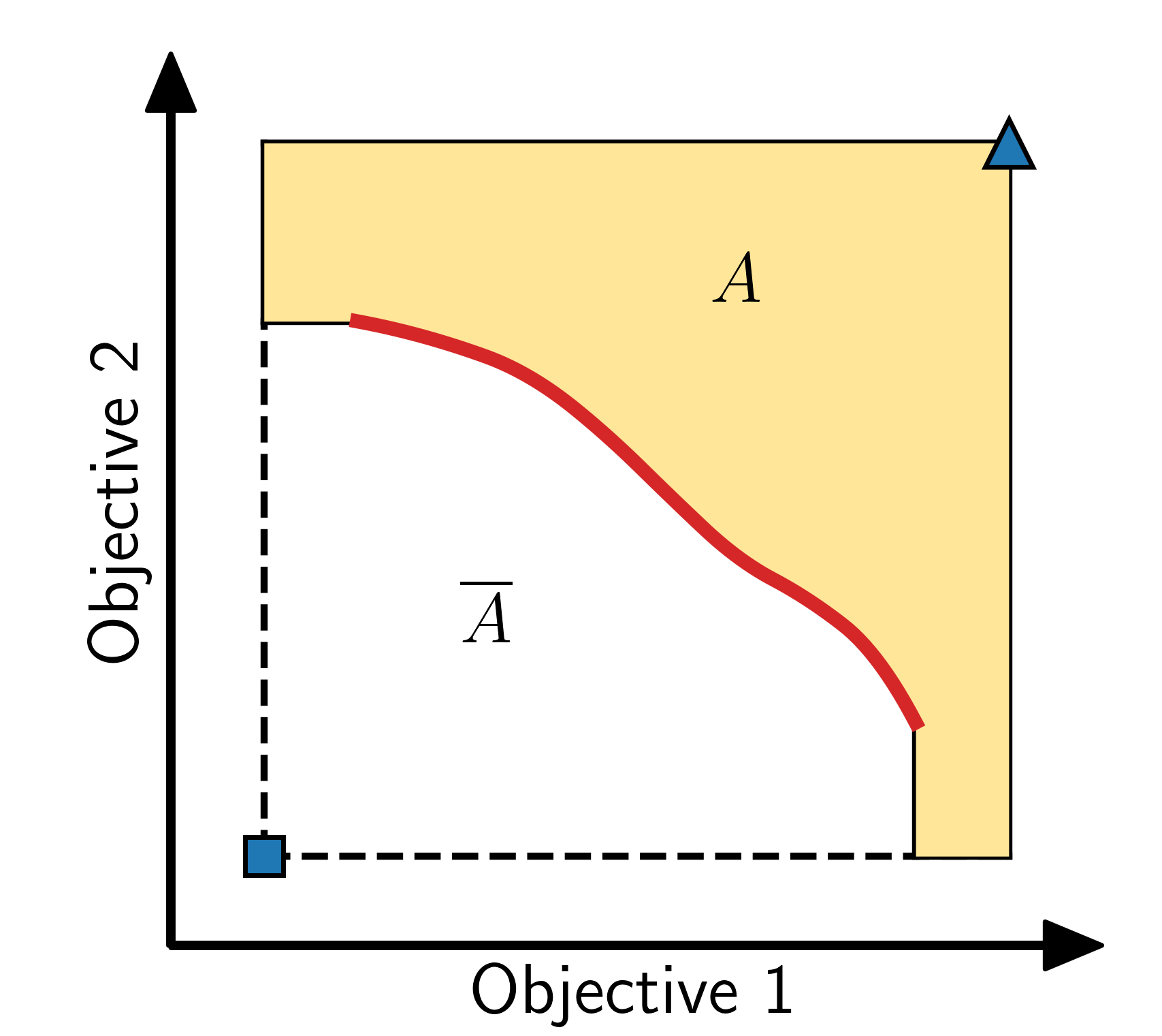
(a)

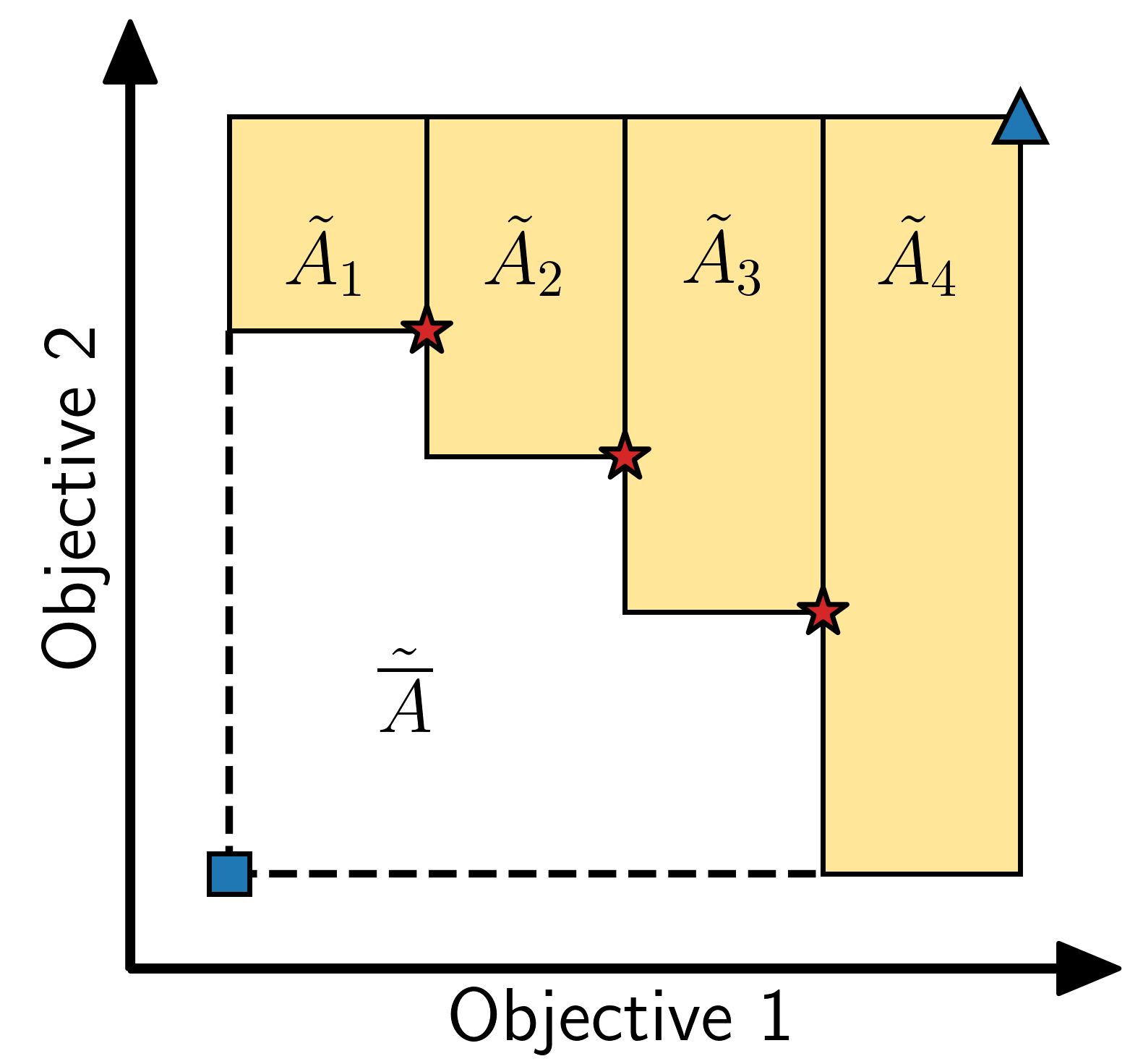
(b)

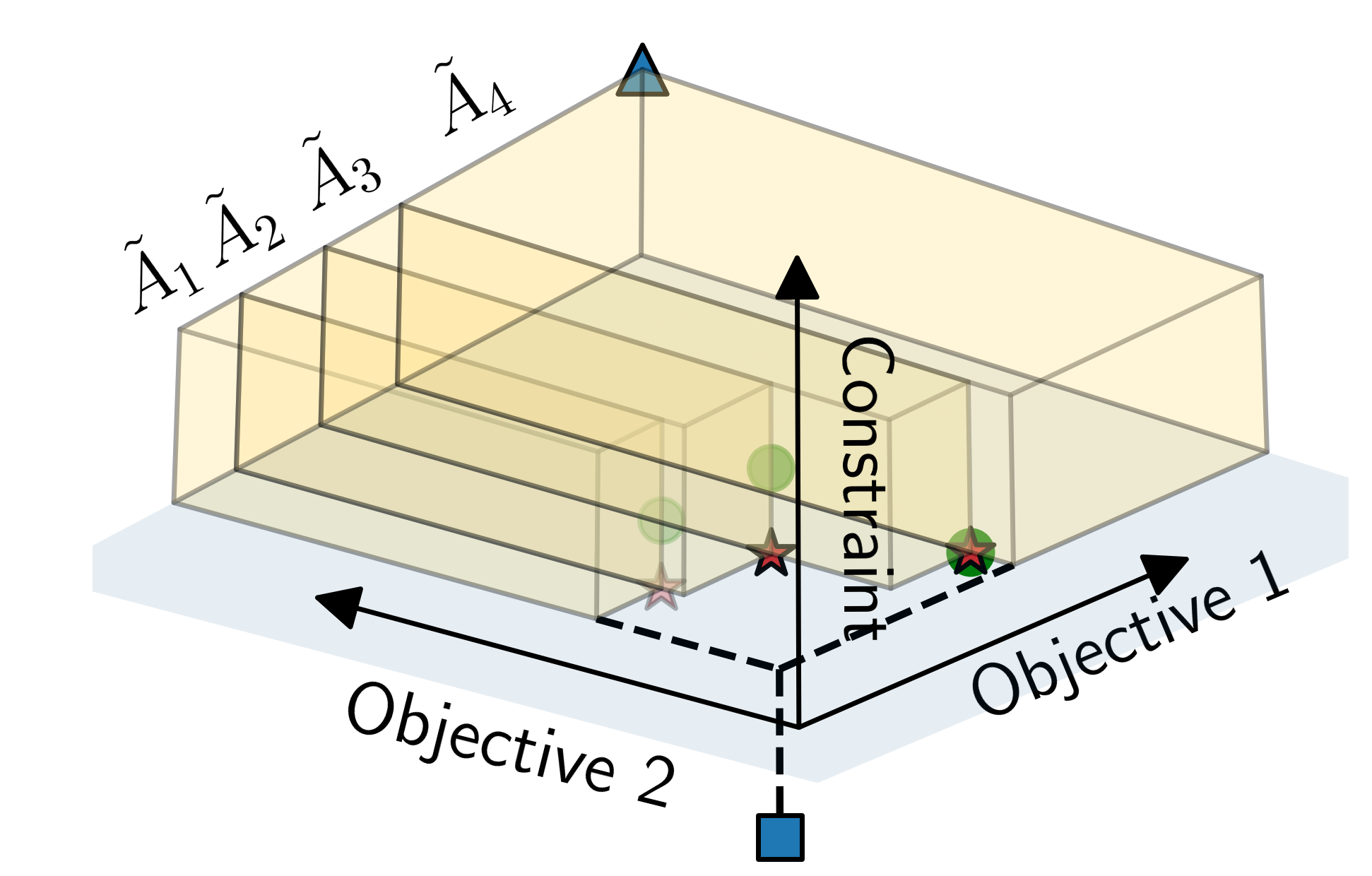
(c)

Figure 1: Partitioning the output space (bounded by the ideal point and anti-ideal point) according to a Pareto frontier: a) Given $\mathcal{F}$: Partitioning into a dominated region $\overline{A}$ and an non-dominated region $A$. b) Given a discrete Pareto frontier approximation $\tilde{\mathcal{F}}$: Partitioning the output space into an approximated dominated region $\tilde{\overline{A}}$ and non-dominated region $\tilde{A}$ by hypervolume based decomposition $\mathcal{P}$. c) A partition of the output space given a discretized feasible Pareto frontier $\tilde{\mathcal{F}}$ for a constrained optimization problem.

3 $\{\text{PF}\}^{2}$ES FOR CONSTRAINED MULTI-OBJECTIVE OPTIMIZATION

The goal is to determine where to sample $\bm{x}$ in order to learn as much as possible about the Pareto frontier $\mathcal{F}$? Under the information-theoretic framework, the act of learning is characterized by the Shannon mutual information $I(\cdot,\cdot)$ (Cover,, 1999) between our target quantity $\mathcal{F}$, and the possible distribution of the concatenated objective-constraint observations $\bm{h}_{\bm{x}}$ according to our GP surrogate models:

$$I(\mathcal{F};\bm{h}_{\bm{x}})$$ (3)

Current output-space methods for information-theoretic MOO (Belakaria et al.,, 2020; Suzuki et al.,, 2020) (i.e., those that seek to learn the Pareto Frontier, as discussed in Section 2.3) recast the mutual information (Eq. 3’s) as the reduction in differential entropy $\mathbb{H}$ of $\mathcal{F}$ provided by the candidate evaluation, i.e., using the expansion $I(\mathcal{F},\bm{h}_{\bm{x}})=\mathbb{H}(\mathcal{F})-\mathbb{H}(\mathcal{F}|\bm{h}_{\bm{x}})$. Following this formulation, the primary difficulty is providing a reliable and efficient approximation of the differential entropy $\mathbb{H}(\mathcal{F}|\bm{h}_{\bm{x}})$.

3.1 A Variational Lower Bound of the Mutual Information $I(\mathcal{F};\bm{h}_{\bm{x}})$

For $\{\text{PF}\}^{2}$ES we avoid the difficulties of approximating the differential entropy by directly approximating the mutual information itself (Eq. 3). In particular, we follow the ideas of (Poole et al.,, 2019; Takeno et al.,, 2022) and replace the mutual information with the following variational lower bound:

$$I(\mathcal{F};\bm{h}_{\bm{x}})$$ (4)

$$=\int_{\mathcal{F}}\int_{\bm{h}_{\bm{x}}}p(\bm{h}_{\bm{x}},\mathcal{F})\text{log}\frac{p(\bm{h}_{\bm{x}},\mathcal{F})}{p(\bm{h}_{\bm{x}})p(\mathcal{F})}d\mathcal{F}d\bm{h}_{\bm{x}}$$

$$=\mathbb{E}_{\mathcal{F}}\left[\int_{\bm{h}_{\bm{x}}}p(\bm{h}_{\bm{x}}|\mathcal{F})\text{log}\frac{p(\bm{h}_{\bm{x}}|\mathcal{F})q(\bm{h}_{\bm{x}}|\mathcal{F})}{p(\bm{h}_{\bm{x}})q(\bm{h}_{\bm{x}}|\mathcal{F})}d\bm{h}_{\bm{x}}\right]$$

$$=\mathbb{E}_{\mathcal{F}}\Big{[}\int_{\bm{h}_{\bm{x}}}p(\bm{h}_{\bm{x}}|\mathcal{F})\text{log}\frac{q(\bm{h}_{\bm{x}}|\mathcal{F})}{p(\bm{h}_{\bm{x}})}d\bm{h}_{\bm{x}}+$$

$$\quad\quad\quad D_{KL}(p(\bm{h}_{\bm{x}}|\mathcal{F})||q(\bm{h}_{\bm{x}}|\mathcal{F}))\Big{]}$$

$$\geq\mathbb{E}_{\mathcal{F}}\left[\int_{\bm{h}_{\bm{x}}}p(\bm{h}_{\bm{x}}|\mathcal{F})\text{log}\frac{q(\bm{h}_{\bm{x}}|\mathcal{F})}{p(\bm{h}_{\bm{x}})}d\bm{h}_{\bm{x}}\right]$$

where $D_{KL}$ represents the KL-divergence and the density $q(\bm{h}_{\bm{x}}|\mathcal{F})$ is a variational approximation of the ground truth conditional distribution $p(\bm{h}_{\bm{x}}|\mathcal{F})$. The inequality in the final line of Eq. 4 is due to the non-negativity of the KL-divergence. As the gap between the true mutual information and our lower bound can be explicitly seen as the KL-divergence between the variational approximation and ground truth conditional distribution, the suitability of this lower bound depends on our ability to build a reasonable approximation $q(\bm{h}_{\bm{x}}|\mathcal{F})\approx p(\bm{h}_{\bm{x}}|\mathcal{F})$.

We now explain how to build an effective variational approximation $q(\bm{h}_{\bm{x}}|\mathcal{F})$. Given a realization of the Pareto frontier $\mathcal{F}$ (illustrated in Fig. 1(a) for an unconstrained problem), the output space $\mathbb{R}^{M+C}$ can be partitioned into two complementary regions $A(\mathcal{F})$ and $\overline{A}(\mathcal{F})$, i.e., $A(\mathcal{F})\cup\overline{A}(\mathcal{F})=\mathbb{R}^{M+C}$ , where $A(\mathcal{F})\subset\mathbb{R}^{M+C}$ is the feasible non-dominated region $\{\{\bm{f}_{\bm{x}},\bm{g}_{\bm{x}}\}:\nexists\bm{x}^{*}\in\bm{x}_{\mathcal{F}}\ s.t.\ \bm{f}_{\bm{x}^{*}}\succ\bm{f}_{\bm{x}},\ \bm{g}_{\bm{x}}\geq\bm{0}\}$ in the output space. We then set $q(\bm{h}_{\bm{x}}|\mathcal{F})$ as (an extension of the concept of Pareto frontier truncated normal distribution (Suzuki et al.,, 2020)):

$$q(\bm{h}_{\bm{x}}|\mathcal{F})=\left\{\begin{aligned} &\frac{p(\bm{h}_{\bm{x}})}{Z_{\overline{A}}}\quad\bm{h}_{\bm{x}}\in\overline{A}\\ &0\quad\quad\quad\ \text{else}\\ \end{aligned}\right.$$ (5)

where $Z_{\overline{A}}:=\int_{\overline{A}}p(\bm{h}_{\bm{x}})d\bm{h}_{\bm{x}}=1-Z_{A}$ is the probability of $\bm{h}_{\bm{x}}$ be in $\overline{A}$, which is constructed based on the frontier realization $\overline{A}(\mathcal{F})$ . The choice of variational approximation $q$ is motivated by that, given a fixed $\mathcal{F}$, for any $\bm{x},\bm{h_{x}}$; we assign $q(\bm{h_{x}}|\mathcal{F})=0$ for $\bm{h_{x}}$ to be feasible and non-dominated (i.e., there exists $\bm{x}^{\prime}\in\bm{x}_{\mathcal{F}}$ such that $\bm{f_{x}}\succ\bm{f(x^{\prime})}$ and $\bm{g_{x}>0}$). This of course assumes that we are able to obtain the expensive observations without noise which is a common scenario (e.g., (Vakili et al.,, 2020)).

By substituting our approximate conditional distribution (Eq. 5) into Eq. 4, the variational information lower bound has the following simple expression

$$I(\mathcal{F};\bm{h}_{\bm{x}}) \geq\mathbb{E}_{\mathcal{F}}\left[\int_{\bm{h}_{\bm{x}}\in\overline{A}(\mathcal{F})}p(\bm{h}_{\bm{x}}|\mathcal{F})d\bm{h}_{\bm{x}}\cdot\text{log}\frac{1}{Z_{\overline{A}(\mathcal{F})}}\right]$$ (6)

$$=-\mathbb{E}_{\mathcal{F}}\left[\text{log}\left(1-Z_{A(\mathcal{F})}\right)\right]=\alpha_{\text{\{PF\}}^{2}\text{ES}}.$$

which leads to the proposed {PF}²ES acquisition function.

Explainability of {PF}²ES: Given the {PF}²ES’s expression in Eq. 6, we are able to link it with the common Multi-Objective Probability of Improvement (MOPI) (Yang et al.,, 2019; Hawe and Sykulski,, 2007). MOPI is the multi-objective version of Probability of Improvement (Kushner,, 1964) and measures utility by the probability that a new candidate will locate in the non-dominated region $A(\mathcal{F})$, which can be constructed based on a Pareto frontier $\mathcal{F}$. MOPI can be adapted to the CMOO setting, where it can be multiplied with a Probability of Feasibility (PoF) term ($\alpha_{MOPI}\times\alpha_{PoF}$) following the approach of (Hawe and Sykulski,, 2008; Gardner et al.,, 2014). This, under the assumption that $\bm{f}$ and $\bm{g}$ is statistically independent, is equivalent to the probability that a new candidate is feasible and located in the non-dominated region.

The link between {PF}²ES and MOPI can be established through the following remark (see Appendix. A for proof):

Remark 1.

The following acquisition functions lead to the same maximal candidate $\bm{x}=arg\ \underset{\bm{x}\in\mathcal{X}}{max}\ \alpha(\bm{x})$:

1. MOO

   1. $\alpha_{MOPI}$ using $\mathcal{F}$ as Pareto frontier

   2. $\alpha_{\{\text{PF}\}^{2}\text{ES}}$ with $|\tilde{\mathbf{F}}|=1$ and use the same $\mathcal{F}$ as 1.1.

2. Constrained MOO when

   1. $\alpha_{MOPI}$ $*$ $\alpha_{PoF}$ using $\mathcal{F}$ as reference Pareto frontier

   2. $\alpha_{\{\text{PF}\}^{2}\text{ES}}$ with $|\tilde{\mathbf{F}}|=1$ and use the same $\mathcal{F}$ as 2.1.

where $\tilde{\mathbf{F}}$ is defined in Eq. 8. We note this linkage provides insights into the empirical performance of $\{\text{PF}\}^{2}$ES as well.

4 PRACTICAL CALCULATION OF $\{\text{PF}\}^{2}$ES AND ITS PARALLELIZATION

Practical calculation of the variational lower bound (Eq. 6) requires some additional steps. The primary difficulty is that the region $A$ (for any given Pareto frontier $\mathcal{F}$) does not have an analytical form. A popular approach (Belakaria and Deshwal,, 2019; Suzuki et al.,, 2020; Hernández-Lobato et al.,, 2016; Garrido-Merchán and Hernández-Lobato,, 2019) is to use a finite representation of the Pareto frontier $\tilde{\mathcal{F}}$:= $\{\bm{f}|\bm{f}\in\mathcal{F}\}\ s.t.\ |\tilde{\mathcal{F}}|<\infty$. Based on $\tilde{\mathcal{F}}$, a hypervolume-based output space partitioning strategy (Lacour et al.,, 2017; Couckuyt et al.,, 2012), denoted as $\mathcal{P}$, can be used to partition the output space into $N_{p}$ disjoint hypercubes, thus obtaining an approximation of $A$ denoted by hypervolume based approximated non-dominated region:

$$A\approx\tilde{A}(\tilde{\mathcal{F}})=\mathcal{P}(\tilde{\mathcal{F}})=\{\tilde{A}_{1},\tilde{A}_{2},...,\tilde{A}_{N_{p}}\}$$ (7)

which is the complement of $\tilde{\overline{A}}(\tilde{\mathcal{F}}):=\{\bm{f}_{\bm{x}}\in\mathbb{R}^{M}|\exists\bm{f}\in\tilde{\mathcal{F}},\bm{f}_{\bm{x}}\preceq\bm{f}\}$. Such partitioning is illustrated in Fig. 1(b) for unconstrained MOO problems. For CMOO problem, $\tilde{A}(\tilde{\mathcal{F}})$ can be obtained by first partitioning the non-dominated region in the objective space: $\mathbb{R}^{M}$ and then concatenated with the constraint space where $\bm{g}\geq\bm{0}$, see Fig. 1(c) for an illustration.

Given $\tilde{A}$, we are able to reach the following analytically tractable approximation of Eq. 6:

$$-\mathbb{E}_{\mathcal{F}}\left[\text{log}\left(1-Z_{A(\mathcal{F})}\right)\right]\approx-\frac{1}{|\tilde{\mathbf{F}}|}\sum_{\tilde{\mathcal{F}}\in\tilde{\mathbf{F}}}\left[\text{log}\left(1-\sum_{i=1}^{N_{p}}Z_{{\tilde{A}}_{i}}\right)\right]$$ (8)

where $\tilde{\mathbf{F}}$ is a set of sampled Pareto frontiers providing a Monte Carlo (MC) approximation of the outer expectation in Eq. 6. We build this MC sample of $\tilde{\mathcal{F}}$ by using a standard multi-objective optimization algorithm (e.g., NSGAII (Deb et al.,, 2002)) on samples from the GP’s spectral posterior (also known as sampling GP posterior via its Fourier features (Rahimi and Recht,, 2007)), which is a common strategy utilized in acquisition functions for MOO (Belakaria and Deshwal,, 2019; Suzuki et al.,, 2020; Daulton et al.,, 2022). $Z_{\tilde{A}_{i}}$ is the probability that $\bm{h}_{\bm{x}}$ is in the $i^{\prime}$th hypercube $\tilde{A}_{i}$ and can be calculated as (Suzuki et al.,, 2020):

$$Z_{\tilde{A}_{i}}=\prod_{k=1}^{M+C}\left(\Phi(\frac{\tilde{A}_{i_{u}}^{k}-\bm{m}_{\bm{x}}^{k}}{\bm{\sigma}_{\bm{x}}^{k}})-\Phi(\frac{\tilde{A}_{i_{l}}^{k}-\bm{m}_{\bm{x}}^{k}}{\bm{\sigma}_{\bm{x}}^{k}})\right).$$ (9)

where $\Phi(\cdot)$ represents the cumulative density function of the standard normal distribution, $\tilde{A}_{i_{u}}^{k},\tilde{A}_{i_{l}}^{k}$ represents the $k^{\prime}$th dimensional upper and lower bound of the $i^{\prime}$th hypercube, respectively. $\bm{m}_{\bm{x}}^{k},\bm{\sigma}_{\bm{x}}^{k}$ represent the $k^{\prime}$th dimensional GP posterior mean and standard deviation, respectively.

Unfortunately, due to the subtlety of our employed partitioning strategy, we cannot simply use the r.h.s of Eq. 8 as $\alpha_{\{\text{PF}\}^{2}\text{ES}}$. In particular, the hyper-volume based partition $\mathcal{P}$, operating on the finite representation $\tilde{\mathcal{F}}$, means that $\tilde{A}$ is an overestimation of the non-dominated region $A$. Therefore, we are no longer guaranteed to satisfy the lower bound property in Eq. 6 since $Z_{A(\mathcal{F})}<Z_{A(\tilde{\mathcal{F}})}$. More importantly, calculating {PF}²ES based on the above $\tilde{A}$ results in the same empirical clustering issue observed in MOPI, i.e. that the probability of improvement rewards tiny improvements of the Pareto frontier approximation $\tilde{\mathcal{F}}$ if they are achieved with high confidence (Emmerich et al.,, 2020) (see Appendix. B for a detailed elaboration).

In order to mitigate this clustering issue whilst ensuring that our acquisition function remains true to its motivation as a lower bound to the mutual information, we propose a small change to how we construct our approximation of $A$. Inspired by the common empirical strategy employed in MOPI and PI acquisition functions ((Wang et al.,, 2016; Emmerich et al.,, 2020; Kushner,, 1964)), we introduce a small positive penalization vector $\bm{\varepsilon}=[\varepsilon_{1},...,\varepsilon_{M}]$ to shift the discrete Pareto frontier approximation:$\tilde{\mathcal{F}_{\bm{\varepsilon}}}:=\tilde{\mathcal{F}}+\bm{\epsilon}$ to avoid any overestimation of $A$ resulting from the hyper-volume decomposition. In Appendix. D, we show that it is possible to construct an $\epsilon$ that ensures that our acquisition function remains a lower bound. However, building such an epsilon is costly, so we also propose the practical solution of setting $\epsilon$ through a simple heuristic that achieves very similar empirical performance (see Appendix. D). In particular, we set epsilon as $\epsilon_{k}=c\left(max(\tilde{\mathcal{F}^{k}})-min(\tilde{\mathcal{F}^{k}})\right)$ $\forall k\in M,\tilde{\mathcal{F}}\in\tilde{\mathbf{F}}$. i.e. a proportion of the maximal total variation observed over the Pareto front. We show empirically that {PF}²ES’s performance is robust to the choice of $c$ through sensitivity analysis (Appendix. F). We set $c=0.04$ for all our experiments.

Combining all these steps, we can finally state our proposed acquisition function as

$$\tilde{\alpha}_{\{\text{PF}\}^{2}\text{ES}}=-\frac{1}{|\tilde{\mathbf{F}}|}\sum_{\tilde{\mathcal{F}}\in\tilde{\mathbf{F}}}\left[\text{log}\left(1-\sum_{i=1}^{N}Z_{{\tilde{A}}_{i}(\mathcal{F}_{\varepsilon})}\right)\right].$$ (10)

See Algorithm 1 in Appendix. D for a high-level algorithmic summary of our calculation strategy.

4.1 Parallelisation of $\{\text{PF}\}^{2}$ES

For many practical MOO problems, it is common to have parallel or distributed evaluation resources available, i.e. we recommend $q>1$ evaluations during each BO step. We now propose an extension of $\{\text{PF}\}^{2}$ES that allows it to be used for such batch optimizations. This time, the principled question is at which $q$ points should we sample simultaneously to learn as much as possible about $\mathcal{F}$?

Consider the random variable $\bm{h}_{\bm{X}}=\{\bm{h}_{\bm{x}_{1}},...,\bm{h}_{\bm{x}_{q}}\}$, i.e., the possible observations that could arise from a parallel evaluation of a batch of $q$ points. In this scenario, we want to allocate a batch of $q$ points X that provide the most mutual info about the (feasible) Pareto frontier. Following the same derivation as Eq. 4 - 6, we are able to have our proposed extension of $\{\text{PF}\}^{2}$ES for batch design:

$$\tilde{\alpha}_{\text{q-}\{\text{PF}\}^{2}\text{ES}}\approx-\frac{1}{|\tilde{\mathbf{F}}|}\sum_{\tilde{\mathcal{F}}\in\tilde{\mathbf{F}}}\left[\text{log}\left(1-Z_{\tilde{A}_{q}(\tilde{\mathcal{F}}_{\bm{\varepsilon}})}\right)\right],$$ (11)

where $Z_{\tilde{A}_{q}}:=\int_{\tilde{A}_{q}}p(\bm{h}_{\bm{X}})d\bm{h}_{\bm{X}}$ see Eq. 17). i.e., the probability that there exists at least one batch element $\bm{h}_{\bm{x}_{i}}\in\bm{h}_{\bm{X}}$ such that $\bm{h}_{\bm{x}_{i}}\in\tilde{A}(\tilde{\mathcal{F}}_{\bm{\varepsilon}})=\{\tilde{A}_{1}(\tilde{\mathcal{F}}_{\bm{\varepsilon}}),...,\tilde{A}_{N}(\tilde{\mathcal{F}}_{\bm{\varepsilon}})\}$. Calculating the probability of $Z_{\tilde{A}}$ involves a complex interaction between joint batch points within the complex region $\tilde{A}$; we hence propose to approximate this probability through an MC approximation (a detailed derivation is provided in Appendix. C.1):

$$Z_{\tilde{A}_{q}}$$ (12)

$$\approx\frac{1}{N_{MC}}\sum_{j=1}^{N_{MC}}\left(\bigcup_{i=1}^{N_{p}}\left(\bigcup_{l=1}^{q}\left(\prod_{k=1}^{M+C}\left(\mathbbm{1}(A_{i_{l}}^{k}\leq\bm{h}_{\bm{x}_{l_{j}}}^{k}\leq A_{i_{u}}^{k})\right)\right)\right)\right)$$

$$\approx\frac{1}{N_{MC}}\sum_{j=1}^{N_{MC}}\left(max_{i}\left(max_{l}\left(\prod_{k=1}^{M+C}\left(\sigma(\frac{\bm{h}_{\bm{x}_{l_{j}}}^{k}-A_{i_{l}}^{k}}{\tau})\cdot\right.\right.\right.\right.$$

$$\left.\left.\left.\left.\quad\sigma(\frac{A_{i_{u}}^{k}-\bm{h}_{\bm{x}_{l_{j}}}^{k}}{\tau})\right)\right)\right)\right),$$

where $\bm{h}_{{\bm{x}_{l}}_{j}}^{k}$ represents the $k^{\prime}$th output dimensionality of $j^{\prime}$th MC sample of $l^{\prime}$th batch point $\bm{h}_{{\bm{x}_{l}}}$, and $\sigma(\cdot)$ is the sigmoid function, $N_{MC}$ represents the MC sample size. To ensure the differentiability of our acquisition function, we follow a common strategy in BO (Wilson et al.,, 2018; Daulton et al.,, 2020) to relax the categorical event imposed by $\mathbbm{1}(\cdot)$ in the first line of Eq. 12 by replacing it with a sigmoid function and a small non-negative temperature parameter $\tau$. We note Eq. 12 can be explained as calculating the event that whether any batch element is within $\tilde{A}$, averaged through $N_{MC}$ sample numbers. For joint sampling of the batch outcome $\bm{h}_{\bm{X}}$, we use the reparameterization trick in combination with a sample average approximation (SAA) (Balandat et al.,, 2020) to perform a continuous acquisition function optimization process, where the base sample of SAA has been generated through a randomized quasi-Monte Carlo ( details of the approximation and a demonstration of q-{PF}²ES is provided in Appendix. C.2).

We stress the existence of remark. 1 confirms that our MC-based parallelisation strategy (Eq. 12) can be directly applied to the MOPI acquisition function as well.

Complexity Analysis Lastly, we provide complexity analysis in Appendix G, A run-time comparison with other acquisition functions utilized in the next section is also conducted and detailed in Appendix H.

5 EXPERIMENTAL VALIDATION OF $\{\text{PF}\}^{2}$ES

We now present the empirical performance of $\{\text{PF}\}^{2}$ES across constrained and unconstrained synthetic benchmarks and real-life application problems. The primary focus of these experiments is to compare our methods with other output-based entropy search methods, we have also included the golden standard EHVI acquisition functions as a performance reference .

Sequential MOO problem We compare against PFES (Suzuki et al.,, 2020), MESMO (Belakaria et al.,, 2020), EHVI (Yang et al.,, 2019), PESMO (Hernández-Lobato et al.,, 2016), as well as providing random search as a common baseline.

Parallel MOO problem We compare against qEHVI (Daulton et al.,, 2020), {PF}²ES with a fantasizing method (i.e., the Kriging Believer (KB) method (Ginsbourger et al.,, 2010)) and random search.

Sequential CMOO problem We compare against EHVI-PoF (the multiplication of EHVI with PoF as a common strategy for CMOO (e.g., Martínez-Frutos and Herrero-Pérez, (2016))), MESMOC (Belakaria et al.,, 2021), MESMOC+ (Fernández-Sánchez et al.,, 2020) and random search.

Parallel CMOO problem We compare against qEHVI (Daulton et al.,, 2020), PPESMOC (Garrido-Merchán and Hernández-Lobato,, 2020), random Search and {PF}²ES using a fantasize method (Ginsbourger et al.,, 2010).

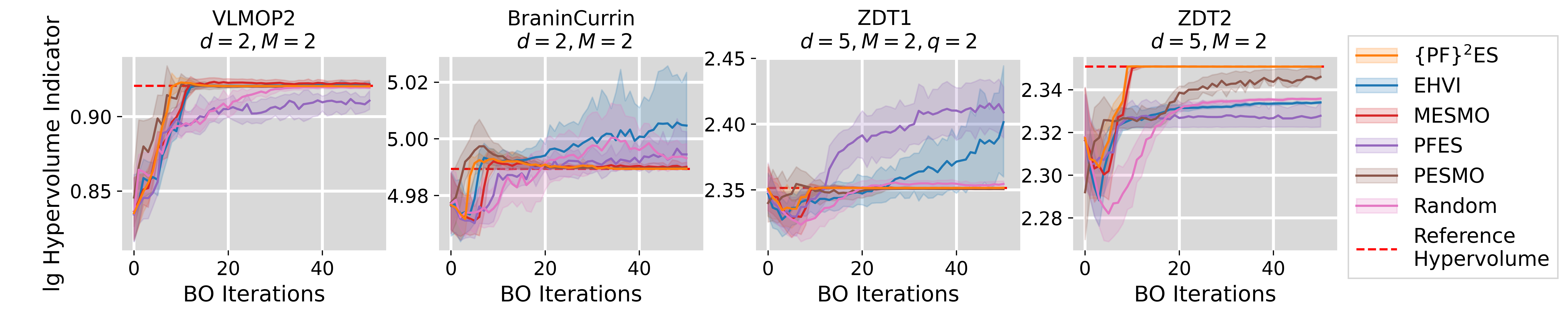
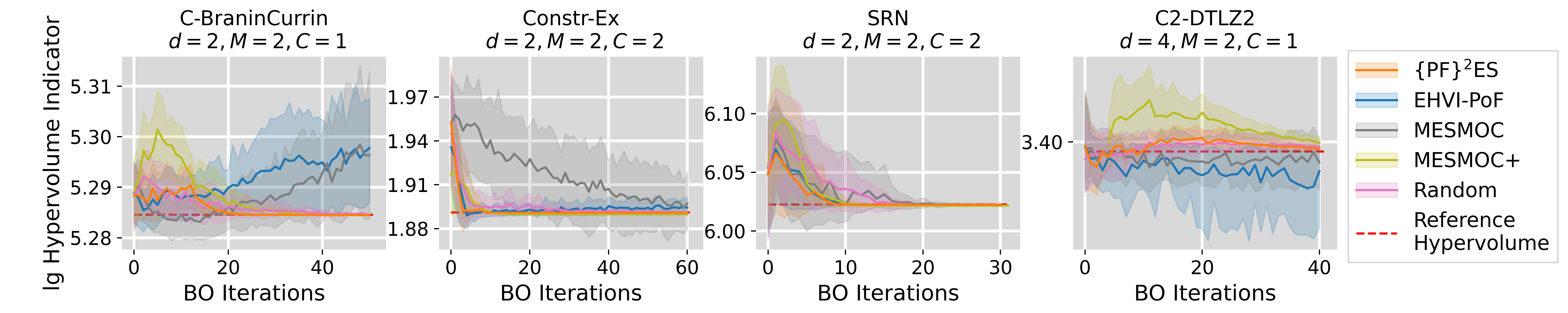
Figure 2: Uncertainty Calibration of inferred Pareto Frontier during BO iterations.

For PESMO, MESMOC+ and PPESMOC, we used the public implementation provided by the papers. The settings of all acquisition functions are detailed in Appendix. E.3. For the surrogate models, we build GPs with Matérn 5/2 kernels using maximum a posteriori estimates for the kernel parameters. For optimizing the acquisition functions, we use a multi-start L-BFGS-B optimizer starting from the $min(10\times qd,100)$ best locations from 5000 random starting locations. For the hyperparameter of the acquisition function, we empirically choose $\tau=1e-3$ . For sampling the (feasible) Pareto frontier $\tilde{\mathcal{F}}$, we use the open-source NSGAII optimizer in PyMOO (Blank and Deb,, 2020), where constraints are handled by the parameter-less approach (Deb and Agrawal,, 1999). For all our information-theoretic acquisition functions, we use five sampled Pareto frontiers. All of the following experiments start with $2d+1$ random sampled initial points. For the recommendation of optimal candidates, we use the out-of-sample strategy (performing recommendation based on the GP model) as a common approach in the information-theoretic acquisition function (see Appendix. E.2 for details).

First, we consider a suite of popular synthetic benchmarks. Details of the benchmark functions, the reference point settings, and benchmark results on in-sample recommendations are provided in Appendix. E.1, I.1 respectively.

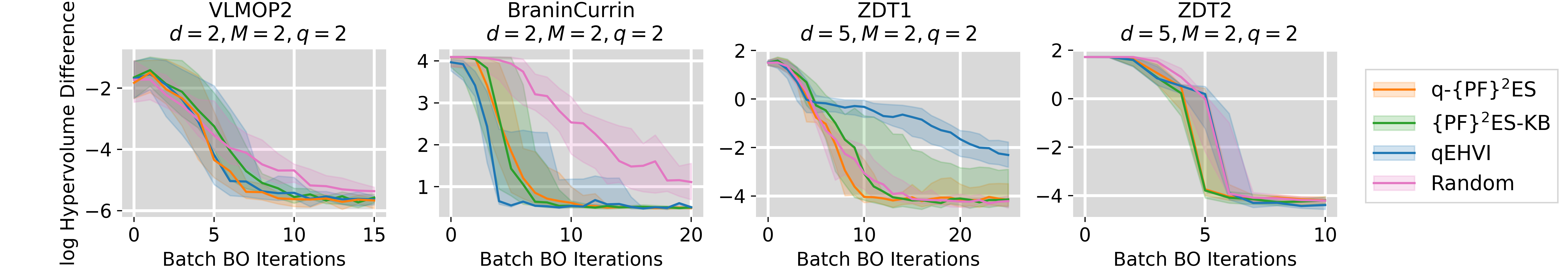
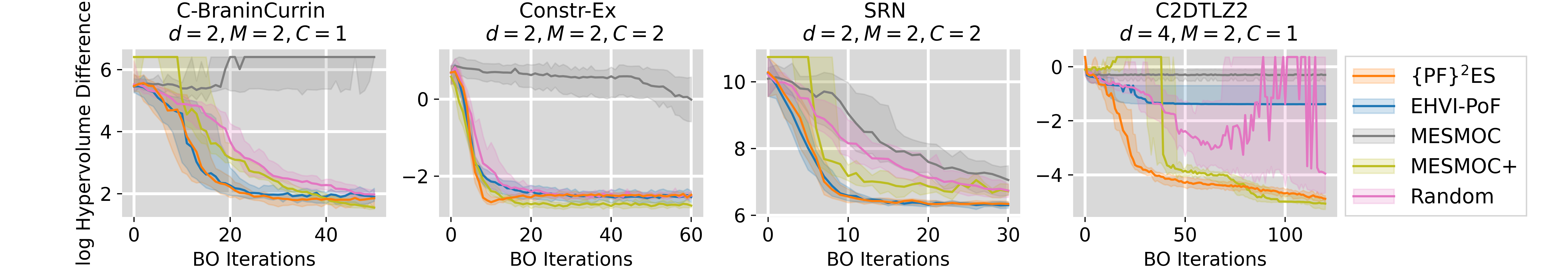
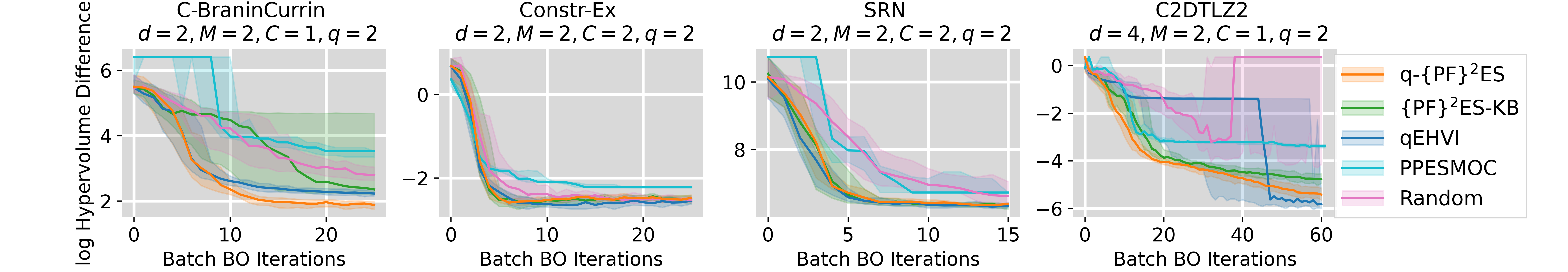
Figure 3: Comparison of different acquisition functions for multi-objective Bayesian optimization. Results are shown through median performances and interquartile ranges.

5.1 Uncertainty Calibration of Inferred Pareto Frontier

To help discern between {PF}²ES and other information-theoretic acquisition functions that choose points with the overarching goal of reducing uncertainty in the Pareto frontier, it is natural to include a performance metric that directly measures this property.

Therefore, inspired by an approach in active learning (Qing et al.,, 2021), we propose an uncertainty calibration procedure on a hypervolume based Pareto frontier indicator distribution that reflects the uncertainty of GPs w.r.t the Pareto frontier. More specifically, the hypervolume indicator function $I(\cdot)$ (Guerreiro et al.,, 2020) is applied to each sampled Pareto frontier $\tilde{\mathcal{F}}$ from the GPs. This way, a one-dimensional distribution of hypervolume indicators is obtained. Note that if the sampled Pareto frontiers have converged to the (finite approximation of the) Pareto frontier $\mathcal{F}$, the distribution will collapse to the hypervolume indicator of the (finite approximation of the) Pareto frontier $\mathcal{F}$. Hence, the expectation and uncertainty of the hypervolume based Pareto frontier indicator distribution can serve as a representation of the Pareto frontier estimation accuracy as well as the uncertainty based on GPs, respectively.

The proposed uncertainty calibration metric is illustrated in Fig. 2. For each BO iteration, the Pareto frontier indicator distribution $I(\tilde{\mathcal{F}}(GP))$ is approximated by 10 MC samples of $\tilde{\mathcal{F}}$ and we present the aggregate results across 30 repetitions of experiments by their median and 10-90 percentile. It can be seen that {PF}²ES achieved the fastest convergence to the reference hypervolume, implying low uncertainty about the Pareto frontier indicator distribution.

5.2 Multi-Objective Bayesian Optimization

Synthetic Problems

We now present our main experimental results. The log-hypervolume difference achieved across 30 repetitions for each algorithm is reported in Fig. 3. We see that {PF}²ES leads to competitive performance in both MOO and CMOO problem in the case of sequential and batch sampling. Note that the performance of EHVI, often regarded as the gold standard, relies on setting a reasonable reference point. For problems where there is no prior information known about the reference point location, dynamic reference updating strategies must be used. For example, EHVI performs poorly on C2DTLZ2 which has disjoint Pareto frontiers (Deb,, 2019). Additional experimental results on larger batch sizes and larger output dimensionalities are provided in Appendix. I.2 and I.3 respectively.

Four BarTruss Design

We consider a real-life mechanical design problem (MOO) (Tanabe and Ishibuchi,, 2020; Dauert,, 1993), where we seek a four elastic truss structure system with small structure volume whilst having small deformation under external forces. The cross-section areas of the four bars in the truss system are chosen as the design variables for the unconstrained multi-objective optimization problem. Note the scale of the two objectives is significantly different for this problem.

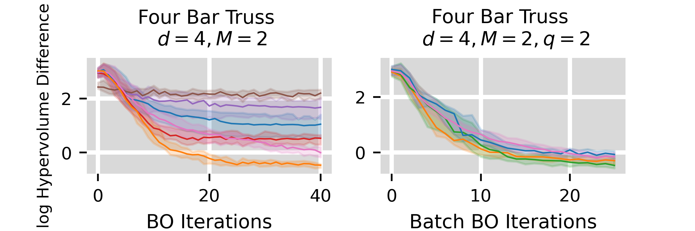
Figure 4: Four Bar Truss experimental results (with the same legend as Fig. 3).

The results are depicted in Fig. 4. For the sequential case, {PF}²ES demonstrates the overall fastest convergence speed. While all acquisition functions tend to have similar performance in the batch scenario.

Disc Brake Design Finally, we consider a real-life disc brake design problem (CMOO) (Tanabe and Ishibuchi,, 2020; Ray and Liew,, 2002). Here, the objectives are the mass of the brake and the achieved stopping time. The design variables are the inner radius and outer radius of the discs, the engaging force, and the number of friction surfaces. Four constraints are presented in this problem: the minimum distance between the radii, maximum length of the brake, pressure, temperature, and torque limitations.

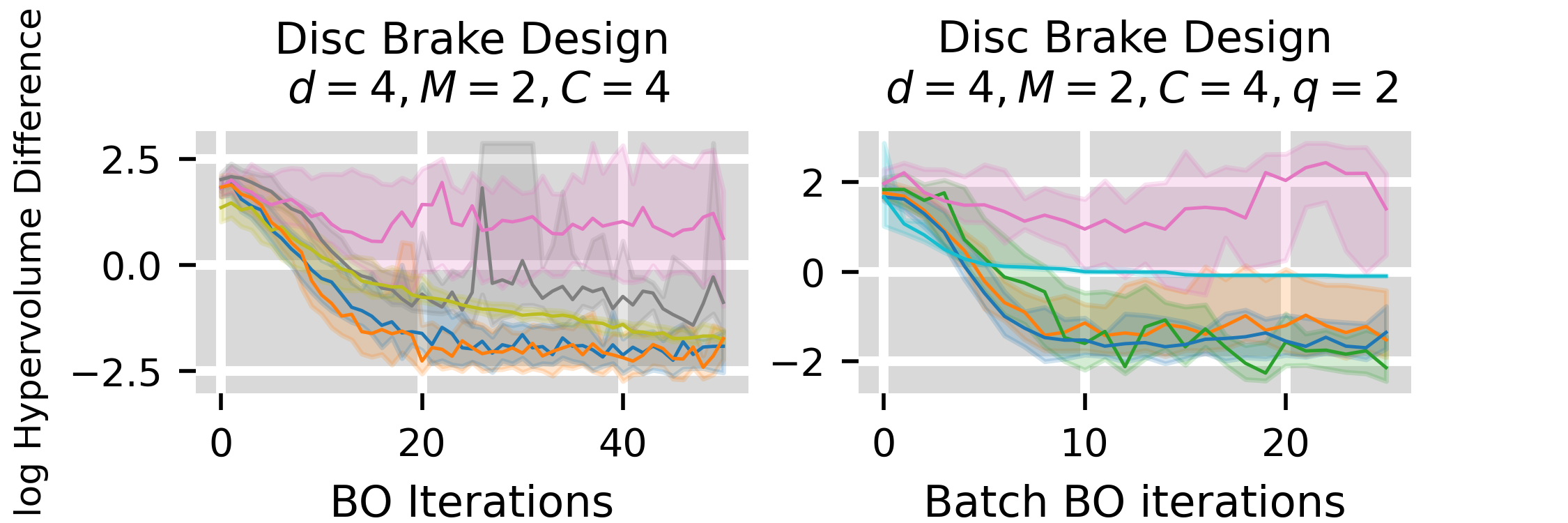
Figure 5: Disc Brake Design experimental results (with the same legend as Fig. 3).

The results are depicted in Fig. 5. {PF}²ES demonstrate the overall fast convergence speed, while {PF}²ES-KB and qEHVI are slightly better than q-{PF}²ES in terms of stable performance.

6 CONCLUSION

We have presented a new information-theoretic acquisition function $\{\text{PF}\}^{2}$ES. By using a variational lower bound to the mutual information, $\{\text{PF}\}^{2}$ES provides efficient (batch) multi-objective optimization for problems with unknown constraints. Extensive experimentation demonstrates the competitive performance of $\{\text{PF}\}^{2}$ES over other entropy-based methods. We also advocate the advantages of {PF}²ES to other greedy acquisition functions (e.g., EHVI), i.e., it is free from the requirement of a proper configuration of a reference point, which arguably is often unknown for real-life applications and can affect the performance of acquisition functions to a large extent.

Limitations and Future Work The current out-of-sample recommendation is based on the posterior mean of the GP. Hence, its performance depends on the modeling accuracy of the GP itself which means it can suffer from the curse of input dimensionality. Furthermore, the current out-of-sample recommendation strategy can be extended to a Bayesian version. Future research will focus on tackling these aspects and making the parallelization scalable to much larger batch sizes.

7 SOCIAL IMPACT

This paper presents a fundamental approach for multi-objective Bayesian Optimization and has no direct societal impact or ethical consequences. It can be used in generic real-life applications from, e.g., machine learning to engineering. Of course, the applications themselves can have an impact. As a Bayesian Optimization technique, {PF}²ES aims for identifying the Pareto frontier hopefully with less expensive black-box function evaluations (e.g., expensive biomedical experiments, power-consuming simulations), hence contributing to less energy consumption.

Appendix A RELATIONSHIP WITH THE MULTI-OBJECTIVE PROBABILITY OF IMPROVEMENT

We provide additional insights for $\{\text{PF}\}^{2}$ES by linking Eq. 6 to the Multi-objective Probability of Improvement (MOPI) (Yang et al.,, 2019). First, we define the following generic formulation of MOO acquisition functions:

$$\alpha_{MOO}=\int_{E}g\left(\int_{F}\ell(F,E)p(F)dF\right)p(E)dE,$$ (15)

where $\ell(\cdot)$ and $g(\cdot)$ are arbitrary functions, and $E$ and $F$ are random events. Evidently, $\{\text{PF}\}^{2}$ES is a special case obtained by setting $E:=\mathcal{F}$, $F:=\bm{h}_{\bm{x}}$, $\ell(\bm{h},\mathcal{F}):=\mathbbm{1}(\bm{h}_{\bm{x}}\in A(\mathcal{F}))$, and $g(\cdot):=-log(1-\cdot)$. Here $\mathbbm{1}(\cdot)$ is the indicator function.

Subsequently, by setting $\ell(E,F):=\mathbbm{1}(\bm{h}_{\bm{x}}\in\tilde{A}(\mathcal{F}))$ (i.e., $F:=\bm{h}_{\bm{x}}$ and $E:=\mathcal{F}$), $g(\cdot)$ as the identity function, and specifying a Dirac delta distribution over the Pareto frontier $\mathcal{F}$, we see that the inner integration $\int_{F}\ell(F,E)p(F)dF$ for both $\{\text{PF}\}^{2}$ES and MOPI evaluates to $p(\bm{h}_{\bm{x}}\in\tilde{A}(\mathcal{F}))$. Therefore, as $g_{\{\text{PF}\}^{2}\text{ES}}(\cdot)$ and $g_{MOPI}(\cdot)$ are both monotonic increasing over $\left(0,1\right)$, the acquisition functions have the same maximizer, i.e., where $p(\bm{h}_{\bm{x}}\in\tilde{A}(\mathcal{F}))$ is largest. The constraint case (i.e., remark 1.2) is obtained by assuming independency of $\bm{f}$ and $\bm{g}$.

Appendix B MITIGATING THE CLUSTERING ISSUE

We first demonstrate the clustering issue on the inverted VLMOP2 problem (Van Veldhuizen and Lamont,, 1999), i.e., we adopt VLMOP2 for maximization by taking the negative of each objective function. For illustrative purposes, the parameters for extracting the Pareto frontier in $\tilde{\alpha}_{\{\text{PF}\}^{2}\text{ES}}(\tilde{A}(\tilde{\mathcal{F}}))$ are set to $|\bm{\tilde{F}}|=5$ and $|\tilde{\mathcal{F}}|=5\ \forall\tilde{\mathcal{F}}\in|\bm{\tilde{F}}|$.

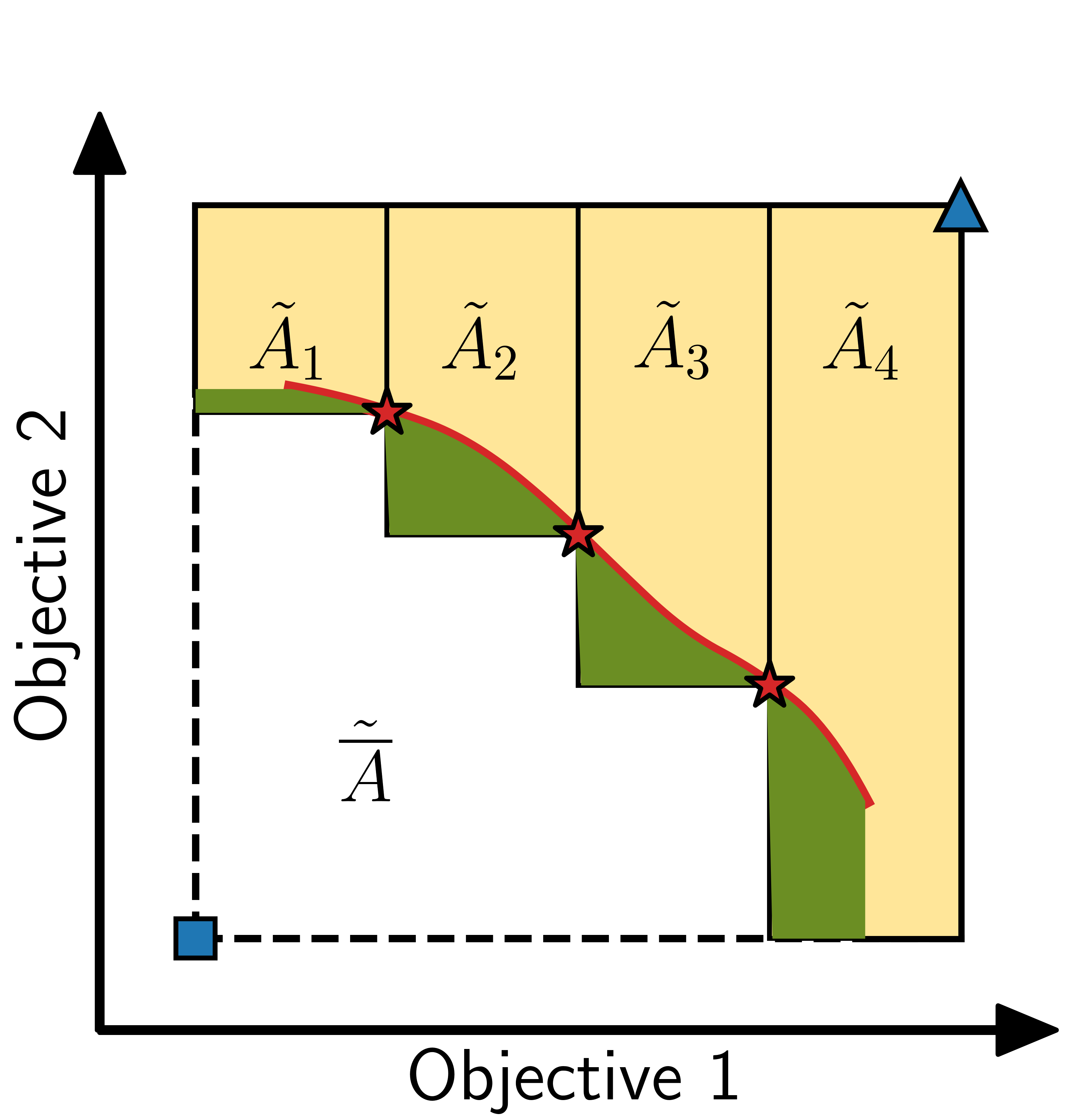
(a)

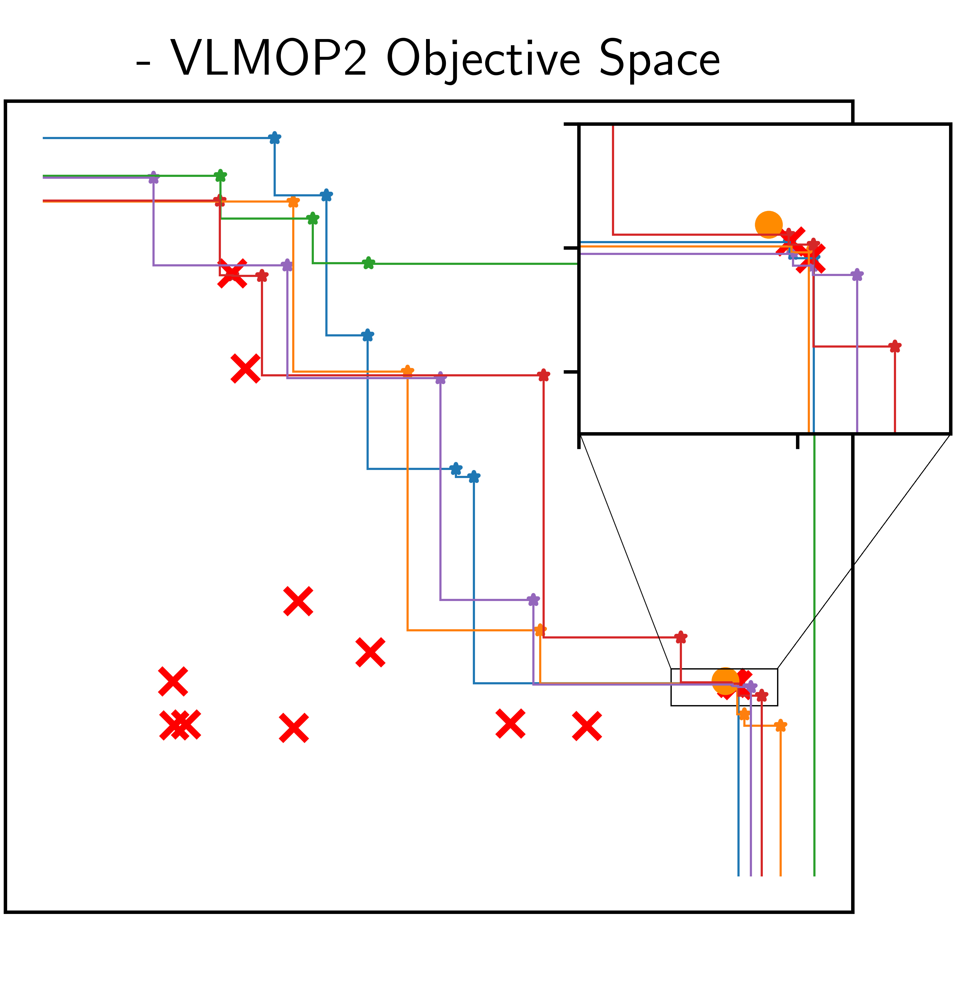
(b)

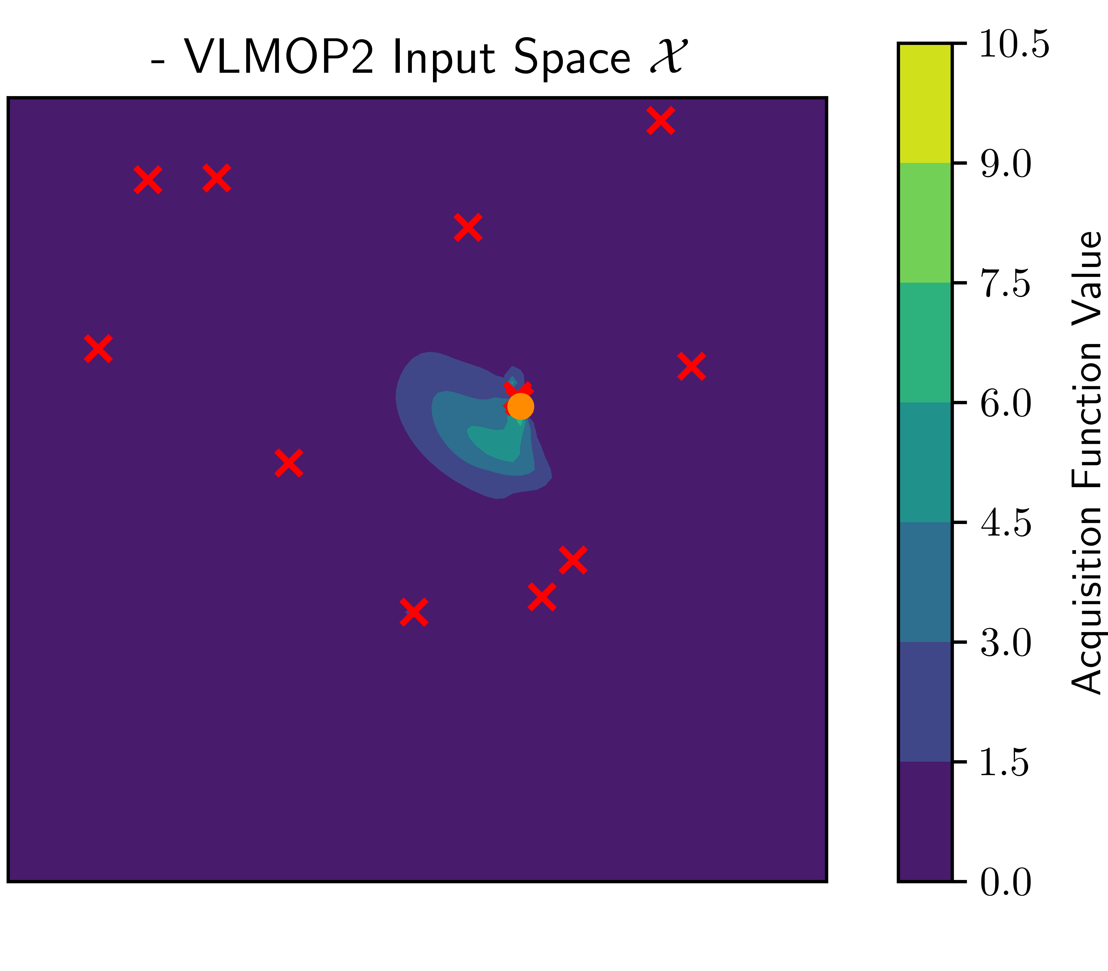
(c)

Figure 5: The hypervolume partition strategy for a discrete Pareto frontier $\tilde{\mathcal{F}}$ is an overestimation of the actual non-dominated space $A$. a) Part of the dominated region has been misclassified as non-dominated (green area). b) This overestimation will make the clustering more severe when calculating {PF}²ES based on $\tilde{A}(\tilde{\mathcal{F}})$: For a certain iteration, given the MC samples of $\tilde{\mathcal{F}}$, {PF}²ES favors the ’false positive’ location in the output space ($\bm{\sigma}_{\bm{x}}=[0.00158,0.00112]$) that is certain (high confidency) to (marginally) improve. c) This causes a clustering issue as candidates very close to existing training data points are preferred.

A contour of {PF}²ES based on the approximation of Eq. 8 is depicted in Fig. 5, which shows that the new candidate point is believed to make an improvement with high confidence (due to the small GP posterior variance) in 4 of the 5 Pareto frontier samples. Unfortunately, the improvement is marginal as the predicted observation is located in the (relatively small) false positive region introduced by the hypervolume decomposition $\mathcal{P}$, see Fig. 5(a). In practice, {PF}²ES will tend to keep sampling in a region that it is confident to make tiny (or no) improvements, causing the sampled points to be densely clustered in a small region of the input domain $\mathcal{X}$.

In order to mitigate this issue and encourage the acquisition function to focus more on where the Pareto frontier is uncertain, we utilize a parameter $\varepsilon$ to shift the Pareto frontier approximation $\mathcal{\tilde{F}}$ and shrink the false positive region. The effect is demonstrated in Fig. 6. It can be seen that the modified acquisition function $\tilde{\alpha}_{\{\text{PF}\}^{2}\text{ES}}(\tilde{A}(\tilde{\mathcal{F}}_{\varepsilon}))$ tend to be more explorative than the naive approach $\tilde{\alpha}_{\{\text{PF}\}^{2}\text{ES}}(\tilde{A}(\tilde{\mathcal{F}}))$ (i.e., based on Eq. 8).

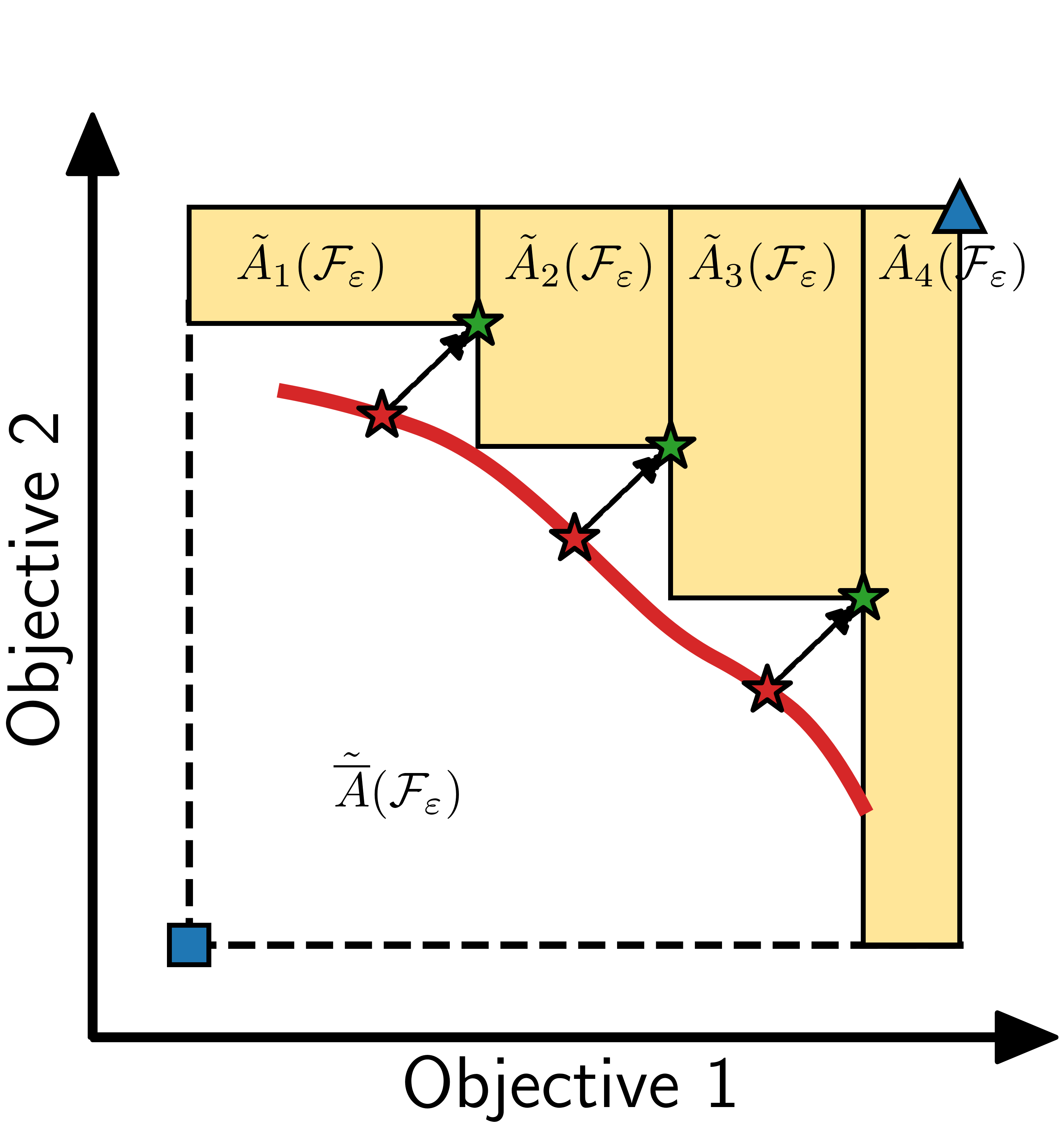
(a)

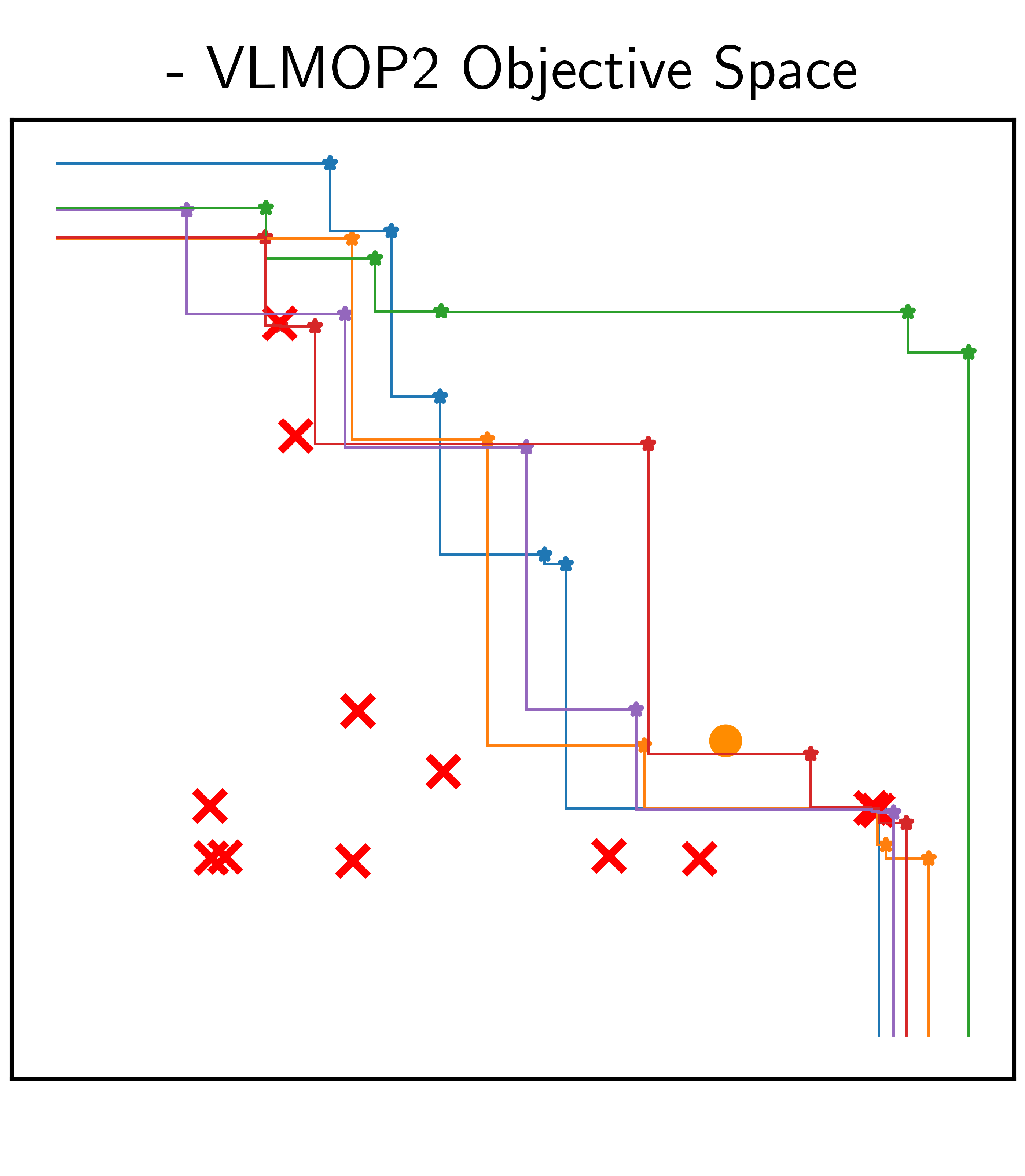
(b)

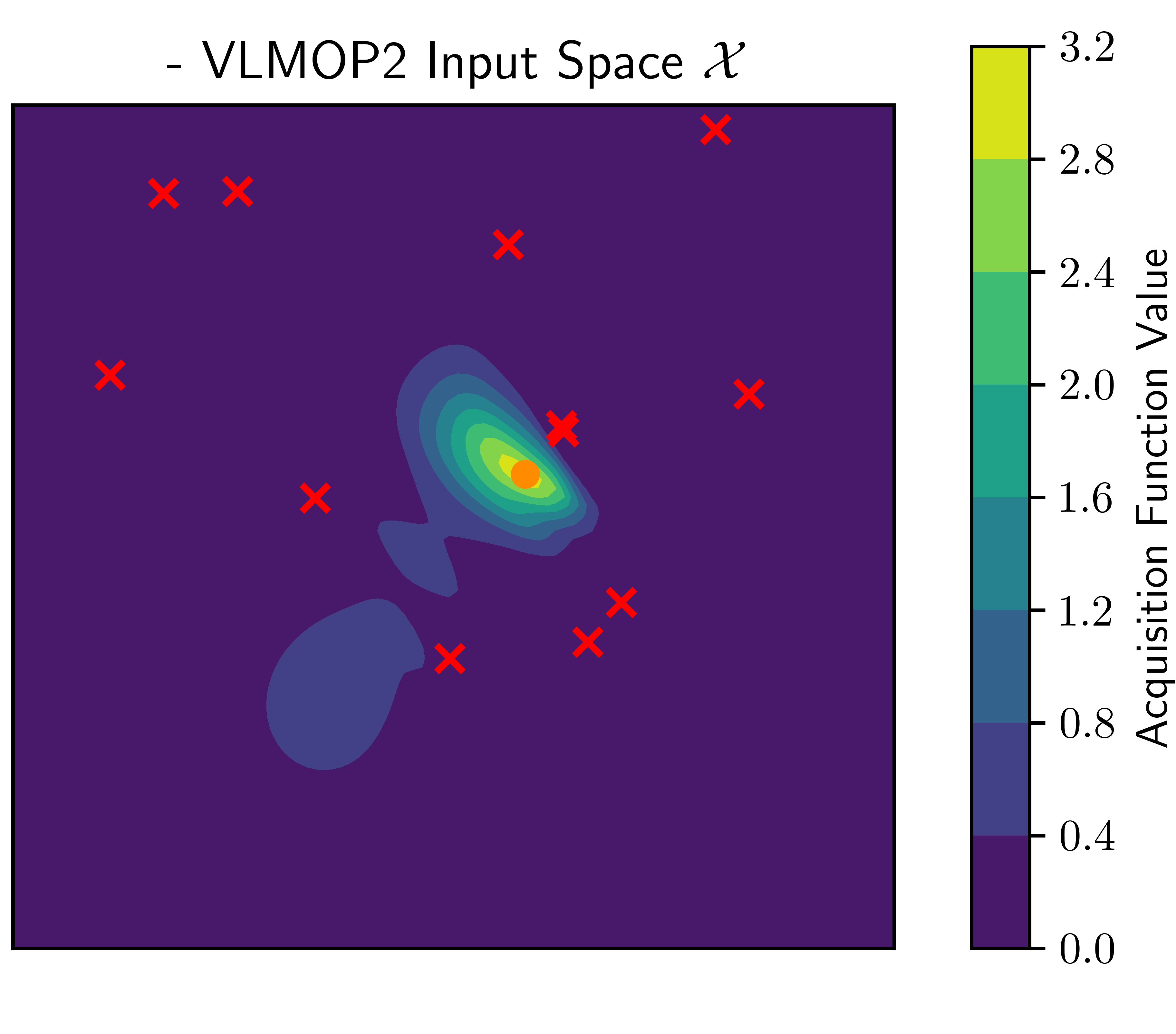
(c)

Figure 6: The $\varepsilon$ approach for mitigating clustering issues. a) The non-dominated region is extracted from the partitioning $\mathcal{P}$ based on the shifted Pareto frontier $\tilde{\mathcal{F}}_{\varepsilon}$. b) Relative to Fig. 5, the conservative estimation of $\tilde{A}$ has encouraged more exploration, i.e., candidate ($\bm{\sigma}_{\bm{x}}=[0.053400,0.032628]$). c) The corresponding exploration around the Pareto set in the input space.

Finally, this significant performance improvement is validated by the sensitivity analysis of $\varepsilon$ in Fig. 10, where the performance of the original approach $\tilde{\alpha}_{\{\text{PF}\}^{2}\text{ES}}(\tilde{A}(\tilde{\mathcal{F}}))$ is denoted as $\varepsilon=0$.

Appendix C PARALLEL VERSION q-{PF}²ES

C.1 Derivation of q-{PF}²ES

Consider the random variable $\bm{h}_{\bm{X}}=\{\bm{h}_{\bm{x}_{1}},...,\bm{h}_{\bm{x}_{q}}\}$, i.e., the objective-constraint observations that could arise from a parallel evaluation of a batch of $q$ points. In this scenario, we want to allocate a batch of $q$ points X that provide the most mutual information about the (feasible) Pareto frontier. With Eq. 4, we have:

$$I(\mathcal{F};\bm{h}_{\bm{X}})\geq\mathbb{E}_{\mathcal{F}}\left[\int_{\bm{h}_{\bm{x}}}p(\bm{h}_{\bm{X}}|\mathcal{F})\text{log}\frac{q(\bm{h}_{\bm{X}}|\mathcal{F})}{p(\bm{h}_{\bm{X}})}d\bm{h}_{\bm{X}}\right]$$ (16)

Given the Pareto frontier $\mathcal{F}$, we set the variational approximation of the ground-truth conditional distribution $p(\bm{h}_{\bm{X}}|\mathcal{F})$ as:

$$q(\bm{h}_{\bm{X}}|\mathcal{F})=\left\{\begin{aligned} &\frac{p(\bm{h}_{\bm{X}})}{Z_{{\overline{A}_{q}}}}\quad\bm{h}_{\bm{X}}\in\overline{A}_{q}\\ &0\quad\quad\quad\ \text{otherwise,}\\ \end{aligned}\right.$$ (17)

where $A_{q}\cup\overline{A}_{q}=\mathbb{R}^{q(M+C)}$, $A_{q}\in\mathbb{R}^{q(M+C)}$ is the union of the non-dominated feasible regions: $\{\bm{h}_{\bm{X}}\in\mathbb{R}^{q(M+C)}|\exists i\in\{1,...,q\},\bm{h}_{{\bm{x}}_{i}}\in A\}$ and $\overline{A}_{q}\in\mathbb{R}^{q(M+C)}$ is its complement $\{\bm{h}_{\bm{X}}\in\mathbb{R}^{q(M+C)}|\forall i\in\{1,...,q\},\bm{h}_{{\bm{x}}_{i}}\in\overline{A}\}$. An intuitive illustration of $A_{q}$ and $q(\bm{h}_{\bm{X}}|\mathcal{F})$ is provided in Fig. 7. Note, the practical interpretation of the conditional probability Eq. 17 is that, given $\mathcal{F}$, the outcome of the objective-constraint observation is expected to have zero probability of being in the feasible non-dominated region $A$ for any candidate point within the batch, as otherwise $\mathcal{F}$ is not a valid Pareto frontier.

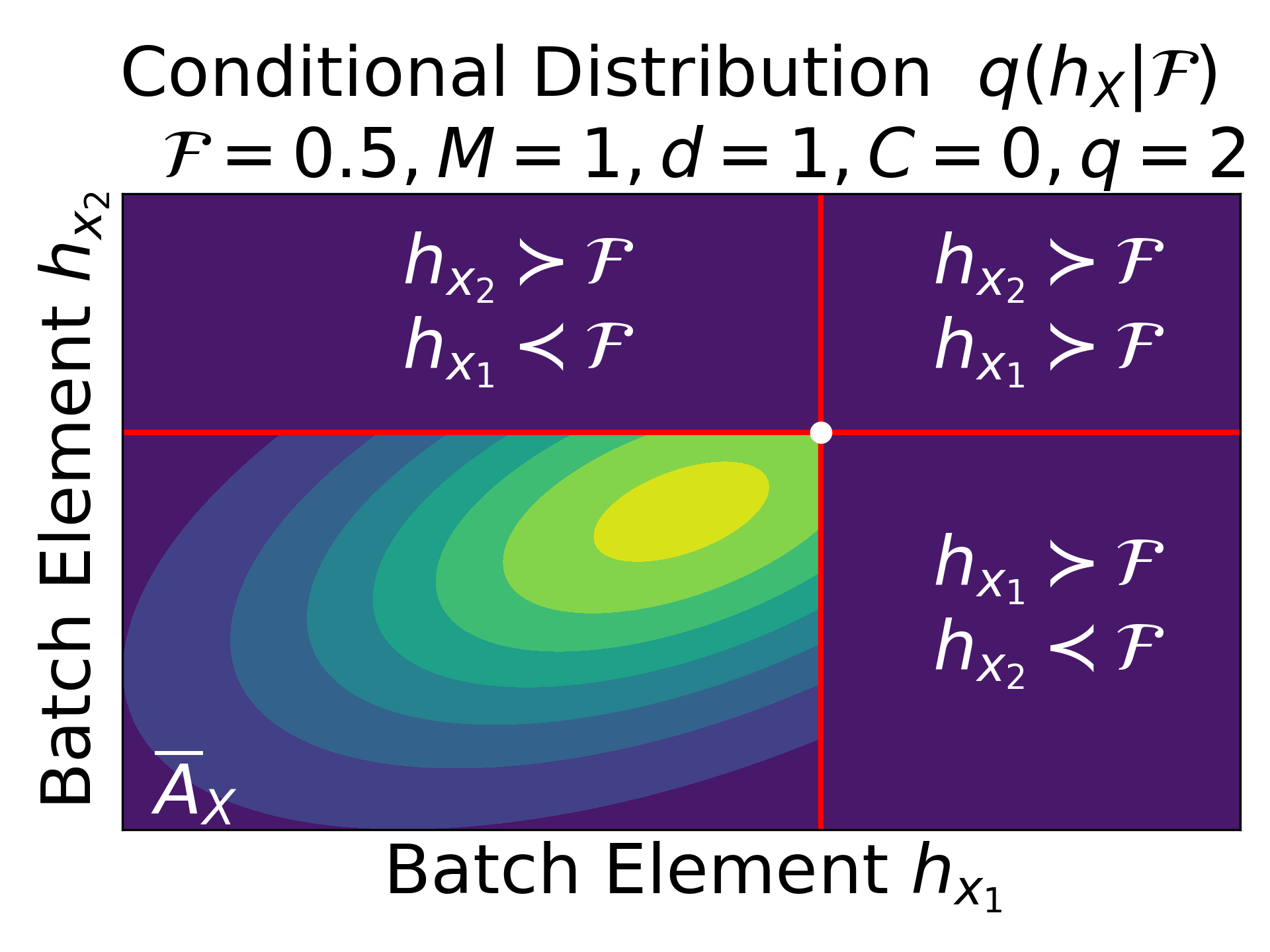
Figure 7: The batch conditional probability density $q(\bm{h}_{\bm{X}}|\mathcal{F})$ for $M=1$, $q=2$ and $C=0$. The problem degenerates to a batch single-objective optimization problem, where $\mathcal{F}$ collapses to a scalar value (the maximum) and the dominance operation is reduced to $>$. In this scenario, by conditioning on $\mathcal{F}$ (white dot), the objective space can be partitioned into 2 different subspaces: the union of the non-dominated feasible regions $A_{q}$ and its complement $\overline{A}_{q}$, see bottom-left plot. The condition of being in the region of $\overline{A}_{q}$ can be interpreted as: no point inside the batch is larger than $\mathcal{F}$. The concept can be generalized for arbitrary $M$, $q$ and $C$.

Following the same steps to motivate $\{\text{PF}\}^{2}$ES, we arrive at the following MC estimate of the resulting variational bound and the proposed batch extension of $\{\text{PF}\}^{2}$ES:

$$\alpha_{\text{q-}\{\text{PF}\}^{2}\text{ES}}\approx-\frac{1}{|\tilde{\mathbf{F}}|}\sum_{\tilde{\mathcal{F}}\in\tilde{\mathbf{F}}}\left[\text{log}\left(1-Z_{\tilde{A}_{q}(\tilde{\mathcal{F}}_{\bm{\varepsilon}})}\right)\right],$$ (18)

where $Z_{\tilde{A}_{q}}:=\int_{\tilde{A}_{q}}p(\bm{h}_{\bm{X}})d\bm{h}_{\bm{X}}$. i.e., the probability that there exists at least one batch element $\bm{h}_{\bm{x}_{l}}\in\bm{h}_{\bm{X}}$ such that $\bm{h}_{\bm{x}_{l}}\in\tilde{A}=\{\tilde{A}_{1},...,\tilde{A}_{N_{p}}\}$. We omit the notion $\tilde{\mathcal{F}}_{\bm{\varepsilon}}$ here as well as in Eq. 19,12 for notational simplicity.

To demonstrate the calculation of $Z_{\tilde{A}_{q}}$, it is convenient to utilize the notion of events. Define $\omega(\tilde{A},h_{\bm{X}})$ representing the event that there exists at least one batch element $\bm{h}_{\bm{x}_{l}}\in\bm{h}_{\bm{X}}$ such that $\bm{h}_{\bm{x}_{l}}\in\tilde{A}$ , it can be seen that $Z_{\tilde{A}_{q}}=p(\omega(\tilde{A},h_{\bm{X}}))$. Now, since $\tilde{A}=\{\tilde{A}_{1},...,\tilde{A}_{N_{p}}\}$, we know that $\omega(\tilde{A},h_{\bm{X}})=\bigcup_{i=1}^{N_{p}}\omega(\tilde{A}_{i},h_{\bm{X}})$, where $\omega(\tilde{A}_{i},h_{\bm{X}})$ represents there exists at least one batch element $\bm{h}_{\bm{x}_{l}}\in\bm{h}_{\bm{X}}$ such that $\bm{h}_{\bm{x}_{l}}\in\tilde{A}_{i}$. It can be also seen that $\omega(\tilde{A}_{i},h_{\bm{X}})=\bigcup_{l=1}^{q}\omega(\tilde{A}_{i},h_{{\bm{x}_{l}}})$ where $\omega(\tilde{A}_{i},h_{{\bm{x}_{l}}})$ is the $l$th batch element $h_{{\bm{x}_{l}}}$ is in $\tilde{A}_{i}$. Combine the two unions, and the fact that $\omega(\tilde{A}_{i},h_{{\bm{x}_{l}}})=\prod_{k=1}^{M+C}\left(\mathbbm{1}(A_{i_{l}}^{k}\leq\bm{h}_{\bm{x}_{l_{j}}}^{k}\leq A_{i_{u}}^{k})\right)$ representing $\bm{h}_{\bm{x}_{l}}$ is within the decomposed hypercube $\tilde{A}_{i}$, the event of $\omega(\tilde{A},h_{\bm{X}})$ can be written as:

$$\omega(\tilde{A},h_{\bm{X}})=\bigcup_{i=1}^{N_{p}}\left(\bigcup_{l=1}^{q}\omega(\tilde{A}_{i},h_{{\bm{x}_{l}}})\right)=\bigcup_{i=1}^{N_{p}}\left(\bigcup_{l=1}^{q}\left(\prod_{k=1}^{M+C}\left(\mathbbm{1}(\tilde{A}_{i_{l}}^{k}\leq\bm{h}_{\bm{x}_{l_{j}}}^{k}\leq\tilde{A}_{i_{u}}^{k})\right)\right)\right)$$ (19)

Finally, we are able to MC approximate the probability of this event:

$$Z_{\tilde{A}_{q}} =p\left(\omega(\tilde{A},\bm{h_{X}})\right)$$ (20)

$$\approx\frac{1}{N_{MC}}\sum_{j=1}^{N_{MC}}\left(\bigcup_{i=1}^{N_{p}}\left(\bigcup_{l=1}^{q}\left(\prod_{k=1}^{M+C}\left(\mathbbm{1}(\tilde{A}_{i_{l}}^{k}\leq\bm{h}_{\bm{x}_{l_{j}}}^{k}\leq\tilde{A}_{i_{u}}^{k})\right)\right)\right)\right)$$

$$\approx\frac{1}{N_{MC}}\sum_{j=1}^{N_{MC}}\left(max_{i}\left(max_{l}\left(\prod_{k=1}^{M+C}\left(\sigma\left(\frac{\bm{h}_{\bm{x}_{l_{j}}}^{k}-\tilde{A}_{i_{l}}^{k}}{\tau}\right)\cdot\sigma\left(\frac{\tilde{A}_{i_{u}}^{k}-\bm{h}_{\bm{x}_{l_{j}}}^{k}}{\tau}\right)\right)\right)\right)\right),$$

Note that the additional approximation introduced in Eq. 20 is caused by the relaxation of the categorical event (imposed by the indicator function) to a continuous approximation: $\mathbbm{1}(\tilde{A}_{i_{l}}^{k}\leq\bm{h}_{\bm{x}_{l_{j}}}^{k}\leq\tilde{A}_{i_{u}}^{k})\approx\sigma\left(\frac{\bm{h}_{\bm{x}_{l_{j}}}^{k}-\tilde{A}_{i_{l}}^{k}}{\tau}\right)\cdot\sigma\left(\frac{\tilde{A}_{i_{u}}^{k}-\bm{h}_{\bm{x}_{l_{j}}}^{k}}{\tau}\right)$. This makes the MC approximation suitable for gradient-based optimizers.

C.2 Monte Carlo Approximation of q-{PF}²ES and its Demonstration

We elaborate on how the MC approximation has been implemented here. Letting $\mathcal{\ell}:\mathbb{R}^{q(M+C)}\times A\rightarrow\mathbb{R}$ represents the utility function that calculate $Z_{\tilde{A}_{q}}$ as in Eq. 12, we can write the MC approximated q-{PF}²ES in terms of $\mathcal{\ell}$ as:

$$\alpha_{\text{q-}\{\text{PF}\}^{2}\text{ES}}\approx\tilde{\alpha}_{\text{q-}\{\text{PF}\}^{2}\text{ES}}=-\frac{1}{|\tilde{\mathbf{F}}|}\sum_{\tilde{\mathcal{F}}\in\tilde{\mathbf{F}}}\left[\text{log}\left(1-\frac{1}{N_{MC}}\sum_{j=1}^{N_{MC}}\mathcal{\ell}({\bm{h_{X}}}_{j},\tilde{A}_{q}(\tilde{\mathcal{F}}_{\bm{\varepsilon}}))\right)\right],$$ (21)

where $\tilde{\alpha}_{\text{q-}\{\text{PF}\}^{2}\text{ES}}$ represents the MC approximated acquisition function, we note $\tilde{A}_{q}(\tilde{\mathcal{F}}_{\bm{\varepsilon}})$ is independent of $\bm{X}$. With the aim of a consistent MC acquisition function gradient, we leverage the reparameterization trick (Kingma and Welling,, 2013) to generate samples of $\bm{h_{X}}$: since $\bm{h_{X}}\sim\mathcal{N}(\bm{m_{X}},L_{\bm{X}}L_{\bm{X}}^{T})$ where $\bm{m_{X}}\in\mathbb{R}^{q(M+C)}$, Cholesky factor $L_{\bm{X}}\in\mathbb{R}^{q(M+C)\times q(M+C)}$ , it can be generated via ${\bm{h_{X}}}=\bm{m_{X}}+L_{\bm{X}}\lambda$, where $\lambda\sim\mathcal{N}(\bm{0},\bm{I})$ and the base sample sets: $\{\lambda_{j}\}_{j=1}^{N_{MC}},\lambda_{j}\in\mathbb{R}^{q(M+C)}$ is holding through the whole process of acquisition function maximization, the largely preserved consistency can be shown via the chain rule of derivative as $\nabla_{\bm{X}}\tilde{\alpha}_{\text{q-}\{\text{PF}\}^{2}\text{ES}}=-\frac{1}{|\tilde{\mathbf{F}}|}\sum_{\tilde{\mathcal{F}}\in\tilde{\mathbf{F}}}\left[\frac{-\frac{1}{N_{MC}}\sum_{j=1}^{N_{MC}}\nabla_{\bm{X}}\mathcal{\ell}({\bm{h_{X}}}_{j},\tilde{A}_{q}(\tilde{\mathcal{F}}_{\bm{\varepsilon}}))}{\left(1-\frac{1}{N_{MC}}\sum_{j=1}^{N_{MC}}\mathcal{\ell}({\bm{h_{X}}}_{j},\tilde{A}_{q}(\tilde{\mathcal{F}}_{\bm{\varepsilon}}))\right)}\right]$, where each element within the $max$ function $\left(\prod_{k=1}^{M+C}\left(\sigma\left(\frac{\bm{h}_{\bm{x}_{l_{j}}}^{k}-\tilde{A}_{i_{l}}^{k}}{\tau}\right)\cdot\sigma\left(\frac{\tilde{A}_{i_{u}}^{k}-\bm{h}_{\bm{x}_{l_{j}}}^{k}}{\tau}\right)\right)\right)$ is differentiable. We use quasi-Monte Carlos to generate the base samples and refer Balandat et al., (2020); Daulton et al., (2020) for details of such an approximation.

As a proof of concept, we illustrate the effectiveness of q-{PF}²ES (with batch size $q=2$, and qMC sample size 128) on a one-dimensional Sinlinear-Forrester function (Table 3 of Qing et al., 2022a ). The progress plot of batch queries is provided in Fig. 8. It can be seen that the out-of-sample strategy is able to accurately recommend a Pareto frontier without false positives after five batches BO iterations.

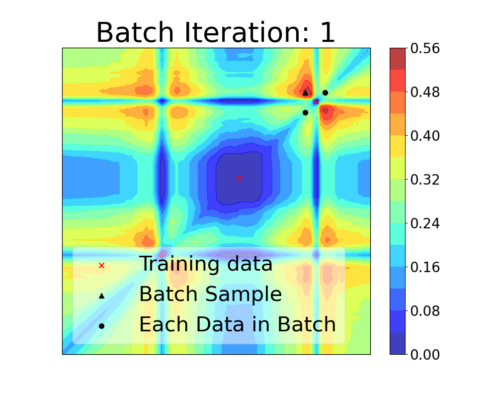
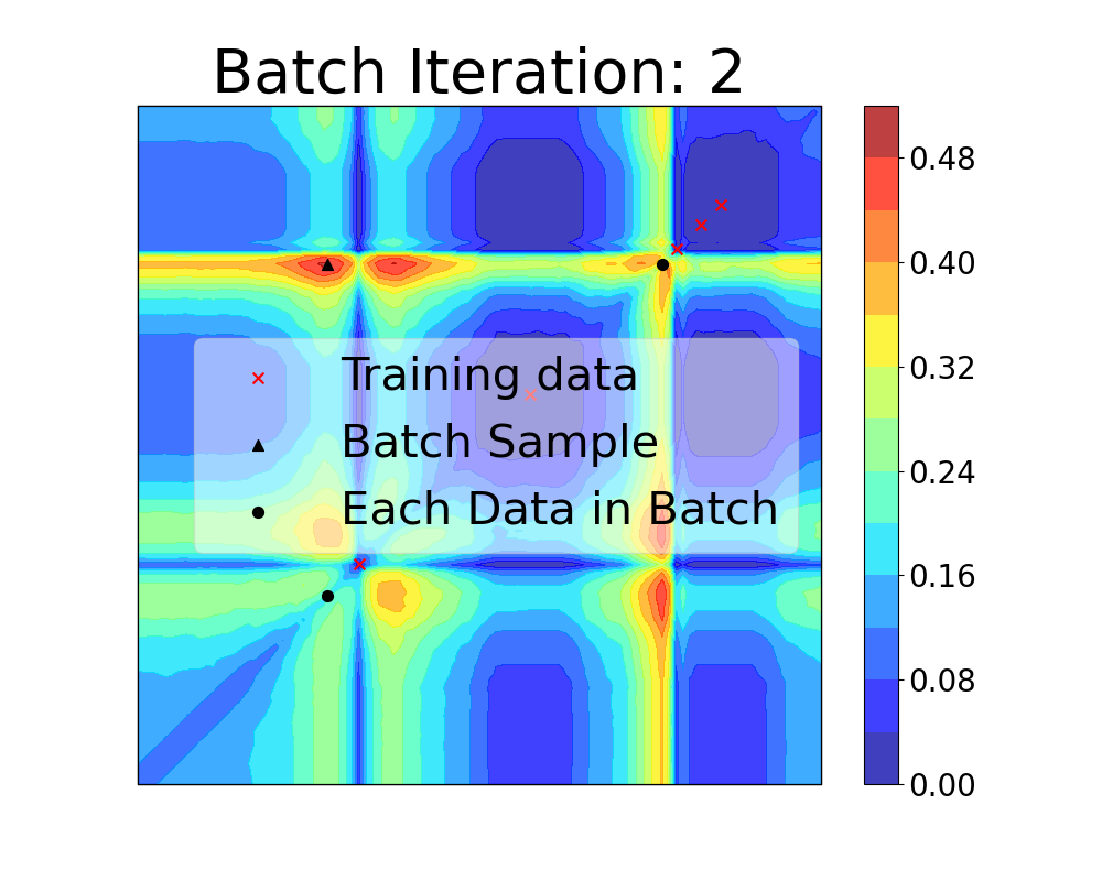
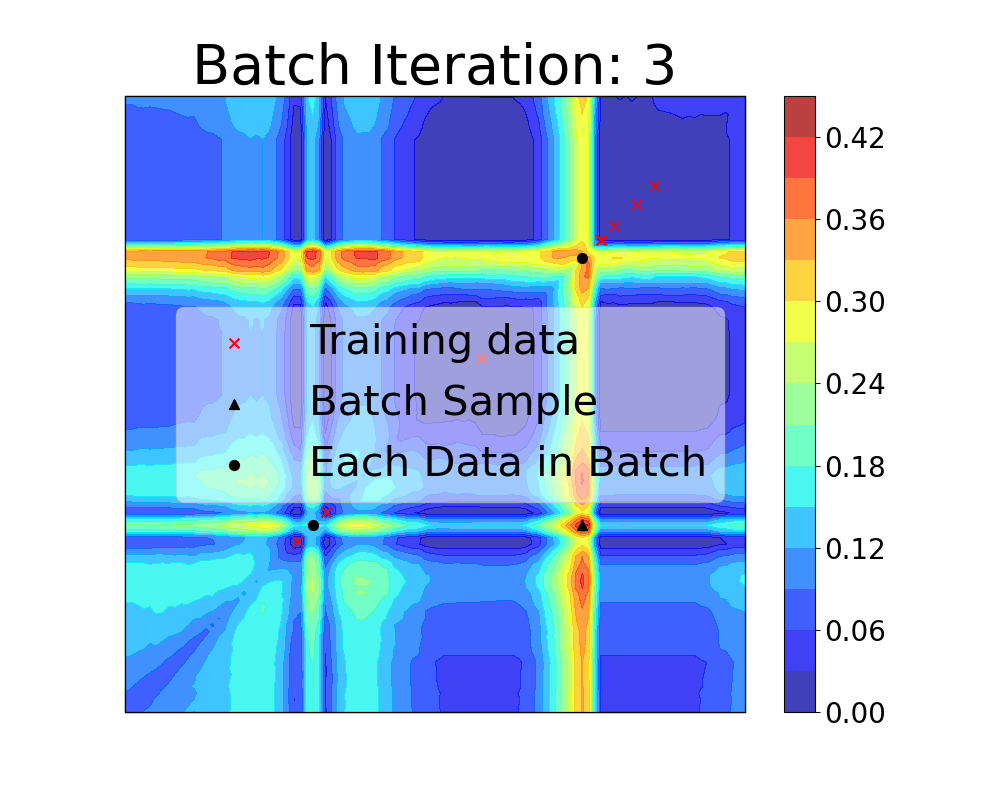
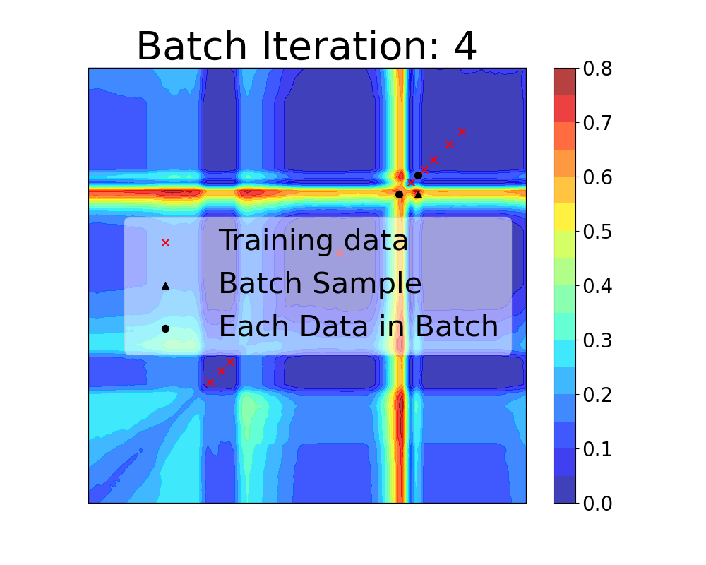
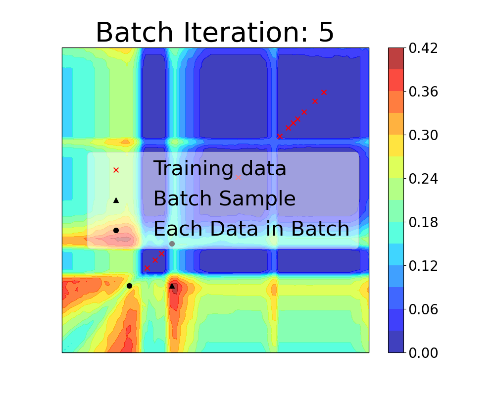
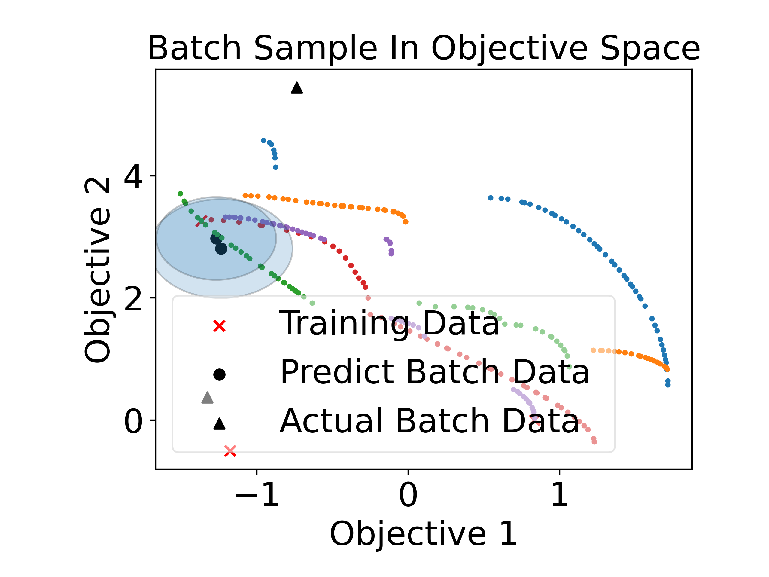
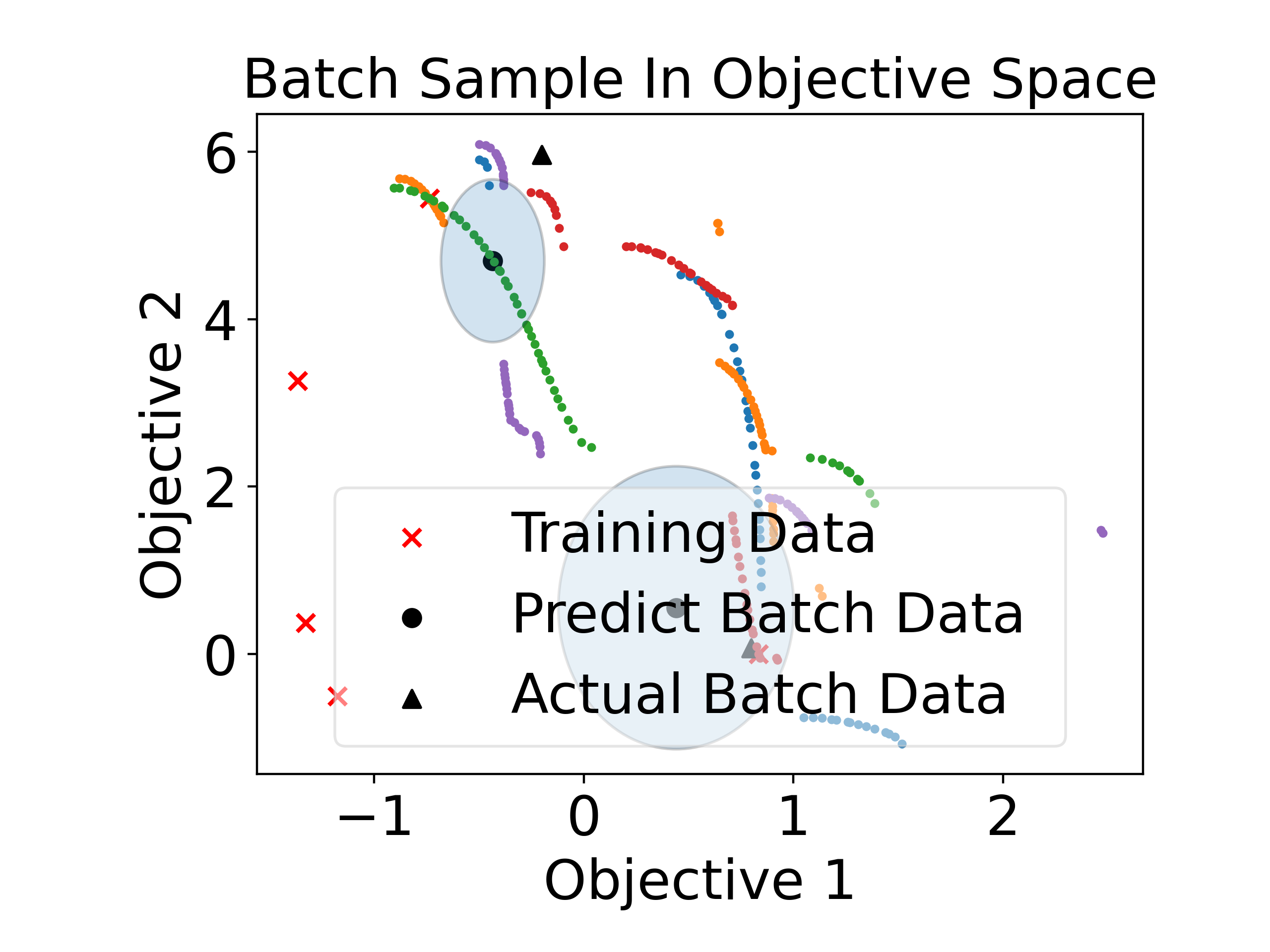
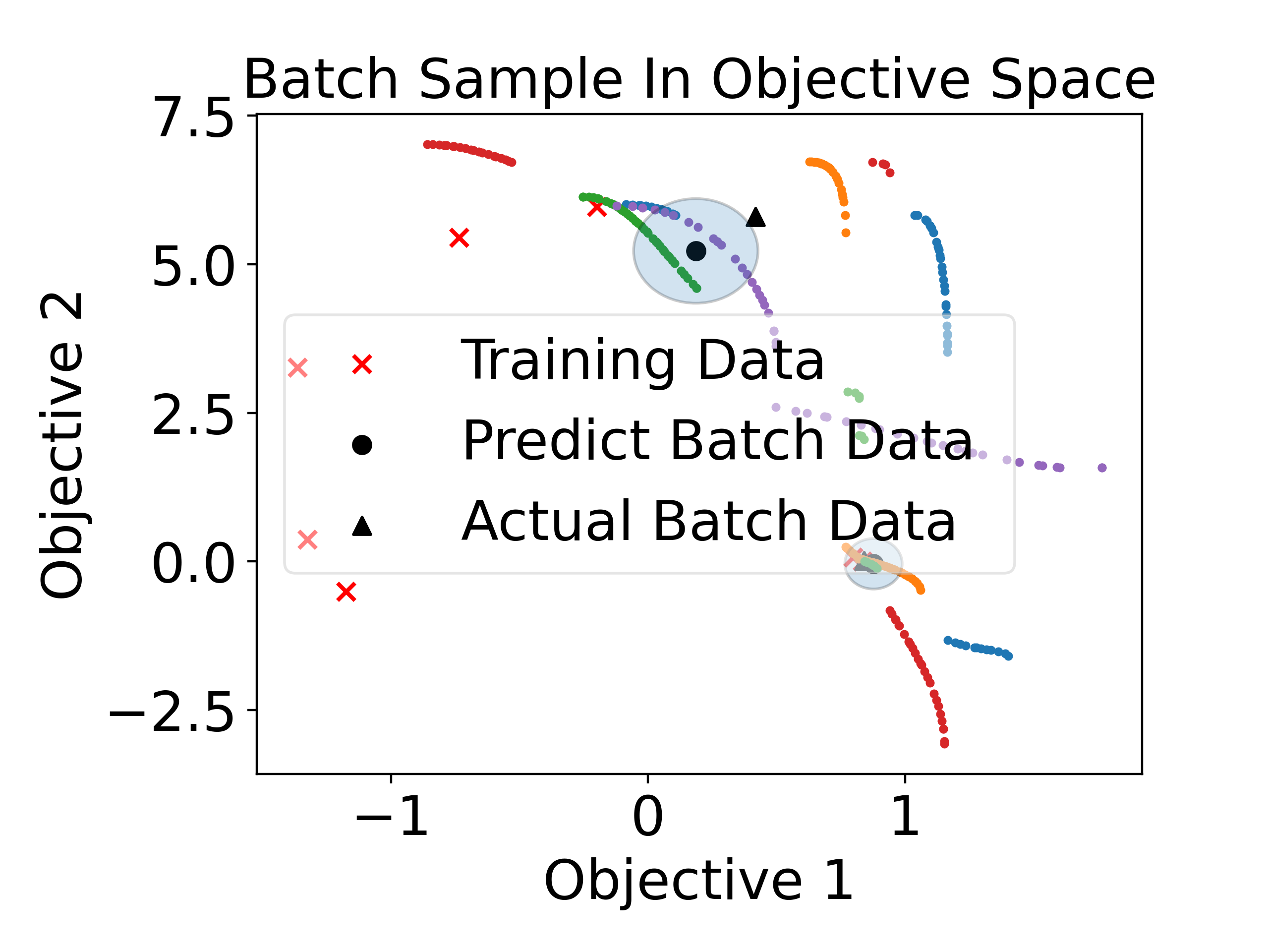
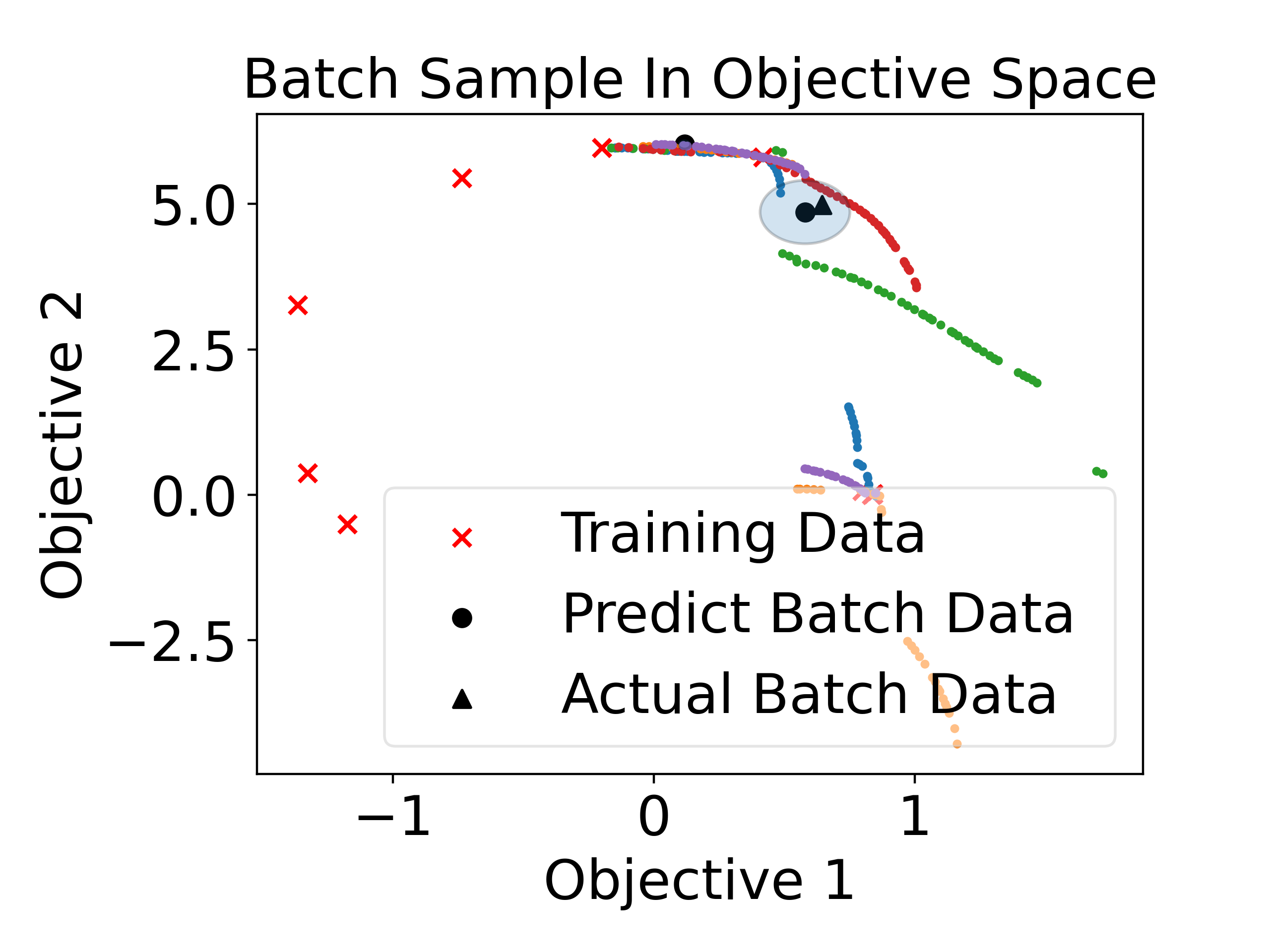
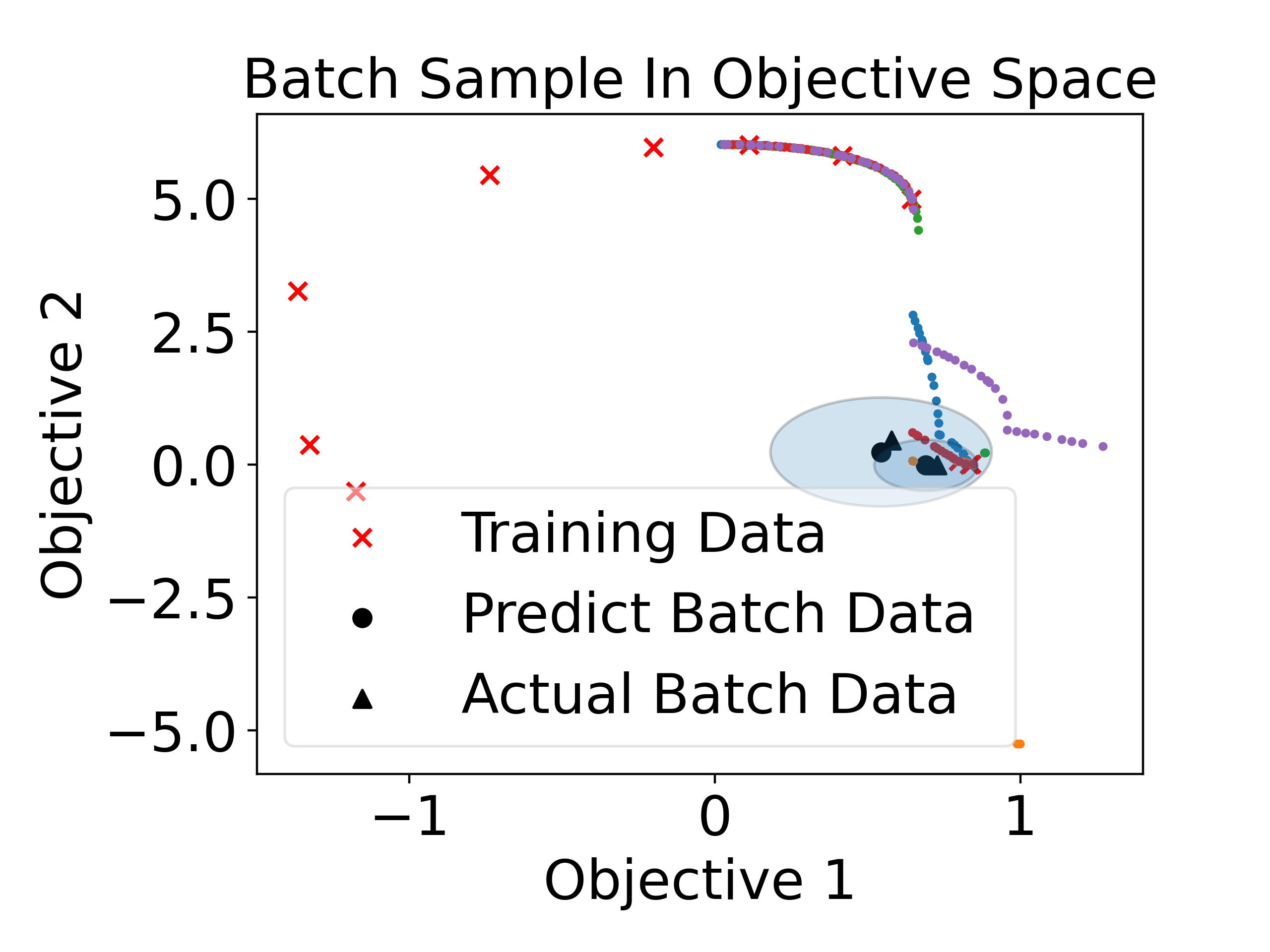
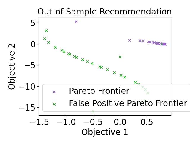
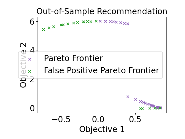
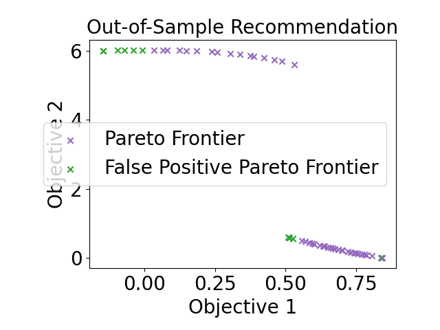
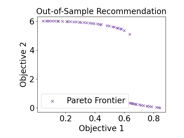
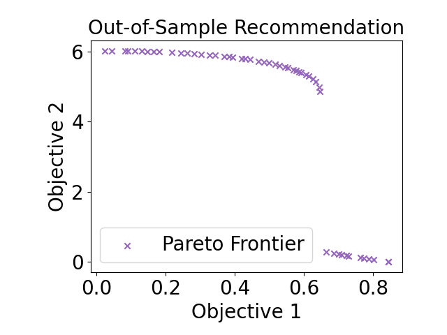
Figure 8: q-{PF}²ES on the inverted Sinlinear-Forrester problem ($d=1,M=2,C=0$), i.e., for maximization we take the negative of the objective functions, with $q=2$ starting from three training data points. The first row is contour of q-{PF}²ES in the concatenated batch input space. The second row represents the sampled Pareto frontiers $\bm{\tilde{F}}$ and the queried batches in the objective space (the shaded oval area is the $2\bm{\sigma}$ of the GP uncertainty). The third row shows the out-of-sample recommended Pareto frontiers after the batch query, with false positives denoted in green.

Appendix D ALTERNATIVE STRATEGY FOR SETTING $\varepsilon$

In the case of common bi-objective optimization ($M=2$) scenarios, $\varepsilon$ can also be specified using an alternative strategy. The motivation for this approach is that, under mild additional assumptions, $\varepsilon$ is closer to the infimum of the mutual information lower bound set (i.e., an ordered set of $\varepsilon$ with the lower bound property of the mutual information).

Proposition 1.

For a continuous Pareto Frontier $\mathcal{F}$ with $M=2$, given its finite approximation $\tilde{\mathcal{F}}$:= $\{\bm{f}^{*}|\bm{f}^{*}\in\mathcal{F}\}$ that satisfy $\forall k\in M$: $\exists\bm{f}^{*}\in\tilde{\mathcal{F}}s.t.\bm{f}_{k}^{*}=\underset{\bm{x}\in\mathcal{X}}{max}(\bm{f}_{k}(\bm{x}))$ and $|\tilde{\mathcal{F}}|\geq 2$, define its corresponding set for $k$th output $\tilde{\mathcal{F}^{k}}_{ord}$ ordered with $\leq$. Define $\bm{\varepsilon_{t}}:=[\varepsilon_{1},...,\varepsilon_{M}]$, where $\forall k\in M,\varepsilon_{k}=\underset{1\leq i\leq|\tilde{\mathcal{F}}|-1}{max}(\tilde{\mathcal{F}^{k}}_{{ord}_{i+1}}-\tilde{\mathcal{F}^{k}}_{{ord}_{i}})$. $\forall\bm{\varepsilon}\geq\bm{\varepsilon_{t}}$, with the hypervolume partition $\mathcal{P}(\tilde{\mathcal{F}_{\bm{\varepsilon}}})$ based on $\tilde{\mathcal{F}_{\bm{\varepsilon}}}:=\{\bm{f}+\bm{\varepsilon}|\bm{f}\in\tilde{\mathcal{F}}\}$, $I(\mathcal{F};\bm{h}_{\bm{x}})\geq\underset{|\tilde{\mathbf{F}}|\rightarrow\infty}{\textup{lim}}\tilde{\alpha}_{\{\text{PF}\}^{2}\text{ES}}(\tilde{A}(\tilde{\mathcal{F}}_{\bm{\varepsilon}}))$.

Proposition 1 states that under the extrema assumption (i.e., the discrete Pareto frontier preserves all extrema points in $\mathcal{F}$), specifying $\varepsilon$ as the maximum inner spacing between Pareto points within $\tilde{\mathcal{F}}$ per output dimension. One can subsequently define the non-dominated region $\tilde{A}$ based on the shifted Pareto frontier $\tilde{\mathcal{F}_{\bm{\varepsilon}}}$, which guarantees the acquisition function to be a lower bound of mutual information estimation (Eq. 8) when the Pareto frontier samples $|\tilde{\mathbf{F}}|\rightarrow\infty$. Here we elaborate on the proof of Proposition 1. We start with assuming an unconstrained multi-objective optimization problem. Note that the following proof also utilizes the well-established definition of strict and weak dominance (i.e., $\succ$ and $\succeq$ respectively) and the property of transitivity of dominance (i.e., $a\succeq b\succeq c\Rightarrow a\succeq c$), for which we refer to standard multi-objective optimization textbooks, e.g., Emmerich and Deutz, (2018).

Lemma 1.

For any discrete Pareto frontier $\tilde{\mathcal{F}^{*}}$ when $M=2$, with $\bm{\varepsilon}_{t}$ defined as in proposition 1, $\forall\bm{f}\in\tilde{A}(\tilde{\mathcal{F}^{*}})\cap\{\bm{f}|\forall k\in M:\bm{f}_{k}\leq max(\tilde{\mathcal{F}_{k}^{*}})\}$ , $\exists\bm{f}^{*}\in\tilde{\mathcal{F}^{*}}$ s.t. $\bm{f}^{*}\preceq\bm{f}+\bm{\varepsilon}_{t}$ and $\bm{f}^{*}$ is not unique.

Proof.

For any $k$th output, given that $\bm{f}_{k}\leq max(\tilde{\mathcal{F}_{k}^{*}})$, we know that $\exists k_{i}\in[1,|\tilde{\mathcal{F}}|-1]$: $\tilde{\mathcal{F}}^{k}_{{ord}_{k_{i}}}\leq\bm{f}_{k}\leq\tilde{\mathcal{F}^{k}}_{{ord}_{k_{i+1}}}$. $1^{\circ}$: if for $l\neq k$, $\tilde{\mathcal{F}}^{l}_{{ord}_{l_{|\tilde{F}|-i}}}\leq\bm{f}_{l}\leq\tilde{\mathcal{F}^{l}}_{{ord}_{l_{|\tilde{F}|-i+1}}}$, then we know that $\bm{f}_{k}+\varepsilon_{k}\geq\tilde{\mathcal{F}^{k}}_{{ord}_{k_{i+1}}}$ and $\bm{f}_{l}+\varepsilon_{l}\geq\tilde{\mathcal{F}^{l}}_{{ord}_{l_{|\tilde{F}|-i+1}}}$, hence $\bm{f}+\bm{\varepsilon}\succeq(\tilde{\mathcal{F}^{k}}_{{ord}_{k_{i+1}}},\tilde{\mathcal{F}^{l}}_{{ord}_{l_{|\tilde{F}|-i+1}}})$. Since $(\tilde{\mathcal{F}^{k}}_{{ord}_{k_{i+1}}},\tilde{\mathcal{F}^{l}}_{{ord}_{l_{|\tilde{F}|-i+1}}})\succeq(\tilde{\mathcal{F}^{k}}_{{ord}_{k_{i}}},\tilde{\mathcal{F}^{l}}_{{ord}_{l_{|\tilde{F}|-i+1}}})$ and $(\tilde{\mathcal{F}^{k}}_{{ord}_{k_{i+1}}},\tilde{\mathcal{F}^{l}}_{{ord}_{l_{|\tilde{F}|-i+1}}})\succeq(\tilde{\mathcal{F}^{k}}_{{ord}_{k_{i+1}}},\tilde{\mathcal{F}^{l}}_{{ord}_{l_{|\tilde{F}|-i}}})$, the lemma holds; $2^{\circ}$: if for $l\neq k$, $\bm{f}_{l}>\tilde{\mathcal{F}^{l}}_{{ord}_{l_{|\tilde{F}|-i+1}}}$. Finally it can be shown that $(\tilde{\mathcal{F}^{k}}_{{ord}_{k_{i+1}}},\tilde{\mathcal{F}^{l}}_{{ord}_{l_{|\tilde{F}|-i+1}}})\succeq(\tilde{\mathcal{F}^{k}}_{{ord}_{k_{i}}},\tilde{\mathcal{F}^{l}}_{{ord}_{l_{|\tilde{F}|-i+1}}})$ and $(\tilde{\mathcal{F}^{k}}_{{ord}_{k_{i+1}}},\tilde{\mathcal{F}^{l}}_{{ord}_{l_{|\tilde{F}|-i+1}}})\succeq(\tilde{\mathcal{F}^{k}}_{{ord}_{k_{i+1}}},\tilde{\mathcal{F}^{l}}_{{ord}_{l_{|\tilde{F}|-i}}})$. ∎

Lemma 2.

For a given discrete Pareto frontier $\tilde{\mathcal{F}}$ with $\bm{\varepsilon}_{t}$ as defined in proposition 1, $\tilde{A}(\tilde{\mathcal{F}_{{\varepsilon}_{t}}})\subseteq A(\mathcal{F})$.

Proof.

Note the necessary condition for $\tilde{A}(\tilde{\mathcal{F}}_{\bm{\varepsilon}_{t}})\subseteq A(\mathcal{F})$ is $\forall\bm{f}\in\tilde{A}(\tilde{\mathcal{F}}_{\bm{\varepsilon}_{t}})$: $\bm{f}\in A(\mathcal{F})$. Proof by contradiction: suppose $\exists\bm{f}\in\tilde{A}(\tilde{\mathcal{F}}_{\bm{\varepsilon}_{t}})$ s.t. $\bm{f}\notin A(\mathcal{F})$, hence $\bm{f}\in\overline{A}(\mathcal{F})$. This implies $\exists\bm{f}^{\prime}\in\mathcal{F}:\bm{f}^{\prime}\succeq\bm{f}\Rightarrow\bm{f}^{\prime}+\bm{\varepsilon}_{t}\succeq\bm{f}+\bm{\varepsilon}_{t}$. $1^{\circ}$: Suppose $\forall k\in M$: $\bm{f}_{k}\leq max(\tilde{\mathcal{F}}_{{\bm{\varepsilon}_{t}}_{k}})$, with lemma 1, by setting $\tilde{\mathcal{F}^{*}}=\tilde{\mathcal{F}}_{\bm{\varepsilon}_{t}}$ we know $\exists\bm{f}^{\prime\prime}\in\tilde{\mathcal{F}}_{\bm{\varepsilon}_{t}}$ s.t. $\bm{f}^{\prime\prime}\preceq\bm{f}+\bm{\varepsilon}_{t}$, then $\bm{f}^{\prime}+\bm{\varepsilon}_{t}\succeq\bm{f}+\bm{\varepsilon}_{t}\succeq\bm{f}^{\prime\prime}\Rightarrow\bm{f}^{\prime}\succeq\bm{f}^{\prime\prime}-\bm{\varepsilon}_{t}$, since $\bm{f}^{\prime\prime}-\bm{\varepsilon}_{t}\in\mathcal{F}$, due to the definition of a Pareto frontier this can only be hold when $\bm{f}^{\prime\prime}-\bm{\varepsilon}_{t}=\bm{f}^{\prime}$, which contradicts with its non-unique property, hence lemma holds; $2^{\circ}$: Suppose $\exists k\in M\ s.t.\ \bm{f}_{k}>max(\tilde{\mathcal{F}}_{{\bm{\varepsilon}_{t}}_{k}})$, since according to the definition of $\tilde{\mathcal{F}}$, $max(\tilde{\mathcal{F}}_{{\bm{\varepsilon}_{t}}_{k}})=max(\mathcal{F}_{k})+{\bm{\varepsilon}_{t}}_{k}$, this results $\bm{f}_{k}>max(\mathcal{F}_{k})$ and hence $\bm{f}\in A(\mathcal{F})$, contradicting with $\bm{f}\in\overline{A}(\mathcal{F})$.

∎

Eventually, the proof of Proposition 1 becomes straightforward: with lemma 2 and Eq. 6 we have $I(\mathcal{F};\bm{h}_{\bm{x}})\geq-\mathbb{E}_{\mathcal{F}}\left[\text{log}\left(1-Z_{A(\mathcal{F})}\right)\right]=\underset{|\mathbf{F}|\rightarrow\infty}{\text{lim}}-\frac{1}{|\mathbf{F}|}\sum_{\mathcal{F}\in\mathbf{F}}\left[\text{log}\left(1-Z_{A(\mathcal{F})}\right)\right]\geq\underset{|\tilde{\mathbf{F}}|\rightarrow\infty}{\text{lim}}\tilde{\alpha}_{\{\text{PF}\}^{2}\text{ES}}(\tilde{A}(\tilde{\mathcal{F}}_{\bm{\varepsilon}}))$ since $Z_{A(\mathcal{F})}\geq Z_{\tilde{A}(\tilde{\mathcal{F}}_{\bm{\varepsilon}})}$.

Remark that the proposition 1 is also valid for CMOO when $\mathcal{F}\neq\phi$ (the extrema condition in CMOO needs to be generalized for constraints). In reality, $\mathcal{F}$ is not continuous for all problems, unfortunately. Clustering techniques (e.g., Schubert et al., (2017)) can be utilized as a pre-processing step to satisfy the condition of the proposition. Nevertheless, this does increase the complexity of the method. For $M>2$, proposition 1 does not hold since $\bm{\varepsilon}$, as defined using the maximum inner spacing, can not guarantee that $\tilde{A}(\tilde{\mathcal{F}_{\varepsilon}})\subseteq A(\mathcal{F})$, and the choice of $\bm{\varepsilon}$ can be correlated with the choice of partitioning strategy $\mathcal{P}$.

The practical implementation of the original acquisition function {PF}²ES-c, as well as using the proper $\bm{\varepsilon}$ approach based on proposition 1 ({PF}²ES-lb) is detailed in Algorithm 1 and 2, respectively. Note that lines 2-9 in both algorithms only need to be calculated once per BO iteration.

D.1 Comparing strategies for setting $\varepsilon$

We investigate the two different approaches for setting $\bm{\varepsilon}$ for two bi-objective optimization problems. Namely, VLMOP2 and C-BraninCurrin as provided in Table 1, both with continuous Pareto frontiers. The results are shown in Fig. 9 where we refer to the heuristical approach as {PF}²ES-4% (i.e.,$c=0.04$) and the approach above as {PF}²ES-lb. From the in-sample regret, it can be seen that {PF}²ES-lb can be more greedy than {PF}²ES-4%, although it is less competitive in terms of out-of-sample recommendations for C-BraninCurrin. As conclusion, both strategies lead to comparable performance. Hence, we propose to simply utilize the heuristic approach which does not depend on extra assumptions and generalizes better with respect to $M$.

Algorithm 1 Practical implementation of {PF}²ES-c

1:Input: a candidate $\bm{x}$; GP models for objectives (and constraints): $\mathcal{M}$, heuristic shifting percentage $c$.

2:for $i=1,...,|\mathcal{F}|$ do

3:     generate $i$th GP parametric trajectory approximations (see e.g., Eq. 3, 4 of Qing et al., 2022b ).

4:     Apply NSGA2 to GP trajectories to obtain Pareto frontier samples $\tilde{\mathcal{F}}$

5:     for $k=1,...,M$ do:

6:         $\epsilon_{k}=c\cdot\left(max(\tilde{\mathcal{F}^{k}})-min(\tilde{\mathcal{F}^{k}})\right)$

7:     end for

8:     $\tilde{\mathcal{F}}_{\varepsilon}=\tilde{\mathcal{F}}+\varepsilon$

9:     Partition $\tilde{A}:\tilde{A}=\mathcal{P}(\tilde{\mathcal{F}}_{\varepsilon})$

10:end for

11:Return {PF}²ES-c (Eq. 10).

Algorithm 2 Practical implementation of {PF}²ES-lb

1:Input: a candidate $\bm{x}$; GP models for objectives (and constraints): $\mathcal{M}$.

2:for $i=1,...,|\mathcal{F}|$ do

3:     generate $i$th GP parametric trajectory approximations (see, e.g., Eq. 3, 4 of Qing et al., 2022b ).

4:     Apply NSGA2 to GP trajectories to obtain Pareto frontier samples $\tilde{\mathcal{F}}$

5:     for $k=1,...,M$ do:

6:         $\varepsilon_{k}=\underset{1\leq i\leq|\tilde{\mathcal{F}}|-1}{max}(\tilde{\mathcal{F}^{k}}_{{ord}_{i+1}}-\tilde{\mathcal{F}^{k}}_{{ord}_{i}})$ as in proposition 1

7:     end for

8:     $\tilde{\mathcal{F}}_{\varepsilon}=\tilde{\mathcal{F}}+\bm{\varepsilon}$

9:     Partition $\tilde{A}:\tilde{A}=\mathcal{P}(\tilde{\mathcal{F}}_{\varepsilon})$

10:end for

11:Return {PF}²ES-lb (Eq. 10).

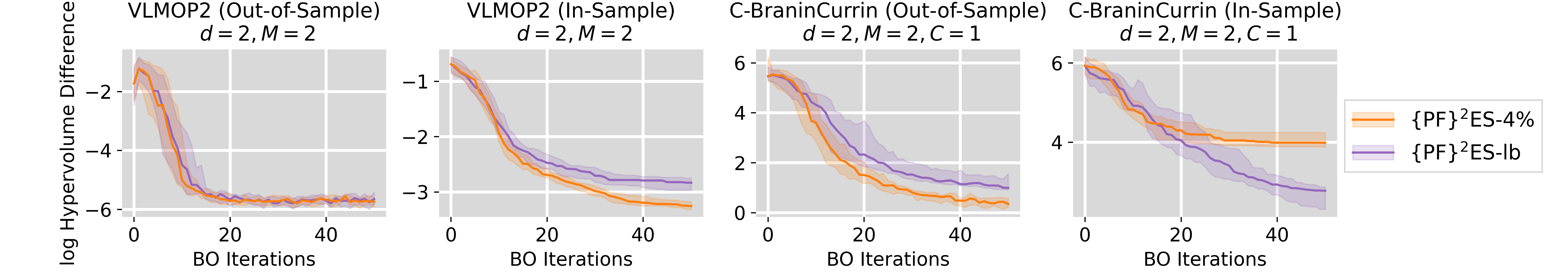
Figure 9: Comparing strategies for setting $\bm{\varepsilon}$ for two synthetic benchmark functions.

Appendix E EXPERIMENTAL DETAILS

E.1 Synthetic problems and setting the reference point

We benchmark on synthetic problems regularly used within the literature. Details are given in Table 1, together with the reference point used in the uncertainty calibration (i.e., Fig. 3) and for performance metric (i.e., Fig. 4, 5). Note that the ideal hypervolume utilized to calculate the log hypervolume difference performance metric is set optimistically to guarantee a well-behaved performance metric.

Table 1: Details of the synthetic problems and reference point settings

Problem	Formulation	$d$	$M$	$C$	Reference point	Reference point	Ideal
					(uncertainty	(regret)	Hypervolume
					calibration)		(regret)
VLMOP2	Table 1 of Van Veldhuizen and Lamont, (1999)	2	2	0	$[3,3]$	$[1.2,1.2]$	0.77157
BraninCurrin	Appendix E.2 of (Daulton et al.,, 2020)	2	2	0	$[2000,50]$	$[18.0,6.0]$	60.0000
ZDT1	Eq. 7 of Zitzler et al., (2000)	5	2	0	$[15,15]$	$[2.5,2.5]$	5.90453
ZDT2	Eq. 8 of Zitzler et al., (2000)	5	2	0	$[15,15]$	$[2.5,2.5]$	5.57236
Four Bar Truss	Eq. 21 of Dauert, (1993)	4	2	0	NA	$[3400,0.05]$	81.9590
DTLZ4 (App I.2)	Eq. 24 of Deb et al., (2005)	8	2	0	NA	$[2.5,2.5]$	$5.45327$
DTLZ4 (App I.3)	Eq. 24 of Deb et al., (2005)	5	3	0	NA	$[2.5,2.5,2.5]$	$15.0080$
C-BraninCurrin	Appendix E.2 of Daulton et al., (2020)	2	2	1	$[2000,100]$	$[80.0,12.0]$	606.752
Constr-EX	Eq. 7.2 of Deb and Kalyanmoy, (2001)	2	2	2	$[2,50]$	$[1.1,10.0]$	5.30186
SRN	Eq. 10 of Srinivas and Deb, (1994)	2	2	2	$[1500,500]$	$[250,50]$	46205.0
C2-DTLZ2	Section 4.6 of Deb, (2019)	4	2	1	$[10,250]$	$[2.5,2.5]$	5.43594
Disc Brake Design	Section 3.4 of Ray and Liew, (2002)	4	2	5	NA	$[8.0,4.0]$	17.6882
OSY (App I.2)	Sec 4.3 of Osyczka and Kundu, (1995)	6	2	6	NA	$[50,100]$	$25344.9$
Marine Design (App I.3)	CRE32 of Tanabe and Ishibuchi, (2020)	6	3	9	NA	$[-700,13000,3500]$	$6991669$

E.2 Out-of-sample recommendation strategy

For both MOO and CMOO problems, the feasible Pareto optimal inputs $\bm{X}_{r}$ is recommended using a conservative model-based approach similar to Garrido-Merchán and Hernández-Lobato, (2020); Ungredda and Branke, (2021). The recommendation task can be formulated as a MOO problem:

$$\underset{\bm{x}\in\mathcal{X}}{maximize}\ \bm{m}^{1},\bm{m}^{2},...,\bm{m}^{M}$$ (22)

$$s.t.,1-\Phi(\frac{\bm{m}^{M+1}-\eta^{1}}{\bm{\sigma}^{M+1}})\geq C_{Fea},...,1-\Phi(\frac{\bm{m}^{M+C}-\eta^{C}}{\bm{\sigma}^{M+C}})\geq C_{Fea}$$

where $m$ and $\sigma$ represent the GP poster mean and standard deviation, respectively. We expect all the recommendations to be feasible in our empirical experiments, hence $C_{Fea}$ is set to 0.95 and is decreased with 0.05 in case no feasible solution exists (i.e., $\bm{X}_{r}=\phi$), $\eta^{C}=0.5\%\cdot\left(max(\bm{H}^{C})-min(\bm{H}^{C})\right)$. In practice, we empirically find that while an aggressive recommendation strategy (e.g., $C_{Fea}=0.5,\eta=0$) can possibly contain infeasible candidates, the recommended candidates are able to cover the real Pareto frontier faster and the constraints are often only violated with a tiny amount (e.g., $1e-3$ level), which is tolerable for some applications. Hence, the practitioner is recommended to choose $C_{Fea}$ and $\eta$ according to the tolerance to constraint violations.

E.3 Setup details of different acquisition functions

We provide configuration details for different information-theoretic acquisition functions used in the comparison.

EHVI is using the Trieste (Berkeley et al.,, 2022) implementation. The dynamic reference point specification strategy (Knudde et al.,, 2017) is utilized:

$$r_{ref}=max(\tilde{\mathcal{F}})+2\cdot\frac{max(\tilde{\mathcal{F}})-min(\tilde{\mathcal{F}})}{|\tilde{\mathcal{F}}|}$$ (23)

qEHVI is based on the Trieste (Berkeley et al.,, 2022) implementation and extended with a random quasi-Monte Carlo (qMC) method for batch reparameterization sampling(see Eq. 15 of Daulton et al., (2020))). 128 qMC samples are used to approximate the hypervolume improvement.

The qEHVI paper does not provide a dynamic reference point strategy for CMOO. Denoting the outcome of objective function on training data as $\bm{F}$, the following strategy is used:

$$r_{ref}=\left\{\begin{array}[]{ll}max(\tilde{\mathcal{F}})+2\cdot\frac{max(\tilde{\mathcal{F}})-min(\tilde{\mathcal{F}})}{|\tilde{\mathcal{F}}|}&\tilde{\mathcal{F}}\neq\phi\\ max(\bm{F})+2\cdot\frac{max(\bm{F})-min(\bm{F})}{|\bm{F}|}&\tilde{\mathcal{F}}=\phi\\ \end{array}\right.$$ (24)

EHVI-PoF is a common strategy for handling CMOO. In case there are no predicted feasible observations on the training data, the probability of feasibility function will be used for locating a feasible observation first. For EHVI-PoF, the same reference point setting as EHVI is utilized, where $\tilde{\mathcal{F}}$ is the feasible Pareto frontier.

Information-theoretic acquisition functions For PESMO, MESMOC+ and PPESMOC, the implementations of the accompanying papers are used and implement the remaining acquisition functions ourselves. While we aim to use similar settings for all algorithms (e.g., the Pareto frontier number, the population sizes for NSGA2), the provided implementation of PESMO, MESMOC+, and PPESMOC still have different settings, see Table 2.

Table 2: Configurations of different information-theoretic acquisition functions.

	Pareto Frontier Sample Strategy	Pareto Frontier Samples	Out-of-sample Recommendation Strategy
{PF}2ES (for MOO)	NSGA2	5	NSGA2
PFES	NSGA2	5	NSGA2
MESMO	NSGA2	5	NSGA2
PESMO	Monte Carlo	1	NSGA2
q-{PF}2ES (for MOO)	NSGA2	5	NSGA2
{PF}2ES (for CMOO)	NSGA2*	5	NSGA2*
MESMOC	NSGA2*	5	NSGA2*
MESMOC+	Monte Carlo	1	Monte Carlo
q-{PF}2ES (for CMOO)	NSGA2*	5	NSGA2*
PPESMOC	Monte Carlo	1	Monte Carlo

Appendix F SENSITIVITY ANALYSIS OF THE HYPERPARAMETERS OF {PF}²ES AND q-{PF}²ES

F.1 Parameter $\varepsilon$

We conduct a sensitivity analysis for setting $\bm{\varepsilon}$ to determine its effect on the performance of the acquisition function. The results are depicted in Fig. 10, with results of both in-sample, and out-of-sample regret, as well as the uncertainty calibration of the Pareto frontier.

Figure 10: Sensitivity analysis of $\varepsilon$ on the performance of {PF}²ES.

It can be seen that $\bm{\varepsilon}$ is less sensitive in terms of out-of-sample regret within the range of $3\%-5\%$. A too-small value will not mitigate the clustering issue, while a large value of $\varepsilon$ can cause too much exploration resulting in a deterioration of the in-sample regret. Importantly, using $\bm{\varepsilon}$ is helpful for a faster reduction of the uncertainty of the Pareto frontier.

F.2 Number of Monte Carlo samples for q-{PF}²ES

We conduct an empirical sensitivity analysis of the MC sample size used in approximating the q-{PF}²ES (i.e., Eq. 12) and its effect on the performance. The results on two different benchmark functions are provided in Fig. 11. As expected, it can be seen that with an out-of-sample recommendation strategy, a larger MC sample size can positively affect the performance of the acquisition function. The benefit is more obvious for the in-sample recommendation strategy.

Figure 11: The performance difference of q-{PF}²ES with respect to different MC sample sizes.

Appendix G COMPUTATIONAL COMPLEXITY OF {PF}²ES AND q-{PF}² ES

For the information-theoretic acquisition function, generating the Pareto frontier approximation (i.e., line 3-9 of Algorithm 1,2) is treated separately as the initialization cost, while the cost of evaluating the acquisition functions is termed as evaluation cost.

Initialization cost The initialization of {PF}²ES consists of two parts: generation of $\tilde{\mathcal{F}}$ samples and calculate $\tilde{A}(\tilde{\mathcal{F}})$ by utilizing a hypervolume decomposition $\mathcal{P}$ on $\tilde{\mathcal{F}}$. The cost of the former, ignoring the non-dominated sorting complexity of NSGA2 which is $\mathcal{O}(M|\tilde{\mathcal{F}}|^{2})$ (Deb et al.,, 2002), breaks down to the cost of evaluating the GP spectral samples, which is linear with the number of random Feature features. The hypervolume decomposition strategy (Lacour et al.,, 2017) utilized in this research has a complexity of $\mathcal{O}(|\tilde{\mathcal{F}}|^{\lfloor\frac{M}{2}\rfloor+1})$. However, both {PF}²ES and q-{PF}²ES are agnostic to the choice of $\mathcal{P}$.

Evaluation cost

- {PF}²ES By denoting the maximum number of cells across the set of Pareto frontier samples $\tilde{\bm{F}}$ as $max(N_{p})$, the computational complexity of evaluate {PF}²ES is: $\mathcal{O}\left(max(N_{p})M\right)$ .

- q-{PF}²ES We omit the cost of the batch reparameterization sampling (which is $\mathcal{O}((M+C)q)$) and hence, the evaluation cost of q-{PF}²ES itself is: $\mathcal{O}\left(max(N_{p})qN_{MC}M\right)$.

Appendix H COMPARING RUNNING TIMES

The following experiments are conducted in parallel per batch of ten on a Linux server with 256 GB RAM. The results are depicted in Table 3. In general, the joint batch acquisition function q-{PF}²ES requires a longer time to query a batch of samples than {PF}²ES. Besides the additional computational complexity introduced by the MC approximation, cfr. Section G, this can be attributed to an increase in difficulty for the multi-start L-BFGS-B optimizer as illustrated in Fig. 12. We also note that, though the {PF}²ES-KB consumes similar time as other batch strategies, its computationally cost grows much faster w.r.t. $q$ as it requires additional sampling of the Pareto frontier $\tilde{\mathcal{F}}$. For PPESMOC, we generally observe a longer average query time than the original paper which reports the median (Table 1 of Garrido-Merchán and Hernández-Lobato, (2020)), and the query time grows drastically with the number of iterations (e.g., the batch query time for C2DTLZ2 grows from around 20 minutes per batch sample to almost 3 hours when approaching the maximum number of batch iterations).

Table 3: Wall time for optimizing the acquisition function in seconds on a CPU (2x Silver 4210 CPU @ 2.20GHz). The mean and 2 times the standard deviations are reported across 30 runs.

	VLMOP2	BraninCurrin	ZDT1	ZDT2
{PF}2ES	$47.38\pm 4.28$	$47.01\pm 2.58$	$46.35\pm 2.08$	$45.86\pm 2.23$
PFES	$63.68\pm 32.95$	$53.90\pm 26.29$	$84.02\pm 63.6$	$63.32\pm 44.74$
MESMO	$34.70\pm 1.56$	$34.85\pm 1.50$	$34.21\pm 1.79$	$34.00\pm 1.64$
PESMO	$319.91\pm 133.79$	$321.83\pm 135.60$	$335.36\pm 396.14$	$432.59\pm 334.89$
EHVI	$0.29\pm 1.19$	$1.08\pm 1.48$	$0.43\pm 1.39$	$0.3226\pm 1.35$
q-{PF}2ES (q=2)	$113.96\pm 85.54$	$128.08\pm 115.16$	$132.23\pm 215.71$	$117.43\pm 202.28$
{PF}2ES-KB (q=2)	$89.96\pm 79.00$	$90.43\pm 65.71$	$94.80\pm 80.17$	$94.80\pm 80.17$
qEHVI (q=2)	$6.49\pm 3.90$	$10.44\pm 9.90$	$4.98\pm 9.83$	$4.20\pm 8.69$
	C-BraninCurrin	Constr-Ex	SRN	C2DTLZ2
{PF}2ES	$63.05\pm 4.58$	$75.52\pm 5.92$	$75.81\pm 6.39$	$65.43\pm 4.54$
EHVI-PoF	$7.46\pm 2.9$	$10.44\pm 3.90$	$8.47\pm 3.32$	$6.81\pm 1.85$
MESMOC	$46.41\pm 2.59$	$54.47\pm 2.81$	$52.22\pm 2.93$	$48.89\pm 5.06$
MESMOC+	$58.52\pm 38.62$	$70.02\pm 54.44$	$70.78\pm 72.39$	$83.42\pm 72.88$
PPESMOC (q = 2)	$2152.51\pm 2981.10$	$2735.67\pm 3953.59$	$2372.81\pm 3791.25$	$4276.52\pm 7232.86$
q-{PF}2ES (q=2)	$186.72\pm 177.68$	$259.27\pm 167.52$	$98.13\pm 50.22$	$217.71\pm 217.48$
{PF}2ES-KB (q=2)	$170.56\pm 126.00$	$169.40\pm 156.65$	$196.04\pm 160.60$	$169.11\pm 94.08$
qEHVI (q=2)	$33.07\pm 14.43$	$30.30\pm 22.13$	$35.57\pm 14.25$	$32.99\pm 27.26$

Figure 12: Comparison of {PF}²ES and the Monte Carlo approximation of q-{PF}²ES (with $q=1$) on the SRN benchmark function. The effect of the MC approximation on the gradient-based acquisition function optimizer can be seen in the last sub-figure: the multi-start gradient-based optimization generally requires larger function evaluations to converge (i.e., the norm of the derivatives reaches a lower value).

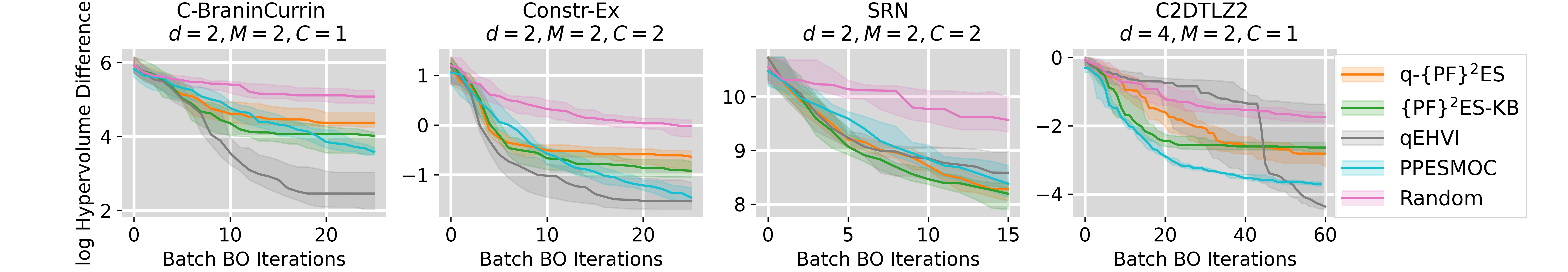
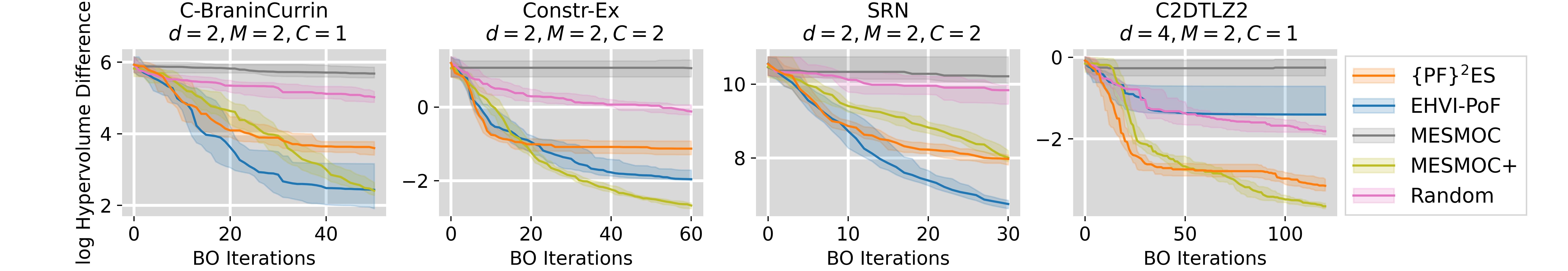
Figure 13: Comparison of different acquisition functions for multi-objective Bayesian optimization with respect to an in-sample recommendation strategy (In case of encountering a numerical issue (i.e., Cholesky decomposition issue), a different initial sample set is utilized.).

Appendix I ADDITIONAL EXPERIMENTAL RESULTS

I.1 Experimental results for the in-sample recommendation strategy

We report the experimental results of the in-sample recommendation strategy in the main paper, see Fig. 13, the in sampled Pareto frontiers are extracted from all of the data obtained so far in the current iteration. However, the in-sample recommendation strategy is not the intrinsic strategy for non-myopic information-theoretic acquisition functions.

I.2 Experimental results for larger batch sizes

Additional experimental results for larger batch sizes $q$ is given in Fig. 14. Besides the ZDT1 and C2DTLZ2 synthetic functions reported in the main paper, we also add the results of two new synthetic experiments, namely the DTLZ4 problem and the Osy problem, see Table 1 for detailed settings. In general, with the same black box function evaluation budget, q-{PF}²ES demonstrates similar performance. It is also expected that with an increase in batch size, the acquisition function performance can be degraded slightly due to the increasing complexity of the acquisition function optimization process.

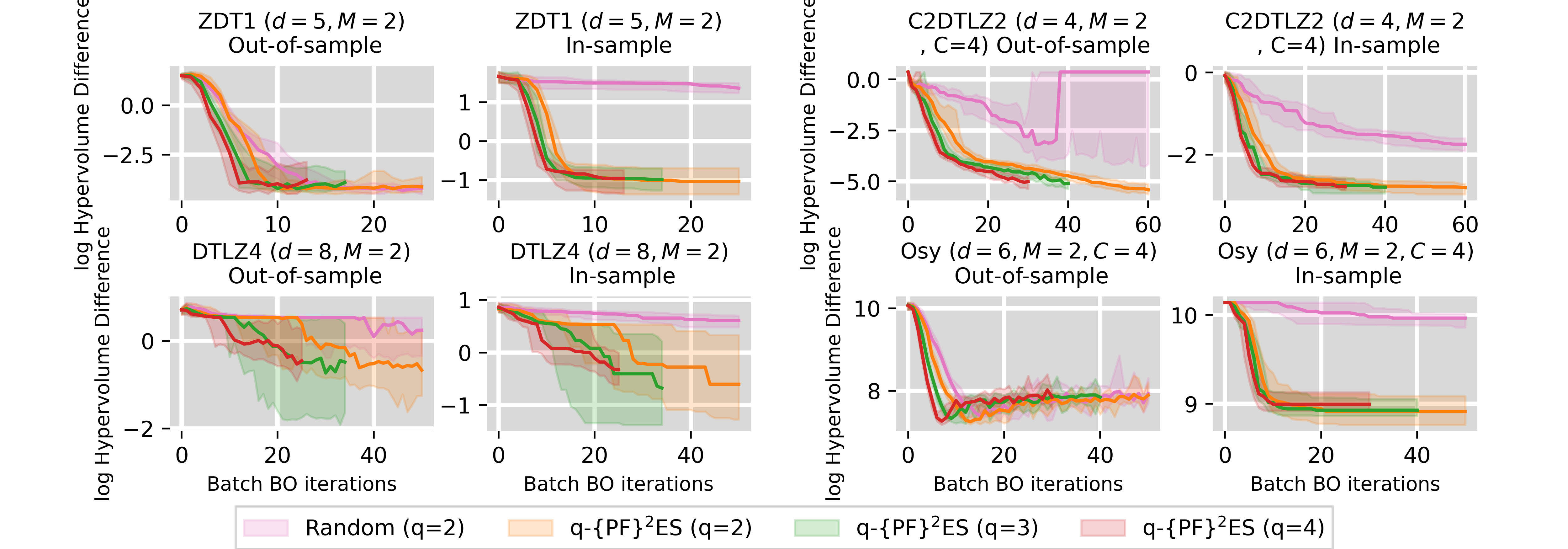
Figure 14: Numerical experiments of q-{PF}²ES on larger batch sizes. Note all the batch methods terminate on roughly the same number of function evaluations.

I.3 Experimental results for $M>2$ objectives

Two additional results for a larger number of objectives are seen in Fig. 15 based on two new problems. For the unconstrained version, we use DTLZ4 with 3 objective functions. For the constraint case, we use a real-life conceptual Marine design problem (Parsons and Scott,, 2004; Tanabe and Ishibuchi,, 2020). Details of the problem are also provided in Table 1. It can be observed that {PF}²ES and q-{PF}²ES provide competitive performance. For the conceptual Marine design problem, we generally observe that {PF}²ES-KB provides the fastest converge speed. We reason this is because given the relatively high constraint numbers, the approximated non-dominated feasible region $\tilde{A}$ is relatively small. For Monte Carlo-based acquisition functions like q-{PF}²ES, this can impose difficulties for approximation and optimization since $Z_{\tilde{A}_{q}}$ (Eq. 20) is rather small.

Note that, as discussed in Appendix. G, the computational complexity for providing the exact approximation of $A$ will increase exponentially with the number of objectives $M$, meaning that it will become the dominant factor in the calculation cost of {PF}²ES as $M$ increases. This is a common problem for hypervolume partition strategy-based acquisition functions (e.g., EHVI, MOPI).

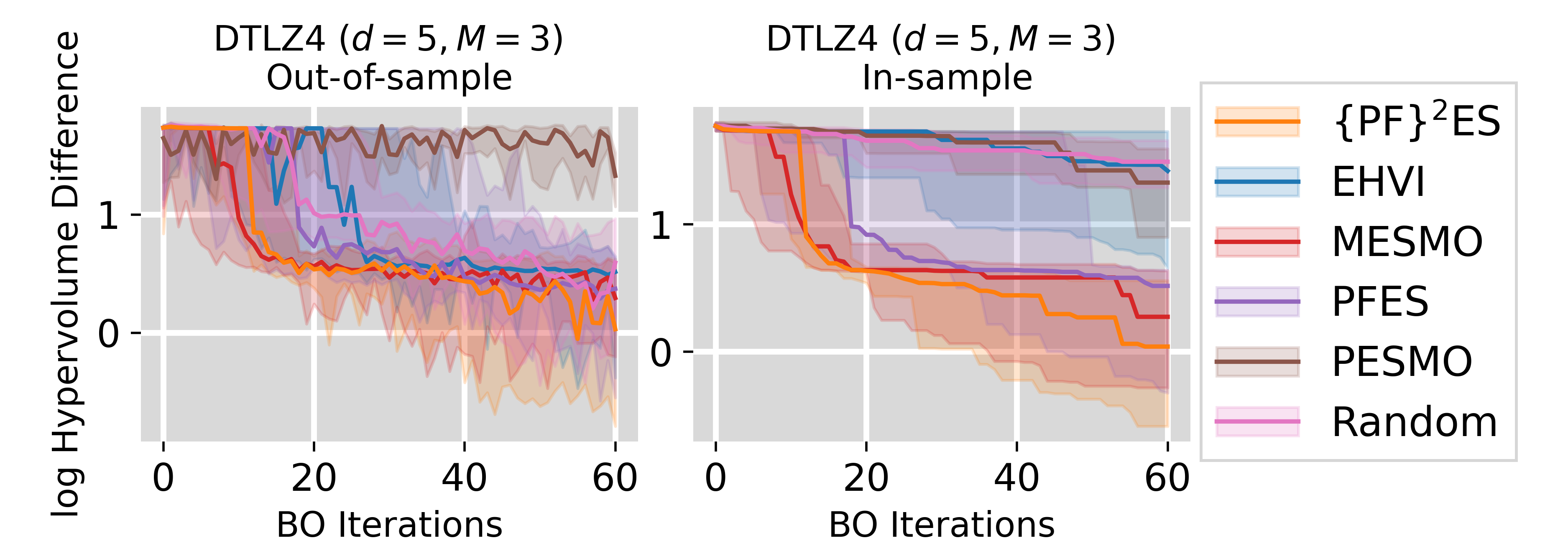
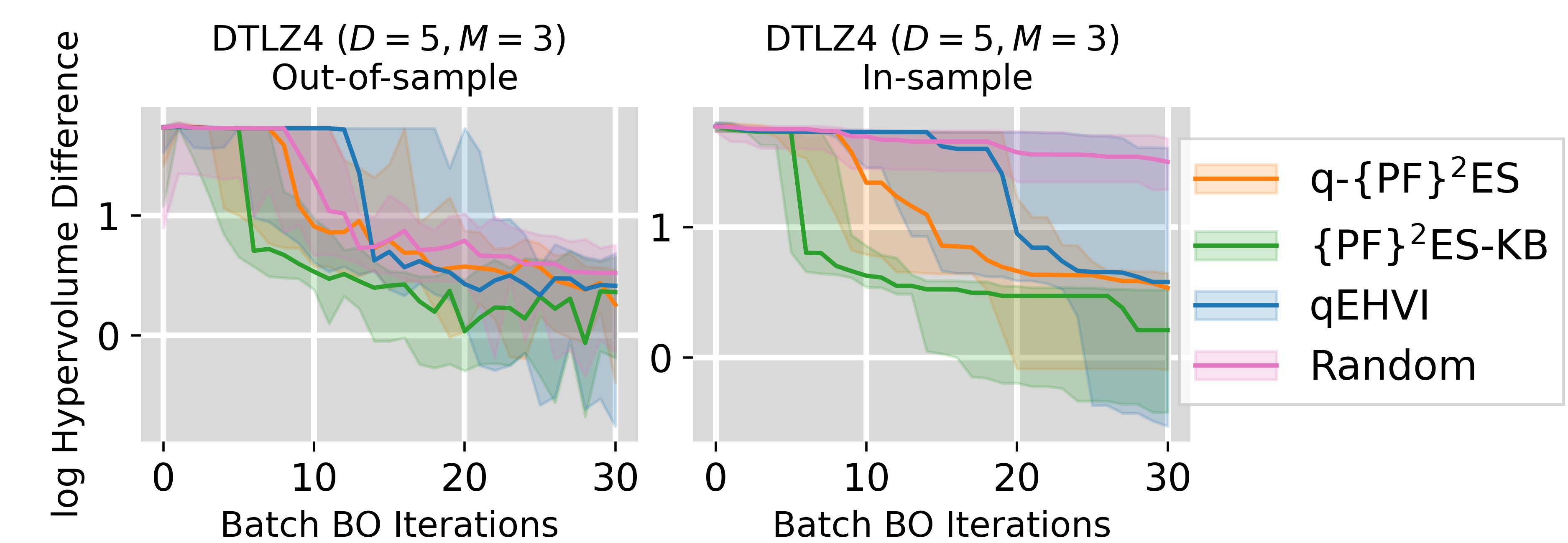
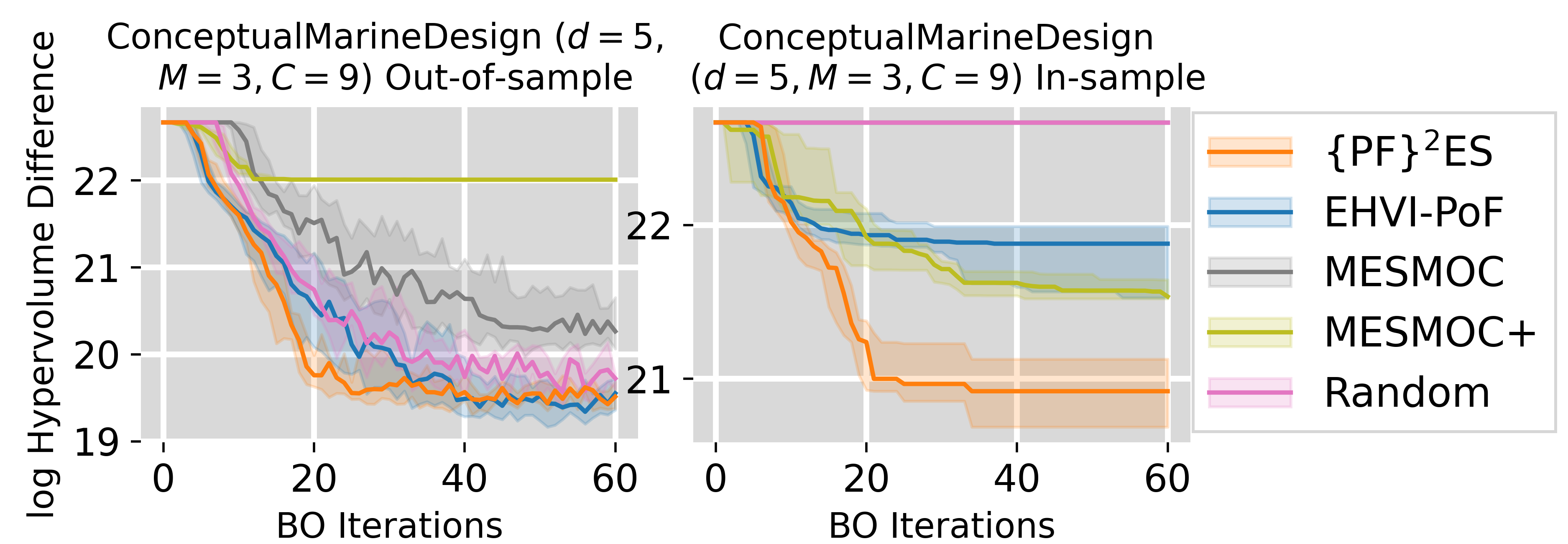
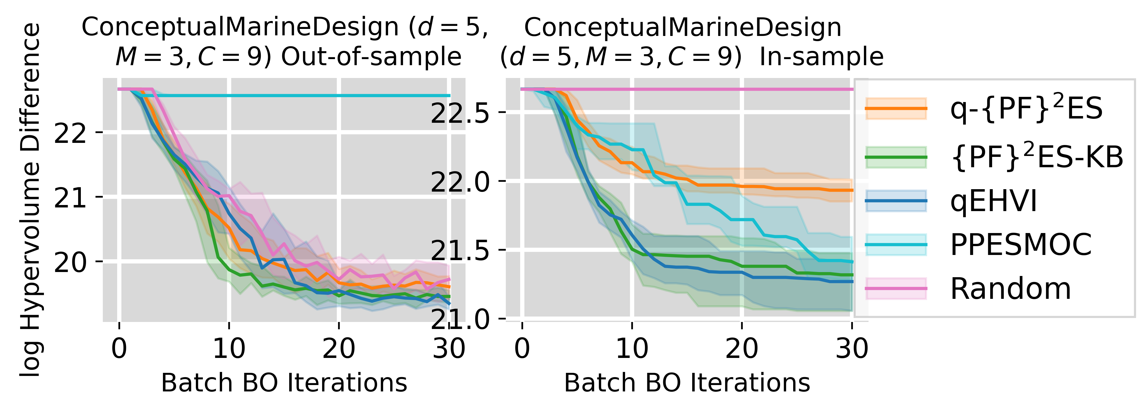
Figure 15: Experimental comparison for larger output dimensionality.

References

- Abdolshah et al., (2018) Abdolshah, M., Shilton, A., Rana, S., Gupta, S., and Venkatesh, S. (2018). Expected hypervolume improvement with constraints. In 2018 24th International Conference on Pattern Recognition (ICPR), pages 3238–3243. IEEE.
- Balandat et al., (2020) Balandat, M., Karrer, B., Jiang, D., Daulton, S., Letham, B., Wilson, A. G., and Bakshy, E. (2020). Botorch: a framework for efficient monte-carlo bayesian optimization. Advances in neural information processing systems, 33:21524–21538.
- Belakaria and Deshwal, (2019) Belakaria, S. and Deshwal, A. (2019). Max-value entropy search for multi-objective bayesian optimization. In International Conference on Neural Information Processing Systems (NeurIPS).
- Belakaria et al., (2020) Belakaria, S., Deshwal, A., and Doppa, J. R. (2020). Max-value entropy search for multi-objective bayesian optimization with constraints. arXiv preprint arXiv:2009.01721.
- Belakaria et al., (2021) Belakaria, S., Deshwal, A., and Doppa, J. R. (2021). Output space entropy search framework for multi-objective bayesian optimization. Journal of Artificial Intelligence Research, 72:667–715.
- Berkeley et al., (2022) Berkeley, J., Moss, H. B., Artemev, A., Pascual-Diaz, S., Granta, U., Stojic, H., Couckuyt, I., Qing, J., Loka, N., Paleyes, A., Ober, S. W., Goodall, A., Ghani, K., and Picheny, V. (2022). Trieste.
- Blank and Deb, (2020) Blank, J. and Deb, K. (2020). pymoo: Multi-objective optimization in python. IEEE Access, 8:89497–89509.
- Couckuyt et al., (2012) Couckuyt, I., Deschrijver, D., and Dhaene, T. (2012). Towards efficient multiobjective optimization: Multiobjective statistical criterions. 2012 IEEE Congress on Evolutionary Computation, CEC 2012, pages 10–15.
- Couckuyt et al., (2014) Couckuyt, I., Deschrijver, D., and Dhaene, T. (2014). Fast calculation of multiobjective probability of improvement and expected improvement criteria for pareto optimization. Journal of Global Optimization, 60(3):575–594.
- Cover, (1999) Cover, T. M. (1999). Elements of information theory. John Wiley & Sons.
- Dauert, (1993) Dauert, J. (1993). Multicriteria optimization in engineering: a tutorial and survey. Progress In Astronautics and Aeronautics: Structural Optimization: Status and Promise, 150:209.
- Daulton et al., (2020) Daulton, S., Balandat, M., and Bakshy, E. (2020). Differentiable expected hypervolume improvement for parallel multi-objective bayesian optimization. arXiv preprint arXiv:2006.05078.
- Daulton et al., (2021) Daulton, S., Balandat, M., and Bakshy, E. (2021). Parallel bayesian optimization of multiple noisy objectives with expected hypervolume improvement. Advances in Neural Information Processing Systems, 34.
- Daulton et al., (2022) Daulton, S., Eriksson, D., Balandat, M., and Bakshy, E. (2022). Multi-objective bayesian optimization over high-dimensional search spaces. In Uncertainty in Artificial Intelligence, pages 507–517. PMLR.
- Deb, (2019) Deb, K. (2019). Constrained multi-objective evolutionary algorithm. In Evolutionary and Swarm Intelligence Algorithms, pages 85–118. Springer.
- Deb and Agrawal, (1999) Deb, K. and Agrawal, S. (1999). A niched-penalty approach for constraint handling in genetic algorithms. In Artificial neural nets and genetic algorithms, pages 235–243. Springer.
- Deb and Kalyanmoy, (2001) Deb, K. and Kalyanmoy, D. (2001). Multi-Objective Optimization Using Evolutionary Algorithms. John Wiley & Sons, Inc., USA.
- Deb et al., (2002) Deb, K., Pratap, A., Agarwal, S., and Meyarivan, T. (2002). A fast and elitist multiobjective genetic algorithm: Nsga-ii. IEEE transactions on evolutionary computation, 6(2):182–197.
- Deb et al., (2005) Deb, K., Thiele, L., Laumanns, M., and Zitzler, E. (2005). Scalable test problems for evolutionary multiobjective optimization. In Evolutionary multiobjective optimization, pages 105–145. Springer.
- Emmerich and Deutz, (2018) Emmerich, M. and Deutz, A. H. (2018). A tutorial on multiobjective optimization: fundamentals and evolutionary methods. Natural computing, 17(3):585–609.
- Emmerich et al., (2020) Emmerich, M., Yang, K., and Deutz, A. H. (2020). Infill criteria for multiobjective bayesian optimization. In High-Performance Simulation-Based Optimization, pages 3–16. Springer.
- Feliot et al., (2017) Feliot, P., Bect, J., and Vazquez, E. (2017). A bayesian approach to constrained single-and multi-objective optimization. Journal of Global Optimization, 67(1):97–133.
- Fernández-Sánchez et al., (2020) Fernández-Sánchez, D., Garrido-Merchán, E. C., and Hernández-Lobato, D. (2020). Max-value entropy search for multi-objective bayesian optimization with constraints. arXiv e-prints, pages arXiv–2011.
- Frazier, (2018) Frazier, P. I. (2018). A tutorial on bayesian optimization. arXiv preprint arXiv:1807.02811.
- Gardner et al., (2014) Gardner, J. R., Kusner, M. J., Xu, Z. E., Weinberger, K. Q., and Cunningham, J. P. (2014). Bayesian optimization with inequality constraints. In ICML, volume 2014, pages 937–945.
- Garnett, (2022) Garnett, R. (2022). Bayesian Optimization. Cambridge University Press. in preparation.
- Garrido-Merchán and Hernández-Lobato, (2019) Garrido-Merchán, E. C. and Hernández-Lobato, D. (2019). Predictive entropy search for multi-objective bayesian optimization with constraints. Neurocomputing, 361:50–68.
- Garrido-Merchán and Hernández-Lobato, (2020) Garrido-Merchán, E. C. and Hernández-Lobato, D. (2020). Parallel predictive entropy search for multi-objective bayesian optimization with constraints. arXiv preprint arXiv:2004.00601.
- Ginsbourger et al., (2010) Ginsbourger, D., Riche, R. L., and Carraro, L. (2010). Kriging is well-suited to parallelize optimization. In Computational intelligence in expensive optimization problems, pages 131–162. Springer.
- Guerreiro et al., (2020) Guerreiro, A. P., Fonseca, C. M., and Paquete, L. (2020). The hypervolume indicator: Problems and algorithms. arXiv preprint arXiv:2005.00515.
- Hawe and Sykulski, (2008) Hawe, G. and Sykulski, J. (2008). Probability of improvement methods for constrained multi-objective optimization. In 2008 IET 7th International Conference on Computation in Electromagnetics, pages 50–51. IET.
- Hawe and Sykulski, (2007) Hawe, G. I. and Sykulski, J. K. (2007). An enhanced probability of improvement utility function for locating pareto optimal solutions.
- Hennig and Schuler, (2012) Hennig, P. and Schuler, C. J. (2012). Entropy search for information-efficient global optimization. Journal of Machine Learning Research, 13(6).
- Hernández-Lobato et al., (2016) Hernández-Lobato, D., Hernández-Lobato, J., Shah, A., and Adams, R. (2016). Predictive entropy search for multi-objective bayesian optimization. In International Conference on Machine Learning, pages 1492–1501. PMLR.
- Hernández-Lobato et al., (2014) Hernández-Lobato, J. M., Hoffman, M. W., and Ghahramani, Z. (2014). Predictive entropy search for efficient global optimization of black-box functions. Advances in neural information processing systems, 27.
- Hvarfner et al., (2022) Hvarfner, C., Hutter, F., and Nardi, L. (2022). Joint entropy search for maximally-informed bayesian optimization. arXiv preprint arXiv:2206.04771.
- Kingma and Welling, (2013) Kingma, D. P. and Welling, M. (2013). Auto-encoding variational bayes. arXiv preprint arXiv:1312.6114.
- Knudde et al., (2017) Knudde, N., van der Herten, J., Dhaene, T., and Couckuyt, I. (2017). Gpflowopt: A bayesian optimization library using tensorflow. arXiv preprint arXiv:1711.03845.
- Kushner, (1964) Kushner, H. J. (1964). A new method of locating the maximum point of an arbitrary multipeak curve in the presence of noise.
- Lacour et al., (2017) Lacour, R., Klamroth, K., and Fonseca, C. M. (2017). A box decomposition algorithm to compute the hypervolume indicator. Computers & Operations Research, 79:347–360.
- Martínez-Frutos and Herrero-Pérez, (2016) Martínez-Frutos, J. and Herrero-Pérez, D. (2016). Kriging-based infill sampling criterion for constraint handling in multi-objective optimization. Journal of Global Optimization, 64(1):97–115.
- Moss et al., (2021) Moss, H. B., Leslie, D. S., Gonzalez, J., and Rayson, P. (2021). Gibbon: General-purpose information-based bayesian optimisation. arXiv preprint arXiv:2102.03324.
- Osyczka and Kundu, (1995) Osyczka, A. and Kundu, S. (1995). A new method to solve generalized multicriteria optimization problems using the simple genetic algorithm. Structural optimization, 10(2):94–99.
- Parsons and Scott, (2004) Parsons, M. G. and Scott, R. L. (2004). Formulation of multicriterion design optimization problems for solution with scalar numerical optimization methods. Journal of Ship Research, 48(01):61–76.
- Poole et al., (2019) Poole, B., Ozair, S., Van Den Oord, A., Alemi, A., and Tucker, G. (2019). On variational bounds of mutual information. In International Conference on Machine Learning, pages 5171–5180. PMLR.
- (46) Qing, J., Couckuyt, I., and Dhaene, T. (2022a). A robust multi-objective bayesian optimization framework considering input uncertainty. arXiv preprint arXiv:2202.12848.
- (47) Qing, J., Dhaene, T., and Couckuyt, I. (2022b). Spectral representation of robustness measures for optimization under input uncertainty. In ICML2022, the 39th International Conference on Machine Learning, pages 1–26.
- Qing et al., (2021) Qing, J., Knudde, N., Garbuglia, F., Spina, D., Couckuyt, I., and Dhaene, T. (2021). Adaptive sampling with automatic stopping for feasible region identification in engineering design. Engineering with Computers, pages 1–18.
- Rahimi and Recht, (2007) Rahimi, A. and Recht, B. (2007). Random features for large-scale kernel machines. Advances in neural information processing systems, 20.
- Rasmussen, (2003) Rasmussen, C. E. (2003). Gaussian processes in machine learning. In Summer school on machine learning, pages 63–71. Springer.
- Ray and Liew, (2002) Ray, T. and Liew, K. (2002). A swarm metaphor for multiobjective design optimization. Engineering optimization, 34(2):141–153.
- Schubert et al., (2017) Schubert, E., Sander, J., Ester, M., Kriegel, H. P., and Xu, X. (2017). Dbscan revisited, revisited: why and how you should (still) use dbscan. ACM Transactions on Database Systems (TODS), 42(3):1–21.
- Shahriari et al., (2015) Shahriari, B., Swersky, K., Wang, Z., Adams, R. P., and De Freitas, N. (2015). Taking the human out of the loop: A review of bayesian optimization. Proceedings of the IEEE, 104(1):148–175.
- Srinivas and Deb, (1994) Srinivas, N. and Deb, K. (1994). Muiltiobjective optimization using nondominated sorting in genetic algorithms. Evol. Comput., 2(3):221–248.
- Suzuki et al., (2020) Suzuki, S., Takeno, S., Tamura, T., Shitara, K., and Karasuyama, M. (2020). Multi-objective bayesian optimization using pareto-frontier entropy. In International Conference on Machine Learning, pages 9279–9288. PMLR.
- Takeno et al., (2022) Takeno, S., Tamura, T., Shitara, K., and Karasuyama, M. (2022). Sequential and parallel constrained max-value entropy search via information lower bound. In International Conference on Machine Learning, pages 20960–20986. PMLR.
- Tanabe and Ishibuchi, (2020) Tanabe, R. and Ishibuchi, H. (2020). An easy-to-use real-world multi-objective optimization problem suite. Applied Soft Computing, 89:106078.
- Ungredda and Branke, (2021) Ungredda, J. and Branke, J. (2021). Bayesian optimisation for constrained problems. arXiv preprint arXiv:2105.13245.
- Vakili et al., (2020) Vakili, S., Picheny, V., and Durrande, N. (2020). Regret bounds for noise-free bayesian optimization. arXiv preprint arXiv:2002.05096.
- Van Veldhuizen and Lamont, (1999) Van Veldhuizen, D. A. and Lamont, G. B. (1999). Multiobjective evolutionary algorithm test suites. In Proceedings of the 1999 ACM symposium on Applied computing, pages 351–357.
- Wang and Jegelka, (2017) Wang, Z. and Jegelka, S. (2017). Max-value entropy search for efficient Bayesian optimization. In Precup, D. and Teh, Y. W., editors, Proceedings of the 34th International Conference on Machine Learning, volume 70 of Proceedings of Machine Learning Research, pages 3627–3635. PMLR.
- Wang et al., (2016) Wang, Z., Zhou, B., and Jegelka, S. (2016). Optimization as estimation with gaussian processes in bandit settings. In Artificial Intelligence and Statistics, pages 1022–1031. PMLR.
- Wilson et al., (2018) Wilson, J., Hutter, F., and Deisenroth, M. (2018). Maximizing acquisition functions for bayesian optimization. Advances in neural information processing systems, 31.
- Yang et al., (2019) Yang, K., Emmerich, M., Deutz, A., and Bäck, T. (2019). Efficient computation of expected hypervolume improvement using box decomposition algorithms. Journal of Global Optimization, 75(1):3–34.
- Zitzler et al., (2000) Zitzler, E., Deb, K., and Thiele, L. (2000). Comparison of multiobjective evolutionary algorithms: Empirical results. Evolutionary computation, 8(2):173–195.