Supplemental Material
Tissue fluidization by cell-shape-controlled active stresses

I Simulation implementation

I.1 Simulation setup and parameter values

The cell dynamics is dictated by the motions of vertices, which obey the force balance equation (Eq. (2) in the main text). In addition, we implemented T1 transitions once the length of a cell edge decreases below a critical value $\Delta_{\rm T1}$ Fletcher et al. (2014); Bi et al. (2015); Lin et al. (2018).

Simulations were started from a regular hexagonal pattern (or random Voronoi pattern if stated) with small Gaussian perturbations (magnitude = 0.01) applied to the vertices’ positions at $t=0$, and run for enough steps (typically $N_{\rm simulation}=100,000$) to arrive dynamic steady state, which can be checked by examining the evolutions of the cell elongation parameter $q$, the hexatic order parameter $\psi_{6}$, the average vertex coordination number $Z$, see Fig. S1 for example. We systematically consider system prepared with zero residual stress (see Sec. I.2).

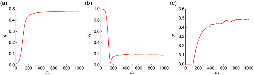
FIG. S1: An example to check the dynamic steady state. Evolutions of (a) the cell elongation parameter $q$, (b) the hexatic order parameter $\psi_{6}$, and (c) the average vertex coordination number $Z$. Parameters: $K_{P}=0.02$, $P_{0}=1.0$ and $\beta=0.3$.

In our simulations, the governing equations and corresponding parameters are rescaled by the length scale $\ell=\sqrt{{{A}_{0}}}$, the time scale $\tau={\gamma}/{\left({{K}_{A}}{{A}_{0}}\right)}\;$, and the stress scale $\sigma={{K}_{A}}{{A}_{0}}$. The following non-dimensional parameter values are adopted: ${K}_{P}=0.02$, ${{\Delta}_{\text{T}1}}=0.01$, and $\Delta t=0.01$. If not stated otherwise, we consider a system of $N_{\rm cell}=1,000$ and an initially hexagonal cell pattern. In Sec. III.2, we verified that our results were consistent for a wide range of system sizes.

I.2 Generation of a global stress-free cell sheet

The stress-free configuration is defined as a configuration where the global tissue stress is zero. We here give the details of how to generate the stress-free configuration for a cell sheet without active stress.

Once we set up a hexagonal cell pattern or random Voronoi cell pattern, we compute the global stress in the cell sheet. It is possible to compute cell-based stresses from the forces applied on the vertices using the Batchelor formula Batchelor (1970); Lau and Lubensky (2009); Nestor-Bergmann et al. (2018). In the absence of active stress, the cell stress can be expressed as:

$$\bm{\sigma}_{J}=\left[{{K}_{A}}\left(A_{J}-{{A}_{0}}\right)+\frac{1}{2}\frac{{{K}_{P}}P_{J}\left(P_{J}-{{P}_{0}}\right)}{A_{J}}\right]\bm{I}+\frac{{{K}_{P}}P_{J}\left(P_{J}-{{P}_{0}}\right)}{A_{J}}\bm{Q}_{J},$$ (S1)

where the first term is the isotropic stress and the second term is the anisotropic stress. The global stress in a cell sheet can be calculated by, ${{\bm{\sigma}}^{\left(\text{tissue}\right)}}\left[\{\bm{r}_{i}\}\right]={\sum_{J}{{{A}_{J}}{{\bm{\sigma}}_{J}}}}/{\sum_{J}{{{A}_{J}}}}$.

The initial tissue state correspond to a global stress $\bm{\sigma}^{\rm(tissue)}$ that is non-zero. Here we propose a two-step protocol to achieve a near zero-stress state.

1. As a first step, we apply a uniform affine transformation to the cell sheet, $\{\bm{r}_{i}\}\rightarrow\{\lambda\bm{r}_{i}\}$, where $\lambda>0$ here is a scaling factor to be determined in the following. In the new configuration, $\{\lambda\bm{r}_{i}\}$, the global stress in the tissue can be expressed as

   $${{\bm{\sigma}}^{\left(\text{tissue}\right)}}\left[\left\{\lambda{{\bm{r}}_{i}}\right\}\right]=\frac{\sum\limits_{J}{\left\{\left[\lambda{{K}_{A}}{{A}_{J}}\left({{\lambda}^{2}}{{A}_{J}}-{{A}_{0}}\right)+\dfrac{1}{2}{{K}_{P}}{{P}_{J}}\left(\lambda{{P}_{J}}-{{P}_{0}}\right)\right]\bm{I}+{{K}_{P}}{{P}_{J}}\left(\lambda{{P}_{J}}-{{P}_{0}}\right){{\bm{Q}}_{J}}\right\}}}{\lambda\sum\limits_{J}{{{A}_{J}}}}.$$ (S2)

   To get the stress-free state, we first reach a traceless stress state through a rescaling factor $\lambda$ that solves the condition $\mathrm{tr}\{\bm{\sigma}^{(\rm tissue)}\big{[}\lambda\bm{r}_{i}\big{]}\}=0$, which reads

   $$\left(4\sum\limits_{J}{\tilde{A}_{J}^{2}}\right){{\lambda}^{3}}+\left(2{{{\tilde{K}}}_{P}}\sum\limits_{J}{\tilde{P}_{J}^{2}}-4\sum\limits_{J}{{{{\tilde{A}}}_{J}}}\right)\lambda-2{{\tilde{K}}_{P}}{{\tilde{P}}_{0}}\sum\limits_{J}{{{{\tilde{P}}}_{J}}}=0,$$ (S3)

   where ${{\tilde{K}}_{P}}={K}_{P}/({K}_{A}{A}_{0})$, ${{\tilde{P}}_{0}}={P}_{0}/\sqrt{{{A}_{0}}}$, ${{\tilde{A}}_{J}}={A}_{J}/{A}_{0}$, and ${{\tilde{P}}_{J}}={P}_{J}/\sqrt{{A}_{0}}$ are the dimensionless parameters.

2. Although Eq. (S3) does not strictly imply that $\bm{\sigma}^{(\rm tissue)}=\bm{0}$, such condition yields an initial tissue configuration that is relatively close to a zero stress state. To achieve such zero stress state, we let the system evolve through the classical vertex model simulation. We find that this is efficient to decrease the residual global tissue stress. At the end of the simulation, we evaluate whether the stress is small enough; more precisely, we check whether the maximal absolute component of the stress, denoted $|\bm{\sigma}^{(\rm tissue)}|$, is smaller than a threshold value set to $\sigma_{0}=0.01$, i.e. $|\bm{\sigma}^{(\rm tissue)}|<\sigma_{0}$. If the condition is met, we consider that a stress-free state is obtained; otherwise, we repeat the above steps, until the condition $|\bm{\sigma}^{(\rm tissue)}|<\sigma_{0}$ is met.

Our protocol was always found to converge.

I.3 Simple shear simulations

Our simple shear simulations are performed using the Lees–Edwards periodic boundary conditions (Fig. S2 and Bi et al. (2015); Merkel et al. (2019)). Note that before shearing, the cell sheet is relaxed to a steady state (see Fig. 1(b) in the main text for examples). In the following we detail our implementation protocol.

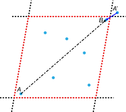
FIG. S2: Schematic of the Lees–Edwards periodic boundary conditions.

I.3.1 Lees–Edwards periodic boundary conditions

In the sheared configuration, the calculations of the relative position and distance of vertex (cell) pairs should obey the Lees–Edwards periodic boundary conditions, as shown in Fig. S2. For example, the position vector of the neighboring vertex pair $A$ and $B$, $\bm{r}_{A\rightarrow B}$, cannot be simply measured as $\bm{r}_{B}-\bm{r}_{A}$, but instead should be measured as $\bm{r}_{B}-\bm{r}_{A^{\prime}}$ with $A^{\prime}$ being the mirror of vertex $A$. Specifically, denote $\bm{r}_{A\rightarrow B}^{(0)}=\bm{r}_{B}-\bm{r}_{A}$, then $\bm{r}_{A\rightarrow B}=(x_{A\rightarrow B},y_{A\rightarrow B})$ can be calculated as

$$\begin{split}{{x}_{A\to B}}&=x_{A\to B}^{\left(0\right)}-{{L}_{x}}\mathcal{R}\left[\frac{x_{A\to B}^{\left(0\right)}-{{\gamma}_{xy}}y_{A\to B}^{\left(0\right)}}{{{L}_{x}}}\right]-{{\gamma}_{xy}}{{L}_{y}}\mathcal{R}\left[\frac{y_{A\to B}^{\left(0\right)}}{{{L}_{y}}}\right],\\ {{y}_{A\to B}}&=y_{A\to B}^{\left(0\right)}-{{L}_{y}}\mathcal{R}\left[\frac{y_{A\to B}^{\left(0\right)}}{{{L}_{y}}}\right],\end{split}$$ (S4)

where $\mathcal{R}\left[\cdot\right]$ represents the function round to nearest integer and $\gamma_{xy}$ is the simple shear strain.

I.3.2 Tissue under a constant simple shear strain

Definition

To examine the shear modulus of a cell sheet, we perform simple shear simulations as below:

1. First, we apply a small simple shear deformation $\gamma_{xy}=0.01\ll 1$ to the cell sheet by mapping all the vertices to new positions,

   $${{x}_{\text{new}}}=x+{{\gamma}_{xy}}y\quad,\quad{{y}_{\text{new}}}=y.$$ (S5)

2. Second, the simple shear strain is maintained for a sufficiently long time for the sheared configuration to relax. We keep track the global shear stress $\sigma_{xy}^{(\rm{tissue})}$ during the relaxation and check that the evolution of the global shear falls below a threshold value. The shear modulus of the cell sheet then reads

   $$G_{xy}=\frac{\langle\sigma_{xy}^{\left(\text{tissue}\right)}\rangle_{\rm A}-\langle\sigma_{xy}^{\left(\text{tissue}\right)}\rangle_{\rm B}}{{{\gamma}_{xy}}},$$ (S6)

   where $\langle\sigma_{xy}^{\left(\text{tissue}\right)}\rangle_{\rm B}$ and $\langle\sigma_{xy}^{\left(\text{tissue}\right)}\rangle_{\rm A}$ are the average tissue shear stress before and after simple shear strain, respectively.

Verification

We checked that, within the solid regime, the shear modulus is not significantly changed for a range of values $\gamma_{xy}=(0.001,0.10)$ for all considered $\beta$.

I.3.3 Tissue under quasi-statically increasing simple shear strain

Definition

We also perform simple shear simulations by a quasi-static increasing of the amplitude in the simple shear strain $\gamma_{xy}(t)$. The procedure is the following:

1. First, the simple shear strain is increased in a step-by-step fashion

   $$\gamma_{xy}^{\left(\text{new}\right)}={{\gamma}_{xy}}+\Delta{{\gamma}_{xy}},$$ (S7)

   where the incremental shear strain $\Delta\gamma_{xy}$ is small and set to be $\Delta\gamma_{xy}=0.01$ in our simulations.

2. Second, after updating the simple shear strain, vertices are mapped to new positions as

   $${{x}_{\text{new}}}=x_{\rm ref}+{{\gamma}_{xy}^{(\rm{new})}}y_{\rm ref}\quad,\quad{{y}_{\text{new}}}=y_{\rm ref},$$ (S8)

   where $x_{\rm ref}=x-\gamma_{xy}y$ and $y_{\rm ref}=y$ are the reference coordinates in the reference configuration without shear.

3. Third, the new simple shear strain is kept and the cell sheet is relaxed for a duration $\tau_{\rm relax}=100$. After relaxation, the global shear stress is computed to construct the stress-strain relation $\sigma_{xy}^{(\rm{tissue})}(\gamma_{xy})$ during such continuous shearing process.

We then repeat the above three steps up to a maximal strain set at $\gamma_{xy}=3.0$. The tissue-scale shear modulus can be estimated as the derivative at zero shear strain of the shear stress curve with respect to the initial shear strain.

Verification

We checked that the relaxation time $\tau_{\rm relax}=100$ after each step increase is sufficient long to provide stable estimates of the shear modulus and yield stress $\sigma_{\rm yield}$), see Sec. I.4.4.

I.4 Quantification

I.4.1 Coordination number $Z$

To quantify the coordination number $Z$ represented in Figure 1, we first (1) find clusters of vertices, denoted $C_{i}$, that are closer to one another than a threshold distance $0.01$ and (2) estimate the mean coordination number $Z=\sum_{C_{i}}N(C_{i})$ where $N(C_{i})$ is the number of vertices in the cluster $C_{i}$.

I.4.2 T1 transition rate

Definition

To quantify the dynamics of cell rearrangements, we examine the rate of T1 transitions after the system arrives at a dynamic steady state. We define the T1 transition rate as,

$$k_{\rm T1}=\frac{N_{\rm T1}}{N_{\rm cells}\tau},$$ (S9)

where $N_{\rm T1}$ is the total number of T1 transitions during the observation time $\tau$.

Localization of T1 transitions

We also examine the spatial distribution of T1 transitions, as shown in Fig. S3. It demonstrates that at the rhombile regime, T1 transitions are highly localized (with hotspots of frequent T1 transitions corresponding to cell-cell rearrangement oscillations) and sub-domains of rhombile patterns without any T1 transitions (see Movie S2). In the fluid regime $\beta=0.5$, T1 transitions are more uniformly distributed, indicating a completely disordered fluid regime.

Method for counting T1 transitions

We exclude repeated T1 transitions from the count of the T1 transition rate in the main text Figure 1. To exclude repeated T1 transitions, we keep track of the cells involved in each T1 transition and disregard any new T1 transitions that would involve the exact same set of cells as previously encountered. The number of T1 transition in Figure 1 was estimated over an observation time window of duration $\tau=100$ ending with simulations.

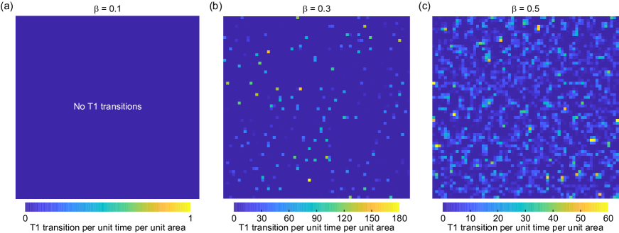
FIG. S3: The hotspot map of T1 transitions (including repeated ones). (a) $\beta=0.1$. (b) $\beta=0.3$. (c) $\beta=0.5$. Parameters: $K_{P}=0.02$, and $P_{0}=1.0$.

I.4.3 Bond-orientational correlation function

Definition

As in the main text, the tissue hexatic order parameter is defined as

$${{\psi}_{6}}\left(t\right)=\left|\frac{1}{N}\sum\limits_{j=1}^{N}{{{\Psi}_{j}}\left(t\right)}\right|,$$ (S10)

where ${{\Psi}_{j}}=\sum_{k\in\text{neighbors}}{\exp\left(\text{i}6{{\theta}_{jk}}\right)}/N_{j}$, with $\theta_{jk}=\arg\left(\bm{r}_{k}-\bm{r}_{j}\right)$ Li and Ciamarra (2018); Paoluzzi et al. (2021). To quantify the spatial correlation of tissue architecture, we compute the bond-orientational correlation function,

$${{g}_{6}}\left(r\right)=\frac{\left\langle{{\Psi}_{i}}\overline{{{\Psi}_{j}}}\right\rangle}{\left\langle{{\Psi}_{i}}\overline{{{\Psi}_{i}}}\right\rangle},$$ (S11)

where $\overline{\star}$ denotes the conjugate complex number and $r=|\bm{r}_{i}-\bm{r}_{j}|$.

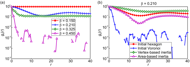
FIG. S4: The bond-orientational correlation function $g_{6}(r)$, defined by Eq. (S11). (a) $g_{6}(r)$ at different $\beta$ values, for initially hexagonal pattern. (b) Comparison of $g_{6}(r)$ for either the initially hexagonal pattern (red: standard $Q$ tensor; green: vertex-based inertia tensor; magenta: area-based inertia tensor) or the initially Voronoi pattern (blue: standard $Q$ tensor), at $\beta=0.210$. Parameters: $K_{P}=0.02$, $P_{0}=1$ and $N=10,000$ cells.

Results

Figure S4(a) shows the bond-orientational correlation function $g_{6}(r)$ for different values of $\beta$. For the solid regime with isotropic cells, $g_{6}(r)=1$; for both the solid regime with anisotropic cells and the rhombile regime, $g_{6}(r)$ decreases as $r$ is increased and approaches a finite positive value for large $r$, suggesting long-range orientational order when the tissue is initialized according to a near perfect hexagonal pattern. We confirm such result for the three different definitions of $\bm{Q}$. In contrast, when the tissue is initialized according to a Voronoi pattern, $g_{6}(r)$ decreases exponentially to zero. In the fluid regime $\beta>\beta_{3}$ (see main text), $g_{6}(r)$ decreases exponentially to zero at large $r$.

I.4.4 Yield shear stress

Definition

In Sec. I.3, we proposed a protocol to implement a quasi-static increase of a simple shear strain. We represent typical stress-strain curves for different values of $\beta$ for tissues either initialized in a near hexagonal state (Fig. S5(a)) or according to a Voronoi pattern (Fig. S5(c)). We define the yield stress $\sigma_{\rm yield}$ as the maximum of the shear stress $\sigma_{xy}$ curve. The yield stress is represented in the main text Figure 1(e).

Discussion

When the initial pattern is near hexagonal (Fig. S5(a)), the shear stress sharply drops beyond a critical yield strain. Such a sharp drop of $\sigma_{xy}$ is due to a large number of simultaneous T1 transitions. The curve is more smooth in the case for a tissue initialized according to a Voronoi pattern.

Verification

We check that the measured shear modulus and yield stress are insensitive to the relaxation time duration of simple shear strain increment in a broad range $10<\tau_{\rm relax}<1000$, Fig. S5(b).

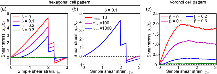
FIG. S5: The yield stress measurement. (a, b) Hexagonal cell pattern; (c) Voronoi cell pattern. (a, c) Curves of the shear stress $\sigma_{xy}$ versus the simple shear strain $\gamma_{xy}$ for different cell activities $\beta=0,\ 0.1,\ 0.2,\ 0.3$. Here the relaxation time $\tau_{\rm relax}=100$. (b) Curves of the shear stress $\sigma_{xy}$ versus the simple shear strain $\gamma_{xy}$ for different relaxation time $\tau_{\rm relax}=10,\ 100,\ 1000$ at $\beta=0.1$. Parameters: $K_{P}=0.02$ and $P_{0}=1.0$.

I.5 Simulation check for the passive case

Here we set $\beta=0$ (passive case) and check that our simulation framework agrees with previous studies Farhadifar et al. (2007); Bi et al. (2015); Sussman and Merkel (2018); Merkel et al. (2019); Wang et al. (2020). We first check it for an initially hexagonal cell pattern. We represent the cell elongation $q$ and shear modulus $G_{xy}$ as function of the target shape index $P_{0}$ in Fig. S6, which clearly indicates a shape and rigidity transition at $P_{0}^{\ast}\approx 3.723$. We also check it for an initially Voronoi cell pattern. Figure S6 shows that such a cell pattern undergoes a rigidity transition at $P_{0}^{\ast}\approx 3.846$.

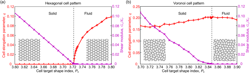
FIG. S6: Simulation of the rigidity transition in the passive vertex model. (a) Hexagonal cell pattern. (b) Voronoi cell pattern. Shown here are the cell elongation parameter $q$ and the (long-time) shear modulus $G_{xy}$ as a function of the cell target shape index $P_{0}$. Parameters: $K_{P}=0.02$ and $\beta=0$.

II Stability of the hexagonal pattern

II.1 Shape stability analysis of a single cell

Here we consider a regular hexagonal cell with shape-dependent active stress $\bm{\sigma}^{(\rm{act})}=-\beta\bm{Q}$ and ask whether the cell will elongate. To theoretically address such question, we consider a uniform deformation of the cell, as shown in Fig. S7. The cell deformation can be described by the stretches $\{\lambda_{1},\lambda_{2}\}$: $\{x_{i},y_{i}\}\rightarrow\{\lambda_{1}x_{i},\lambda_{2}y_{i}\}$, where $i$ is the index of cell vertices and $\lambda_{1}$ and $\lambda_{2}$ are cell stretches along $x$-axis and $y$-axis, respectively.

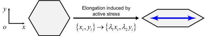
FIG. S7: Sketch of cell elongation induced by the cell shape-dependent active stress.

II.1.1 Equilibrium radius of a hexagonal cell without active stress

We first examine the equilibrium state of a hexagonal cell without active stress. We express the area and perimeter of the cell as $A=\frac{3\sqrt{3}}{2}{{R}^{2}}$ and $P=6R$ in terms of a quantity $R$, that we call the cell radius. We define the dimensionless equilibrium cell radius $\tilde{R}_{\rm h}=R_{\rm h}/\sqrt{A_{0}}$ as the solution of the mechanical equilibrium condition $\bm{\sigma}=\bm{0}$, which reads

$$\frac{9}{4}\tilde{R}_{\text{h}}^{3}+\left(6{{{\tilde{K}}}_{P}}-\frac{\sqrt{3}}{2}\right){{\tilde{R}}_{\text{h}}}-{{\tilde{K}}_{P}}{{\tilde{P}}_{0}}=0,$$ (S12)

In the incompressible limit case, i.e., $\tilde{K}_{P}\ll 1$, the equilibrium cell radius can be easily computed as $\tilde{R}_{\rm h}\simeq{\sqrt{2\sqrt{3}}}/{3}\approx 0.6204$.

II.1.2 Equilibrium configuration of a hexagonal cell with active stress

We now consider the effect of an active stress $\bm{\sigma}^{(\rm{act})}=-\beta\bm{Q}$, in which case the total cell stress reads

$$\bm{\sigma}=\left[{{K}_{A}}\left(A-{{A}_{0}}\right)+\frac{1}{2}\frac{{{K}_{P}}P\left(P-{{P}_{0}}\right)}{A}\right]\bm{I}+\left[\frac{{{K}_{P}}P\left(P-{{P}_{0}}\right)}{A}-\beta\right]\bm{Q}.$$ (S13)

Under an affine deformation:

$$\left\{{{x}_{i}},{{y}_{i}}\right\}\to\left\{{{\lambda}_{1}}{{x}_{i}},{{\lambda}_{2}}{{y}_{i}}\right\},$$ (S14)

the cell area, perimeter and anisotropy tensor of an initially hexagonal cell read

$$A =\frac{3\sqrt{3}}{2}R_{\text{h}}^{2}{{\lambda}_{1}}{{\lambda}_{2}},$$ (S15)

$$P =2{{R}_{\text{h}}}\left({{\lambda}_{1}}+\sqrt{\lambda_{1}^{2}+3\lambda_{2}^{2}}\right),$$ (S16)

$$\bm{Q} =\left(\frac{{{\lambda}_{1}}}{\sqrt{\lambda_{1}^{2}+3\lambda_{2}^{2}}}-\frac{1}{2}\right){{\bm{e}}_{x}}\otimes{{\bm{e}}_{x}}-\left(\frac{{{\lambda}_{1}}}{\sqrt{\lambda_{1}^{2}+3\lambda_{2}^{2}}}-\frac{1}{2}\right){{\bm{e}}_{y}}\otimes{{\bm{e}}_{y}}.$$ (S17)

The equilibrium state $\left\{\lambda_{1},\lambda_{2}\right\}$ of a cell corresponds to $\bm{\sigma}=\bm{0}$. Substituting the expressions of $A$, $P$ and $\bm{Q}$ into Eq. (S13), the condition $\bm{\sigma}=\bm{0}$ leads to:

$$\left(\frac{3\sqrt{3}}{2}\tilde{R}_{\text{h}}^{2}{{\lambda}_{1}}{{\lambda}_{2}}-1\right){{\lambda}_{2}}\sqrt{\lambda_{1}^{2}+3\lambda_{2}^{2}}-\frac{1}{2}{{\lambda}_{2}}\left(2{{\lambda}_{1}}-\sqrt{\lambda_{1}^{2}+3\lambda_{2}^{2}}\right)\tilde{\beta}$$

$$+\frac{4{{{\tilde{K}}}_{P}}}{3\sqrt{3}}\left({{\lambda}_{1}}+\sqrt{\lambda_{1}^{2}+3\lambda_{2}^{2}}\right)\left[2\left({{\lambda}_{1}}+\sqrt{\lambda_{1}^{2}+3\lambda_{2}^{2}}\right)-\frac{{{{\tilde{P}}}_{0}}}{{{{\tilde{R}}}_{\text{h}}}}\right]=0,$$ (S18)

$$\left(\frac{3\sqrt{3}}{2}\tilde{R}_{\text{h}}^{2}{{\lambda}_{1}}{{\lambda}_{2}}-1\right){{\lambda}_{1}}\sqrt{\lambda_{1}^{2}+3\lambda_{2}^{2}}+\frac{1}{2}{{\lambda}_{1}}\left(2{{\lambda}_{1}}-\sqrt{\lambda_{1}^{2}+3\lambda_{2}^{2}}\right)\tilde{\beta}$$

$$+\frac{4{{{\tilde{K}}}_{P}}}{\sqrt{3}}{{\lambda}_{2}}\left[2\left({{\lambda}_{1}}+\sqrt{\lambda_{1}^{2}+3\lambda_{2}^{2}}\right)-\frac{{{{\tilde{P}}}_{0}}}{{{{\tilde{R}}}_{\text{h}}}}\right]=0.$$ (S19)

where $\tilde{\beta}={\beta}/({{{K}_{A}}{{A}_{0}}})$ corresponds to the dimensionless strength of the active stress. Equations (S18) and (S19) shows that $\{\lambda_{1},\lambda_{2}\}=\{1,1\}$ is always one of the equilibrium state of the single cell system for arbitrary $\beta$. Yet increasing $\beta$, the system undergoes a pitchfork bifurcation and the cell start to elongate, as shown in Fig. S8.

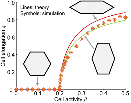
FIG. S8: Comparison of the elongation parameter $q$ of a hexagonal cell versus the cell activity $\beta$ between theoretical predictions (exact solutions given by solving Eqs. (S18) and (S19)) and single-cell simulations. Parameters: $\tilde{K}_{P}=0.02$ and $\tilde{P}_{0}=1$ (which results in an estimated transition at $\tilde{\beta}_{1}\approx 0.1987$ according to our theoretical prediction Eq. (S25)).

II.1.3 Stability analysis of a hexagonal cell

Now we turn to examine the stability of the equilibrium state $\{\lambda_{1}^{({\rm eq})},\lambda_{2}^{({\rm eq})}\}=\{1,1\}$ (i.e. a regular hexagon at equilibrium radius $R_{h}$) upon varying $\beta$. The first-order variation of the energy of the single cell system reads

$$\text{ }\!\!\delta\!\!\text{ }W=\frac{1}{2}\left(\text{ }\!\!\delta\!\!\text{ }A\bm{\sigma}:\bm{\varepsilon}+A\text{ }\!\!\delta\!\!\text{ }\bm{\sigma}:\bm{\varepsilon}+A\bm{\sigma}:\text{ }\!\!\delta\!\!\text{ }\bm{\varepsilon}\right).$$ (S20)

At the equilibrium state $\{\lambda_{1}^{({\rm eq})},\lambda_{2}^{({\rm eq})}\}=\{1,1\}$, ${{\left.\text{ }\!\!\delta\!\!\text{ }W\right|}_{\left\{1,1\right\}}}=0$. Further, the second-order variation of the energy reads

$${{\text{ }\!\!\delta\!\!\text{ }}^{2}}W=\text{ }\!\!\delta\!\!\text{ }A\text{ }\!\!\delta\!\!\text{ }\bm{\sigma}:\bm{\varepsilon}+\text{ }\!\!\delta\!\!\text{ }A\bm{\sigma}:\text{ }\!\!\delta\!\!\text{ }\bm{\varepsilon}+A\text{ }\!\!\delta\!\!\text{ }\bm{\sigma}:\text{ }\!\!\delta\!\!\text{ }\bm{\varepsilon}.$$ (S21)

At the equilibrium state $\{\lambda_{1}^{({\rm eq})},\lambda_{2}^{({\rm eq})}\}=\{1,1\}$, the latter equation reads

$${{\left.{{\text{ }\!\!\delta\!\!\text{ }}^{2}}W\right|}_{\left\{1,1\right\}}}={{\left.A\right|}_{\left\{1,1\right\}}}{{\left.\text{ }\!\!\delta\!\!\text{ }\bm{\sigma}\right|}_{\left\{1,1\right\}}}:{{\left.\text{ }\!\!\delta\!\!\text{ }\bm{\varepsilon}\right|}_{\left\{1,1\right\}}}={{\left.A\right|}_{\left\{1,1\right\}}}\left({{\varepsilon}_{1}},{{\varepsilon}_{2}}\right){{J}_{\sigma}}{{\left({{\varepsilon}_{1}},{{\varepsilon}_{2}}\right)}^{\text{T}}},$$ (S22)

where

$${{J}_{\sigma}}=\left(\begin{matrix}\dfrac{3\sqrt{3}}{2}{{K}_{A}}R_{\text{h}}^{2}+{{K}_{P}}\left(3\sqrt{3}-\dfrac{{{P}_{0}}}{2\sqrt{3}{{R}_{\text{h}}}}\right)-\dfrac{3}{8}\beta&\dfrac{3\sqrt{3}}{2}{{K}_{A}}R_{\text{h}}^{2}+{{K}_{P}}\left(-3\sqrt{3}+\dfrac{5{{P}_{0}}}{2\sqrt{3}{{R}_{\text{h}}}}\right)+\dfrac{3}{8}\beta\\ \dfrac{3\sqrt{3}}{2}{{K}_{A}}R_{\text{h}}^{2}+{{K}_{P}}\left(-3\sqrt{3}+\dfrac{5{{P}_{0}}}{2\sqrt{3}{{R}_{\text{h}}}}\right)+\dfrac{3}{8}\beta&\dfrac{3\sqrt{3}}{2}{{K}_{A}}R_{\text{h}}^{2}+{{K}_{P}}\left(3\sqrt{3}-\dfrac{{{P}_{0}}}{2\sqrt{3}{{R}_{\text{h}}}}\right)-\dfrac{3}{8}\beta\\ \end{matrix}\right).$$ (S23)

is the Jacobian matrix at the equilibrium state $\{\lambda_{1},\lambda_{2}\}=\{1,1\}$; we further defined the quantities $\varepsilon_{1}=\lambda_{1}-1$ and $\varepsilon_{2}=\lambda_{2}-1$. The stability of an equilibrium hexagonal cell is equivalent to the positive definiteness of $J_{\sigma}$, which results in the set of conditions

$$\left\{\begin{aligned} &3\sqrt{3}{{K}_{A}}R_{\text{h}}^{2}+\frac{2{{K}_{P}}{{P}_{0}}}{\sqrt{3}{{R}_{\text{h}}}}>0\\ &{{K}_{P}}\left(6\sqrt{3}-\frac{\sqrt{3}{{P}_{0}}}{{{R}_{\text{h}}}}\right)-\frac{3}{4}\beta>0\\ \end{aligned}\right.$$ (S24)

The first inequation represents the stability condition for the single cell system without active stress. Therefore, under the shape-dependent active stress $\bm{\sigma}=-\beta\bm{Q}$, the stability condition of a hexagonal cell at rest radius $R_{h}$ is

$$\tilde{\beta}<8\sqrt{3}{{\tilde{K}}_{P}}\left(1-\frac{{{{\tilde{P}}}_{0}}}{6{{{\tilde{R}}}_{\text{h}}}}\right)\triangleq\tilde{\beta}_{1}(\tilde{P}_{0}),$$ (S25)

where $\tilde{R}_{\rm h}$ depends on ($\tilde{K}_{P}$, $\tilde{P}_{0}$), as given by Eq. (S12). When $\beta>\beta_{1}$, the regular hexagonal cell is unstable: under small perturbations, the cell will elongate and cannot recover to a regular hexagonal shape. Our numerical calculations suggest that such cell shape transition belongs to the pitchfork bifurcation class (see Fig. S8).

Further, in the incompressible limit case, i.e., $\tilde{K}_{P}\ll 1$, the force balance equation (S12) gives $\tilde{R}_{\rm h}\simeq{\sqrt{2\sqrt{3}}}/{3}\approx 0.6204$. Then the critical cell activity can be further simplified as:

$${\tilde{\beta}}_{1}\simeq{{\tilde{K}}_{P}}\tilde{P}_{0}^{\ast}\left(\tilde{P}_{0}^{\ast}-{{{\tilde{P}}}_{0}}\right).$$ (S26)

This results is confirmed by our numerical simulations (see main text Fig. 2).

II.2 Estimation of the cell elongation beyond the cell-shape instability critical point

Here we get an analytical prediction for the cell elongation parameter $q$ for $\beta\gtrsim\beta_{1}$. For simplicity, we consider the incompressible limiting case, i.e., $\tilde{K}_{P}\ll 1$. In that case, $A\simeq A_{0}$, $\lambda_{2}\simeq 1/\lambda_{1}$ (as defined in Eq. (S14)). Based on the expression of $\bm{Q}$ (Eq. (S17)), we obtain

$$q=\sqrt{2\text{tr}\left({{\bm{Q}}^{2}}\right)}=\left|\frac{2{{\lambda}_{1}}}{\sqrt{\lambda_{1}^{2}+3\lambda_{2}^{2}}}-1\right|.$$ (S27)

Further assuming $\lambda_{1}\geqslant 1$, we get ${{\lambda}_{1}}=\sqrt[4]{{3{{\left(1+q\right)}^{2}}}/{\left[\left(1-q\right)\left(3+q\right)\right]}}$. We expand $\lambda_{1}$ and $\lambda_{2}$ to second order terms in $q$:

$${{\lambda}_{1}}(q)=1+\frac{2}{3}q+\frac{1}{9}{{q}^{2}}+\cdots,$$ (S28)

$$\lambda_{2}(q)=1-\frac{2}{3}q+\frac{1}{3}{{q}^{2}}+\cdots.$$ (S29)

Substituting Eqs. (S28) and (S29) into Eq. (S16), we obtain

$$P(q)\approx P_{0}^{*}+\frac{1}{3}P_{0}^{*}{{q}^{2}}+\cdots$$ (S30)

Consequently, the anisotropic stress can be expanded to higher order terms of $q$ as,

$${{{\tilde{\sigma}}}_{xx}}=\left[\frac{{{K}_{P}}P\left(P-{{P}_{0}}\right)}{A}-\beta\right]{{Q}_{xx}}\approx\frac{1}{2}\left[\frac{{{K}_{P}}P_{0}^{*}\left(P_{0}^{*}-{{P}_{0}}\right)}{A}-\beta\right]q+\frac{1}{6}\frac{{{K}_{P}}P_{0}^{*}\left(2P_{0}^{*}-{{P}_{0}}\right)}{A}{{q}^{3}}+\cdots.$$ (S31)

Combining it with $\tilde{\sigma}={{\partial E}/{\partial\varepsilon}\;}/{\left(2A\right)}\;$ with $\varepsilon=\lambda_{1}-1\approx 2q/3$, we obtain an effective potential energy of the cell, $E_{\rm eff}(q)$, which reads to fourth order terms in $q$ as:

$${{E}_{\text{eff}}}(q)\approx\frac{1}{3}\left[{{\beta}_{1}}\left({{P}_{0}}\right)-\beta\right]{{A}_{0}}{{q}^{2}}+\frac{1}{18}{{K}_{P}}P_{0}^{*}\left(2P_{0}^{*}-{{P}_{0}}\right){{q}^{4}}+\cdots,$$ (S32)

which corresponds to the expression derived in the main text. Minimizing $E_{\rm eff}(q)$ with respect to $q$ yields an approximation of the cell elongation $q_{\min}$:

$${{q}_{\min}}=\left\{\begin{aligned} &0\ \ \ \ \ \ \ \ \ \ \ \ \ \ \ \ \ \ \ \ \ \ \ \ \ \ \ \ \ \ \ \ \ ,\ \ \ \ \ \ \beta<{{\beta}_{1}}\left({{P}_{0}}\right)\\ &\sqrt{\frac{3\left[\beta-{{\beta}_{1}}\left({{P}_{0}}\right)\right]{{A}_{0}}}{{{K}_{P}}P_{0}^{*}\left(2P_{0}^{*}-{{P}_{0}}\right)}}\ \ \ \ \ \ \ ,\ \ \ \ \ \ \beta>{{\beta}_{1}}\left({{P}_{0}}\right).\\ \end{aligned}\right.$$ (S33)

In Figure S9(a), we represent several $E_{\rm eff}(q)$ curves for several $\beta$ values; this suggest that an instability upon increasing $\beta$ beyond $\beta_{1}\approx 0.2$. Figure S9(b) shows the comparison of the theoretical predicted cell elongation $q$ in Eq. (S33) to the exact cell elongation $q$ obtained by solving Eqs. (S18) and (S19) and numerical simulations of a single cell (see Sec. II.3). We can see that all match very well for $\beta$ close to the transition point $\beta_{1}\approx 0.2$.

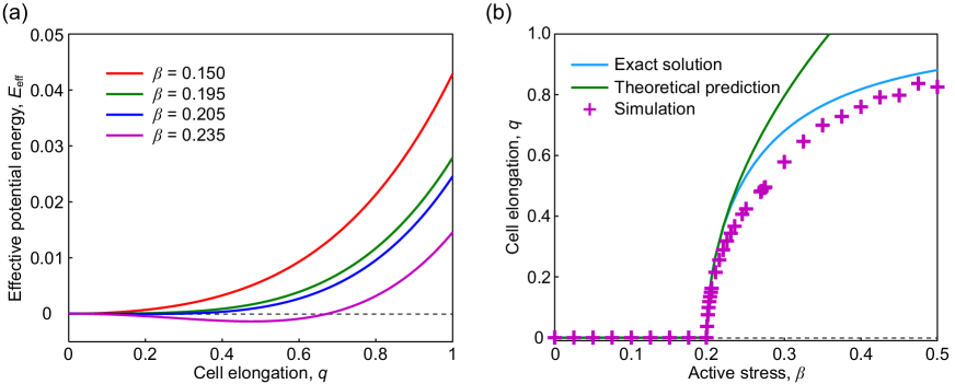
FIG. S9: Theoretical prediction of the cell elongation parameter $q$. (a) The effective potential energy Eq. (S32) as a function of the cell elongation parameter $q$ for different $\beta$ values. (b) Comparison of the elongation parameter $q$ of a hexagonal cell versus the cell activity $\beta$ between the exact solutions given by solving Eqs. (S18) and (S19), the theoretical predictions given by Eq. (S33), and numerical simulations of a single cell system. Parameters: $\tilde{K}_{P}=0.02$ and $\tilde{P}_{0}=1$, which results in $\tilde{\beta}_{1}\approx 0.1987$.

II.3 Simulations of single-cell system and four cell system

To gain physical insight into the tissue fluidization driven by cell-shape-controlled active stress, we also perform simulations in a single-cell system (Fig. S7) and a four-cell system (see main text Fig. 1(a), $\beta=0.150$). In both systems, initial configurations are regular hexagonal patterns with small perturbations applied to each vertex.

We find that both the single-cell system and the four-cell system exhibit an elongation transition at around $\beta\approx 0.20$ for $P_{0}=1$ (Fig. S10(a,c)), as in larger scale simulations (main text Fig. 1(c)). These two systems also undergo a second transition where some edges vanish. Specifically, the four-cell system undergo such a transition at $\beta\approx 0.25$ (Fig. S10(c)), which corresponds to the end of the solid anisotropic cell regime identified in our larger scale simulations (see also Movie S4 and S5 to visualize these transitions upon increasing $\beta$).

Further, we measure the minimum cell angle $\theta_{M}$ in the single-cell system. Interestingly, we find that the single cell system exhibits a perfect rhombile shape with the minimum cell angle $\theta_{M}\approx 60^{o}$ at $\beta\approx 0.3$. This can explain why we observe the maximum fraction of rhombile regime near $\beta\approx 0.30$.

In addition, we find that at the higher activity $\beta=0.4$, there are many metastable states in the four-cell system (Fig. S10(d)).

Finally, we compare the cell elongation parameter $q$ for simulations of the system-cell system, the four-cell system and the cell sheet system in Fig. S10(e); all agree very well for $\beta$ close to the first transition point.

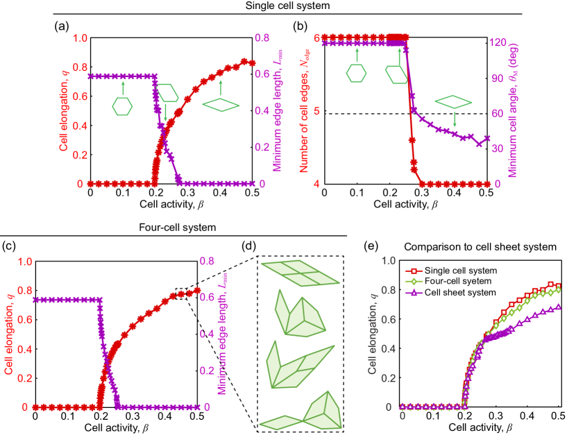
FIG. S10: Morphology transition driven by the active stress in (a,b) the single cell system, (c,d) the four-cell system, and (e) the cell sheet system. (a) The cell elongation parameter $q$ and the minimum edge length $L_{\rm min}$ versus the cell activity $\beta$. (b) The number of cell edges $N_{\rm edge}$ and the minimum cell angle $\theta_{\rm M}$ versus the cell activity $\beta$. (c) The cell elongation parameter $q$ and the minimum edge length $L_{\rm min}$ versus the cell activity $\beta$. (d) There exists multiple equilibrium states in the rhombile regime. Shown here are four typical equilibrium states for $\beta=0.45$. (e) Comparison of the cell elongation parameter $q$ in the single cell system, the four-cell system, and the cell sheet system. Parameters: $K_{P}=0.02$, $P_{0}=1$.

III Stability of the rhombile regime

III.1 The rhombile regime exhibits a finite shear modulus

We examine more closely the rheological properties of the rhombile regime defined in the main text. In Fig. S11(a), we represent a typical evolution curve of the shear stress before and after the application of a small simple shear deformation for $\beta=0.3$ ($P_{0}=1$). The sustained increase in the measured shear modulus is consistent with the interpretation that this tissue displays a finite shear modulus. We further perform a statistics in the measured shear modulus for different initial tissue configurations, see Sec. I.1; we find that the mean shear modulus is positive, Fig. S11(b), which is also consistent with the interpretation that the tissue displays, on average, a finite shear modulus. To confirm that such finite shear modulus is not due to numerical effects, we further investigated the roles of

• the T1 transition length threshold $\Delta_{\rm T1}$. We performed simulations with varied T1 transition length threshold $\Delta_{\rm T1}$ and we find that the shear modulus is not sensitive to $\Delta_{\rm T1}$; specifically for $\beta=0.3$, setting $\Delta_{\rm T1}=10^{-3},\ 10^{-2},\ 10^{-1}$ yielded consistent shear modulus values $G_{xy}/K_{P}=0.3244,\ 0.3000,\ 0.3321$, respectively.

• the amplitude of the simple shear strain $\gamma_{xy}$. We performed simulations varying $\gamma_{xy}$ and find that the shear modulus is not sensitive to $\gamma_{xy}$ in a broad range $10^{-5}-10^{-2}$. Specifically, for $\beta=0.3$, we measure that $G_{xy}=0.0069\pm 0.0046$ for $\gamma_{xy}=10^{-2}$, $G_{xy}=0.0068\pm 0.0046$ for $\gamma_{xy}=10^{-3}$, $G_{xy}=0.0069\pm 0.0047$ for $\gamma_{xy}=10^{-4}$, $G_{xy}=0.0071\pm 0.0047$ for $\gamma_{xy}=10^{-5}$.

We conclude that the tissue is solid within the identified rhombile regime.

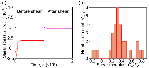
FIG. S11: The rhombile regime exhibits a finite shear modulus. (a) Evolution of the shear stress $\sigma_{xy}$ before and after the application of a small simple shear strain $\gamma_{xy}=0.01$. Shown here is a typical plot from $n=30$ independent simulations (initial hexagonal pattern with small perturbations). (b) Distribution of the measured shear modulus $G_{xy}$. $n=30$ independent simulations (initial hexagonal pattern with small perturbations) were performed.

III.2 Rhombile regime in systems of different sizes

To explore the effect of system size on the active stress driven tissue fluidity transition in cell sheets, here we vary the system size from a small one ($N=100$) to a large one ($N=10,000$). We find similar tissue fluidity transition regimes: as the cell activity $\beta$ is increased from small values to large values, the tissue transitions from the solid regime (isotropic cells), the solid regime (anisotropic cells), the rhombile regime, to finally the fluid regime, as shown in Fig. S12(a,b). Moreover, the critical $\beta$ values between these regimes for a large system ($N=10,000$) reads: $\beta_{1}\approx 0.20$, $\beta_{2}\approx 0.24$, and $\beta_{3}\approx 0.37$. These critical $\beta$ values are close to those presented in the main text. Finally, we present the rhombile regime in a large system ($N=10,000$) in Fig. S12(c).

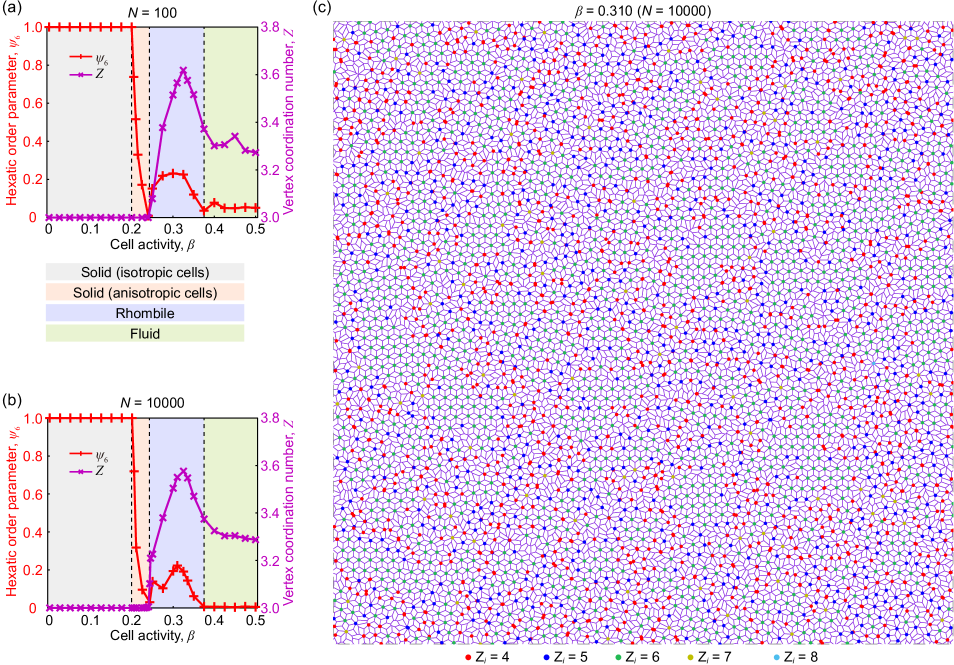
FIG. S12: Active-stress driven tissue fluidity transition in cell sheets of different sizes. (a, b) The hexatic order parameter $\psi_{6}$ and average vertex coordination number $Z$ versus cell activity $\beta$: (a) $N=100$; (b) $N=10,000$. (c) The rhombile regime ($\beta=0.31$) in a large cell sheet system ($N=10,000$). Parameters: $K_{P}=0.02$, and $P_{0}=1.0$.

III.3 Stability of a perfect rhombile pattern

Here we examine the stability of a global rhombile tiling pattern, as shown in Fig. S13(a), where cells are of identical diamond shape and display both 3-way and 6-way vertices. Here, the 6-fold vertices, being considered as a single vertex, cannot split into two separate 3-way vertices.

Our simulations show that the rhombile tiling pattern becomes unstable as the activity parameter $\beta$ is increased beyond the threshold value $\beta_{\rm cr,3}\approx 0.38$, see Fig. S13(a,b). The value $\beta_{\rm cr,3}\approx 0.38$ matches the value mentioned in the main text as delineating the rhombile regime from the disordered fluid regime.

We further estimated the shear modulus of the rhombile tiling pattern through numerical simulation, see Fig. S13(c) and find that the rhombile tiling pattern is of finite shear modulus for $\beta<\beta_{\rm cr,3}$. The presence of nucleated rhombile crystals may explain why a residual shear modulus can be observed within the rhombile regime.

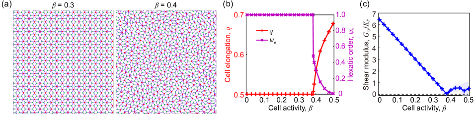
FIG. S13: Stability of the rhombile tiling pattern. Simulations are started from a rhombile tiling with small perturbations $\sigma=0.01$ in the position of each vertex. (a) Morphology of a cell sheet at different $\beta$ values. (b) The cell elongation $q$ and hexatic order $\psi_{6}$ versus cell activity $\beta$. (c) The long-time shear modulus $G_{xy}$ versus cell activity $\beta$. Parameters: $K_{P}=0.02$ and $P_{0}=1.0$.

IV Alternative cell shape descriptor

IV.1 Vertex-based inertia tensor

Definition

Here we first consider an alternative cell shape description to $\bm{Q}$ defined in terms of a vertex-based inertia tensor

$$\bm{M}_{v}=\sum_{i}{{{\bm{\rho}}_{i}}\otimes{{\bm{\rho}}_{i}}},$$ (S34)

where we have introduced the relative vertex position vectors $\bm{\rho}_{i}=\bm{r}_{i}-\bm{r}_{\rm C}$ with respect to the cell center $\bm{r}_{\rm C}=\sum_{k}\bm{r}_{k}/N$. By analogy to $\bm{Q}$ defined in main text, which is a deviatoric tensor, we define the following vertex-based inertia $\bm{Q}$-tensor:

$$\bm{Q}_{\rm inertia}=\frac{1}{2}\left[\frac{1}{\text{tr}\left(\bm{M}_{v}\right)}\bm{M}_{v}-\frac{1}{2}\bm{I}\right].$$ (S35)

FIG. S14: Solid-to-fluid transition driven by the active stress $\bm{\sigma}^{\rm(act)}=-\beta\bm{Q}_{\rm inertia}$, where $\bm{Q}_{\rm inertia}$ is defined by Eq. (S35). (a) Morphology of a cell sheet at different cell activities; we mark vertices with coordination number larger than 3, see Sec. I.4.1. (b) The cell elongation parameter $q$ and the T1 transition rate $k_{\rm T1}$ versus the cell activity $\beta$. (c) The hexatic order parameter $\psi_{6}$ and the average vertex coordination number $Z$ versus the cell activity $\beta$. (d) The (long-time) shear modulus $G_{xy}$ and the yield shear stress $\sigma_{\rm yield}$ versus the cell activity $\beta$. Parameters: $K_{P}=0.02$ and $P_{0}=1.0$.

Results

We find that the hexagonal pattern is destabilized at a critical coupling value $\beta_{c}\approx 0.2$, see Fig. S14(a,b) in favor of a solid regime with anisotropic cells in the range $\beta\in(0.2,0.35)$. Within the latter range of activity, we observe buckling along tissue-scale stripes, reminiscent of the chevron pattern within smectic A liquid crystal Limat and Prost (1993). Such chevron pattern is of finite shear modulus, Fig. S14(d). At a second critical value $\beta_{c}\approx 0.35$, the vertex coordinate number $Z$ increases, see Fig. S14(c), which marks the end of the solid regime with anisotropic cells. A rhombile crystal domains, with characteristic high proportion of periodically arranged six-fold vertices, are observed within an intermediate range of the coupling value $\beta$; here $\beta\in(0.35,0.58)$; in the latter range, both the vertex coordinate number $Z$ and hexatic order display a peak. For larger value of the coupling $\beta>0.58$, spontaneous flows take place.

Discussion

Overall, the results for the vertex-based inertia cell shape tensor are similar to the one presented in the main text. Following Ref. Nestor-Bergmann et al. (2018), one can show that the inertia tensor $\bm{M}_{v}$ displays the same principal orientations as the cell nematic shape tensor $\bm{Q}$ defined in the main text; yet the associated eigenvalues for these two tensors are, in general, different.

IV.2 Area-based inertia tensor

Definition

We next consider an area-based inertia tensor $\bm{M}_{a}$, defined as,

$$\bm{M}_{a}=\int{\left({{\left|\bm{r}\right|}^{2}}\bm{I}-\bm{r}\otimes\bm{r}\right){{\text{d}}^{2}}\bm{r}},$$ (S36)

where $\bm{r}$ is the position vector relative to the cell centroid. Similarly, we define the following $\bm{Q}$-tensor:

$$\bm{Q}_{\rm inertia}=\frac{5}{8}\left[\frac{1}{2}\bm{I}-\frac{1}{\text{tr}\left(\bm{M}_{a}\right)}\bm{M}_{a}\right].$$ (S37)

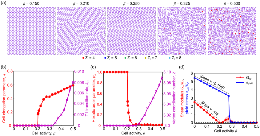
FIG. S15: Solid-to-fluid transition driven by the active stress $\bm{\sigma}^{\rm(act)}=-\beta\bm{Q}_{\rm inertia}$, where $\bm{Q}_{\rm inertia}$ is defined by Eq. (S37). (a) Morphology of a cell sheet at different cell activities; we mark vertices with a coordination number larger than 3. (b) The cell elongation parameter $q$ and the T1 transition rate $k_{\rm T1}$ versus the cell activity $\beta$. (c) The hexatic order parameter $\psi_{6}$ and the average vertex coordination number $Z$ versus the cell activity $\beta$. Parameters: $K_{P}=0.02$ and $P_{0}=1.0$.

Results - similarities with other schemes

We find that the hexagonal pattern is destabilized at a critical coupling value $\beta_{c}\approx 0.2$, see Fig. S15(a,b) in favor of a solid regime solid with anisotropic cells. Within the range $\beta\in(0.2,0.27)$, we also observe buckling along tissue-scale stripes (Fig. S15(a)) that are similar to those obtained with the vertex-based inertia tensor (Eq. (S35)); the corresponding tissue state display a finite shear modulus (Fig. S15(d)). At a second critical value $\beta_{2}\approx 0.27$, the vertex coordinate number $Z$ increases, see Fig. S15(c), which marks the end of the anisotropic solid regime. For larger value of the activity parameter $\beta>\beta_{3}=0.32$, spontaneous flows emerge.

Results - differences with other schemes

In the intermediate activity $(\beta_{2},\beta_{3})$, we observe some higher order vertices, but less than in the other schemes for $Q$. We do not observe well-defined rhombile crystal domains, Fig. S15(a,c).

Discussion

With the area-based inertia definition, the rhombile crystal pattern is not observed as $\beta$ is increased. We interpret that through a single cell shape analysis, which leads to less of shrinkage at cell edges in the case of the area-based inertia tensor. At the tissue level, this is reflected by a much smaller T1 transition rate $k_{\rm T1}$ (Fig. S15(b)) than for the standard inertia tensor $\bm{Q}$ defined on cell edges and Fig. 1(c)) or the vertex-based inertia tensor (Eq. (S35) and Fig. S14(b)).

V Cell shape texture and topological defects

V.1 Detection of topological defects

In presence of cell active stress, for $\beta>\beta_{1}$, a cell sheet exhibits elongated cell shape and coordinated orientations in local areas that are conflicting at singular points, called topological defects (see Fig. S16(a)).

To detect the locations and orientations of such topological defects, we first compute the cell geometric centers $\bm{r}_{J}=\sum_{i\in neighbor}\bm{r}_{i}/N_{J}$ with $N_{J}$ being the number of vertices belonging to the $J$-th cell, and the nematic tensors $\bm{Q}_{J}$ of cells. Based on $\bm{r}_{J}$ and $\bm{Q}_{J}$, we next construct a coarse-grained nematic field $\bm{Q}(\bm{r})$ on a regular grid,

$$\bm{Q}\left(\bm{r}\right)=\frac{\sum\limits_{\left|\bm{r}-{{\bm{r}}_{J}}\right|<{{r}_{\text{cut-off}}}}{w\left(\bm{r}-{{\bm{r}}_{J}}\right)\bm{Q}_{J}}}{\sum\limits_{\left|\bm{r}-{{\bm{r}}_{J}}\right|<{{r}_{\text{cut-off}}}}{w\left(\bm{r}-{{\bm{r}}_{J}}\right)}},$$ (S38)

where $w(\bm{r}-\bm{r}_{J})$ is the weight function and $r_{\rm cut-off}=3\sigma$ is a cut-off length. Here we set the weight function as a Gaussian function,

$$w\left(\bm{r}-{{\bm{r}}_{J}}\right)=\dfrac{1}{\sqrt{2\text{ }\!\!\pi\!\!\text{ }}\sigma}\exp\left(-\dfrac{1}{2}\dfrac{{{\left|\bm{r}-{{\bm{r}}_{J}}\right|}^{2}}}{{{\sigma}^{2}}}\right),$$ (S39)

where we set the kernel size $\sigma$ at $\sigma=0.75$ cell length. We set the cut-off length at $r_{\rm cut-off}=3\sigma=2.25$ cell length.

After obtaining the coarse-grained nematic field $\bm{Q}(\bm{r})$, we detect the location of topological defects based on the calculation of winding number Saw et al. (2017); Kawaguchi et al. (2017). The orientation of topological defects is extracted following the method presented in Vromans and Giomi (2016); for a topological charge $k$ ($k=\pm 1/2$), the orientation is given by

$$\psi=\frac{k}{1-k}\arctan 2\left[\left\langle{\rm sgn}\left(k\right)\frac{\partial{{Q}_{xy}}}{\partial x}-\frac{\partial{{Q}_{xx}}}{\partial y}\right\rangle,\left\langle\frac{\partial{{Q}_{xx}}}{\partial x}+{\rm sgn}\left(k\right)\frac{\partial{{Q}_{xy}}}{\partial y}\right\rangle\right],$$ (S40)

where $\langle\cdot\rangle$ denotes an average along the shortest available loop enclosing the defect core; $\rm sgn(\cdot)$ is the sign function; $\arctan 2(y,x)$ is the 2-argument arctangent function.

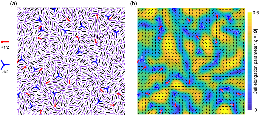
FIG. S16: Topological defect detection scheme. (a) The original cell sheet morphology superimposed with the detected topological defects (red and blue markers). The black lines indicate cell orientations, given by the cell shape nematic tensors $\bm{Q}_{J}$. (b) The coarse-grained nematic tensor field superimposed with the detected topological defects, where the color code refers to the cell elongation parameter $q=|\bm{Q}|$ and the black lines indicate local nematic orientations given by $\bm{Q}$.

To check the reliability of such detection scheme, we superimpose the detected topological defects on the original cell sheet morphology and coarse-grained nematic field, as shown in Fig. S16. We can see that the detected topological defects fit well with both the original cell sheet morphology and the coarse-grained nematic field. We mainly observe two kinds of topological defects, i.e., comet-like $+1/2$ topological defects and trefoil-like $-1/2$ topological defects.

V.2 Stress and flow fields near topological defects

We examine the average stress and flow fields near $\pm 1/2$ topological defects in our vertex model implementation. The resulting fields are consistent with the predictions of an incompressible active nematic continuum theory Saw et al. (2017). Method – We first examine the average isotropic stress ($\sigma_{\rm iso}=(\sigma_{xx}+\sigma_{yy})/2$) field. We first define a local coordinate system of a topological defect: its origin locates at the defect core, with $x$-axis along the defect orientation. The average isotropic stress $\hat{\sigma}_{\text{iso}}$ at position $\bm{x}$ (local coordinate system) is estimated through the following expression

$${\hat{\sigma}_{\text{iso}}}\left(\bm{x}\right)=\frac{\sum\limits_{\left|\bm{x}-{{{\bm{\bar{r}}}}_{J,\alpha}}\right|<{{r}_{\text{cut-off}}}}{w\left(\bm{x}-{{{\bm{\bar{r}}}}_{J,\alpha}}\right)\sigma_{\text{iso}}^{\left(J\right)}}}{\sum\limits_{\left|\bm{x}-{{{\bm{\bar{r}}}}_{J,\alpha}}\right|<{{r}_{\text{cut-off}}}}{w\left(\bm{x}-{{{\bm{\bar{r}}}}_{J,\alpha}}\right)}}.$$ (S41)

Here $\sigma_{\rm iso}^{(J)}$ is the isotropic stress of the $J$-th cell; $w(\cdot)$ is a Gaussian weight function (Eq. (S39)); $\bar{\bm{r}}_{J,\alpha}$ represents the position vector of the geometric centre of the $J$-th cell relative to the $\alpha$-th topological defect, and can be calculated according to the following expression:

$${{\bm{\bar{r}}}_{J,\alpha}}=\mathcal{R}\left[\left({{\bm{r}}_{J}}-{{\bm{x}}_{\alpha}}\right);-{{\theta}_{\alpha}}\right],$$ (S42)

where $\theta_{\alpha}$ refers to the orientation of the $\alpha$-th topological defect; $\mathcal{R}[\bm{r};\theta]$ represents a rotation of the vector $\bm{r}$ by an angle $\theta$. Similarly, the average flow velocity $\hat{\bm{v}}(\bm{x})$ at position $\bm{x}$ (local coordinate system) is estimated as

$$\bm{\hat{v}}\left(\bm{x}\right)=\frac{\sum\limits_{\left|\bm{x}-{{{\bm{\bar{r}}}}_{J,\alpha}}\right|<{{r}_{\text{cut-off}}}}{\omega\left(\bm{x}-{{{\bm{\bar{r}}}}_{J,\alpha}}\right)\mathcal{R}\left[{{\bm{v}}_{J}};-{{\theta}_{\alpha}}\right]}}{\sum\limits_{\left|\bm{x}-{{{\bm{\bar{r}}}}_{J,\alpha}}\right|<{{r}_{\text{cut-off}}}}{\omega\left(\bm{x}-{{{\bm{\bar{r}}}}_{J,\alpha}}\right)}},$$ (S43)

where $\bm{v}_{J}=\mathrm{d}\bm{r}_{J}/\mathrm{d}t$ is the motion velocity of the $J$-th cell.

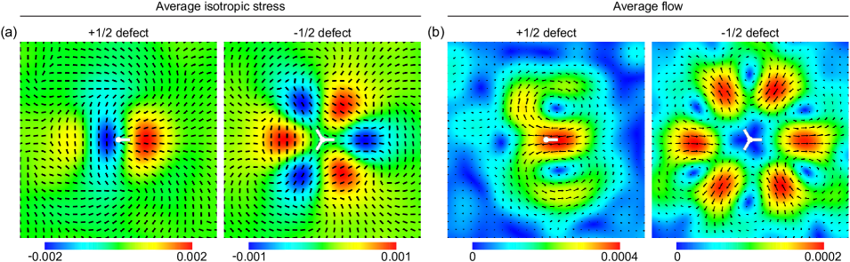
FIG. S17: The isotropic stress field (a) and flow field (b) near half-integer topological defects, averaged over thousands of topological defects ($n_{\pm 1/2}=9,844$). In (a), the color code refers to the local stress fluctuation $\sigma_{\rm iso}-\langle\sigma_{\rm iso}\rangle$ and the black lines indicate local cell orientations. In (b), the color code refers to the velocity magnitude $|\bm{v}|$ and black arrows indicate local flow velocity vectors. Domain size: $L=10$. Parameters: $K_{P}=0.02$, $P_{0}=1$, and $\beta=0.4$.

Result – Figure S17 shows the coarse-grained average isotropic stress and flow fields near $\pm 1/2$ topological defects, for $\beta=0.4>0$ (extensile active nematic case). We observe that both the stress and flow fields are consistent with previous experimental measurements (including MDCK cell monolayer system Saw et al. (2017); Balasubramaniam et al. (2021), human bronchial epithelial cell monolayer system Blanch-Mercader et al. (2018) and neural progenitor cell monolayer system Kawaguchi et al. (2017)) and predictions of a continuum active gel theory Giomi (2015); Saw et al. (2017).

V.3 Cell-cell rearrangement field near topological defects

In the main text Figure 3, we examine the cell-cell rearrangement rate field near topological defects. We define the cell rearrangement rate as the number of T1 transitions per unit time per unit area, estimated according to the following formula

$$\chi\left(\bm{x}\right)=\frac{\sum\limits_{\left|\bm{x}-{{{\bm{\bar{r}}}}_{T,\alpha}}\right|<{{r}_{\text{cut-off}}}}{\delta\left(\bm{x}-{{{\bm{\bar{r}}}}_{T,\alpha}}\right)}}{\text{ }\!\!\pi\!\!\text{ }r_{\text{cut-off}}^{2}\tau},$$ (S44)

where ${{\bm{\bar{r}}}_{T,\alpha}}=\mathcal{R}\left[\left({{\bm{r}}_{T}}-{{\bm{x}}_{\alpha}}\right);-{{\theta}_{\alpha}}\right]$ represents the position vector of the $T$-th T1 transition relative to the $\alpha$-th topological defect; the observation period spans a duration $\tau$ preceeding the end of simulation (here $\tau=200$).

VI Thresholdless flows

For $P_{0}>P_{0}^{\ast}\approx 3.72$ (hexagonal cell pattern), we observe spontaneous tissue flows for very small cell activity, suggesting that the transition to flow is thresholdless, i.e. at exactly $\beta=0$ in the limit of a very large system $N\rightarrow\infty$.

For illustration, here we set $P_{0}=4.2$ and vary $\beta$. Figure S18(a) shows the morphology of a cell sheet at zero cell activity ($\beta=0$) and small cell activity ($\beta=0.001$), respectively. We observe strikingly different cell morphologies at $\beta=0$ and $\beta=0.001$: in the former, cells are concave polygons, with no rosettes; in the latter, cells are elongated $\beta=0.001$, with many involved in rosettes. In Fig. S18(b) we represent the T1 transition rate $k_{\rm T1}$ as a function of cell activity $\beta$ for different system sizes. Notably, when the system size is increased, the activity threshold for spontaneous T1 transitions shifts towards zero, which suggests thresholdless tissue flows. In addition, we observe a discontinuous (first-order like) transition at $\beta=0$ in both the cell elongation parameter $q$ and the average vertex coordination number $Z$ upon increasing cell activity $\beta$, as shown in Fig. S18(c). These results suggest that even a very small cell activity leads to a drastic change in the cell shape pattern (including the onset of multicellular rosettes).

FIG. S18: Thresholdless tissue flows for $P_{0}>P_{0}^{\ast}$. (a) Tissue configuration at $\beta=0$ (left) and $\beta=0.001$ (right). (b) The T1 transition rate $k_{\rm T1}$ versus cell activity $\beta$ for different system sizes ($N=100,\ 400,\ 1000$). (c) The cell elongation parameter $q$ and the average vertex coordination number $Z$ versus cell activity $\beta$. Here, system size $N=1000$. Parameters: $K_{P}=0.02$ and $P_{0}=4.2$.

VII Supplemental Movies

Movie S1. Activity-induced melting Tissue evolution under a gradually increasing cell activity, from $\beta=0.17$ to $\beta=0.50$. Here, we progressively increase the cell activity $\beta$ according to the step-by-step increase procedure: $\beta^{(n+1)}=\beta^{(n)}+\Delta\beta$, with $\Delta\beta=0.003$; after each step increase in the cell activity, we relax the system for a time $t_{\rm relax}=1,000$ (in $\gamma/K_{A}A_{0}$ unit). Parameters: $K_{P}=0.02$ and $P_{0}=1$.

Movie S2. Hexagonal initial condition Tissue evolution at different cell active stress levels ($\beta=0.210,\ 0.325,\ 0.450$). Parameters: $K_{P}=0.02$ and $P_{0}=1$.

Movie S3. Voronoi initial condition Tissue evolution at different cell active stress ($\beta=0.210,\ 0.325,\ 0.450$) levels for cells initially arranged according to a Voronoi pattern. Parameters: $K_{P}=0.02$ and $P_{0}=1$.

Movie S4. Four-cell system with free boundary Evolution of a four-cell tissue under a gradually increasing cell activity, from $\beta=0.1$ to $\beta=0.5$. Here, we increase the cell activity $\beta$ step-by-step, $\beta^{(n+1)}=\beta^{(n)}+\Delta\beta$ with $\Delta\beta=0.004$; after each increase in the cell activity, we relax the system for a time $t_{\rm relax}=20,000$ (in $\gamma/K_{A}A_{0}$ unit). Parameters: $K_{P}=0.02$ and $P_{0}=1$.

Movie S5. Single-cell system with free boundary Evolution of a single-cell tissue under a gradually increasing cell activity, from $\beta=0.1$ to $\beta=0.5$. Here, we increase the cell activity $\beta$ step-by-step, $\beta^{(n+1)}=\beta^{(n)}+\Delta\beta$ with $\Delta\beta=0.004$; after each increase in the cell activity, we relax the system for a time $t_{\rm relax}=20,000$ (in $\gamma/K_{A}A_{0}$ unit). Parameters: $K_{P}=0.02$ and $P_{0}=1$.

Movie S6. Four-cell system with periodic boundary Periodic oscillations in a four-cell system under periodic boundary conditions. Parameters: $K_{P}=0.02$, $P_{0}=1$, and $\beta=0.315$.

Movie S7. Vertex-based inertia tensor Tissue time evolution for different cell active stress levels using the vertex-based inertia tensor ($\beta=0.250,\ 0.450,\ 0.800$). Parameters: $K_{P}=0.02$ and $P_{0}=1$.

Movie S8. Area-based inertia tensor Tissue time evolution for different cell active stress levels using the area-based inertia tensor ($\beta=0.210,\ 0.250,\ 0.325$). Parameters: $K_{P}=0.02$ and $P_{0}=1$.

References

- Fletcher et al. (2014) A. G. Fletcher, M. Osterfield, R. E. Baker, and S. Y. Shvartsman, Biophysical Journal 106, 2291–2304 (2014).
- Bi et al. (2015) D. Bi, J. H. Lopez, J. M. Schwarz, and M. L. Manning, Nature Physics 11, 1074 (2015).
- Lin et al. (2018) S. Z. Lin, S. Ye, G. K. Xu, B. Li, and X. Q. Feng, Biophysical Journal 115, 1826–1835 (2018).
- Batchelor (1970) G. K. Batchelor, Journal of Fluid Mechanics 41, 545 (1970).
- Lau and Lubensky (2009) A. W. C. Lau and T. C. Lubensky, Physical Review E 80, 011917 (2009).
- Nestor-Bergmann et al. (2018) A. Nestor-Bergmann, G. Goddard, S. Woolner, and O. E. Jensen, Mathematical Medicine and Biology 35, 1 (2018).
- Merkel et al. (2019) M. Merkel, K. Baumgarten, B. P. Tighe, and M. L. Manning, Proceedings of the National Academy of Sciences of the United States of America 116, 6560 (2019).
- Li and Ciamarra (2018) Y. W. Li and M. P. Ciamarra, Physical Review Materials 2, 45602 (2018).
- Paoluzzi et al. (2021) M. Paoluzzi, L. Angelani, G. Gosti, M. C. Marchetti, I. Pagonabarraga, and G. Ruocco, Physical Review E 104, 044606 (2021).
- Farhadifar et al. (2007) R. Farhadifar, J. C. Röper, B. Aigouy, S. Eaton, and F. Jülicher, Current Biology 17, 2095 (2007).
- Sussman and Merkel (2018) D. M. Sussman and M. Merkel, Soft Matter 14, 3397 (2018).
- Wang et al. (2020) X. Wang, M. Merkel, L. B. Sutter, G. Erdemci-Tandogan, M. L. Manning, and K. E. Kasza, Proceedings of the National Academy of Sciences of the United States of America 117, 13541 (2020).
- Limat and Prost (1993) L. Limat and J. Prost, Liquid Crystals 13, 101 (1993).
- Saw et al. (2017) T. B. Saw, A. Doostmohammadi, V. Nier, L. Kocgozlu, S. Thampi, Y. Toyama, P. Marcq, C. T. Lim, J. M. Yeomans, and B. Ladoux, Nature 544, 212 (2017).
- Kawaguchi et al. (2017) K. Kawaguchi, R. Kageyama, and M. Sano, Nature 545, 327 (2017).
- Vromans and Giomi (2016) A. J. Vromans and L. Giomi, Soft Matter 12, 6490 (2016).
- Balasubramaniam et al. (2021) L. Balasubramaniam, A. Doostmohammadi, T. B. Saw, G. H. N. S. Narayana, R. Mueller, T. Dang, M. Thomas, S. Gupta, S. Sonam, A. S. Yap, et al., Nature Materials 20, 1156 (2021).
- Blanch-Mercader et al. (2018) C. Blanch-Mercader, V. Yashunsky, S. Garcia, G. Duclos, L. Giomi, and P. Silberzan, Physical Review Letters 120, 208101 (2018).
- Giomi (2015) L. Giomi, Physical Review X 5, 031003 (2015).
- Mueller et al. (2019) R. Mueller, J. M. Yeomans, and A. Doostmohammadi, Physical Review Letters 122, 48004 (2019).