MPC-Based Emergency Vehicle-Centered Multi-Intersection Traffic Control

Abstract

This paper proposes a traffic control scheme to alleviate traffic congestion in a network of interconnected signaled lanes/roads. The proposed scheme is emergency vehicle-centered, meaning that it provides an efficient and timely routing for emergency vehicles. In the proposed scheme, model predictive control is utilized to control inlet traffic flows by means of network gates, as well as configuration of traffic lights across the network. Two schemes are considered in this paper: i) centralized; and ii) decentralized. In the centralized scheme, a central unit controls the entire network. This scheme provides the optimal solution, even though it might not fulfil real-time computation requirements for large networks. In the decentralized scheme, each intersection has its own control unit, which sends local information to an aggregator. The main responsibility of this aggregator is to receive local information from all control units across the network as well as the emergency vehicle, to augment the received information, and to share it with the control units. Since the decision-making in decentralized scheme is local and the aggregator should fulfil the above-mentioned tasks during a traffic cycle which takes a long period of time, the decentralized scheme is suitable for large networks, even though it may provide a sub-optimal solution. Extensive simulation studies are carried out to validate the proposed schemes, and assess their performance. Notably, the obtained results reveal that traveling times of emergency vehicles can be reduced up to $\sim$50% by using the centralized scheme and up to $\sim$30% by using the decentralized scheme, without causing congestion in other lanes.

I Introduction

Traffic congestion is one of the most critical issues in urbanization. In particular, many cities around the world have experienced 46–70% increase in traffic congestion [1]. Congested roads not only lead to increased commute times, but also hinder timely deployment of emergency vehicles [2]. Hence, emergency vehicles often fail to meet their target response time [3]. According to $\sim$240 million emergency calls every year in the U.S. [4], such hindering greatly affects hospitalization and mortality rates [5].

The common practice by regular vehicles (i.e., non-emergency vehicles) in the presence of an emergency vehicle is to pull over to the right (in two-way roads) or to the nearest shoulder (in one-way roads) [6], and let the emergency vehicle traverse efficiently and timely. This is not always possible, as in dense areas the edges of the roads are usually occupied by parked/moving vehicles.

The chance of an emergency vehicle getting stuck is even higher when it has to traverse intersections with cross-traffic [7]. Note that the majority of incidents involving emergency vehicles happen within intersections [8]. One possible way to cope with this problem is to use traffic lights at intersections to detect emergency vehicles and facilitate their fast and efficient travel. For this purpose, traffic lights in most parts of the U.S. are equipped with proper detectors (e.g., 3M Opticom^™ [9]), and emergency vehicles are equipped with emitters which broadcast an infrared signal. When the receiver on a traffic light detects a recognized signal, the traffic light changes to allow priority access to the emergency vehicle. In this context, the “green wave” method has been proposed to reduce emergency vehicles’ traveling time [10]. In the “green wave” method, a series of traffic lights are successively set to ‘green’ to allow timely passage of emergency vehicles through several intersections [11]. The main issue with the “green wave” method is that it leads to prolonged red lights for other lanes [12], meaning that it may cause congestion in other lanes.

A different method for controlling the traffic in the presence of an emergency vehicle is to convert the traffic control problem to a real-time scheduling problem [13, 3]. The core idea of this method is to model the vehicles and traffic lights as aperiodic tasks and sporadic servers, respectively, and then to utilize available task scheduling schemes to solve the resulting problem. Other existing traffic control methods either do not consider emergency vehicles [14, 15, 16, 17, 18, 19] or require vehicle to vehicle connectivity [20, 21, 22, 23, 24, 25]. Note that the presence of 100% of connected vehicles is not expected until 2050 [26], making these methods inapplicable to the current traffic systems.

The aim of this paper is to propose control algorithms to manipulate traffic density in a network of interconnected signaled lanes. The core idea is to integrate the Cell Transmission Model (CTM) [27, 28] with Model Predictive Control (MPC) [29]. Our motivation to use MPC is that it solves an optimal control problem over a receding time window, which provides the capability of predicting future events and taking actions accordingly. Note that even though this approach is only sub-optimal, in general [30], it works very well in many applications; our numerical experiments suggest that MPC yields very good performance in traffic control applications. Two schemes are developed in this paper: i) centralized; and ii) decentralized. In the centralized scheme, assuming that the control inputs are inlet traffic flows and configuration of the traffic lights across the network, a two-step control scheme is proposed. In a normal traffic mode, the proposed centralized scheme alleviates traffic density in all lanes, ensuring that traffic density in the entire network is less than a certain value. When an emergency vehicle approaches the network—this condition is referred as an emergency traffic mode—the control objective is to clear the path for the emergency vehicle, without causing congestion in other lanes. It is shown that our proposed centralized scheme provides the optimal solution, even though its computation time may be large for large networks. In the decentralized scheme, inlet traffic flows and configuration of the traffic lights at each intersection are controlled by a local control unit, while the control units share data with each other through an aggregator. In the decentralized scheme, the aggregator should receive and send the data during every traffic light state (i.e., ‘red’ or ‘green’). Since the traffic cycle ranges from one minute to three minutes in real-world traffic systems [31], the smallest duration of traffic light states is 30 seconds; thus, the maximum allowable communication delay is around 30 seconds, which is achievable even with cheap communication technologies. Thus, the decentralized scheme is more suitable for large networks, even though it yields a sub-optimal solution. Note that the robustness and tolerance of the decentralized scheme to uncertainty in communication delay and communication failures are out of the scope of this paper, and will be considered as future work.

The key contributions of this paper are: i) we develop a traffic control framework which provides an efficient and timely emergency vehicle passage through multiple intersections, without causing congestion in other lanes; ii) we propose a centralized scheme for small networks and a decentralized scheme for large networks that addresses scalability issues in integrating CTM and MPC; and iii) we validate our schemes via extensive simulation studies, and assess their performance in different scenarios. The main features of the proposed framework are: i) it is general and can be applied to any network of interconnected signaled lanes; and ii) it does not require vehicle to everything (V2X) connectivity, and hence it can be utilized in the currently existing traffic systems; the only communication requirement is between the emergency vehicle and the central control unit in the centralized scheme, and with the aggregator in the decentralized scheme. Note that this paper considers only macroscopic characteristics of traffic flow; it is evident that the existence of V2X connectivity can not only be exploited to further improve efficiency at the macro-level, but it can also be leveraged to ensure safety and avoid collisions.

The key innovations of this paper with respect to prior work are: i) formulating the traffic density control problem in both normal and emergency modes as MPC problems; ii) developing a two-step optimization procedure implementable in the current traffic systems; and iii) deriving centralized and decentralized schemes for traffic networks with different size and communication capacity.

The rest of the paper is organized as follows. Section II describes macroscopic discrete-time model of the traffic flow in the network. Section III discusses the design procedure of the centralized traffic control scheme. The decentralized scheme is discussed in Section IV. Section V reports simulations results and compares the centralized and decentralized schemes. Finally, Section VI concludes the paper.

Notation

$\mathbb{R}$ denotes the set of real numbers, $\mathbb{R}_{\geq 0}$ denotes the set of non-negative real numbers, $\mathbb{Z}$ denotes the set of integer numbers, and $\mathbb{Z}_{\geq 0}$ denotes the set of non-negative integer numbers. For the matrix $X$, $X^{\top}$ denotes its transpose, $\rho(X)$ denotes its spectral radius, and $\left\|X\right\|_{1}=\sup_{y\neq 0}\frac{\left\|Xy\right\|_{1}}{\left\|y\right\|_{1}}$ with $\left\|\cdot\right\|_{1}$ as the $\ell_{1}$-norm. For the vector $y$, $[y]_{+}$ is the element-wise rounding to the closest non-negative integer function. For given sets $X,Y$, $X\oplus Y:\{x+y:x\in X,y\in Y\}$ is the Minkowski set sum. TABLE I lists the essential notation of this paper.

TABLE I: List of calligraphic, Greek, Latin, and subscript and superscript symbols.

Type	Symbol	Description
Calligraphic	$\mathcal{N}$	Set of lanes
	$\mathcal{M}$	Set of intersections
	$\mathcal{G}$	Traffic network
	$\mathcal{E}$	Edge of traffic graph
	$\mathcal{X}$	Constraint set
	$\mathcal{D}$	Disturbance set
Greek	$\Lambda$	Set of possible commands by traffic lights
	$\lambda$	Configuration of traffic lights
	$\gamma$	Prioritizing parameter
Latin	$x$	Traffic density
	$y$	Traffic inflow
	$z$	Traffic outflow
	$u$	Inlet flow
	$d$	Disturbance input
	$t$	Discrete time instant
	$k$	Prediction time instant
Subscript and	$in$	inlet
Superscript	$df$	Disturbance-free
	$nom$	Nominal
	$n$	normal condition
	$e$	Emergency condition
	$t$	Computed at time $t$

II System Modelling

In this section, we formulate the traffic control problem for a general traffic network.

II-A Traffic Network

Consider a traffic network with $N$ lanes and $M$ intersections. There are $N_{in}<N$ inlets through which vehicles enter the network. We denote the set of lanes by $\mathcal{N}=\{1,\cdots,N\}$, the set of intersections by $\mathcal{M}=\{1,\cdots,M\}$, and the set of inlets by $\mathcal{N}_{in}\subset\mathcal{N}$.

The considered traffic network can be represented by a graph $\mathcal{G}(\mathcal{N},\mathcal{E})$, where $\mathcal{E}\subset\mathcal{N}\times\mathcal{N}$ defines the edge of graph. The edge $(i,j)\in\mathcal{E}$ represents a directed connection from lane $i$ to lane $j$. Since all lanes are assumed to be unidirectional (note that two-way roads are modeled as two opposite-directional lanes), if $(i,j)\in\mathcal{E}$, we have $(j,i)\not\in\mathcal{E}$. Also, we assume that U-turns are not allowed, i.e., $(i,j),(j,i)\not\in\mathcal{E}$, if lanes $i$ and $j$ are opposite-directional lanes on a single road.

Note that we assume that the traffic graph $\mathcal{G}(\mathcal{N},\mathcal{E})$ remains unchanged; that is we do not consider graph changes due to unexpected events (e.g., changes in the edge $\mathcal{E}$ as a result of lane blockages due to accidents). We leave the developments of strategies for rerouting in the case of a change in the traffic graph to future work.

II-B Action Space By Traffic Lights

Suppose that all lanes, except outlets, are controlled by traffic lights which have three states: ‘red’, ‘yellow’, and ‘green’. The vehicles are allowed to move when the light is ‘yellow’ or ‘green’, while they have to stop when the light is ‘red’. This means that there are practically two states for each traffic light.

Let $\lambda_{j}(t)$ be the configuration of traffic lights at intersection $j\in\mathcal{M}$ at time $t$. We denote the set of all possible configurations at intersection $j$ by $\Lambda_{j}=\{\lambda_{j,1},\cdots,\lambda_{j,\mu_{j}}\}$, where $\mu_{j}\in\mathbb{Z}_{\geq 0}$. Indeed, the set $\Lambda_{j}$ represents the set of all possible actions that can be commanded by the traffic lights at intersection $j$. Therefore, the set of all possible actions by traffic lights across the network is $\Lambda=\Lambda_{1}\times\cdots\times\Lambda_{M}$, and the $M$-tuple $\lambda(t)=\big{(}\lambda_{1}(t),\cdots,\lambda_{M}(t)\big{)}\in\Lambda$ indicates the action across the network at time $t$.

II-C Macroscopic Traffic Flow Model

The traffic density in each lane is a macroscopic characteristic of traffic flow [32, 33], which can be described by the CTM that transforms the partial differential equations of the macroscopic Lighthill-Whitham-Richards (LWR) model [34] into simpler difference equations at the cell level. The CTM formulates the relationship between the key traffic flow parameters, and can be cast in a discrete-time state-space form.

Let traffic density be defined as the total number of vehicles in a lane at any time instant, then the traffic inflow is defined as the total number of vehicles entering a lane during a given time period, and traffic outflow is defined as the total number of vehicles leaving a lane during a given time period. We use $x_{i}(t)\in\mathbb{Z}_{\geq 0}$, $y_{i}(t)\in\mathbb{R}_{\geq 0}$, and $z_{i}(t)\in\mathbb{R}_{\geq 0}$ to denote the traffic density, traffic inflow, and traffic outflow in lane $i$ at time $t$, respectively. The traffic dynamics [35, 36] in lane $i$ can be expressed as

$$x_{i}(t+1)=\left[x_{i}(t)+y_{i}(t)-z_{i}(t)\right]_{+},$$ (1)

where the time interval $[t,t+1)$ is equivalent to $\Delta T$ seconds. Since $x_{i}(t)$ is defined as the number of existing vehicles in each lane, we use the rounding function in (1) to ensure that $x_{i}(t)$ remains a non-negative integer at all times. Given $\Delta T$, $y_{i}(t)$ and $z_{i}(t)$ are equal to the number of vehicles entering and leaving the lane $i$ in $\Delta T$ seconds, respectively.

The traffic outflow $z_{i}(t)$ can be computed as [19]

$$z_{i}(t)=p_{i}\big{(}\lambda(t)\big{)}x_{i}(t),$$ (2)

where $p_{i}\big{(}\lambda(t)\big{)}$ is the fraction of outflow vehicles in lane $i$ during the time interval $[t,t+1)$, satisfying

$$p_{i}\big{(}\lambda(t)\big{)}\left\{\begin{array}[]{ll}=0,&\text{if traffic light of lane }i\text{ is `red'}\\ \in[0,1],&\text{if traffic light of lane }i\text{ is `green'}\end{array}\right.;$$ (5)

in other words, $p_{i}\big{(}\lambda(t)\big{)}$ is the ratio of vehicles leaving lane $i$ during the time interval $[t,t+1)$ to the total number of vehicles in lane $i$ at time instant $t$. It is noteworthy that even though the impact of lane blockage or an accident in lane $i$ can be modeled by adjusting $p_{i}\big{(}\lambda(t)\big{)}$, this paper does not aim to deal with such unexpected events.

Remark II.1

We assume that outlet traffic flows are uncontrolled, i.e., there is no traffic light or gate at the end of outlets. This assumption is plausible, as any road connecting the considered traffic network to the rest of the grid can be divided at a macro-level into an uncontrollable outlet inside the considered network and a lane outside the considered network (possibly controlled with a traffic light or a network gate). The extension of the proposed methods to deal with controlled outlet flows is straightforward by modifying (2) and all presented optimization problems to account for outlet flow (similar to what we do for inlet flow $u_{i}(t)$); thus, to simplify the exposition and subsequent developments, we will not discuss controlled outlets.

The traffic inflow $y_{i}(t)$ can be computed as

$$y_{i}(t)=\left\{\begin{array}[]{ll}u_{i}(t),&\text{if $i\in\mathcal{N}_{in}$}\\ \sum\limits_{j=1}^{N}q_{j,i}\big{(}\lambda(t)\big{)}z_{j}(t),&\text{otherwise}\end{array}\right.,$$ (8)

where $u_{i}(t)\in\mathbb{Z}_{\geq 0}$ is the inlet flow which is defined as the number of vehicles entering the traffic network through inlet $i$ during the time interval $[t,t+1)$. The computed optimal inflows can be implemented by means of network gates, i.e., ramp meters [37, 38] for highways and metering gates [39] for urban streets). In (8), $q_{j,i}\big{(}\lambda(t)\big{)}$ is the fraction of outflow of lane $j$ directed toward lane $i$ during the time interval $[t,t+1)$, which is

$$q_{j,i}\big{(}\lambda(t)\big{)}\left\{\begin{array}[]{ll}=0,&\text{(if traffic light of lane $i$ is `red')}\\ &\text{OR (if }(j,i)\not\in\mathcal{E}\text{)}\\ \in[0,1],&\text{(if traffic light of lane $i$ is `green')}\\ &\text{AND (if }(j,i)\in\mathcal{E}\text{)}\end{array}\right.,$$ (13)

and satisfies $\sum_{i=1}^{N}q_{j,i}\big{(}\lambda(t)\big{)}=1$ for all $j\in\mathcal{N}$. More precisely, $q_{j,i}\big{(}\lambda(t)\big{)}$ is the ratio of vehicles leaving lane $j$ and entering lane $i$ during the time interval $[t,t+1)$ to the total number of vehicles leaving lane $j$ during the time interval $[t,t+1)$.

From (1)-(13), traffic dynamics of the entire network can be expressed as

$$x(t+1)=\left[\bar{A}\big{(}\lambda(t)\big{)}x(t)+B\bar{U}(t)\right]_{+},$$ (14)

where $x(t)=[x_{1}(t)~{}\cdots~{}x_{N}(t)]^{\top}\in\mathbb{Z}_{\geq 0}^{N}$, $\bar{A}:\Lambda\rightarrow\mathbb{R}^{N\times N}$ is the so-called traffic tendency matrix [40], $B\in\mathbb{R}^{N\times N_{in}}$, and $\bar{U}(t)\in\mathbb{Z}_{\geq 0}^{N_{in}}$ is the boundary inflow vector. It should be noted that the $(i,j)$ element of $B$ is 1 if lane $i$ is the $j$-th inlet, and 0 otherwise.

Remark II.2

At any $t$, the $(i,i)$ element of the traffic tendency matrix $\bar{A}\big{(}\lambda(t)\big{)}$ is $1-p_{i}\big{(}\lambda(t)\big{)}$. Also, its $(i,j)$ element ($i\neq j$) is $q_{j,i}\big{(}\lambda(t)\big{)}p_{j}\big{(}\lambda(t)\big{)}$. As a result, since $\sum_{i=1}^{N}q_{j,i}\big{(}\lambda(t)\big{)}=1,~{}\forall j\in\mathcal{N}$, the maximum absolute column sum of the traffic tendency matrix is less than or equal to 1. This means that at any $t$, we have $\left\|\bar{A}\big{(}\lambda(t)\big{)}\right\|_{1}\leq 1$, which implies that $\rho\Big{(}\bar{A}\big{(}\lambda(t)\big{)}\Big{)}\leq 1$. Therefore, $\rho\Big{(}\bar{A}\big{(}\lambda(t)\big{)}\bar{A}\big{(}\lambda(t+1)\big{)}\bar{A}\big{(}\lambda(t+2)\big{)}\cdots\Big{)}\leq 1$, which means that the unforced system (i.e., when $\bar{U}(t)=0$) is stable, although trajectories may not asymptotically converge to the origin. This conclusion is consistent with the observation that in the absence of new vehicles entering to lane $i$, the traffic density in lane $i$ remains unchanged if the corresponding traffic light remains ‘red’.

Remark II.3

In general, system (14) is not bounded-input-bounded-output stable. For instance, the traffic density in lane $i$ constantly increases if $y_{i}(t)>0$ at all times and the corresponding traffic light remains ‘red’.

Given the action $\lambda(t)$, the traffic dynamics given in (14) depend on the parameters $p_{i}\big{(}\lambda(t)\big{)}$ and $q_{j,i}\big{(}\lambda(t)\big{)},~{}\forall i,j$, as well as the boundary inflow vector $\bar{U}(t)$. These parameters are, in general, a priori unknown. We assume that these parameters belong to some bounded intervals, and we can estimate these intervals from prior traffic data. Thus, traffic dynamics given in (14) can be rewritten as

$$x(t+1)=\Big{[}\Big{(}A\big{(}\lambda(t)\big{)} +\Delta A(t)\Big{)}x(t)$$

$$+B\big{(}U(t)+\Delta U(t)\big{)}\Big{]}_{+},$$ (15)

where $A\big{(}\lambda(t)\big{)}\in\mathbb{R}^{N\times N}$ is the traffic tendency matrix computed by nominal values of $p_{i}$ and $q_{j,i},~{}\forall i,j$ associated with the action $\lambda(t)$, $\Delta A(t)\in\mathbb{R}^{N\times N}$ covers possible uncertainties, $U(t)\in\mathbb{Z}_{\geq 0}^{N_{in}}$ is the boundary inflow vector at time $t$, and $\Delta U(t)\in\mathbb{Z}_{\geq 0}^{N_{in}}$ models possible inflow uncertainties.

Remark II.4

The boundary inflow $U(t)$ is either uncontrolled or controlled. In the case of uncontrolled inlets, $U(t)$ represents the nominal inflow learnt from prior data, which, in general, is time-dependent, as it can be learnt for different time intervals in a day (e.g., in the morning, in the evening, etc). In this case, $\Delta U(t)$ models possible imperfections. In the case of a controlled inlet traffic flows, $U(t)$ is the control input at time $t$. Note that $U(t)$ determines the available throughput in inlets, i.e., an upper-bound on vehicles entering the network through each inlet. However, traffic demand might be less than the computed upper-bounds, meaning that utilized throughput is less than the available throughput. In this case, $\Delta U(t)$ models differences between the available and utilized throughput.

Finally, due to the rounding function in (II-C), the impact of the uncertainty terms $\Delta A(t)$ and $\Delta U(t)$ can be expressed as an additive integer. More precisely, traffic dynamics given in (II-C) can be rewritten as

$$x(t+1)=\max\Big{\{} \Big{[}A\big{(}\lambda(t)\big{)}x(t)+BU(t)\Big{]}_{+}+d(t),0\Big{\}},$$ (16)

where $d(t)=[d_{1}(t)~{}\cdots~{}d_{N}(t)]^{\top}\in\mathcal{D},~{}\forall t$ is the disturbance that is unknown but bounded, with $\mathcal{D}\subset\mathbb{Z}^{N}$ as a polyhedron containing the origin. Note that $d_{i}(t)$ also models vehicles parking/unparking in lane $i$.

III Emergency Vehicle-Centered Traffic Control—Centralized Scheme

In this section, we will propose a centralized scheme whose algorithmic flowchart given in Fig. 1. As seen in this figure, a central control unit determines the optimal inlet flows and configuration of all traffic lights. This implies that the data from all over the network should be available to the central unit at any $t$.

In this section, we will use the following notations. Given the prediction horizon $[t,t+T_{f}]$ for some $T_{f}\in\mathbb{Z}_{\geq 0}$, we define $U_{t:t+T_{f}-1}^{t}=[U^{t}(t)^{\top}~{}\cdots~{}U^{t}(t+T_{f}-1)^{\top}]^{\top}\in\mathbb{Z}_{\geq 0}^{T_{f}N_{in}}$, where $U^{t}(t+k)\in\mathbb{Z}_{\geq 0}^{N_{in}}$ is the boundary inflow vector for time $t+k$ (with $k\leq T_{f}-1$) computed at time $t$. Also, $\lambda_{t:t+T_{f}-1}^{t}=\{\lambda^{t}(t),\cdots,\lambda^{t}(t+T_{f}-1)\}\in\Lambda^{T_{f}}$, where $\lambda^{t}(t+k)$ is the configuration of all traffic lights for time $t+k$ (with $k\leq T_{f}-1$) computed at time $t$. Note that $\ast$ is added to the above-mentioned notations to indicate optimal decisions.

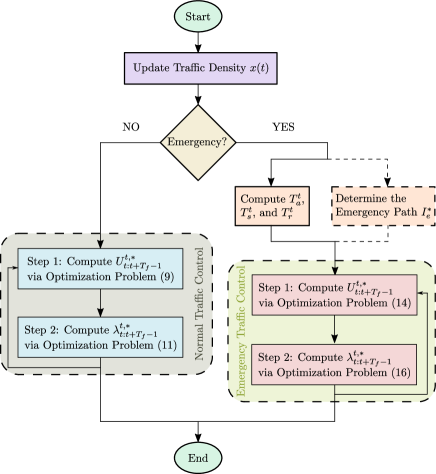
Figure 1: Algorithmic flowchart of the proposed centralized traffic control scheme. This algorithm should be run at every $t$ in the central control unit.

III-A Normal Traffic Mode

The normal traffic mode corresponds to traffic scenarios in which there is no emergency vehicle. Given the prediction horizon $[t,t+T_{f}]$, the control objective in a normal traffic mode is to determine boundary inflows and configurations of traffic lights over the prediction horizon such that traffic congestion is alleviated in all lanes. This objective can be achieved through the following two-step receding horizon control; that is, the central unit computes the optimal boundary inflows and configuration of traffic lights over the prediction horizon by solving the associated optimization problems at every time instant $t$, but only implements the next boundary inflows and configuration of traffic lights, and then solves the associated optimization problems again at the next time instant, repeatedly.

III-A1 Step 1

Consider $\{\lambda_{t:t+T_{f}-2}^{t-1,\ast},\lambda(t+T_{f}-1)\}$, where $\lambda_{t:t+T_{f}-2}^{t-1,\ast}$ is the optimal solution of (19) obtained at time $t-1$ and $\lambda(t+T_{f}-1)$ is selected randomly from the action space $\Lambda$. Then, the optimal boundary inflows over the prediction horizon $[t,t+T_{f}]$ (i.e., $U_{t:t+T_{f}-1}^{t,\ast}$) can be obtained by solving the following optimization problem:

$$\min\limits_{U}\;\sum\limits_{k=0}^{T_{f}-1}\Big{(}\left\|\hat{x}_{df}(k|t)\right\|_{\Gamma_{n}}^{2}+\left\|U(t+k)-U_{nom}(t+k)\right\|_{\Theta}^{2}\Big{)},$$ (17a)

subject to

$$\hat{x}(k|t)\subseteq\hat{\mathcal{X}}, ~{}k=1,\cdots,T_{f},$$ (17b)

$$U(t+k)\in\mathbb{Z}_{\geq 0}^{N_{in}}, ~{}k=0,\cdots,T_{f}-1,$$ (17c)

where $\Theta=\Theta^{\top}\geq 0$ ($\in\mathbb{R}^{N_{in}\times N_{in}}$) is a weighting matrix, $\hat{\mathcal{X}}\subset\mathbb{Z}_{\geq 0}^{N}$ is a polyhedron containing the origin, and

$$\hat{x}(k+1|t)\in\Big{(}A\big{(}\lambda^{t-1,\ast}(t+k)\big{)}\hat{x}(k|t)+BU(t+k)\Big{)}\oplus\mathcal{D},$$ (18)

with initial condition $\hat{x}(0|t)=x(t)$, and $\lambda^{t-1,\ast}(t+T_{f}-1)=\lambda(t+T_{f}-1)$ which is selected randomly from the action space $\Lambda$. Note that to account for the disturbance $d(t)$, (18) uses the Minkowski set-sum of nominal predictions plus the set of all possible effects of the disturbance $d(t)$ on the traffic density. The subscript “df” in (17a) stands for disturbance-free, and $\hat{x}_{df}(k|t)$ can be computed via (18) by setting $\mathcal{D}=\{\textbf{0}\}$. The $U_{nom}(t)$ is the nominal boundary inflow at time $t$, which can be estimated based on prior traffic data. In (17), $\Gamma_{n}=\text{diag}\{\gamma_{1}^{n},\cdots,\gamma_{N}^{n}\}$, where $\gamma_{i}^{n}\geq 0,~{}\forall i\in\{1,\cdots,N\}$ is a design parameter that can be used to prioritize lanes. As suggested by the U.S. Department of Transportation [42], the prioritizing parameters can be determined according to total crashes and congestion over a specified period of time (e.g., over a 5-year period); the higher the prioritizing parameter is, the higher priority is given to the density alleviation.

In summary, Step 1 computes the optimal boundary inflows by solving the optimization problem (17), which has $T_{f}\times N_{in}$ integer decision variables constrained to be non-negative, and has $T_{f}\times N$ inequality constraints on traffic density.

III-A2 Step 2

Given $U_{t:t+T_{f}-1}^{t,\ast}$ as the optimal solution of (17) obtained at time $t$, the optimal configuration of all traffic lights over the prediction horizon $[t,t+T_{f}]$ (i.e., $\lambda_{t:t+T_{f}-1}^{t,\ast}$) can be determined by solving the following optimization problem:

$$\min\limits_{\lambda}\;\sum\limits_{k=0}^{T_{f}-1}\left\|\tilde{x}_{df}(k|t)\right\|_{\Gamma_{n}}^{2},$$ (19a)

subject to

$$\tilde{x}(k|t)\subseteq\tilde{\mathcal{X}}, ~{}k=1,\cdots,T_{f},$$ (19b)

$$\lambda(t+k)\in\Lambda, ~{}k=0,\cdots,T_{f}-1,$$ (19c)

where $\tilde{\mathcal{X}}\subset\mathbb{Z}_{\geq 0}^{N}$ is a polyhedron containing the origin, and

$$\tilde{x}(k+1|t)\in\max\Big{\{}\Big{[}A\big{(}\lambda (t+k)\big{)}\tilde{x}(k|t)$$

$$+BU^{t,\ast}(t+k)\Big{]}_{+}\oplus\mathcal{D},0\Big{\}},$$ (20)

with the initial condition, $\tilde{x}(0|t)=x(t)$. Note that $\tilde{x}_{df}(k|t)$ can be computed via (III-A2) by setting $\mathcal{D}=\{\textbf{0}\}$. Note that similar to (18), a set-valued prediction of traffic density by taking into account all possible realizations of the disturbance $d(t)$ is considered in (III-A2) to account for the disturbance $d(t)$.

In summary, Step 2 determines the optimal configuration of traffic lights across the network by solving the optimization problem (19) which has $T_{f}$ decision variables (each one is an $M$-tuple representing the configuration of traffic lights) constrained to belong to the set $\Lambda$ (see Subsection II-B), and has $T_{f}\times N$ inequality constraints on traffic density.

Remark III.1

The cost function in (17) has two terms. The first term penalizes traffic density in all lanes of the network, and the second term penalizes the difference between the inlet traffic flows and their nominal values. It should be noted that a sufficiently large matrix $\Theta$ guarantees that vehicles will never be blocked behind the network gates. A different method [19] to ensure that vehicles will not be blocked is to constrain the total boundary inflow to be equal to a certain amount, i.e., $\sum_{i\in\mathcal{N}_{in}}u_{i}(t)=\bar{u},~{}\forall t$, where $\bar{u}$ can be determined based upon prior traffic data. It is noteworthy that the computed optimal inflows can be implemented by means of network gates, i.e., ramp meters [37, 38] for highways and metering gates [39] for urban streets).

Remark III.2

The prediction given in (18) provides an approximation to system (16), and the traffic density may take non-integer and/or negative values. However, as will be shown later, this approximation is efficient in ensuring optimality. The main advantage of using such an approximation is that the integer programming as in (17) can be easily solved by available tools.

Remark III.3

The optimization problem (19) can be solved by using the brute-force search [43] (a.k.a. exhaustive search or generate&test) algorithm. Note that the size of the problem (19) is limited, since $\Lambda^{T_{f}}$ and $\mathcal{D}$ are finite. However, there are some techniques to reduce the search space, and consequently speed up the algorithm. For instance, if the configuration $\lambda_{t:t+T_{f}-1}^{t}$ is infeasible and causes congestion at time $t+k$ (with $0\leq k\leq T_{f}-1$), all configurations with the same first $k-1$ actions will be excluded from the search space. Our simulation studies show that this simple step can largely reduce the computation time of the optimization problem (19) (in our case, from 10 seconds to 8 milliseconds).

Remark III.4

In the case of uncontrolled boundary inflow, the proposed scheme for normal traffic mode reduces to solving only the optimization problem (19) based upon learnt nominal boundary inflows.

Remark III.5

We assume that constraints on the traffic density are defined such that the resulting optimization problems are feasible. However, in the case of infeasibility, we can use standard methods (e.g., introducing slack variables) to relax constraints.

III-B Emergency Traffic Mode

Suppose that:

• At time $t=t_{e}$, a notification is received by the central control unit indicating that an emergency vehicle will enter the network in $T_{a}^{t}$ time steps. Note that for $t<t_{e}$ the condition of the network was normal.

• Given the entering and leaving lanes, let $\mathcal{P}$ represents the set of all possible paths for the emergency vehicle. Once the notification is received, i.e., at time $t=t_{e}$, based on the current and predicted traffic conditions, the optimal emergency path $I_{e}^{\ast}$ should be selected by the central control unit (see Remark III.10) and be given to the emergency vehicle. We assume that the emergency vehicle will follow the provided path.

• The emergency vehicle should leave the network in maximum $T_{s}^{t}$ time steps.

• Once the emergency vehicle leaves the network, the traffic density in all lanes should be recovered to the normal traffic mode in $T_{r}^{t}$ time steps. This phase will be referred as the recovery phase in the rest of the paper.

Remark III.6

$T_{a}^{t}$, $T_{s}^{t}$, and $T_{r}^{t}$ are specified at time $t$. These values can be computed by leveraging connectivity between the emergency vehicle and the roadside infrastructure. Note that these variables are time-variant, as they should be recomputed based on the traffic condition and position of the emergency vehicle at any $t$. For instance, once the emergency vehicle enters the network, $T_{a}^{t}$ should be set to zero, and once the emergency vehicle leaves the network $T_{s}^{t}$ should be set to zero. Also, when the recovery phase ends, $T_{r}^{t}$ will be zero.

The control objective in an emergency traffic mode is to shorten the traveling time of the emergency vehicle, i.e., to help the emergency vehicle traverse the network as quickly and efficiently as possible. Given the emergency path with length $L$, the traveling time of the emergency vehicle can be estimated [44, 45] as

$$\text{Traveling Time}=\frac{L}{V_{d}}+\beta\times\text{Traffic Density on the Path},$$ (21)

for some constant $\beta>0$, where $V_{d}$ is the desired traverse velocity. This relationship indicates that for fixed $L$ and $V_{d}$, to shorten the traveling time of the emergency vehicle one would need to reduce the traffic density on the emergency path.

Therefore, in an emergency traffic mode, given the prediction horizon $[t,t+T_{f}]$ with $T_{f}\geq T_{a}^{t}+T_{s}^{t}+T_{r}^{t}$, the control objective can be achieved by determining boundary inflows and configuration of all traffic lights such that: i) during the time interval $[t,t+T_{a}^{t}+T_{s}^{t}]$ traffic density in emergency path should be reduced as much as possible, while traffic density in other lanes is less than a certain amount; ii) during the time interval $[t+T_{a}^{t}+T_{s}^{t},t+T_{a}^{t}+T_{s}^{t}+T_{r}^{t}]$ the traffic density in all lanes should be recovered to the normal traffic mode; and iii) during the time interval $[t+T_{a}^{t}+T_{s}^{t}+T_{r}^{t},T_{f}]$ the traffic density in all lanes should satisfy constraints of normal mode.

We propose the following two-step receding horizon control approach to satisfy the above-mentioned objectives. In this approach, the central unit computes the optimal boundary inflows and configuration of traffic lights over the prediction horizon by solving the associated optimization problems at every time instant $t$, but only implements the next boundary inflows and configuration of traffic lights, and then solves the associated optimization problems again at the next time instant, repeatedly.

III-B1 Step 1

Consider $\{\lambda_{t:t+T_{f}-2}^{t-1,\ast},\lambda(t+T_{f}-1)\}$, where $\lambda_{t:t+T_{f}-2}^{t-1,\ast}$ is the optimal solution of (26) obtained at time $t-1$ and $\lambda(t+T_{f}-1)$ is selected randomly from the action space $\Lambda$. Then, the optimal boundary inflows over the prediction horizon $[t,t+T_{f}]$ (i.e., $U_{t:t+T_{f}-1}^{t,\ast}$) can be computed by solving the following optimization problem:

$$\min\limits_{U}\;\sum\limits_{k=0}^{T_{f}-1}\Big{(}\left\|\hat{x}_{df}(k|t)\right\|_{\Gamma_{e}}^{2}+\left\|U(t+k)-U_{nom}(t+k)\right\|_{\Theta}^{2}\Big{)},$$ (22a)

subject to

$$\hat{x}(k|t)\subseteq\hat{\mathcal{X}}^{+}, ~{}k=1,\cdots,T_{a}^{t}+T_{s}^{t}+T_{r}^{t}$$ (22b)

$$\hat{x}(k|t)\subseteq\hat{\mathcal{X}}, ~{}k=T_{a}^{t}+T_{s}^{t}+T_{r}^{t}+1,\cdots,T_{f}$$ (22c)

$$U(t+k)\in\mathbb{Z}_{\geq 0}^{N_{in}}, ~{}k=0,\cdots,T_{f}-1,$$ (22d)

where $\hat{x}(k|t)$ is as in (18), $\hat{\mathcal{X}}^{+}\supset\hat{\mathcal{X}}$ is the extended constraint set (see Remark III.8), and $\Gamma_{e}=\text{diag}\{\gamma_{1}^{e}(k),\cdots,\gamma_{N}^{e}(k)\}$ (see Remark III.9) with

$$\gamma_{i}^{e}(k)=\left\{\begin{array}[]{ll}\bar{\gamma}_{e},&\text{if $i\in I_{e}^{\ast}$ and $k\leq T_{a}^{t}+T_{s}^{t}$}\\ \gamma_{i}^{n},&\text{otherwise}\end{array}\right.,$$ (25)

with $\bar{\gamma}_{e}\gg\max_{i}\{\gamma_{i}^{n}\}$, and $I_{e}^{\ast}$ is the selected emergency path (see Remark III.10). The prioritizing parameters as in (25) ensure that the traffic density in the lanes included in the emergency path will be alleviated with a higher priority in the emergency traffic mode.

Similar to (17), the optimization problem (22) has $T_{f}\times N_{in}$ integer decision variables constrained to be non-negative, and has $T_{f}\times N$ inequality constraints on traffic density.

III-B2 Step 2

Given $U_{t:t+T_{f}-1}^{t,\ast}$ as the optimal solution of (22) obtained at time $t$, the optimal configurations of the traffic lights over the prediction horizon $[t,t+T_{f}]$ (i.e., $\lambda_{t:t+T_{f}-1}^{t,\ast}$) can be determined by solving the following optimization problem:

$$\min\limits_{\lambda}\;\sum\limits_{k=0}^{T_{f}-1}\left\|\tilde{x}_{df}(k|t)\right\|_{\Gamma_{e}}^{2},$$ (26a)

subject to

$$\tilde{x}(k|t)\subseteq\tilde{\mathcal{X}}^{+}, ~{}k=1,\cdots,T_{a}^{t}+T_{s}^{t}+T_{r}^{t},$$ (26b)

$$\tilde{x}(k|t)\subseteq\tilde{\mathcal{X}}, ~{}k=T_{a}^{t}+T_{s}^{t}+T_{r}^{t}+1,\cdots,T_{f}$$ (26c)

$$\lambda(t+k)\in\Lambda, ~{}k=0,\cdots,T_{f}-1$$ (26d)

where $\tilde{x}(k|t)$ is as in (III-A2), and $\tilde{\mathcal{X}}^{+}\supset\tilde{\mathcal{X}}$ is the extended set (see Remark III.8). Similar to (19), the optimization problem (26) has $T_{f}$ decision variables (each one is an $M$-tuple representing the configuration of traffic lights) constrained to belong to the set $\Lambda$ (see Subsection II-B), and has $T_{f}\times N$ inequality constraints on traffic density.

Remark III.7

The optimization problem (22) can be solved by mixed-integer tools, and the optimization problem (26) can be solved by using the brute-force search algorithms.

Remark III.8

We assume that constraints on the traffic density can be temporarily relaxed. This assumption is reasonable [46, 47], as in practice, constraints are often imposed conservatively to avoid congestion. In mathematical terms, by relaxation we mean that traffic density should belong to extended sets $\hat{\mathcal{X}}^{+}\supset\hat{\mathcal{X}}$ and $\tilde{\mathcal{X}}^{+}\supset\tilde{\mathcal{X}}$. This relaxation enables the control scheme to put more efforts on alleviation of traffic density in emergency path. This relaxation can last up to maximum $T_{a}^{t_{e}}+T_{s}^{t_{e}}+T_{r}^{t_{e}}$ time steps.

Remark III.9

$\Gamma_{e}$ as in (25) prioritizes alleviating traffic density in lanes included in the emergency path $I_{e}^{\ast}$ during the time interval in which the emergency vehicle is traversing the network, i.e., the time interval $[t,t+T_{a}^{t}+T_{s}^{t}]$.

Remark III.10

Once the emergency notification is received by the central control unit (i.e., at time $t=t_{e}$), the optimization problems (22) and (26) should be solved for all possible paths, i.e., for each element of $\mathcal{P}$. Then: i) according to (21), the optimal emergency path $I_{e}^{\ast}$ should be selected as

$$I_{e}^{\ast}=\arg\;\min\limits_{I_{e}\in\mathcal{P}}\;\sum\limits_{k=1}^{T_{a}^{t_{e}}+T_{s}^{t_{e}}}\sum\limits_{i\in I_{e}}x_{i,df}(k|t_{e});$$ (27)

and ii) the boundary inflow and configuration of traffic lights at time $t=t_{e}$ will be the ones associated with the optimal emergency path $I_{e}^{\ast}$.

Remark III.11

Once the recovery phase ends, the traffic condition will be normal, and the boundary inflow vector and configuration of traffic lights should be determined through the two-step control scheme presented in Subsection III-A

Remark III.12

In the case of uncontrolled boundary inflow, the proposed scheme for emergency traffic mode reduces to solving only the optimization problem (26) based upon learnt nominal boundary inflows.

IV Emergency Vehicle-Centered Traffic Control—Decentralized Scheme

In this section, we will develop a decentralized traffic control scheme whose algorithmic flowchart is depicted in Fig. 2. In decentralized scheme, there is a control unit at each intersection, which controls configuration of the traffic lights at that intersection, as well as the traffic flow in the corresponding inlets. During each sampling period, an aggregator receives data from all control units, augments data, and shares across the network. This is reasonable for real-time applications even with cheap and relatively high-latency communication technologies, as the duration of the traffic light states is large (e.g., 30 seconds). In Section V, we will characterize the optimality of the developed decentralized scheme in our numerical experiments in different traffic modes in comparison with the centralized scheme.

The main advantage of the decentralized scheme is that the size of resulting optimization problem is very small compared to that of centralized scheme, as it only needs to determine the configuration of traffic lights and inlet traffic flows at one intersection. This greatly reduces the computation time for large networks, even though it may slightly degrade performance. This will be discussed in Section V.

In this section, we use ${}^{j}x(t)\in\mathbb{R}^{N_{j}},~{}j\in\mathcal{M}$ (with $N_{j}\leq N$) to denote traffic density in lanes controlled by Control Unit#$j$. Also, ${}^{j}U_{t:t+T_{f}-1}^{t}=[^{j}U^{t}(t)^{\top}~{}\cdots~{}^{j}U^{t}(t+T_{f}-1)^{\top}]^{\top}\in\mathbb{Z}_{\geq 0}^{T_{f}N^{j}_{in}},~{}j\in\mathcal{M}$, where ${}^{j}U^{t}(t+k)\in\mathbb{Z}_{\geq 0}^{N^{j}_{in}}$ is the traffic flows in inlets associated with intersection $I_{j}$ for time $t+k$ (with $k\leq T_{f}-1$) computed at time $t$, and ${}^{j}\lambda_{t:t+T_{f}-1}^{t}=\{\lambda_{j}^{t}(t),\cdots,\lambda_{j}^{t}(t+T_{f}-1)\}\in\Lambda_{j}^{T_{f}},~{}j\in\mathcal{M}$, where $\lambda_{j}^{t}(t+k)$ is the configuration of traffic lights at intersection $I_{j}$ for time $t+k$ (with $k\leq T_{f}-1$) computed at time $t$. Note that $\sum_{j}N_{in}^{j}=N_{in}$, and $\ast$ in the superscript of the above-mentioned notations indicates optimal decisions.

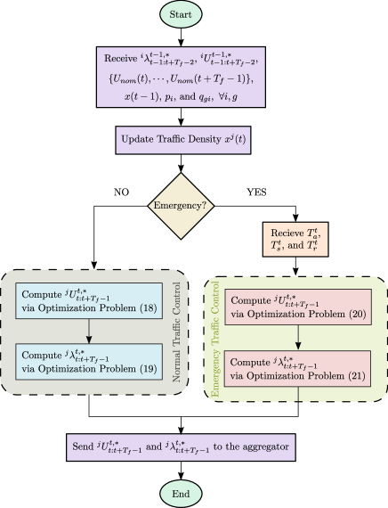
Figure 2: Algorithmic flowchart of the proposed decentralized traffic control scheme. This algorithm should be run at every $t$ in the Control Unit#$j$.

IV-A Normal Traffic Mode

As discussed in Subsection III-A, the control objective in a normal traffic mode is to alleviate traffic density across the network. During the time interval $[t-1,t)$, all control units receive ${}^{i}\lambda_{t-1:t+T_{f}-2}^{t-1,\ast}$ and ${}^{i}U_{t-1:t+T_{f}-2}^{t-1,\ast}$ for all $i\in\mathcal{M}$, $x(t-1)$, $\{U_{nom}(t),\cdots,U_{nom}(t+T_{f}-1)\}$, and $p_{i}$ and $q_{g,i},~{}i,g\in\mathcal{N}$ from the aggregator. At any $t$, the Control Unit#$j,~{}j\in\mathcal{M}$ follows the following steps to determine the inlet traffic flows and the configuration of the traffic lights at intersection $I_{j}$ in a normal traffic mode:

1. Compute $x(t|t-1)$ based on the shared information by the aggregator, and according to (16) with $d(t-1)=0$.

2. Update traffic density at local lanes (i.e., ${}^{j}x(t)$), and replace corresponding elements in $x(t|t-1)$ with updated values.

3. Compute $\{^{i}\lambda_{t:t+T_{f}-2}^{t-1,\ast},\lambda_{i}(t+T_{f}-1)\}$ for all $i\in\mathcal{M}$, where ${}^{i}\lambda_{t:t+T_{f}-2}^{t-1,\ast}$ is the optimal solution of Control Unit#$i$ obtained at time $t-1$ and $\lambda_{i}(t+T_{f}-1)$ is selected randomly from the action space $\Lambda_{i}$.

4. Compute $\{^{i}U_{t:t+T_{f}-2}^{t-1,\ast},^{i}U_{nom}(t+T_{f}-1)\}$ for all $i\in\mathcal{M}$ and $i\neq j$, where ${}^{i}U_{t:t+T_{f}-2}^{t-1,\ast}$ is the optimal solution of Control Unit#$i$ obtained at time $t-1$.

5. Solve the following optimization problem to determine the inlet traffic flows at intersection $I_{j}$ over the prediction horizon $[t,t+T_{f}]$ (i.e., ${}^{j}U_{t:t+T_{f}-1}^{t,\ast}$):

   $$\min\limits_{{}^{j}U}\;\sum\limits_{k=0}^{T_{f}-1}\Big{(} \left\|{}^{j}\hat{x}_{df}(k|t)\right\|_{{}^{j}\Gamma_{n}}^{2}$$

   $$+\left\|{}^{j}U(t+k)-~{}^{j}U_{nom}(t+k)\right\|_{{}^{j}\Theta}^{2}\Big{)},$$ (28a)

   subject to

   $${}^{j}\hat{x}(k|t)\subseteq~{}^{j}\hat{\mathcal{X}}, ~{}k=1,\cdots,T_{f},$$ (28b)

   $${}^{j}U(t+k)\in\mathbb{Z}_{\geq 0}^{N_{in}^{j}}, ~{}k=0,\cdots,T_{f}-1,$$ (28c)

   where ${}^{j}\Gamma_{n}=~{}^{j}\Gamma_{n}^{\top}\geq 0$ ($\in\mathbb{R}^{N_{j}}$) and ${}^{j}\Theta=~{}^{j}\Theta^{\top}\geq 0$ ($\in\mathbb{R}^{N_{in}^{j}\times N_{in}^{j}}$) are weighting matrices, ${}^{j}\hat{x}(k|t)$ can be computed via (18) with initial condition $x(t|t-1)$, and ${}^{j}\hat{\mathcal{X}}\subset\mathbb{R}_{\geq 0}^{N_{j}}$ is a polyhedron containing the origin. The optimization problem (28) has $T_{f}\times N_{in}^{j}$ integer decision variables constrained to be non-negative, and has $T_{f}\times N_{j}$ inequality constraints on traffic density.

6. Given ${}^{j}U_{t:t+T_{f}-1}^{t,\ast}$ as the optimal solution of (28) obtained at time $t$, solve the following optimization problem to determine the configuration of traffic lights at intersection $I_{j}$ over the prediction horizon $[t,t+T_{f}]$ (i.e., ${}^{j}\lambda_{t:t+T_{f}-1}^{t,\ast}$):

   $$\min\limits_{\lambda_{j}}\;\sum\limits_{k=0}^{T_{f}-1}\left\|{}^{j}\tilde{x}_{df}(k|t)\right\|_{\Gamma_{n}^{j}}^{2},$$ (29a)

   subject to

   $${}^{j}\tilde{x}(k|t)\subseteq~{}^{j}\tilde{\mathcal{X}}, ~{}k=1,\cdots,T_{f},$$ (29b)

   $$\lambda_{j}(t+k)\in\Lambda_{j}, ~{}k=0,\cdots,T_{f}-1,$$ (29c)

   where ${}^{j}\tilde{x}(k|t)$ can be computed via (III-A2) with initial condition $x(t|t-1)$, and ${}^{j}\tilde{\mathcal{X}}\subset\mathbb{R}_{\geq 0}^{N_{j}}$ is a polyhedron containing the origin. The optimization problem (29) has $T_{f}$ decision variables constrained to belong to the set $\Lambda_{j}$ (see Subsection II-B), and has $T_{f}\times N_{j}$ inequality constraints on traffic density.

Note that the above-mentioned scheme is receding horizon control-based; that is the Control Unit#$j,~{}j\in\mathcal{M}$ computes the optimal inlet traffic flows and configuration of the traffic lights at intersection $I_{j}$ over the prediction horizon by solving the associated optimization problems at every time instant $t$, but only implements the next inlet traffic flows and configuration of traffic lights, and then solves the associated optimization problems again at the next time instant, repeatedly.

Remark IV.1

The optimization problem (28) can be solved by mixed-integer tools, and the optimization problem (29) can be solved by using the brute-force search algorithms.

Remark IV.2

In decentralized scheme, Control Unit#$j,~{}j\in\mathcal{M}$ estimates the traffic density at time $t$ across the network by assuming $d(t-1)=0$. Thus, in general, $x(t|t-1)\neq x(t)$. Also, Control Unit#$j$ determines the optimal decisions over the prediction horizon based upon the optimal decisions of other control units at time $t-1$. As a result, the decentralized scheme is expected to provide a sub-optimal solution. This will be shown in Section V.

IV-B Emergency Traffic Mode

Consider the assumptions mentioned in Subsection III-B regarding the arriving, leaving, and recovery times. The control objective in an emergency traffic mode is to shorten the traveling time of the emergency vehicle, without causing congestion in other lanes. Given $T_{a}^{t}$, $T_{s}^{t}$, and $T_{r}^{t}$ by the aggregator, the Control Unit#$j,~{}j\in\mathcal{M}$ executes the following steps to determine the inlet traffic flows and configuration of the traffic lights at intersection $I_{j}$ in an emergency traffic mode. Note that the following scheme is receding horizon control-based; that is the Control Unit#$j,~{}j\in\mathcal{M}$ computes the optimal inlet traffic flows and configuration of the traffic lights at intersection $I_{j}$ over the prediction horizon by solving the associated optimization problems at every time instant $t$, but only implements the next inlet traffic flows and configuration of traffic lights, and then solves the associated optimization problems again at the next time instant, repeatedly.

1. Compute $x(t|t-1)$ based on the shared information by the aggregator, and according to (16) with $d(t-1)=0$.

2. Update traffic density at local lanes (i.e., ${}^{j}x(t)$), and replace corresponding elements in $x(t|t-1)$ with updated values.

3. Compute $\{^{i}\lambda_{t:t+T_{f}-2}^{t-1,\ast},\lambda_{i}(t+T_{f}-1)\}$ for all $i\in\mathcal{M}$, where ${}^{i}\lambda_{t:t+T_{f}-2}^{t-1,\ast}$ is the optimal solution of Control Unit#$i$ obtained at time $t-1$ and $\lambda_{i}(t+T_{f}-1)$ is selected randomly from the action space $\Lambda_{i}$.

4. Compute $\{^{i}U_{t:t+T_{f}-2}^{t-1,\ast},^{i}U_{nom}(t+T_{f}-1)\}$ for all $i\in\mathcal{M}$ and $i\neq j$, where ${}^{i}U_{t:t+T_{f}-2}^{t-1,\ast}$ is the optimal solution of Control Unit#$i$ obtained at time $t-1$.

5. Solve the following optimization problem to determine the inlet traffic flows at intersection $I_{j}$ over the prediction horizon $[t,t+T_{f}]$ (i.e., ${}^{j}U_{t:t+T_{f}-1}^{t,\ast}$):

   $$\min\limits_{{}^{j}U}\;\sum\limits_{k=0}^{T_{f}-1}\Big{(} \left\|{}^{j}\hat{x}_{df}(k|t)\right\|_{{}^{j}\Gamma_{e}}^{2}$$

   $$+\left\|{}^{j}U(t+k)-~{}^{j}U_{nom}(t+k)\right\|_{{}^{j}\Theta}^{2}\Big{)},$$ (30a)

   subject to

   $${}^{j}\hat{x}(k|t)\subseteq~{}^{j}\hat{\mathcal{X}}^{+}, ~{}k=1,\cdots,T_{a}^{t}+T_{s}^{t}+T_{r}^{t},$$ (30b)

   $${}^{j}\hat{x}(k|t)\subseteq~{}^{j}\hat{\mathcal{X}}, ~{}k=T_{a}^{t}+T_{s}^{t}+T_{r}^{t}+1,\cdots,T_{f},$$ (30c)

   $${}^{j}U(t+k)\in\mathbb{Z}_{\geq 0}^{N_{in}^{j}}, ~{}k=0,\cdots,T_{f}-1,$$ (30d)

   where ${}^{j}\hat{\mathcal{X}}^{+}\supset~{}^{j}\hat{\mathcal{X}}$ is the extended set (see Remark III.8), and ${}^{j}\Gamma_{e}=~{}^{j}\Gamma_{e}^{\top}\geq 0$ ($\in\mathbb{R}^{N_{j}}$) is the weighting matrix (see Remark III.9). Similar to (28), the optimization problem (30) has $T_{f}\times N_{in}^{j}$ integer decision variables constrained to be non-negative, and has $T_{f}\times N_{j}$ inequality constraints on traffic density.

6. Given ${}^{j}U_{t:t+T_{f}-1}^{t,\ast}$ as the optimal solution of (30) obtained at time $t$, solve the following optimization problem to determine the configuration of traffic lights at intersection $I_{j}$ over the prediction horizon $[t,t+T_{f}]$ (i.e., ${}^{j}\lambda_{t:t+T_{f}-1}^{t,\ast}$):

   $$\min\limits_{\lambda_{j}}\;\sum\limits_{k=0}^{T_{f}-1}\left\|{}^{j}\tilde{x}_{df}(k|t)\right\|_{\Gamma_{e}^{j}}^{2},$$ (31a)

   subject to

   $${}^{j}\tilde{x}(k|t)\subseteq~{}^{j}\tilde{\mathcal{X}}^{+}, ~{}k=1,\cdots,T_{a}^{t}+T_{s}^{t}+T_{r}^{t},$$ (31b)

   $${}^{j}\tilde{x}(k|t)\subseteq~{}^{j}\tilde{\mathcal{X}}, ~{}k=T_{a}^{t}+T_{s}^{t}+T_{r}^{t}+1,\cdots,T_{f},$$ (31c)

   $$\lambda_{j}(t+k)\in\Lambda_{j}, ~{}k=0,\cdots,T_{f}-1,$$ (31d)

   where ${}^{j}\tilde{\mathcal{X}}^{+}\supset~{}^{j}\tilde{\mathcal{X}}$ is the extended set (see Remark III.8). Similar to (29), the optimization problem (31) has $T_{f}$ decision variables constrained to belong to the set $\Lambda_{j}$ (see Subsection II-B), and has $T_{f}\times N_{j}$ inequality constraints on traffic density.

Remark IV.3

The optimization problem (30) can be solved by mixed-integer tools, and the optimization problem (31) can be solved by using the brute-force search algorithms.

Remark IV.4

In decentralized scheme the emergency path $I_{e}^{\ast}$ is determined by the emergency vehicle, and is shared with control units through the aggregator.

Remark IV.5

In this paper we assume that each control unit in the decentralized scheme controls the inlet traffic flows and configuration of traffic lights at one intersection. However, the decentralized scheme is applicable to the case where a network is divided into some sub-networks, and there exist a control unit in each sub-network controlling the entire sub-network.

V Simulation Results

Consider the traffic network shown in Fig. 3. This network contains 14 unidirectional lanes identified by the set $\mathcal{N}=\{1,\cdots,14\}$, and 4 intersections identified by the set $\mathcal{M}=\{1,\cdots,4\}$. Also, $\mathcal{N}_{in}=\{2,7,8\}$. The edge set is $\mathcal{E}=\{(2,3),(2,11),(7,12),(7,14),(7,6),(8,1),(8,10),(8,13),\allowbreak(10,3),(10,11),(11,4),(11,5),(12,1),(12,9),(12,10),\allowbreak(13,6),(13,14),(14,4),(14,5)\}$.

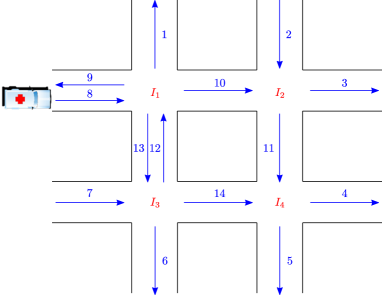
Figure 3: Considered traffic network with 14 lanes and 4 intersections. An emergency vehicle enters through lane 8 and leaves through lane 5.

Fig. 4 shows possible configurations of traffic lights at each intersection of the traffic network shown in Fig. 3. As seen in this figure, $\mu_{1}=\mu_{2}=\mu_{3}=\mu_{4}=2$, and the possible configurations at each intersection are: i) Intersection $I_{1}$: $\lambda_{1,1}$ corresponds to a ‘green’ light at the end of lane 8, and a ‘red’ light at the end of lane 12; $\lambda_{1,2}$ corresponds to a ‘red’ light at the end of lane 8, and a ‘green’ light at the end of lane 12; ii) Intersection $I_{2}$: $\lambda_{2,1}$ corresponds to a ‘green’ light at the end of lane 10, and a ‘red’ light at the end of lane 2; $\lambda_{2,2}$ corresponds to a ‘red’ light at the end of lane 10, and a ‘green’ light at the end of lane 2; iii) Intersection $I_{3}$: $\lambda_{3,1}$ corresponds to a ‘green’ light at the end of lane 7, and a ‘red’ light at the end of lane 13; $\lambda_{3,2}$ corresponds to a ‘red’ light at the end of lane 7, and a ‘green’ light at the end of lane 13; and iv) Intersection $I_{4}$: $\lambda_{4,1}$ corresponds to a ‘green’ light at the end of lane 14, and a ‘red’ light at the end of lane 11; $\lambda_{4,2}$ corresponds to a ‘red’ light at the end of lane 14, and a ‘green’ light at the end of lane 11.

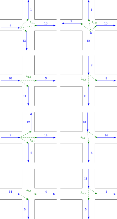
Figure 4: Possible configurations of traffic lights at each intersection of the considered traffic network. The action space is $\Lambda=\Lambda_{1}\times\Lambda_{2}\times\Lambda_{3}\times\Lambda_{4}$, where $\Lambda_{1}=\{\lambda_{1,1},\lambda_{1,2}\}$, $\Lambda_{2}=\{\lambda_{2,1},\lambda_{2,2}\}$, $\Lambda_{3}=\{\lambda_{3,1},\lambda_{3,2}\}$, and $\Lambda_{4}=\{\lambda_{4,1},\lambda_{4,2}\}$.

The boundary inflow vector of the traffic network shown in Fig. 3 is $U(t)=[u_{2}(t)~{}u_{7}(t)~{}u_{8}(t)]^{\top}\in\mathbb{Z}_{\geq 0}^{3}$. We assume that $\Delta T=30$ seconds; this sampling period is appropriate to address macroscopic characteristics of traffic flow [19, 48, 49], as the traffic cycle ranges from one minute to three minutes in real-world systems [31]. For intersection $I_{1}$ and for the action $\lambda=(\lambda_{1,1},\lambda_{2},\lambda_{3},\lambda_{4})$, we have $p_{8}(\lambda)\in[0,1]$, $p_{12}(\lambda)=0$, $q_{8,1}(\lambda),q_{8,10}(\lambda),q_{8,13}(\lambda)\in[0,1]$, and $q_{12,1}(\lambda)=q_{12,9}(\lambda)=q_{12,10}(\lambda)=0$. For intersection $I_{1}$ and for the action $\lambda=(\lambda_{1,2},\lambda_{2},\lambda_{3},\lambda_{4})$, we have $p_{8}(\lambda)=0$, $p_{12}(\lambda)\in[0,1]$, $q_{8,1}(\lambda),q_{8,10}(\lambda),q_{8,13}(\lambda)=0$, and $q_{12,1}(\lambda)=q_{12,9}(\lambda)=q_{12,10}(\lambda)\in[0,1]$. For intersection $I_{2}$ and for the action $\lambda=(\lambda_{1},\lambda_{2,1},\lambda_{3},\lambda_{4})$, we have $p_{10}(\lambda)\in[0,1]$, $p_{2}(\lambda)=0$, $q_{10,3}(\lambda),q_{10,11}(\lambda)\in[0,1]$, and $q_{2,3}(\lambda)=q_{2,11}(\lambda)=0$. For intersection $I_{2}$ and for the action $\lambda=(\lambda_{1},\lambda_{2,2},\lambda_{3},\lambda_{4})$, we have $p_{10}(\lambda)=0$, $p_{2}(\lambda)\in[0,1]$, $q_{10,3}(\lambda),q_{10,11}(\lambda)=0$, and $q_{2,3}(\lambda)=q_{2,11}(\lambda)\in[0,1]$. For intersection $I_{3}$ and for the action $\lambda=(\lambda_{1},\lambda_{2},\lambda_{3,1},\lambda_{4})$, we have $p_{13}(\lambda)=0$, $p_{7}(\lambda)\in[0,1]$, $q_{13,6}(\lambda),q_{13,14}(\lambda)=0$, and $q_{7,12}(\lambda)=q_{7,14}(\lambda)=q_{7,6}(\lambda)\in[0,1]$. For intersection $I_{3}$ and for the action $\lambda=(\lambda_{1},\lambda_{2},\lambda_{3,2},\lambda_{4})$, we have $p_{13}(\lambda)\in[0,1]$, $p_{7}(\lambda)=0$, $q_{13,6}(\lambda),q_{13,14}(\lambda)\in[0,1]$, and $q_{7,12}(\lambda)=q_{7,14}(\lambda)=q_{7,6}(\lambda)=0$. For intersection $I_{4}$ and for the action $\lambda=(\lambda_{1},\lambda_{2},\lambda_{3},\lambda_{4,1})$, we have $p_{14}(\lambda)\in[0,1]$, $p_{11}(\lambda)=0$, $q_{14,4}(\lambda),q_{14,5}(\lambda)\in[0,1]$, and $q_{11,4}(\lambda)=q_{11,5}(\lambda)=0$. For intersection $I_{4}$ and for the action $\lambda=(\lambda_{1},\lambda_{2},\lambda_{3},\lambda_{4,2})$, we have $p_{14}(\lambda)=0$, $p_{11}(\lambda)\in[0,1]$, $q_{14,4}(\lambda),q_{14,5}(\lambda)=0$, and $q_{11,4}(\lambda)=q_{11,5}(\lambda)\in[0,1]$.

For implementing the decentralized scheme, we assume ${}^{1}x(t)=[x_{1}(t)~{}x_{8}(t)~{}x_{9}(t)~{}x_{12}(t)]^{\top}\in\mathbb{Z}_{\geq 0}^{4}$, ${}^{2}x(t)=[x_{2}(t)~{}x_{3}(t)~{}x_{10}(t)]^{\top}\in\mathbb{Z}_{\geq 0}^{3}$, ${}^{3}x(t)=[x_{6}(t)~{}x_{7}(t)~{}x_{13}(t)]^{\top}\in\mathbb{Z}_{\geq 0}^{3}$, and ${}^{4}x(t)=[x_{4}(t)~{}x_{5}(t)~{}x_{11}(t)~{}x_{14}(t)]^{\top}\in\mathbb{Z}_{\geq 0}^{4}$. That is Control Unit#1 controls lanes 1, 8, 9, and 12; Control Unit#2 controls lanes 2, 3, and 10; Control Unit#3 controls lanes 6, 7, and 13; and Control Unit#4 controls lanes 4, 5, 11, and 14. Also, ${}^{1}U(t)=u_{8}(t)$, ${}^{2}U(t)=u_{2}(t)$, and ${}^{3}U(t)=u_{7}(t)$. Thus, $N_{in}^{1}=1$, $N_{in}^{2}=1$, $N_{in}^{3}=1$, and $N_{in}^{4}=0$.

The simulations are run on an Intel(R) Core(TM) i7-7500U CPU 2.70 GHz with 16.00 GB of RAM. In order to have a visual demonstration of the considered traffic network, a simulator is generated (see Fig. 5). A video of operation of the simulator is available at the URL: https://youtu.be/FmEYCxmD-Oc. For comparison purposes, we also simulate the centralized scheme presented in [19] and a typical/existing/usual/baseline traffic system (i.e., the system with periodic schedule for traffic lights). TABLE II compares the mean Computation Time (CT) of the proposed schemes per time step with that of the scheme presented in [19], where the value for the scheme of [19] is used as the basis for normalization. As can be seen from this table, the computation time of the proposed centralized scheme is $\sim 1.5$ times less than that of the scheme of [19]. The computation time of the proposed decentralized scheme is $\sim 1000$ times less than that of the scheme of [19], and is $\sim 800$ times less than that of the proposed centralized scheme.

TABLE II: Comparing the mean computation time of the proposed schemes with that of scheme of [40].

	Centralized	Decentralized	Scheme of [19]
Mean CT (Norm.)	$0.734$	$1.03\times 10^{-3}$	$1$

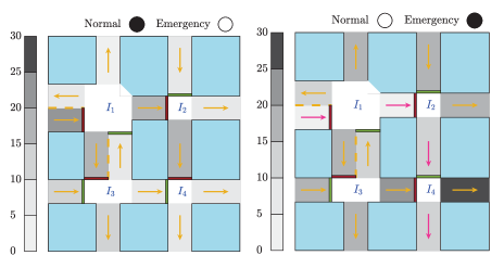
Figure 5: A screenshot of the generated simulator shown in the accompanied video (https://youtu.be/FmEYCxmD-Oc). The black circle at the top shows the traffic mode in the network, which is either normal or emergency. The color of each lane indicates the traffic density, which can be interpreted according to the bar at the left. Yellow arrows show traffic direction at each lane, and pink arrows show selected emergency path.

V-A Normal Traffic Mode

Let $\hat{\mathcal{X}}=\tilde{\mathcal{X}}=\{x|x_{i}\leq 20,~{}i\in\{1,\cdots,14\}\}$, and $d_{i}(t),~{}\forall i$ be selected uniformly from $\{-2,-1,0,1,2\}$. The initial condition is $x(0)=[15,16,15,12,12,17,18,10,10,14,12,10,16,10]^{\top}$, and the nominal boundary inflow is $U_{nom}(t)=[6,6,8]^{\top}$. Also, $\Theta=50I_{N_{in}}$ and $\gamma_{i}^{n}=1,~{}\forall i$.

Simulation results are shown in Fig. 6. TABLE III compares the achieved Steady-State Density (SSD) with the considered schemes, where the value for the typical/existing/usual/baseline traffic system is used as the basis for normalization. Note that the reports are based on results of 1000 runs. According to TABLE III, all methods perform better than the typical/existing/usual/baseline traffic system. The proposed centralized scheme provides the best response. The proposed decentralized scheme outperforms the scheme of [19], while as expected, it yields a larger SSD compared to the proposed centralized scheme. More precisely, degradation in the mean SSD by the decentralized scheme in comparison with the centralized scheme in a normal traffic mode is 11.42% which is small and acceptable in real-life traffic scenarios. Thus, the cost of using the decentralized scheme instead of the centralized scheme in a normal traffic mode is very small.

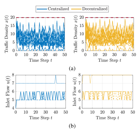
Figure 6: Simulation results for the centralized and decentralized traffic control schemes in a normal traffic mode. Figure (a): Traffic density in all lanes. Figure (b): Inlet traffic flows.

V-B Emergency Traffic Mode

Suppose that at time $t=10$, the aggregator receives a notification that an emergency vehicle will enter the network through lane 8 in two time steps, and should leave the network in two time steps through lane 5. Also, suppose that we have one time step to recover the traffic condition. We have $\mathcal{P}=\{I_{e}^{1},I_{e}^{2}\}$, where $I_{e}^{1}=\{8,13,14,5\}$ and $I_{e}^{2}=\{8,10,11,5\}$. Let $\hat{\mathcal{X}}^{+}=\tilde{\mathcal{X}}^{+}=\{x|x_{i}\leq 25\}$.

Simulation results are shown in Fig. 7, and the results from comparison analysis are reported in TABLE IV, that are computed based on results of 1000 runs. Note that the values for the typical/existing/usual/baseline traffic system are used as nominal values for normalization. As seen in TABLE IV, both schemes proposed in this paper perform better than the typical/existing/usual/baseline traffic system in an emergency traffic mode. In particular, the centralized and decentralized schemes reduce the mean SSD by 23.73% and 14.58%, respectively. As expected, the decentralized scheme yields a larger SSD compared to the centralized scheme. More precisely, degradation in mean SSD by the decentralized scheme in comparison with the centralized scheme is 11.98%. TABLE IV also reports that the centralized and decentralized schemes reduce the mean Density in Emergency Path (DEP) by 47.97% and 30.42%, respectively. It is noteworthy that the degradation in the mean DEP by the decentralized scheme in comparison with the centralized scheme is 33.73%.

TABLE III: Comparing the mean steady-state density with the considered schemes in a normal traffic mode. The value for the typical/existing/usual/baseline traffic system is used as the basis for normalization.

	Centralized	Decentralized	Scheme of [19]
Mean SSD (Norm.)	$0.7251$	$0.8079$	$0.9035$

TABLE IV: Comparing the mean steady-state density and density in emergency path with the proposed centralized and decentralized schemes in an emergency traffic mode. The values for the typical/existing/usual/baseline traffic system are used as bases for normalization.

	Centralized	Decentralized
Mean SSD (Norm.)	0.7627	0.8542
Mean DEP (Norm.)	0.5203	0.6958

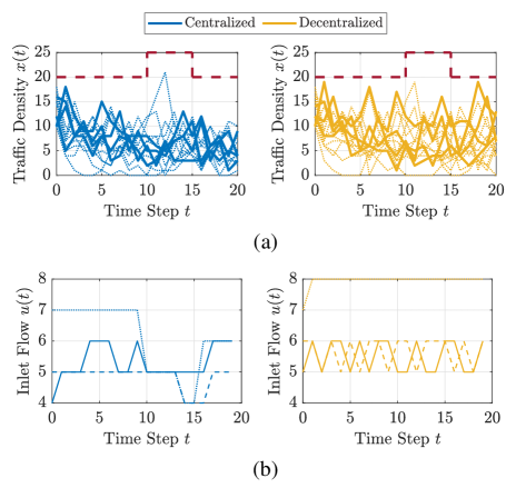
Figure 7: Simulation results for the centralized and decentralized traffic control schemes in an emergency traffic mode. Figure (a): Traffic density in all lanes. Figure (b): Inlet traffic flows.

V-C Sensitivity Analysis—Impact of Look-Ahead Horizon $T_{f}$

Fig. 8 shows how the prediction window size impacts the performance and computation time of the developed centralized scheme, where the values for $T_{f}=1$ are used as nominal values for normalization. From Fig. 8-left, we see that as the look-ahead horizon increases, the performance of the decentralized scheme improves as it takes into account more information of future conditions. However, as we look further into the future, the performance is degraded since prediction accuracy reduces. Fig. 8-right shows that as the look-ahead horizon increases, the computation time of the proposed decentralized scheme increases concomitantly with the size and complexity of the associated optimization problems. In the simulation studies, we selected $T_{f}=4$, as it yields the best performance with an affordable computing time. Note that a similar behavior is observed for the centralized scheme; that is $T_{f}=4$ provides the best performance for the centralized scheme.

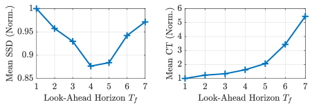
Figure 8: Impact of the look-ahead horizon $T_{f}$ on the performance and computation time of the proposed decentralized scheme, where the values for $T_{f}=1$ are used as bases for normalization. As $T_{f}$ increases the performance improves at the cost of increased computation time. For large $T_{f}$ the performance degrades due to poor prediction accuracy.

VI Conclusion

This paper proposed an emergency vehicle-centered traffic control framework to alleviate traffic congestion in a network of interconnected signaled lanes. The aim of this paper is to integrate CTM with MPC, to ensure that emergency vehicles traverse multiple intersections efficiently and timely. Two schemes were developed in this paper: i) centralized; and ii) decentralized. It was shown that the centralized scheme provides the optimal solution, even though its computation time may be large for large networks. To cope with this problem, a decentralized scheme was developed, where an aggregator acts as the hub of the network. It was shown that the computation time of the decentralized scheme is very small, which makes it a good candidate for large networks, even though it provides a sub-optimal solution. Extensive simulation studies were carried out to validate and evaluate the performance of the proposed schemes.

Future work will aim at extending the developed schemes to deal with cases where two (or more) emergency vehicles traverse a network. This extension is not trivial, and requires addressing many technical and methodological challenges. Also, future work should investigate robustness and tolerance of the decentralized scheme to uncertainty in communication delay and communication failures.

Mehdi Hosseinzadeh received his Ph.D. degree in Electrical Engineering-Control from the University of Tehran, Iran, in 2016. From 2017 to 2019, he was a postdoctoral researcher at Université Libre de Bruxelles, Brussels, Belgium. In 2018, he was a visiting researcher at University of British Columbia, Canada. He is currently a postdoctoral research associate at Washington University in St. Louis, MO, USA. His research interests include nonlinear and adaptive control, constrained control, and safe and robust control of autonomous systems.

Bruno Sinopoli received his Ph.D. in Electrical Engineering from the University of California at Berkeley, in 2005. After a postdoctoral position at Stanford University, he was the faculty at Carnegie Mellon University from 2007 to 2019, where he was full professor in the Department of Electrical and Computer Engineering with courtesy appointments in Mechanical Engineering and in the Robotics Institute and co-director of the Smart Infrastructure Institute. In 2019 he joined Washington University in Saint Louis, where he is the chair of the Electrical and Systems Engineering department. He was awarded the 2006 Eli Jury Award for outstanding research achievement in the areas of systems, communications, control and signal processing at U.C. Berkeley, the 2010 George Tallman Ladd Research Award from Carnegie Mellon University and the NSF Career award in 2010. His research interests include the modeling,analysis and design of Secure by Design Cyber-Physical Systems with applications to Energy Systems, Interdependent Infrastructures and Internet of Things.

Ilya Kolmanovsky is a professor in the department of aerospace engineering at the University of Michigan,with research interests in control theory for systems with state and control constraints, and in control applications to aerospace and automotive systems. He received his Ph.D. degree in aerospace engineering from the University of Michigan in 1995. Prof. Kolmanovsky is a Fellow of IEEE and is named as an inventor on 104 United States patents.

Sanjoy Baruah joined Washington University in St. Louis in September 2017. He was previously at the University of North Carolina at Chapel Hill (1999–2017) and the University of Vermont (1993–1999). His research interests and activities are in real-time and safety-critical system design, scheduling theory, resource allocation and sharing in distributed computing environments, and algorithm design and analysis.

References

- [1] https://www.tomtom.com/en_gb/traffic-index, accessed: .
- [2] A. Barth and U. Franke, “Tracking oncoming and turning vehicles at intersections,” in Proc. 13th Int. IEEE Conf. Intelligent Transportation Systems, Funchal, Portugal, Sep. 19-22, 2010, pp. 861–868.
- [3] P. Oza and T. Chantem, “Timely and non-disruptive response of emergency vehicles: A real-time approach,” in Proc. 29th Int. Conf. Real-Time Networks and Systems, Nantes, France, Apr. 7-9, 2021.
- [4] https://www.nena.org/page/911Statistics, accessed: .
- [5] A. B. Jena, N. C. Mann, L. N. Wedlund, and A. Olenski, “Delays in emergency care and mortality during major u.s. marathons,” N. Engl. J. Med., vol. 376, no. 15, pp. 1441–1450, Apr. 2017.
- [6] https://ops.fhwa.dot.gov/publications/fhwahop09005/move_over.htm, accessed: .
- [7] H. Hsiao, J. Chang, and P. Simeonov, “Preventing emergency vehicle crashes: Status and challenges of human factors issues,” J. Hum. Factors Ergon. Soc., vol. 60, no. 7, pp. 1048–1072, Nov. 2018.
- [8] https://injuryfacts.nsc.org/motor-vehicle/road-users/emergency-vehicles, accessed: .
- [9] V. Paruchuri, “Adaptive preemption of traffic for emergency vehicles,” in Proc. UKSim-AMSS 19th Int. Conf. Computer Modelling & Simulation, Cambridge, UK, Apr. 5-7, 2017, pp. 45–49.
- [10] W. Kang, G. Xiong, Y. Lv, X. Dong, F. Zhu, and Q. Kong, “Traffic signal coordination for emergency vehicles,” in Proc. 2014 IEEE 17th Int. Conf. Intelligent Transportation Systems, Qingdao, China, Oct. 8-11, 2014, pp. 157–161.
- [11] M. Cao, Q. Shuai, and V. O. K. Li, “Emergency vehicle-centered traffic signal control in intelligent transportation systems,” in Proc. 2019 IEEE Intelligent Transportation Systems Conf., Auckland, New Zealand, Oct. 27-30, 2019, pp. 4525–4531.
- [12] B. Kapusta, M. Miletić, E. Ivanjko, and M. Vujić, “Preemptive traffic light control based on vehicle tracking and queue lengths,” in Proc. 2017 International Symposium ELMAR, Zadar, Croatia, Sep. 18-20, 2017, pp. 11–16.
- [13] P. Oza, T. Chantem, and P. Murray-Tuite, “A coordinated spillback-aware traffic optimization and recovery at multiple intersections,” in Proc. IEEE 26th Int. Conf. Embedded and Real-Time Computing Systems and Applications, Gangnueng, Korea (South), Aug. 19-21, 2020.
- [14] S. Lin, B. D. Schutter, Y. Xi, and H. Hellendoorn, “Efficient network-wide model-based predictive control for urban traffic networks,” Transp. Res. Part C Emerg. Technol., vol. 24, pp. 122–140, Oct. 2012.
- [15] L. D. Baskar, B. D. Schutter, and H. Hellendoorn, “Traffic management for automated highway systems using model-based predictive control,” IEEE Trans. Intell. Transp. Syst., vol. 13, no. 2, pp. 838–847, Jun. 2012.
- [16] T. Tettamanti, T. Luspay, B. Kulcsár, T. Péni, and I. Varga, “Robust control for urban road traffic networks,” IEEE Trans. Intell. Transp. Syst., vol. 15, no. 1, pp. 385–398, Feb. 2014.
- [17] A. J. I. Papamichail, M. Papageorgiou, and B. D. Schutter, “Sustainable model-predictive control in urban traffic networks: Efficient solution based on general smoothening methods,” IEEE Trans. Control Syst. Technol., vol. 26, no. 3, pp. 813–827, May 2018.
- [18] S. Jafari and K. Savla, “On structural properties of optimal feedback control of traffic flow under the cell transmission model,” in Proc. 2019 American Control Conference, Philadelphia, PA, USA, Jul. 10-12, 2019, pp. 3309–3314.
- [19] H. Rastgoftar and J.-B. Jeannin, “A physics-based finite-state abstraction for traffic congestion control,” in Proc. 2021 American Control Conference, New Orleans, LA, USA, May 25-28, 2021, pp. 237–242.
- [20] C. Toy, K. Leung, L. Alvarez, and R. Horowitz, “Emergency vehicle maneuvers and control laws for automated highway systems,” IEEE Trans. Intell. Transp. Syst., vol. 3, no. 2, pp. 109–119, Jun. 2002.
- [21] R. K. Kamalanathsharma and K. L. Hancock, “Intelligent preemption control for emergency vehicles in urban corridors,” in Proc. 91st Annual Meeting Transportation Research Board, Washington DC, USA, Jan. 22-26, 2012.
- [22] M. During and P. Pascheka, “Cooperative decentralized decision making for conflict resolution among autonomous agents,” in Proc. 2014 IEEE Int. Symp. Innovations in Intelligent Systems and Applications, Alberobello, Italy, Jun. 23-25, 2014.
- [23] F. Weinert and M. During, “Development and assessment of cooperative V2X applications for emergency vehicles in an urban environment enabled by behavioral models,” in Modeling Mobility with Open Data, M. Behrisch and M. Weber, Eds. Springer, Cham, 2015, pp. 125–153.
- [24] G. J. Hannoun, P. Murray-Tuite, K. Heaslip, and T. Chantem, “Facilitating emergency response vehicles’ movement through a road segment in a connected vehicle environment,” IEEE Trans. Intell. Transp. Syst., vol. 20, no. 9, pp. 3546–3557, Sep. 2019.
- [25] J. Wu, B. Kulcsár, S. Ahn, and X. Qu, “Emergency vehicle lane pre-clearing: From microscopic cooperation to routing decision making,” Transport. Res. B Meth., vol. 141, pp. 223–239, Nov. 2020.
- [26] Y. Feng, K. L. Head, S. Khoshmagham, and M. Zamanipour, “A real-time adaptive signal control in a connected vehicle environment,” Transp. Res. Part C Emerg. Technol., vol. 55, pp. 460–473, Jun. 2015.
- [27] X. Li, Z. Zhao, L. Liu, Y. Liu, and P. Li, “An optimization model of multi-intersection signal control for trunk road under collaborative information,” J. Control. Sci. Eng., vol. 2017, p. 2846987, 2017.
- [28] P. Shao, L. Wang, W. Qian, Q. guo Wang, and X.-H. Yang, “A distributed traffic control strategy based on cell-transmission model,” IEEE Access, vol. 6, pp. 10 771–10 778, 2018.
- [29] E. F. Camacho and C. B. Alba, Model Predictive Control. Springer-Verlag London, 2007.
- [30] J. Mattingley, Y. Wang, and S. Boyd, “Code generation for receding horizon control,” in Proc. IEEE Int. Symposium on Computer-Aided Control System Design, Yokohama, Japan, Sep. 8–10, 2010, pp. 985–992.
- [31] N. A. of City Transportation Officials, “Urban street design guide,” https://nacto.org/publication/urban-street-design-guide/, accessed: .
- [32] S. Chanut and C. Buisson, “Macroscopic model and its numerical solution for two-flow mixed traffic with different speeds and lengths,” Transp. Res. Rec., vol. 1852, no. 1, pp. 209–219, Jan. 2003.
- [33] Z. H. Khan and T. A. Gulliver, “A macroscopic traffic model for traffic flow harmonization,” Eur. Transp. Res. Rev., vol. 10, 2018.
- [34] H. Yu, M. Diagne, L. Zhang, and M. Krstic, “Bilateral boundary control of moving shockwave in lwr model of congested traffic,” IEEE Trans. Autom. Control, vol. 66, no. 3, pp. 1429–1436, Mar. 2021.
- [35] L. Adacher and M. Tiriolo, “A macroscopic model with the advantages of microscopic model: A review of cell transmission model’s extensions for urban traffic networks,” Simul. Model Pract. Theory, vol. 86, pp. 102–119, Aug. 2018.
- [36] S. C. Vishnoi, S. A. Nugroho, A. F. Taha, C. Claudel, and T. Banerjee, “Asymmetric cell transmission model-based, ramp-connected robust traffic density estimation under bounded disturbances,” in Proc. 2020 American Control Conference, Denver, CO, USA, Jul. 1-3, 2020, pp. 1197–1202.
- [37] G. Gomes and R. Horowitz, “Optimal freeway ramp metering using the asymmetric cell transmission model,” Transp. Res. Part C Emerg. Technol., vol. 14, no. 4, pp. 224–262, Aug. 2006.
- [38] G. Gomes, R. Horowitz, A. A. Kurzhanskiy, P. Varaiya, and J. Kwon, “Behavior of the cell transmission model and effectiveness of ramp metering,” Transp. Res. Part C Emerg. Technol., vol. 16, no. 4, pp. 485–513, Aug. 2008.
- [39] R. Mohebifard and A. Hajbabaie, “Dynamic traffic metering in urban street networks: Formulation and solution algorithm,” Transp. Res. Part C Emerg. Technol., vol. 93, pp. 161–178, Aug. 2018.
- [40] H. Rastgoftar and E. Atkins, “An integrative data-driven physics-inspired approach to traffic congestion control,” arXiv:1912.00565 [eess.SY], Dec. 2019.
- [41] A. A. Makki, T. T. Nguyen, J. Ren, D. Al-Jumeily, and W. Hurst, “Estimating road traffic capacity,” IEEE Access, vol. 8, pp. 228 525–228 547, Nov. 2020.
- [42] U. D. of Transportation, “Analyze and prioritize individual roadway links and active traffic management strategies,” in Active Traffic Management Feasibility and Screening Guide. U.S. Department of Transportation, 2015, ch. 5.
- [43] M. Mahoor, F. R. Salmasi, and T. A. Najafabadi, “A hierarchical smart street lighting system with brute-force energy optimization,” IEEE Sens. J., vol. 17, no. 9, pp. 2871–2879, May 2017.
- [44] J. Zhao and G. Cao, “VADD: Vehicle-assisted data delivery in vehicular ad hoc networks,” IEEE Trans. Veh. Technol., vol. 57, no. 3, pp. 1910–1922, May 2008.
- [45] X. Zhang, B. Liu, and J. Tang, “A study on the tracking problem in vehicular ad hoc networks,” Int. J. Distrib. Sens. Netw., vol. 9, no. 2, p. 809742, Feb. 2013.
- [46] I. Kolmanovsky, A. Weiss, and W. Merrill, “Incorporating risk into control design for emergency operation of turbo-fan engines,” in Proc. Infotech@Aerospace conf., St. Louis, MO, USA, Mar. 29-31, 2011.
- [47] H. Li, I. Kolmanovsky, and A. Girard, “A failure mode reconfiguration strategy based on constraint admissible and recoverable sets,” in Proc. American Control conf., New Orleans, LA, USA, May 26-28, 2021.
- [48] P. B. C. van Erp, V. L. Knoop, and S. Hoogendoorn, “Macroscopic traffic state estimation using relative flows from stationary and moving observers,” Transp. Res. Part B Meth., vol. 114, pp. 281–299, Aug. 2018.
- [49] W. Wong, S. C. Wong, and H. X. Liu, “Network topological effects on the macroscopic fundamental diagram,” Transportmetrica B: Transport Dynamics, vol. 9, no. 1, pp. 376–398, 2021.