Invariant Smoothing with low process noise

Abstract

In this paper we address smoothing - that is, optimisation-based - estimation techniques for localisation problems in the case where motion sensors are very accurate. Our mathematical analysis focuses on the difficult limit case where motion sensors are infinitely precise, resulting in the absence of process noise. Then the formulation degenerates, as the dynamical model that serves as a soft constraint becomes an equality constraint, and conventional smoothing methods are not able to fully respect it. By contrast, once an appropriate Lie group embedding has been found, we prove theoretically that invariant smoothing gracefully accommodates this limit case in that the estimates tend to be consistent with the induced constraints when the noise tends to zero. Simulations on the important problem of initial alignement in inertial navigation show that, in a low noise setting, invariant smoothing may favorably compare to state-of-the-art smoothers when using precise inertial measurements units (IMU).

I Introduction

Over the past years, the smoothing approach has gained ever increasing credit as a state estimator in robotics, owing to the progresses of computers and sparse linear algebra. The rationale is to reduce the consequences of wrong linearisation points [24] through relinarisation. Many of the state-of-the-art algorithms for simultaneous localisation and mapping (SLAM) and visual odometry are based on smoothing, e.g., [32, 26]. It was more recently applied to GPS aided inertial navigation, showing promising results [31, 42, 35].

In parallel, Lie group embeddings have allowed for a new class of filters, see [30, 39, 12], and in particular the Invariant Extended Kalman Filter (IEKF) [11], in its modern form [5], see [6] for an overview. The IEKF possesses convergence guarantees [5], resolves the inconsistency issues of the EKF for SLAM, see [4] and following work [40, 14, 29, 33]. For inertial navigation, combining the IEKF with the Lie group of double spatial direct isometries $SE_{2}(3)$, or extended poses, introduced in [5], leads to powerful results. In particular, it has led to patented products, see [3, 6], and improved legged robot state estimation [28, 36]. Besides their convergence properties as observers, invariant filters also gracefully accommodate navigation systems’ uncertainty, see [13]. Leveraging the framework of Invariant filtering for smoothing, a new estimation algorithm was recently proposed, namely Invariant Smoothing (IS) [19], see also [38] and [37].

Another property of the IEKF is that it delivers “physically consistent” estimates, when some state variables are known with high degrees of certainty, see [18, 10].

In the realm of smoothing algorihtms, low noise (or equivalently high degrees of certainty) leads to two different kinds of problems:

• linear matrix inversion problems due to ill-conditioning when solving the linearised problem at each step,

• once the linearised problem is properly solved, inconsistent estimates stemming from the nonlinearity of the original problem.

The first point is solved in [20] and won’t be considered herein. The second point is the object of the current paper.

The contributions of this paper are as follows:

• Motivated by the fact that smoothing generally performs better than filtering, we provide a theory that consists of the counterpart of the results of [18, 10] in the context of smoothing.

• IS is shown to better behave than other solvers on a simple wheeled robot localisation example with deterministic dynamics, and the theory gives insight into the reasons why.

• The theory is applied to the difficult problem of alignment in inertial navigation systems (INS), i.e., IMU-GPS fusion when initial orientation is unknown [41, 22], using a high-grade IMU. Invariant smoothing (IS) favorably compares to state-of-the-art smoothing schemes [25, 23], as predicted by the theory.

The superiority of invariant filtering for alignment, discovered during A. Barrau’s thesis [3, 2], has been confirmed in multiple recent works [27, 15, 17, 16], which is the reason why it had first prompted patent filing and industrial implementations [3]. This has opened avenues for filtering-based alignment, a task generally performed through optimization (for a recent reference see [34]). However, the optimisation-based invariant approach to alignment has never been explored, as is done in the present paper.

The paper is organised as follows. In Section II we apply IS to wheeled robot localization and show in the absence of noise the behavior of IS is more meaningful than other smoothing algorithms. To explain this feature, we start off by situating the problem in Section III. Section IV presents the proposed general theory which explains the behavior observed in Section II. In Section V, the alignment problem in inertial navigation is shown to fit into the proposed framework, using the Lie group of double direct spatial isometries $SE_{2}(3)$ [5], and the theoretical results are shown to apply. Low noise simulations show the invariant smoothing approach favorably compares to state-of-the-art smoothers.

II Introductory example

Consider a wheeled mobile robot in the plane with unknown initial heading $\theta_{0}$. The state consists of its orientation and 2D position $(\theta,\mathbf{x})\in\mathbb{S}^{1}\times{\mathbb{R}}^{2}$. Let $\mathbf{R}(\theta)\in SO(2)$ denote the planar rotation of angle $\theta$. For tutorial purposes, assume the robot follows a straight line at constant velocity. This constant velocity motion writes, see e.g., [5]

$$\theta_{i+1}=\theta_{i},\quad\mathbf{x}_{i+1}=\mathbf{x}_{i}+\mathbf{R}(\theta_{i})\mathbf{u}$$ (1)

where $\mathbf{u}=\mathbf{u}_{0}dt\in{\mathbb{R}}^{2}$ with $\mathbf{u}_{0}$ the constant robot’s velocity and $dt$ the stepsize. Suppose that the robot is equipped with differential drives which are perfect, i.e., flawlessly reflect the motion is on a straight line (i.e., null angular velocity), and perfectly measure $\mathbf{u}$. Moreover, assume the initial position of the robot $\bar{\mathbf{x}}_{0}\in{\mathbb{R}}^{2}$ is perfectly known. As the initial orientation of the robot (i.e., heading $\theta_{0}$) is assumed unknown, the robot’s belief about the heading is wrong, see Figure 1. If now we receive GPS-based observations of the form $\mathbf{y}_{k}=\mathbf{x}_{k}+\mathbf{n}_{k}$ at some instants $k$, where $\mathbf{n}_{k}\sim\mathcal{N}(\mathbf{0},\mathbf{N}_{k})$ is a noise that models uncertainty about position measurements, then the robot may calculate the most likely state trajectory $(\theta_{0},\mathbf{x}_{0}),\cdots,(\theta_{n},\mathbf{x}_{n})$ given all observations up to time $n$. No matter what the observations are, any sensible optimizer should reflect at each step that the estimated trajectory is a straight line, with known length (as $\mathbf{u}$ is known), but unknown direction $\theta$.

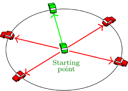
Figure 1: A wheeled robot follows a straight line from a known position with unknown heading. As perfect drives measure the relative displacement, any localization algorithm should “reflect” the car is on a circle centered on the initial position with known radius, and optimising over the entire state $(\theta,\mathbf{x})$ to account for GPS position measurements should boil down to optimising over heading $\theta$ only.

However, a simple numerical experiment where the vehicle moves along a line at a speed of $7m/s$ with known initial position and a $-3\pi/4$ wrong initial heading (with an initial covariance matrix $diag((3\pi/4)^{2},0,0)$) proves this is not the case for standard smoothing methods, see Figure 2. This is because the information about the length is not a hard constraint for the optimisation algorithm. Neither is it for IS, but the latter’s descent step based on the invariant filtering framework [6] inherently respects this information.

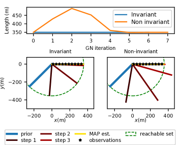
Figure 2: Conventional [24] and Invariant Smoothing [19] of the entire trajectory. Top: Trajectory length of successive iterations for both methods. Bottom: Estimated trajectories from the odometry, at the first descent steps, and at convergence. Both methods maintain a straight line, but only IS keeps a fixed and correct length at each descent step, being consistent with the uncertainty in the problem.

The remainder of this paper is devoted to the theoretical explanation of what is observed, and to the application of the results to the more challenging problem of inertial alignment.

III Lie group embeddings of the state space

We first briefly recall the invariant filtering framework [5, 6]. Owing to space limitation, we assume the reader has basic knowledge about Lie groups for robotics, and is referred to [1] for a general presentation. We consider a state $\raisebox{1.0pt}{$\boldsymbol{\chi}$}\in G$, a matrix Lie group of dimension $q$. Its Lie algebra $\mathfrak{g}$ is identified with ${\mathbb{R}}^{q}$. Thus we consider its exponential map to be defined as $\exp:{\mathbb{R}}^{q}\rightarrow G$. As it is locally invertible, we denote its inverse by $\log$. We recall the notion of adjoint operator matrix of $\raisebox{1.0pt}{$\boldsymbol{\chi}$}\in G$, $\mathbf{Ad}_{\raisebox{1.0pt}{$\boldsymbol{\chi}$}}$, which satisfy

$$\forall\raisebox{1.0pt}{$\boldsymbol{\chi}$}\in G,\boldsymbol{\xi}\in{\mathbb{R}}^{q},\ \raisebox{1.0pt}{$\boldsymbol{\chi}$}^{-1}\exp(\boldsymbol{\xi})\raisebox{1.0pt}{$\boldsymbol{\chi}$}=\exp(\mathbf{Ad}_{\raisebox{1.0pt}{$\boldsymbol{\chi}$}}\boldsymbol{\xi})$$ (2)

Group automorphisms are bijective maps $\Phi:G\rightarrow G$ satisfying $\Phi(\raisebox{1.0pt}{$\boldsymbol{\chi}$}\boldsymbol{\eta})=\Phi(\raisebox{1.0pt}{$\boldsymbol{\chi}$})\Phi(\boldsymbol{\eta})$ for $\raisebox{1.0pt}{$\boldsymbol{\chi}$},\boldsymbol{\eta}\in G$. The Lie group Lie algebra correspondance, see [9], ensures for any automorphism $\Phi$ there is $\mathbf{M}\in{\mathbb{R}}^{q\times q}$ so that

$$\forall(\raisebox{1.0pt}{$\boldsymbol{\chi}$},\boldsymbol{\xi})\in G\times{\mathbb{R}}^{q},\ \Phi(\raisebox{1.0pt}{$\boldsymbol{\chi}$}\exp(\boldsymbol{\xi}))=\Phi(\raisebox{1.0pt}{$\boldsymbol{\chi}$})\exp(\mathbf{M}\boldsymbol{\xi}),$$ (3)

see also the log-linearity property of [5]. The operator $\boldsymbol{\nu}\mapsto\raisebox{1.0pt}{$\boldsymbol{\chi}$}^{-1}\boldsymbol{\nu}\raisebox{1.0pt}{$\boldsymbol{\chi}$}$ is easily checked to be a group automorphism, and in this case we see from (2) that $\mathbf{M}=\mathbf{Ad}_{\raisebox{1.0pt}{$\boldsymbol{\chi}$}}$. We define random variables on Lie groups through the exponential, following [21, 12, 1, 13, 6]. The probability distribution $\raisebox{1.0pt}{$\boldsymbol{\chi}$}\sim\mathcal{N}_{L}(\bar{\raisebox{1.0pt}{$\boldsymbol{\chi}$}},\mathbf{P})$ for the random variable $\raisebox{1.0pt}{$\boldsymbol{\chi}$}\in G$ is defined as

$$\raisebox{1.0pt}{$\boldsymbol{\chi}$}=\bar{\raisebox{1.0pt}{$\boldsymbol{\chi}$}}\exp\left(\boldsymbol{\xi}\right),\text{~{}}\boldsymbol{\xi}\sim\mathcal{N}\left(\mathbf{0},\mathbf{P}\right),$$ (4)

In the following, we consider a discrete-time trajectory denoted as $(\raisebox{1.0pt}{$\boldsymbol{\chi}$}_{i})_{i}$ of the following system

$$\raisebox{1.0pt}{$\boldsymbol{\chi}$}_{0} \sim\mathcal{N}_{L}(\bar{\raisebox{1.0pt}{$\boldsymbol{\chi}$}},\mathbf{P}_{0}), \raisebox{1.0pt}{$\boldsymbol{\chi}$}_{i+1}=f_{i}(\raisebox{1.0pt}{$\boldsymbol{\chi}$}_{i})$$ (5a)

$$y_{k} =h_{k}(\raisebox{1.0pt}{$\boldsymbol{\chi}$}_{I_{k}})+\mathbf{n}_{k} \mathbf{n}_{k}\sim\mathcal{N}(0,\mathbf{N}_{k})$$ (5b)

where $f_{i}$ is the dynamics function, $\mathbf{P}_{0}\in{\mathbb{R}}^{q\times q}$ the initial state error covariance, $\mathbf{N}_{k}\in{\mathbb{R}}^{r\times r}$ the observation noise covariance, and $\raisebox{1.0pt}{$\boldsymbol{\chi}$}_{I_{k}}$ denotes a subset of the states which are involved in the measurements. Thus (5) reflects deterministic dynamics with noisy observations and uncertain initial state. Even if the framework of noise-free dynamics is unrealistic, it allows for a theory that studies how the smoother degenerates when noise tends to zero, as was already done in the context of Kalman filtering in [18, 10].

III-A Group-affine Dynamics

In the invariant framework, $f_{i}$ is assumed to be group affine. These dynamics were introduced in continuous time in [5], and in discrete time in [9]. The main idea is that they extend the notion of linear dynamics (i.e. defined by affine maps) from vector spaces to Lie groups.

Definition 1

Group affine dynamics are defined through

$$\raisebox{1.0pt}{$\boldsymbol{\chi}$}_{i+1}=f_{i}(\raisebox{1.0pt}{$\boldsymbol{\chi}$}_{i})=\boldsymbol{\Gamma}_{i}\Phi(\raisebox{1.0pt}{$\boldsymbol{\chi}$}_{i})\boldsymbol{\Upsilon}_{i}.$$ (6)

where $\boldsymbol{\Gamma}_{i},\boldsymbol{\Upsilon}_{i}\in G$, and $\Phi$ is an automorphism.

Group affine dynamics include a large class of systems of engineering interest revolving around navigation and robotics, as shown in e.g. [5, 9, 38, 33]. Note that, since $\boldsymbol{\nu}\mapsto\raisebox{1.0pt}{$\boldsymbol{\chi}$}^{-1}\boldsymbol{\nu}\raisebox{1.0pt}{$\boldsymbol{\chi}$}$ is a group automorphism, it is sufficient to define $f_{i}(\raisebox{1.0pt}{$\boldsymbol{\chi}$}_{i})=\Phi(\raisebox{1.0pt}{$\boldsymbol{\chi}$}_{i})\boldsymbol{\Upsilon}_{i}$. Both this and (6) prove equivalent, but the latter fits the equations of inertial navigation better [9, 13].

Group affine dynamics come with the log-linear property, originally introduced and proved in [5] and whose discrete-time counterpart is easier once (3) has been identified.

Proposition 1 (from [9], discrete-time log-linear property)

For group affine dynamics (6), we have

$$f_{i}(\raisebox{1.0pt}{$\boldsymbol{\chi}$}_{i}\exp(\boldsymbol{\xi}))=\raisebox{1.0pt}{$\boldsymbol{\chi}$}_{i+1}\exp(\mathbf{F}_{i}\boldsymbol{\xi})$$ (7)

with $\mathbf{F}_{i}=\bf\mathbf{Ad}_{\boldsymbol{\Upsilon}_{i}^{-1}}\mathbf{M}$ a linear operator, where $\mathbf{M}$ comes from (3).

Proof:

Focusing on, e.g., the first step, we have

$$\boldsymbol{\Gamma}_{0}\Phi(\raisebox{1.0pt}{$\boldsymbol{\chi}$}_{0}\exp(\boldsymbol{\xi}))\boldsymbol{\Upsilon}_{0} \stackrel{{\scriptstyle\eqref{eq:LGLA}}}{{=}}\boldsymbol{\Gamma}_{0}\Phi(\raisebox{1.0pt}{$\boldsymbol{\chi}$}_{0})\exp(\mathbf{M}\boldsymbol{\xi})\boldsymbol{\Upsilon}_{0}$$

$$\stackrel{{\scriptstyle\eqref{eq:adjoint}}}{{=}}\boldsymbol{\Gamma}_{0}\Phi(\raisebox{1.0pt}{$\boldsymbol{\chi}$}_{0})\boldsymbol{\Upsilon}_{0}\exp(\bf\mathbf{Ad}_{\boldsymbol{\Upsilon}_{0}^{-1}}\mathbf{M}\boldsymbol{\xi})$$

$$=\raisebox{1.0pt}{$\boldsymbol{\chi}$}_{1}\exp(\bf\mathbf{F}_{0}\boldsymbol{\xi}).$$ (8)

∎

III-B Lie group embedding for the introductory example

We insist that in the invariant filtering approach, Lie group embedding goes well beyond representing a state variable (e.g., using a rotation matrix to encode the vehicle’s orientation). It is more subtle, as various Lie group embeddings exist: Some bring properties and some do not. Back to the simple introductory example, the state and dynamics (1) should be embedded in the Lie group of 2D poses, $SE(2)$:

$$\raisebox{1.0pt}{$\boldsymbol{\chi}$}=\begin{bmatrix}\mathbf{R}(\theta)&\mathbf{x}\\ 0_{1\times 2}&1\end{bmatrix},\quad\raisebox{1.0pt}{$\boldsymbol{\chi}$}_{i+1}=\raisebox{1.0pt}{$\boldsymbol{\chi}$}_{i}\boldsymbol{\Upsilon}_{i},\quad\boldsymbol{\Upsilon}_{i}:=\begin{bmatrix}\mathbf{Id}&\mathbf{u}\\ 0_{1\times 2}&1\end{bmatrix}.$$ (9)

The dynamics obviously write as (6) with $\Phi(\raisebox{1.0pt}{$\boldsymbol{\chi}$}_{i})=\raisebox{1.0pt}{$\boldsymbol{\chi}$}_{i}$.

As initially the position is known to be $\bar{\mathbf{x}}_{0}$ the uncertainty entirely concerns $\theta$, and the initial state necessarily lies in the subpace $\{(\alpha,\bar{\mathbf{x}}_{0})|\alpha\in{\mathbb{R}}\}$ of the state space. In $SE(2)$ this translates into the initial state being of the form $\{\bar{\raisebox{1.0pt}{$\boldsymbol{\chi}$}}_{0}\exp(\alpha\boldsymbol{\xi}_{\theta}),\alpha\in{\mathbb{R}}\}$, where $\boldsymbol{\xi}_{\theta}=(0,0,1)^{T}$. In the formalism of (4), this translates into a rank 1 covariance matrix $\mathbf{P}_{0}$ whose range is spanned by $\boldsymbol{\xi}_{\theta}$.

III-C The Property of Reachability

The fact that the uncertainty is concentrated on a circle may be explained through the machinery of Lie groups in a more general setting as follows. Assume the initial state lies in a subspace of the state space defined by

$$\bar{\raisebox{1.0pt}{$\boldsymbol{\chi}$}}_{0}\exp(\sum_{j=1}^{p}\alpha_{j}\boldsymbol{\eta}_{j}),\quad(\alpha_{1},\cdots\alpha_{p})\in{\mathbb{R}}^{p}$$ (10)

with $\boldsymbol{\eta}_{1},\cdots,\boldsymbol{\eta}_{p}$ known vectors, and $p\leq q=\mathrm{dim}(G)$. The log-linear property, see (7), shows by induction that at timestep $i$ the state lies within a subspace of the state space of the same form

$$\bar{\raisebox{1.0pt}{$\boldsymbol{\chi}$}}_{i}\exp(\sum_{j=1}^{p}\alpha_{j}\widetilde{\mathbf{F}}_{i}\boldsymbol{\eta}_{j}),\qquad\widetilde{\mathbf{F}}_{i}=\mathbf{F}_{i-1}\ldots\mathbf{F}_{0}$$ (11)

Definition 2

For an initial state of the form (10) and noise-free group affine dynamics (6), the set of physically reachable states at timestep $i$ is defined as $\{\bar{\raisebox{1.0pt}{$\boldsymbol{\chi}$}}_{i}\exp\bigl{(}\sum_{j=1}^{p}\alpha_{j}\widetilde{\mathbf{F}}_{i}\boldsymbol{\eta}_{j}\bigr{)}|\alpha_{1},\cdots,\alpha_{p}\in{\mathbb{R}}\}$.

To embrace the framework of statistics - as smoothing algorithms aim at computing the most likely trajectory - we need to define uncertainty on the state space being consistent with the notion of reachability.

We define an initial belief on the state to be of the form (4) where the initial state’s covariance $\mathbf{P}_{0}$ is of rank $p<q$. Denoting by $\boldsymbol{\eta}_{1},\cdots,\boldsymbol{\eta}_{p}$ vectors of the Lie algebra that support $\mathbf{P}_{0}$, the initial distribution is then supported by a subspace of the form (10), and any estimator which is consistent with the probabilistic setting should return estimates lying within the set of reachable states.

For technical reasons, see [18, 10], we will systematically assume the vectors supporting the initial distribution form a Lie subalgebra: for all $i,j$ the vector $[\boldsymbol{\eta}_{i},\boldsymbol{\eta}_{j}]$, the Lie bracket of $\boldsymbol{\eta}_{i},\boldsymbol{\eta}_{j}$ [21, 1], is a linear combination of $\boldsymbol{\eta}_{1},\cdots,\boldsymbol{\eta}_{p}$.

Considered problem: To summarise, what we would like to do is to devise a smoothing algorithm, that is such that when the initial state distribution is of the form (4) where the initial state’s covariance $\mathbf{P}_{0}$ is of rank $p<q$, and the dynamics are noise-free and group-affine (6), the estimates $(\hat{}\raisebox{1.0pt}{$\boldsymbol{\chi}$}_{i})_{1\leq i\leq n}$ all lie within the reachable subset (11), and this at each (descent) step of the optimization procedure.

IV Main Result

In this section, we prove that Invariant Smoothing (IS) solves the problem above. By contrast standard smoothing algorithms do not, as shown by Figure 2.

IV-A Smoothing on Lie groups

We first briefly recall the Invariant Smoothing (IS) framework introduced in [19]. Departing from a system of the form (5a) with observations (5b), the goal of smoothing is to find

$$(\raisebox{1.0pt}{$\boldsymbol{\chi}$}_{i})_{i}^{*}=\operatorname*{argmax}_{(\raisebox{1.0pt}{$\boldsymbol{\chi}$}_{i})_{1\leq i\leq n}}\mathbb{P}((\raisebox{1.0pt}{$\boldsymbol{\chi}$}_{i})_{i}|y_{0},\dots,y_{n})$$ (12)

i.e., the maximum a posteriori (MAP) estimate of the trajectory. It is usually found through the Gauss-Newton algorithm. First we devise a cost function associated to Problem (12) as the negative log likelihood

$$\mathcal{C}=-\log\bigl{(}\mathbb{P}((\raisebox{1.0pt}{$\boldsymbol{\chi}$}_{i})_{1\leq i\leq n}|y_{0},\dots,y_{n})\bigr{)}$$

that we seek to minimize. Given a current guess of the trajectory’s states, $(\hat{\raisebox{1.0pt}{$\boldsymbol{\chi}$}}_{i})_{i}$, the cost function $\mathcal{C}$ is linearised and then the resulting linear problem is solved exactly, yielding a novel estimate, and so on until convergence. Since $\raisebox{1.0pt}{$\boldsymbol{\chi}$}_{i}$ belongs to a Lie group, linearisation in IS is carried out as

$$\forall 1\leq i\leq n\quad\raisebox{1.0pt}{$\boldsymbol{\chi}$}_{i}=\hat{\raisebox{1.0pt}{$\boldsymbol{\chi}$}}_{i}\exp(\boldsymbol{\xi}_{i}).$$ (13)

where $(\boldsymbol{\xi}_{i})_{i}$ are the searched parameters that minimize the linearized cost. When considering an invertible prior $\mathbf{P}_{0}$ and noisy dynamics with covariance matrices $\mathbf{Q}_{i}$, IS linearises the cost $\mathcal{C}$ as [19]

$$\tilde{\mathcal{C}}= \|\mathbf{p}_{0}+\boldsymbol{\xi}_{0}\|_{\widetilde{\mathbf{P}}_{0}}^{2}$$ (14)

$$+\sum_{i}\|\hat{\mathbf{a}}_{i}-\mathbf{F}_{i}\boldsymbol{\xi}_{i}+\boldsymbol{\xi}_{i+1}\|_{\mathbf{Q}_{i}}^{2}+\sum_{k}\|\hat{\mathbf{n}}_{k}+\mathbf{H}_{k}\boldsymbol{\Xi}\|_{\mathbf{N}_{k}}^{2}$$

where we used the notation $\|\mathbf{Z}\|_{\mathbf{P}}^{2}=\mathbf{Z}^{T}\mathbf{P}^{-1}\mathbf{Z}$, and where $\boldsymbol{\Xi}$ is the concatenation of $(\boldsymbol{\xi}_{i})_{i}$. (14) relies on the Baker-Campbell-Haussdorff formula [1] $\log(\exp(a)\exp(b))=BCH(a,b)$. $\widetilde{\mathbf{P}}_{0}=\mathbf{J}_{0}^{-1}\mathbf{P}_{0}\mathbf{J}_{0}^{-T}$, where $\mathbf{J}_{0}$ is the right Jacobian of the Lie group $G$ [1, 21], satisfying $BCH(\mathbf{p}_{0},\boldsymbol{\xi})=\mathbf{p}_{0}+\mathbf{J}_{0}\boldsymbol{\xi}+o(\|\boldsymbol{\xi}\|^{2})$, $\mathbf{p}_{0}=\log(\bar{\raisebox{1.0pt}{$\boldsymbol{\chi}$}}_{0}^{-1}\hat{\raisebox{1.0pt}{$\boldsymbol{\chi}$}}_{0})$ with a prior $\bar{\raisebox{1.0pt}{$\boldsymbol{\chi}$}}_{0}$, $\hat{\mathbf{a}}_{i}=\log(f_{i}(\hat{\raisebox{1.0pt}{$\boldsymbol{\chi}$}}_{i})^{-1}\hat{\raisebox{1.0pt}{$\boldsymbol{\chi}$}}_{i+1})$, $\hat{\mathbf{n}}_{k}=\mathbf{y}_{k}-h_{k}(\hat{\raisebox{1.0pt}{$\boldsymbol{\chi}$}}_{I_{k}})$, and $\mathbf{F}_{i},\mathbf{H}_{k}$ are the (Lie group) Jacobians of $f_{i}$ and $h_{k}$ respectively. $\mathbf{H}_{k}$ was padded with zero blocks for the indices not contained in $I_{k}$. The principle of smoothing algorithms is to solve the linearized problem (14) in closed form, and to update the trajectory substituting the optimal $\boldsymbol{\xi}_{i}$ in (13). The problem is then relinearised at this new estimate until convergence.

IV-B Smoothing with no process noise and degenerate prior

However, in this paper we assumed the dynamics (5a) to be noise-free, that is, $\mathbf{Q}_{i}=0$, and $\mathbf{P}_{0}$ to be rank-deficient. As a result, the standard formulation (14) appears ill-defined. Moreover, when process noise is low this makes the normal equations solving it ill-conditioned. Theoretically, it turns out that a) (14) has a well-defined solution when $\mathbf{Q}_{i}\to 0$ and b) it is possible to solve (14) while avoiding matrix inversions, see [20]. In the present paper, this is none of our concern, and we assume a solver, e.g., [20], is able to flawlessly solve (14) for arbitrarily small process noise, even in the limiting case where $\mathbf{Q}_{i}\to 0$ and $\mathbf{P}_{0}$ is rank-deficient. Our concern is to study the consequences of this limiting case on the state updates. This provides insight in turn into the good behavior of the algorihtm in the presence of low process noise, as occurs in some applications like inertial navigation.

IV-C Main Result

Assuming (14) may be properly solved, even in the case of no process noise and rank-deficient $\mathbf{P}_{0}$, we show now that the batch Invariant Smoother yields estimates which are consistent with the physics of the problem (in other words the assumed uncertainty) at each descent step.

Theorem 1

Consider the system described by noise-free dynamics (5a) assumed to be group affine. Let $(\hat{\raisebox{1.0pt}{$\boldsymbol{\chi}$}}_{i})_{i}$ represent the current estimates of an Invariant Smoother [19]. Then every iteration of the optimization algorithms exhibits the two following properties (if initalised accordingly):

1. Limiting equality constraints. Equality constraints induced by noise-free dynamics are seamlessly handled by the unconstrained optimization algorithm, which is such that at all steps we have $\hat{\raisebox{1.0pt}{$\boldsymbol{\chi}$}}_{i+1}=f_{i}(\hat{\raisebox{1.0pt}{$\boldsymbol{\chi}$}}_{i})$.

2. Belief-compatible estimates. Assume the prior about the initial state is such that $\mathbf{P}_{0}$ in (5a) is supported by a vector space $\mathbf{V}_{0}$ of dimension $p<q$, spanned by, say, $\boldsymbol{\eta}_{0},\ldots,\boldsymbol{\eta}_{p}$, and such that for all $i,j$, $[\boldsymbol{\eta}_{i},\boldsymbol{\eta}_{j}]\in\mathbf{V}_{0}$: all iterations of the algorithm are in the reachable subspace.

Proof:

We detail the proof of the theorem for a simplified case, where only two states are considered, i.e. one propagation step. Consider the estimates of a two states trajectory $(\hat{\raisebox{1.0pt}{$\boldsymbol{\chi}$}}_{0},\hat{\raisebox{1.0pt}{$\boldsymbol{\chi}$}}_{1})$, where $\hat{\raisebox{1.0pt}{$\boldsymbol{\chi}$}}_{0}$ is reachable, and satisfying $\hat{\raisebox{1.0pt}{$\boldsymbol{\chi}$}}_{1}=f_{0}(\hat{\raisebox{1.0pt}{$\boldsymbol{\chi}$}}_{0})$. After the next IS update, they will become $(\hat{\raisebox{1.0pt}{$\boldsymbol{\chi}$}}_{0}\exp(\boldsymbol{\xi}_{0}^{*}),\hat{\raisebox{1.0pt}{$\boldsymbol{\chi}$}}_{1}\exp(\boldsymbol{\xi}_{1}^{*}))$ where a linear solver returns the solutions $\boldsymbol{\xi}_{0}^{*},\boldsymbol{\xi}_{1}^{*}$ to (14) in the considered degenerate case. We want to prove

1. $\hat{\raisebox{1.0pt}{$\boldsymbol{\chi}$}}_{1}\exp(\boldsymbol{\xi}_{1}^{*})=f_{0}(\hat{\raisebox{1.0pt}{$\boldsymbol{\chi}$}}_{0}\exp(\boldsymbol{\xi}_{0}^{*}))$,

2. if $\hat{\raisebox{1.0pt}{$\boldsymbol{\chi}$}}_{0},\hat{\raisebox{1.0pt}{$\boldsymbol{\chi}$}}_{1}$ lie in their respective reachable subspaces, so do $\hat{\raisebox{1.0pt}{$\boldsymbol{\chi}$}}_{0}\exp(\boldsymbol{\xi}_{0}^{*}),\hat{\raisebox{1.0pt}{$\boldsymbol{\chi}$}}_{1}\exp(\boldsymbol{\xi}_{1}^{*})$.

To do so we start proving IS is such that in the present case

$$\boldsymbol{\xi}_{1}^{*} =\mathbf{F}_{0}\boldsymbol{\xi}_{0}^{*}$$ (15)

$$\boldsymbol{\xi}_{0}^{*} \in\mathbf{V}_{0}$$ (16)

(15) implies (i) from the log-linear property (7). As $\hat{\raisebox{1.0pt}{$\boldsymbol{\chi}$}}_{0}$ is in the reachable subspace, and as $\mathbf{V}_{0}$ forms a Lie subalgebra (hence the technical assumption of stability by Lie bracket), we see (16) implies (ii) as concerns $\boldsymbol{\xi}_{0}^{*}$ and the similar property regarding $\boldsymbol{\xi}_{1}^{*}$ will immediately stem from (15). As the remainder of the proof is more technical and less insightful, and requires results from [20], it has been moved to the appendix.

∎

Note, first, that this theorem holds for any solver capable of handling $\mathbf{Q}_{i}=\mathbf{0}$ and rank-deficient $\mathbf{P}_{0}$. Moreover, it is stronger than just saying all states are individually reachable. Here, they all share the same $(\alpha_{j})_{1\leq j\leq p}$ from (11). Finally, it underlies the results observed in Figure 2: The fact each iteration appears to be a possible trajectory of the noise-free dynamics (1) stems from (i), that is, each trajectory intermediate estimate is a straight line with correct length, by contrast to the the standard smoother that distorts the trajectory at each optimization step. The fact all estimates belong to circles that are compatible with the initial belief encoded in the covariance matrix $diag((3\pi/4)^{2},0,0)$ stems from (ii).

V Application to INS Alignment

In “genuine” Inertial Navigation Systems (INS), an initialisation process that relates the body frame to the world frame is required, and this process is called alignment, see e.g., [41, 22, 27, 17]. This is a challenging process that takes time as the orientation of the carrier is difficult to estimate (the vertical is rapidly found as it is sensed by the accelerometers, but the geographic North is much more difficult to observe). As a result, the main uncertainty during the whole process is dispersed almost exclusively around the vertical axis but it may be very large since the use of magnetometers is generally banned (they are too imprecise and too sensitive to metallic and electromagnetic materials around). Of course alignment is afforded only by highly precise gyrometers, which justifies the use of a very low noise.

We consider herein low-noise and unbiased inertial sensors, to illustrate the practical implications of the noise-free results. We also show the advantage of IS over state-of-the-art smoothing methods for inertial navigation [25, 23].

V-A Lie Group Embedding

Important discoveries of [5] are the group-affine property and the introduction of $SE_{2}(3)$ as a Lie group embedding which makes navigation equations group-affine.

V-A1 Unbiased inertial navigation is group affine

Consider a robot equipped with an IMU. For unbiased navigation, the state consists of the attitude be $\mathbf{R}$, velocity $\mathbf{v}$ and position $\mathbf{x}$. Unbiased inertial navigation’s dynamics are given by

$$f_{\boldsymbol{\omega},\mathbf{a}}\begin{pmatrix}\mathbf{R}\\ \mathbf{v}\\ \mathbf{x}\end{pmatrix}=\left\{\begin{matrix}\mathbf{R}\exp_{SO(3)}(dt(\boldsymbol{\omega}+\mathbf{w}_{g}))\\ \mathbf{v}+dt(\mathbf{R}(\mathbf{a}+\mathbf{w}_{a})+\mathbf{g})\\ \mathbf{x}+dt\ \mathbf{v}\end{matrix}\right.$$ (17)

with $\boldsymbol{\omega},\mathbf{a}\in\mathbb{R}^{3}$ the gyrometers and accelerometers signals respectively, $\mathbf{w}_{g},\mathbf{w}_{a}$ the associated white noises, and $\mathbf{g}$ be the gravity vector.

Following [5], the set of navigation triplets $(\mathbf{R},\mathbf{v},\mathbf{x})$ can be endowed with a matrix Lie group structure, called $SE_{2}(3)$, and referred to as the group of double direct spatial isometries [5] or extended poses [13], through

$$SE_{2}(3):=\left\{\mathbf{T}=\begin{bmatrix}\begin{array}[]{ccc}\mathbf{R}&\mathbf{v}&\mathbf{x}\\ \mathbf{0}_{3\times 2}&\lx@intercol\hfil\mathbf{I}_{2}\hfil\lx@intercol\end{array}\end{bmatrix}\in{\mathbb{R}}^{5\times 5}\Bigg{|}\begin{matrix}\mathbf{R}\in SO(3)\\ \mathbf{v}\in{\mathbb{R}}^{3}\\ \mathbf{p}\in{\mathbb{R}}^{3}\end{matrix}\right\}.$$

In this setting, (17), defines group affine dynamics (see [13])

$$\boldsymbol{\Gamma}_{i}= \begin{bmatrix}\begin{array}[]{ccc}\mathbf{Id}&dt\mathbf{g}&\mathbf{0}\\ \mathbf{0}_{3\times 2}&\lx@intercol\hfil\mathbf{I}_{2}\hfil\lx@intercol\end{array}\end{bmatrix},~{}\Phi(\mathbf{T})=\begin{bmatrix}\begin{array}[]{ccc}\mathbf{R}&\mathbf{v}&\mathbf{x}+dt\mathbf{v}\\ \mathbf{0}_{3\times 2}&\lx@intercol\hfil\mathbf{I}_{2}\hfil\lx@intercol\end{array}\end{bmatrix}$$

$$\boldsymbol{\Upsilon}_{i} =\begin{bmatrix}\begin{array}[]{ccc}\exp_{SO(3)}(dt\boldsymbol{\omega})&dt\mathbf{a}_{i}&\mathbf{0}\\ \mathbf{0}_{3\times 2}&\lx@intercol\hfil\mathbf{I}_{2}\hfil\lx@intercol\end{array}\end{bmatrix}$$ (18)

Let us illustrate how the propagation factors of IS are obtained. Let the residual be $\log(f_{i}(\raisebox{1.0pt}{$\boldsymbol{\chi}$}_{i})^{-1}\raisebox{1.0pt}{$\boldsymbol{\chi}$}_{i+1})=\log(\mathbf{\Delta_{IMU})}$. The Jacobian is computed with (6) and (13):

$$\mathbf{\Delta}_{IMU} =\boldsymbol{\Upsilon}_{i}^{-1}\Phi(\exp(-\boldsymbol{\xi}_{i})\hat{\raisebox{1.0pt}{$\boldsymbol{\chi}$}}_{i}^{-1})\boldsymbol{\Gamma}_{i}^{-1}\hat{\raisebox{1.0pt}{$\boldsymbol{\chi}$}}_{i+1}\exp(\boldsymbol{\xi}_{i+1})$$ (19)

$$=\exp(-\mathbf{F}_{i}\boldsymbol{\xi}_{i})f_{i}(\hat{\raisebox{1.0pt}{$\boldsymbol{\chi}$}}_{i})^{-1}\hat{\raisebox{1.0pt}{$\boldsymbol{\chi}$}}_{i+1}\exp(\boldsymbol{\xi}_{i+1})$$ (20)

$$\log(\mathbf{\Delta} {}_{IMU})\approx-\mathbf{F}_{i}\boldsymbol{\xi}_{i}+\boldsymbol{\xi}_{i+1}+\log(f_{i}(\hat{\raisebox{1.0pt}{$\boldsymbol{\chi}$}}_{i})^{-1}\hat{\raisebox{1.0pt}{$\boldsymbol{\chi}$}}_{i+1}),$$ (21)

where $\mathbf{F}_{i}=\mathbf{Ad}_{\boldsymbol{\Upsilon}_{i}^{-1}}\mathbf{M}$, which are given on $SE_{2}(3)$ by

$${\scriptstyle\mathbf{Ad_{\mathbf{T}}}=\begin{bmatrix}\mathbf{R}&\mathbf{0}_{3\times 3}&\mathbf{0}_{3\times 3}\\ \mathbf{v}_{\times}\mathbf{R}&\mathbf{R}&\mathbf{0}_{3\times 3}\\ \mathbf{p}_{\times}\mathbf{R}&\mathbf{0}_{3\times 3}&\mathbf{R}\end{bmatrix}\quad\mathbf{M}=\begin{bmatrix}\mathbf{I}_{3}&\mathbf{0}_{3\times 3}&\mathbf{0}_{3\times 3}\\ \mathbf{0}_{3\times 3}&\mathbf{I}_{3}&\mathbf{0}_{3\times 3}\\ \mathbf{0}_{3\times 3}&dt\mathbf{I}_{3}&\mathbf{I}_{3}\end{bmatrix}.}$$

V-A2 Uncertainty propagation

On $SE_{2}(3)$, the true IMU measurement $\tilde{\boldsymbol{\Upsilon}}$ can be related to the noisy ones $\boldsymbol{\Upsilon}$ through $\tilde{\boldsymbol{\Upsilon}}=\boldsymbol{\Upsilon}\exp(\mathbf{w})$, where $\mathbf{w}$ is a white noise on ${\mathbb{R}}^{9}$ and $\exp$ denotes the exponential map of $SE_{2}(3)$. For more on $SE_{2}(3)$, and its use for inertial navigation (notably the derivation of the covariance process noise matrix) the reader is referred to [5, 13].

V-B Difference between IS and other Smoothers

Let us compare IS with the state-of-the-art smoothing methods for inertial data [25], and the one implemented in GTSAM [23] (which slightly differs). The considered residuals are essentially the same, and so are their covariances, although obtained through less tedious computations. The main difference lies in the parametrisation of the state (i.e. the retraction) used to update the state variables at each optimization descent step. Indeed, the retractions used in [25] and GTSAM [23] are respectively

$$(\hat{\mathbf{R}},\hat{\mathbf{v}},\hat{\mathbf{x}}) \leftarrow(\hat{\mathbf{R}}\boldsymbol{\delta}_{R},\hat{\mathbf{v}}+\boldsymbol{\delta}_{v},\hat{\mathbf{x}}+\hat{\mathbf{R}}\boldsymbol{\delta}_{x}),$$ (22)

$$(\hat{\mathbf{R}},\hat{\mathbf{v}},\hat{\mathbf{x}}) \leftarrow(\hat{\mathbf{R}}\boldsymbol{\delta}_{R},\hat{\mathbf{v}}+\hat{\mathbf{R}}\boldsymbol{\delta}_{v},\hat{\mathbf{x}}+\hat{\mathbf{R}}\boldsymbol{\delta}_{x}).$$ (23)

which are linear by nature whereas the exponential map offers a fully nonlinear appropriate map. Note that (23) is a first-order approximation of the Lie exponential on $SE_{2}(3)$. Jacobians for (23) can be retrived from (19), as

$$\mathbf{\Delta}_{IMU} =f_{i}(\hat{\raisebox{1.0pt}{$\boldsymbol{\chi}$}}_{i})^{-1}\hat{\raisebox{1.0pt}{$\boldsymbol{\chi}$}}_{i+1}\exp(-\hat{\mathbf{F}}_{i}\boldsymbol{\xi}_{i})\exp(\boldsymbol{\xi}_{i+1}),$$ (24)

where $\hat{\mathbf{F}}_{i}=\mathbf{Ad}_{\hat{\boldsymbol{\Upsilon}}_{i}^{-1}}\mathbf{M}$ is the wanted Jacobian, with $\hat{\boldsymbol{\Upsilon}}_{i}=\Phi(\hat{\raisebox{1.0pt}{$\boldsymbol{\chi}$}}_{i})^{-1}\boldsymbol{\Gamma}_{i}^{-1}\hat{\raisebox{1.0pt}{$\boldsymbol{\chi}$}}_{i+1}$ representing the “estimated” measurement. Jacobian for (22) can then be easily derived. The other difference is that IS uses the logartihm map of $SE_{2}(3)$.

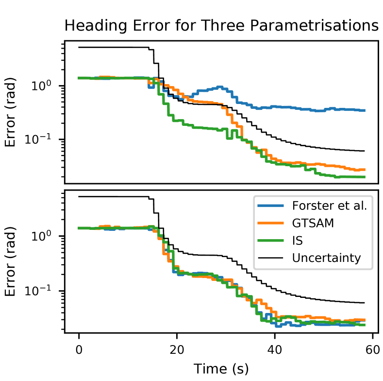
Figure 3: Yaw error (on a log scale) for the alignment problem of Section V, starting with initial heading error of 80^∘ over time. IS is compared with [25] and GTSAM [23]. “Uncertainty” denotes the $3\sigma$ envelope of the IS estimate. Top: sliding window of size 10. Bottom: sliding window of size 50.

V-C Experimental Setting

We compare the three smoothing methods on a simulated in-motion alignment problem. A vehicle is equipped with a precise IMU and a GPS sensor. The IMU and GPS measurements are acquired at 200 Hz and 1 Hz respectively, and considered with the following standard deviations

$$\sigma_{g}=2.7e-4~{}^{\circ}/s,~{}\sigma_{a}=1.5e-3m/s^{2},~{}\sigma_{n}=3m$$ (25)

The initial position is supposed to be known, as is customary for initial alignment, but with unknown speed and attitude:

$$\sigma_{p}^{0}=0m,\sigma_{v}^{0}=10m/s,\sigma_{R}^{0}=100~{}^{\circ}$$ (26)

The trajectory starts with the vehicle standing still for 15s, before starting to move forward for 25s. The estimate is initialised with zero velocity, correct roll and pitch, and an incorrect heading of 80^∘, as it may be assumed that roll and pitch are rapidly identified, as they are highly observable. The IMU is preintegrated between each GPS measurements, see [25, 7], where updates occur. The estimation was carried out in a sliding window setting, where the oldest state is marginalised out once the maximum of states is reached. Two experiments were carried out, with windows of size 10 and 50, so that in the first one marginalisation starts before the yaw has converged. One Gauss-Newton iteration is carried out at each update.

V-D Results

The results are displayed on Figure 3. Although the whole navigation state is estimated, only the yaw error is reported, as it is the key parameter which is difficult to estimate. The RMSE is computed over 10 Monte Carlo runs. The $3\sigma$ bound of the yaw estimate of IS is also reported (the bounds of both other methods are very similar). In the top chart, which involves a sliding window of 10 time steps, we see that [25] (Forster et al.) becomes inconsistent due to early marginalisation. As concerns the two other algorithms, IS and GTSAM [23] both coincide after convergence indeed, but IS shows quicker convergence and better consistency since GTSAM exceeds the $3\sigma$ bound between 20 and 30 seconds. This is due to the fact that GTSAM uses $\hat{\boldsymbol{\Upsilon}}_{i}$, which becomes erroneous after update (23), even with $\mathbf{Q}_{i}=\mathbf{0}$. In the case of a sliding window of size 50 (bottom chart), [25] converges to the IS and GTSAM estimates, since they share the same cost function. Indeed, the vehicle starts moving before marginalisation occurs, so less errors are propagated, ensuring better estimators’ consistency.

VI Conclusion

This paper first presented a new theoretical property of the recently introduced Invariant Smoothing (IS) framework, which was shown to respect a class of geometrical constraints appearing in the limit-case of noise-free dynamics, advocating for its use in high-accuracy navigation. This was illustrated by a 2D introductory wheeled robot localisation simulated problem, for which only IS managed to produce consistent successive iterations. The impact of this result for unbiased inertial navigation, with low but non-null process noise, was then evaluated on alignment simulations using a high-grade IMU. In this case, IS proved more stable and consistent than state-of-the-art inertial smoothing methods. Future work will further study the impact of the window size on smoothing methods, and how this adapts to biased inertial navigation, using the recently introduced two-frames group [8] providing a novel embedding that better accommodates sensor biases.

We now complete the proof of the theorem. We first recall results of [20]. As concerns (14), it may be re-written as

$$\begin{bmatrix}\boldsymbol{\xi}_{0}^{*}\\ \boldsymbol{\xi}_{1}^{*}\end{bmatrix}=\operatorname*{argmin}_{\boldsymbol{\xi}_{0},\boldsymbol{\xi}_{1}}\left\|\mathbf{A}_{0}\begin{bmatrix}\boldsymbol{\xi}_{0}\\ \boldsymbol{\xi}_{1}\end{bmatrix}-\mathbf{b}_{0}\right\|_{\boldsymbol{\Pi}_{0}}^{2}+\left\|\mathbf{H}_{1}\begin{bmatrix}\boldsymbol{\xi}_{0}\\ \boldsymbol{\xi}_{1}\end{bmatrix}-\hat{\mathbf{n}}_{1}\right\|_{\mathbf{N}_{1}}^{2},$$ (27)

where $\mathbf{A}_{0}=\begin{bmatrix}\mathbf{Id}\\ -\mathbf{F}_{0}&\mathbf{Id}\end{bmatrix}$, $\mathbf{b}_{0}=\begin{bmatrix}\mathbf{p}_{0}\\ \hat{\mathbf{a}}_{0}\end{bmatrix}$, $\boldsymbol{\Pi}_{0}=\text{diag}(\widetilde{\mathbf{P}}_{0},\mathbf{Q}_{0})$ defined in (14). This yields a solution to (27) as (see [20])

$$\begin{bmatrix}\boldsymbol{\xi}_{0}^{*}\\ \boldsymbol{\xi}_{1}^{*}\end{bmatrix} =\mathbf{A}_{0}^{-1}\left(\left(\mathbf{Id}-\mathbf{K}\mathbf{L}\right)\mathbf{b}_{0}+\mathbf{K}\hat{\mathbf{n}}_{1}\right)$$ (28a)

$$\mathbf{L}=\mathbf{H}_{1}\mathbf{A}_{0}^{-1} \qquad\mathbf{K}=\boldsymbol{\Pi}_{0}\mathbf{L}^{T}(\mathbf{L}\boldsymbol{\Pi}_{0}\mathbf{L}^{T}+\mathbf{N}_{1})^{-1}$$ (28b)

By assumption, $\mathbf{Q}_{0}=\mathbf{0}$ and $\hat{\mathbf{a}}_{0}=\log(f_{0}(\hat{\raisebox{1.0pt}{$\boldsymbol{\chi}$}}_{0})^{-1}\hat{\raisebox{1.0pt}{$\boldsymbol{\chi}$}}_{1})=\mathbf{0}$. Note that (28) provides a solver accomodating $\mathbf{Q}_{0}=\mathbf{0}$ and rank-deficient $\mathbf{P}_{0}$, as mentioned in Section IV-B. Let $\mathbf{L}=\begin{bmatrix}\mathbf{L}_{0}&\mathbf{L}_{1}\end{bmatrix}$, we then have

$$\mathbf{K}=\begin{bmatrix}\widetilde{\mathbf{P}}_{0}\\ &\mathbf{0}\end{bmatrix}\begin{bmatrix}\mathbf{L}_{0}^{T}\\ \mathbf{L}_{1}^{T}\end{bmatrix}\underbrace{(\mathbf{L}\boldsymbol{\Pi}_{0}\mathbf{L}^{T}+\mathbf{N}_{1})^{-1}}_{\boldsymbol{\Sigma}}=\begin{bmatrix}\widetilde{\mathbf{P}}_{0}\mathbf{L}_{0}^{T}\boldsymbol{\Sigma}\\ \mathbf{0}\end{bmatrix}$$

$$\begin{bmatrix}\boldsymbol{\xi}_{0}^{*}\\ \boldsymbol{\xi}_{1}^{*}\end{bmatrix}=\begin{bmatrix}\mathbf{Id}\\ \mathbf{F}_{0}&\mathbf{Id}\end{bmatrix}\begin{bmatrix}\mathbf{p}_{0}+\widetilde{\mathbf{P}}_{0}\mathbf{L}_{0}^{T}\boldsymbol{\Sigma}(\hat{\mathbf{n}}_{1}-\mathbf{L}_{0}\mathbf{p}_{0})\\ \mathbf{0}\end{bmatrix}$$ (29)

Recall that $\widetilde{\mathbf{P}}_{0}=\mathbf{J}_{0}^{-1}\mathbf{P}_{0}\mathbf{J}_{0}^{-T}$ from (14). By assumption, $\mathbf{p}_{0}=\log(\bar{\raisebox{1.0pt}{$\boldsymbol{\chi}$}}_{0}^{-1}\hat{\raisebox{1.0pt}{$\boldsymbol{\chi}$}}_{0})\in\mathbf{V}_{0}$ and $\mathbf{V}_{0}$ is a Lie subalgebra, so for any $\mathbf{e}\in\mathbf{V}_{0}$, $\mathbf{J}_{0}^{-1}\mathbf{e}\in\mathbf{V}_{0}$ [1]. Since $\mathbf{P}_{0}$ is spanned by $\boldsymbol{\eta}_{1},\ldots,\boldsymbol{\eta}_{p}\in\mathbf{V}_{0}$, then it has its image in $\mathbf{V}_{0}$, and so does $\widetilde{\mathbf{P}}_{0}$. $\mathbf{V}_{0}$ being closed by addition, this shows that $\boldsymbol{\xi}_{0}^{*}\in\mathbf{V}_{0}$. Moreover, it is straightforward that $\boldsymbol{\xi}_{1}^{*}=\mathbf{F}_{0}\boldsymbol{\xi}_{0}^{*}$. For longer trajectories, the proof easily generalises, as the involved matrices keep the same structure: $\mathbf{K}$ and $\mathbf{b}_{0}$ only have a non-zero first block row, and the first column of $\mathbf{A}_{0}^{-1}$ contains the $\widetilde{\mathbf{F}}_{i}$ from (11).

References

- [1] Timothy D. Barfoot. State Estimation for Robotics. Cambridge University Press, 2017.
- [2] Axel Barrau. Non-linear state error based extended Kalman filters with applications to navigation. PhD thesis, Mines Paristech, 2015.
- [3] Axel Barrau and Silvere Bonnabel. Alignment method for an inertial unit. French patent FR1302705A, worldwide WO2015075248A1, 2013.
- [4] Axel Barrau and Silvère Bonnabel. An EKF-SLAM algorithm with consistency properties. CoRR, abs/1510.06263, 2015.
- [5] Axel Barrau and Silvère Bonnabel. The invariant extended kalman filter as a stable observer. IEEE Transactions on Automatic Control, 62(4):1797–1812, April 2017.
- [6] Axel Barrau and Silvère Bonnabel. Invariant kalman filtering. Annual Review of Control, Robotics, and Autonomous Systems, 1(1):null, 2018.
- [7] Axel Barrau and Silvère Bonnabel. A mathematical framework for imu error propagation with applications to preintegration. In IEEE International Conference on Robotics and Automation (ICRA), 2020.
- [8] Axel Barrau and Silvere Bonnabel. The geometry of navigation problems. IEEE Transactions on Automatic Control, pages 1–1, 2022.
- [9] Axel Barrau and Silvère Bonnabel. Linear observed systems on groups. Systems and Control Letters, 129:36 – 42, 2019.
- [10] Axel Barrau and Silvère Bonnabel. Extended kalman filtering with nonlinear equality constraints: A geometric approach. IEEE Transactions on Automatic Control, 65(6):2325–2338, 2020.
- [11] Silvère Bonnabel, Philippe Martin, and Erwan Salaün. Invariant extended Kalman filter: theory and application to a velocity-aided attitude estimation problem. In Decision and Control, 2009 held jointly with the 2009 28th Chinese Control Conference. CDC/CCC 2009. Proceedings of the 48th IEEE Conference on, pages 1297–1304. IEEE, 2009.
- [12] Guillaume Bourmaud, Rémi Mégret, Audrey Giremus, and Yannick Berthoumieu. Discrete extended Kalman filter on Lie groups. In Signal Processing Conference (EUSIPCO), 2013 Proceedings of the 21st European, pages 1–5. IEEE, 2013.
- [13] Martin Brossard, Axel Barrau, Paul Chauchat, and Silvére Bonnabel. Associating uncertainty to extended poses for on lie group imu preintegration with rotating earth. IEEE Transactions on Robotics, pages 1–18, 2021.
- [14] D. Caruso, A. Eudes, M. Sanfourche, D. Vissière, and G. L. Besnerais. Magneto-visual-inertial dead-reckoning: Improving estimation consistency by invariance. In 2019 IEEE 58th Conference on Decision and Control (CDC), pages 7923–7930, 2019.
- [15] Jaehyuck Cha, Jeong Ho Hwang, and Chan Gook Park. Effect of adaptive fading scheme on invariant ekf for initial alignment under large attitude error and wave disturbance condition. In 2021 21st International Conference on Control, Automation and Systems (ICCAS), pages 477–480. IEEE, 2021.
- [16] Lubin Chang, Jingbo Di, and Fangjun Qin. Inertial based integration with transformed ins mechanization in earth frame. IEEE/ASME Transactions on Mechatronics, 2021.
- [17] Lubin Chang, Fangjun Qin, and Jiangning Xu. Strapdown inertial navigation system initial alignment based on group of double direct spatial isometries. IEEE Sensors Journal, 22(1):803–818, 2021.
- [18] P. Chauchat, A. Barrau, and S. Bonnabel. Kalman filtering with a class of geometric state equality constraints. In 2017 IEEE 56th Annual Conference on Decision and Control (CDC), pages 2581–2586, Dec 2017.
- [19] Paul Chauchat, Axel Barrau, and Silvere Bonnabel. Invariant Smoothing on Lie Groups. In IEEE/RSJ International Conference on Intelligent Robots and Systems, IROS 2018, Madrid, Spain, October 2018.
- [20] Paul Chauchat, Axel Barrau, and Silvère Bonnabel. Factor graph-based smoothing without matrix inversion for highly precise localization. IEEE Transactions on Control Systems Technology, 29(3):1219–1232, 2021.
- [21] Gregory S Chirikjian. Stochastic Models, Information Theory, and Lie Groups, Volume 2: Analytic Methods and Modern Applications. Springer Science & Business Media, 2011.
- [22] Xiao Cui, Chunbo Mei, Yongyuan Qin, Gongmin Yan, and Qiangwen Fu. In-motion alignment for low-cost sins/gps under random misalignment angles. Journal of Navigation, 70(6):1224–1240, 2017.
- [23] Franck Dellaert. Factor graphs and GTSAM: A hands-on introduction. Technical report, Georgia Institute of Technology, 2012.
- [24] Frank Dellaert and Michael Kaess. Square root sam: Simultaneous localization and mapping via square root information smoothing. The International Journal of Robotics Research, 25(12):1181–1203, 2006.
- [25] Christian Forster, Luca Carlone, Frank Dellaert, and Davide Scaramuzza. On-manifold preintegration for real-time visual–inertial odometry. IEEE Transactions on Robotics, 33(1):1–21, Feb 2017.
- [26] Christian Forster, Zichao Zhang, Michael Gassner, Manuel Werlberger, and Davide Scaramuzza. Svo: Semidirect visual odometry for monocular and multicamera systems. IEEE Transactions on Robotics, 33(2):249–265, April 2017.
- [27] Hongpo Fu, Yongmei Cheng, and Tianyi Zhang. A new invariant extended kalman filter based initial alignment method of sins under large misalignment angle. In 2021 China Automation Congress (CAC), pages 57–62. IEEE, 2021.
- [28] Ross Hartley, Maani Ghaffari Jadidi, Jessy Grizzle, and Ryan M Eustice. Contact-aided invariant extended kalman filtering for legged robot state estimation. In Proceedings of Robotics: Science and Systems, Pittsburgh, Pennsylvania, June 2018.
- [29] S. Heo and C. G. Park. Consistent ekf-based visual-inertial odometry on matrix lie group. IEEE Sensors Journal, 18(9):3780–3788, May 2018.
- [30] Minh-Duc Hua, Guillaume Ducard, Tarek Hamel, Robert Mahony, and Konrad Rudin. Implementation of a nonlinear attitude estimator for aerial robotic vehicles. Control Systems Technology, IEEE Transactions on, 22(1):201–213, 2014.
- [31] V. Indelman, S. Williams, Michael Kaess, and F. Dellaert. Information fusion in navigation systems via factor graph based incremental smoothing. Journal of Robotics and Autonomous Systems, RAS, 61(8):721–738, August 2013.
- [32] Michael Kaess, Hordur Johannsson, Richard Roberts, Viorela Ila, John J. Leonard, and Frank Dellaert. iSAM2: Incremental smoothing and mapping using the Bayes tree. The International Journal of Robotics Research, 31:217–236, 2012.
- [33] Robert E. Mahony and Tarek Hamel. A geometric nonlinear observer for simultaneous localisation and mapping. In 56th IEEE Annual Conference on Decision and Control, CDC 2017, Melbourne, Australia, December 12-15, 2017, pages 2408–2415, 2017.
- [34] Wei Ouyang and Yuanxin Wu. Optimization-based strapdown attitude alignment for high-accuracy systems: Covariance analysis with applications. IEEE Transactions on Aerospace and Electronic Systems, 2022.
- [35] T. Pfeifer and P. Protzel. Expectation-maximization for adaptive mixture models in graph optimization. In 2019 IEEE International Conference on Robotics and Automation (ICRA), 2019.
- [36] RM Eustice R Hartley, M Ghaffari and JW Grizzle. Contact-aided invariant extended kalman filtering for robot state estimation. In The International Journal of Robotics Research, 2019.
- [37] Niels van Der Laan, Mitchell Cohen, Jonathan Arsenault, and James Richard Forbes. The invariant rauch-tung-striebel smoother. IEEE Robotics and Automation Letters, 5(4):5067–5074, 2020.
- [38] A. Walsh, J. Arsenault, and J. R. Forbes. Invariant sliding window filtering for attitude and bias estimation. In 2019 American Control Conference (ACC), pages 3161–3166, July 2019.
- [39] Kevin C. Wolfe, Michael Mashner, and Gregory S. Chirikjian. Bayesian fusion on Lie groups. Journal of Algebraic Statistics, 2(1):75–97, 2011.
- [40] K. Wu, T. Zhang, D. Su, S. Huang, and G. Dissanayake. An invariant-ekf vins algorithm for improving consistency. In 2017 IEEE/RSJ International Conference on Intelligent Robots and Systems (IROS), pages 1578–1585, Sep. 2017.
- [41] Yuanxin Wu and Xianfei Pan. Velocity/position integration formula part i: Application to in-flight coarse alignment. IEEE Transactions on Aerospace and Electronic Systems, 49(2):1006–1023, APRIL 2013.
- [42] Sheng Zhao, Yiming Chen, Haiyu Zhang, and Jay A. Farrell. Differential gps aided inertial navigation: a contemplative realtime approach. IFAC Proceedings Volumes, 47(3):8959 – 8964, 2014. 19th IFAC World Congress.