Nonconvex ancient solutions
to Curve Shortening Flow

Abstract.

We construct an ancient solution to planar curve shortening. The solution is at all times compact and embedded. For $t\ll 0$ it is approximated by the rotating Yin-Yang soliton, truncated at a finite angle $\alpha(t)=-t$, and closed off by a small copy of the Grim Reaper translating soliton.

1. Introduction

In [5] Daskalopoulos, Hamilton, and Sesum showed that any compact, convex, and embedded ancient solution to Curve Shortening in the plane is either a shrinking circle or the ancient paperclip solution. Qian You et.al.[10, 3] showed that there exist many other ancient solutions that are either embedded and not compact, or otherwise compact, convex, but not embedded. Here we construct an ancient solution to Plane Curve Shortening that is embedded, compact at all times, but not convex. We note that an ancient solution satisfying these properties was also constructed independently in [4]. We present a brief comparison of the two different approaches at the end of this introduction.

Our construction begins with the Yin–Yang soliton, i.e. the rotating soliton that is invariant with respect to reflection in the origin—see Figure 1 (left). This spiral shaped curve divides the plane into two congruent parts, and under Curve Shortening evolves by rotating with unit speed in the counterclockwise direction.

Each of the two branches of the Yin–Yang spiral is a graph in polar coordinates, given by

$$r={\mathcal{R}}(\theta+\tfrac{\pi}{2}),\quad r={\mathcal{R}}(\theta-\tfrac{\pi}{2})$$

respectively. The Yin-Yang spiral is asymptotic to a Fermat spiral [9] which in polar coordinates is given by $r=a\sqrt{\theta}$. The Yin-Yang curve satisfies

(1.1) $${\mathcal{R}}(\theta)=\sqrt{2\theta}+{\mathcal{O}}(\theta^{-3/2}),\qquad{\mathcal{R}}^{\prime}(\theta)=\frac{1}{\sqrt{2\theta}}+{\mathcal{O}}(\theta^{-5/2})\quad(\theta\to\infty).$$

We review the properties and derive expansions for ${\mathcal{R}}$ in appendix A.

The Yin–Yang soliton is itself an example of an embedded ancient (and in fact eternal) solution. It is however not compact. Our goal in this paper is to construct a compact embedded ancient solution which, for $t\to-\infty$ converges to the rotating Yin–Yang solution.

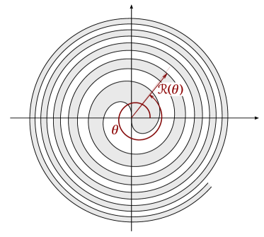
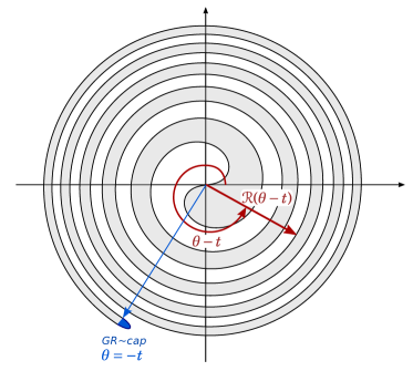
Figure 1. Left: The Yin Yang soliton in polar coordinates. Right: The Truncated Yin Yang soliton at time $t\ll 0$. The bulk of the curve consists of an initial segment of the Yin–Yang curve rotated counterclockwise by an angle $t$, which has two ends. These ends are connected by a small cap in the shape of a translating soliton (the so-called “Grim Reaper”) located at polar angle $\theta=-t$.

In section 2 of this paper we construct an approximate solution to CSF, by truncating the Yin–Yang solution at polar angle $\alpha(t)$, and connecting the two ends with a small cap whose shape is approximately that of a rotated and rescaled copy of the Grim Reaper soliton. See Figure 1 (right).

To determine how to choose the angle $\alpha(t)$ we estimate the speed $V$ of the cap at time $t$. Since the cap is approximately a Grim Reaper, its speed is related to its width $w$ by $V=\pi/w$. The width $w$ is approximated by

$$w\approx{\mathcal{R}}(\alpha(t)-t+\tfrac{\pi}{2})-{\mathcal{R}}(\alpha(t)-t-\tfrac{\pi}{2})\approx{\mathcal{R}}^{\prime}(\alpha(t)-t)\,\pi,$$

so that the cap moves with speed

$$V\approx\frac{\pi}{w}\approx\frac{1}{{\mathcal{R}}^{\prime}(\alpha(t)-t).}$$

On the other hand, far away from the center, the arms of the Yin-Yang spiral are close to circular. The cap, which moves with angular velocity $-\alpha^{\prime}(t)$ along a near circle with radius ${\mathcal{R}}(\alpha(t)-t)$, therefore has velocity $V\approx-\alpha^{\prime}(t){\mathcal{R}}(\alpha(t)-t)$. It follows that $\alpha^{\prime}(t)\approx-1/({\mathcal{R}}{\mathcal{R}}^{\prime})$. Since the asymptotics (1.1) imply ${\mathcal{R}}{\mathcal{R}}^{\prime}\approx 1$, we end up with

(1.2) $$\alpha^{\prime}(t)=-1+o(1),\qquad\alpha(t)=-t+o(t).$$

For any $t<0$ we let $\Omega(t)\subset\mathbb{R}^{2}$ be the region given in Polar Coordinates by

(1.3) $$\Omega(t)=\Bigl{\{}(r\cos\theta,r\sin\theta)\;\big{|}\;t\leqslant\theta\leqslant-t,\;{\mathcal{R}}(\theta-t-\tfrac{\pi}{2})\leqslant r\leqslant{\mathcal{R}}(\theta-t+\tfrac{\pi}{2})\Bigr{\}}$$

We will call the boundary curve $\partial\Omega(t)$ the truncated Yin-Yang curve. It consists of a segment of the rotating Yin-Yang curve and a straight line segment that connects the two ends at $\theta=-t$.

Main Theorem. There exists a compact ancient solution $\{C(t)\mid t<0\}$ to Curve Shortening which for $t\to-\infty$ is uniformly close to the truncated Yin-Yang curve in the sense that if $\Lambda(t)$ is the bounded region enclosed by $C(t)$ then

$$\mathrm{Area}(\Lambda(t)\triangle\Omega(t))\lesssim|t|^{-1+\delta}\qquad(t\to-\infty)$$

for every $\delta>0$.

The construction follows a pattern similar to the construction of ancient solutions in [3, 10], namely, construct a sequence of “really old solutions” $\{{\mathcal{C}}_{n}(t)\mid-n\leqslant t\leqslant t_{0}\}$ of Curve Shortening and extract a convergent subsequence whose limit is the desired ancient solution. In section 2 we first construct an ancient approximate solution $\{{\mathcal{C}}_{*}(t)\mid-\infty<t<0\}$ of Curve Shortening, i.e. a family of curves for which

(1.4) $${\mathcal{E}}{\stackrel{{\scriptstyle\textrm{def}}}{{=}}}\int_{-\infty}^{t_{0}}\int_{{\mathcal{C}}_{*}(t)}\left|V-\kappa\right|\,ds\,dt<\infty.$$

Then we consider a sequence of solutions $\{{\mathcal{C}}_{n}(t)\mid-n\leqslant t<t_{0}\}$ of Curve Shortening whose initial curves ${\mathcal{C}}_{n}(-n)$ are chosen increasingly close to the approximate solution ${\mathcal{C}}_{*}(-n)$ at time $-n$, in the sense that the area between ${\mathcal{C}}_{*}(-n)$ and ${\mathcal{C}}_{n}(-n)$ tends to zero as $n\to\infty$. Arguing as in [3, 10] we observe that the area between the solutions ${\mathcal{C}}_{n}(t)$ and the approximate solution ${\mathcal{C}}_{*}(t)$ is bounded in terms of the “error” ${\mathcal{E}}$ and the area between the initial curves ${\mathcal{C}}_{*}(-n)$ and ${\mathcal{C}}_{n}(-n)$. Since the curves we deal with in this paper are not graphical the area estimate is a bit more complicated than in [3, 10]. In section 3 we present a more general estimate that generalizes the Altschuler-Grayson [2] area bounds for Space Curve Shortening. Finally, in section 4 we show how this bound allows us to extract a convergent subsequence of the very old solutions ${\mathcal{C}}_{n}(t)$, and provides enough control to conclude that the resulting limit satisfies the description in the Main Theorem.

In appendix A we recall the derivation of the Yin-Yang soliton, and obtain its asymptotic expansion at infinity.

Comparison with the construction in [4]. The idea to construct ancient solutions as a limit of a sequence of very old solutions is natural. In [4] the same strategy is also followed, but the core of the proof where one controls the sequence of old solutions is quite different. While the approach in our paper follows the method of area comparison established in [3], the arguments in [4] proceed by carefully controlling a sequence of old solutions via an exponential barrier for the bulk of the solution. Thereafter stability of the tip is established in [4] using a blow-up argument, combined with the uniqueness of the Grim Reaper as possible limit.

2. Construction of the cap

2.1. Parametrized curves and the Curve Shortening deficit

An evolving family of curves is a map $X:(t_{0},t_{1})\times\mathbb{R}\to\mathbb{R}^{2}$ for which $X_{p}(t,p)\neq 0$ for all $(t,p)$. For such a family we define

$$ds=\|X_{p}(t,p)\|\,dp,\qquad\frac{d}{ds}=\frac{1}{\|X_{p}(t,p)\|}\frac{d}{dp}\;.$$

The normal velocity and curvature of the family $X$ are

$$V=\left\langle X_{t},JX_{s}\right\rangle,\qquad\kappa=\left\langle X_{ss},JX_{s}\right\rangle=\left\langle\frac{X_{pp}}{\|X_{p}\|^{2}},\frac{JX_{p}}{\|X_{p}\|}\right\rangle$$

where $J=\left(\begin{smallmatrix}0&-1\\ 1&0\end{smallmatrix}\right)$ represents counterclockwise rotation by $\frac{\pi}{2}$. By definition, the parameterized family of curves $X$ satisfies Curve Shortening if $V=\kappa$. If it does not, then we measure the “discrepancy with curve shortening” in terms of the form

(2.1) $$|V-\kappa|\,ds=\left|\Bigl{\langle}X_{t}-\frac{X_{pp}}{\|X_{p}\|^{2}},JX_{p}\Bigr{\rangle}\right|\,dp$$

The error ${\mathcal{E}}$ is obtained by integrating this form over the curve and in time.

We write ${{\boldsymbol{e}}_{1}}=(1,0)$, ${{\boldsymbol{e}}_{2}}=(0,1)$ for the standard basis for $\mathbb{R}^{2}$. In this basis counterclockwise rotation by $\theta$ is given by

$$e^{\theta J}=\begin{pmatrix}\cos\theta&-\sin\theta\\ \sin\theta&\cos\theta\end{pmatrix}.$$

We will use the rotated frame $\{{{\boldsymbol{E}}_{1}}(\theta),{{\boldsymbol{E}}_{2}}(\theta)\}=\{e^{\theta J}{{\boldsymbol{e}}_{1}},e^{\theta J}{{\boldsymbol{e}}_{2}}\}$, which satisfy

$${{\boldsymbol{E}}_{1}}^{\prime}(\theta)={{\boldsymbol{E}}_{2}}(\theta),\qquad{{\boldsymbol{E}}_{2}}^{\prime}(\theta)=-{{\boldsymbol{E}}_{1}}(\theta).$$

2.2. $Z$ or $(u,v)$-coordinates

We expect the tip of the ancient solution to be located near the point $R(t){{\boldsymbol{E}}_{1}}(-t)$, and to have width $\sim R^{-1}$, where

$$R=R(t){\stackrel{{\scriptstyle\textrm{def}}}{{=}}}{\mathcal{R}}(-2t).$$

Thus we introduce new, time dependent, coordinates $Z=u{{\boldsymbol{e}}_{1}}+v{{\boldsymbol{e}}_{2}}$ related to the cartesian coordinates $X=(x_{1},x_{2})$ via

(2.2) $$X=e^{-tJ}\{R{{\boldsymbol{e}}_{1}}+R^{-1}Z\},\text{ i.e. }Z=R\bigl{\{}e^{tJ}X-R{{\boldsymbol{e}}_{1}}\bigr{\}}.$$

2.3. The inner and outer Yin-Yang arms

The region on one side of the Yin-Yang curve is foliated by rotated copies of the curve. At time $t\in\mathbb{R}$ the leaves of this foliation are parametrized by

(2.3) $$Y(\theta,t,y)={\mathcal{R}}(\theta-t+y){{\boldsymbol{E}}_{1}}(\theta)$$

where $y\in[-\pi/2,\pi/2]$ determines the leaf, and $\theta\in(t-y,\infty)$ is the polar angle on the leaf. The inner and outer arms of the region that contains our ancient solution correspond to $y=\pm\pi/2$. See Figure 2.

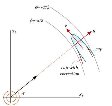
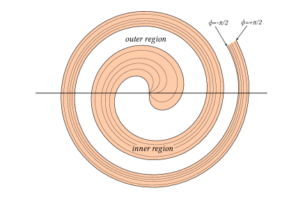
Figure 2. Left: The $(u,v)$ coordinates.  Right: The Yin Yang foliation at time $t=0$.

2.4. Lemma

For any $M>0$ there is a $t_{M}<0$ such that if $t\leqslant t_{M}$, then the segments of the Yin-Yang leaves $Y(\theta,t,y)$ with $|\theta+t|\leqslant M\tau^{-1}\ln\tau$ are graphs in $(u,v)$ coordinates of the form $u=U_{y}(t,v)$, at least if $t\leqslant t_{M}$. Moreover, the functions $U_{y}(t,v)$ satisfy

(2.4) $$U_{y}(t,v)=y-\frac{y^{2}+v^{2}-2v}{2\tau}+{\mathcal{O}}(\tau^{-2+\delta})$$

for all $\delta>0$, where $\tau=-4t$.

Proof.

We begin with the defining equations

(2.5) $${\mathcal{R}}(\theta-t+y){{\boldsymbol{E}}_{1}}(\theta)=e^{-tJ}\bigl{\{}R{{\boldsymbol{e}}_{1}}+R^{-1}Z\bigr{\}}=e^{-tJ}\bigl{\{}(R+u/R){{\boldsymbol{e}}_{1}}+v/R\,{{\boldsymbol{e}}_{2}}\bigr{\}}.$$

Multiply with $e^{tJ}$ on both sides:

$${\mathcal{R}}(\theta-t+y){{\boldsymbol{E}}_{1}}(\theta+t)=R{{\boldsymbol{e}}_{1}}+R^{-1}Z=(R+u/R){{\boldsymbol{e}}_{1}}+v/R\,{{\boldsymbol{e}}_{2}}.$$

Here the left hand side is the polar form of the right hand side. Under our assumptions $R^{2}\sim\tau$ and $|u|\ll\tau$, so $1+u/R^{2}>0$, and hence we have

(2.6) $${\mathcal{R}}(\theta-t+y)^{2}=R^{2}+2u+\frac{u^{2}+v^{2}}{R^{2}},\qquad\theta+t=\arctan\frac{v/R^{2}}{1+u/R^{2}}.$$

Since $\alpha\mapsto{\mathcal{R}}(\alpha)^{2}$ is a monotone function, the first equation in (2.6) can be solved for $y$. Using the asymptotic expansion in appendix A.3 we get

(2.7) $$2(\theta-t+y)={\mathcal{R}}^{2}+2{\mathcal{R}}^{-2}+{\mathcal{O}}({\mathcal{R}}^{-4}),$$

where ${\mathcal{R}}={\mathcal{R}}(\theta-t+y)$. Replace ${\mathcal{R}}^{2}$ by the expression in (2.6), to get

$$2(\theta-t+y)=R^{2}+2u+\frac{u^{2}+v^{2}+2}{R^{2}}+{\mathcal{O}}\bigl{(}v^{2}R^{-4}\bigr{)}.$$

To eliminate $\theta$ we expand the second equation in (2.6),

$$\theta+t=\frac{v}{R^{2}}+{\mathcal{O}}\bigl{(}v^{2}R^{-4}\bigr{)}.$$

Hence

(2.8) $$2y =2(\theta-t+y)-2(\theta+t)+4t (-4t=\tau)$$

$$=R^{2}-\tau+2u+\frac{u^{2}+v^{2}-2v+2}{R^{2}}+{\mathcal{O}}\bigl{(}v^{2}R^{-4}\bigr{)}.$$

Expand $R=R(t)={\mathcal{R}}(-2t)$ in powers of $\tau=-4t$ using (A.7):

$$R^{2}={\mathcal{R}}(-2t)^{2}=\tau\left(1-2\tau^{-2}+{\mathcal{O}}(\tau^{-3})\right)$$

and substitute this in (2.8) to get

$$2y=2u+\frac{u^{2}+v^{2}-2v}{\tau}+{\mathcal{O}}(v^{2}R^{-4}).$$

By assumption we have $|v|\lesssim\ln\tau$ and $R\sim\sqrt{\tau}$, so $v^{2}R^{-4}={\mathcal{O}}(\tau^{-2+\delta})$ for any $\delta>0$.

If $\tau$ is sufficiently large then the above equation has a unique solution $u=U_{y}(t,v)$ with

$$u=y-\frac{u^{2}+v^{2}-2v}{2\tau}+{\mathcal{O}}(\tau^{-2+\delta})=y-\frac{y^{2}+v^{2}-2v}{2\tau}+{\mathcal{O}}(\tau^{-2+\delta}).\qed$$

2.5. General ansatz for the cap

We now construct the cap by assuming that it is given by

(2.9) $$X(t,p)=e^{-tJ}\bigl{\{}R{{\boldsymbol{e}}_{1}}+\varepsilon Z(t,p)\bigr{\}},\text{ with }R(t){\stackrel{{\scriptstyle\textrm{def}}}{{=}}}{\mathcal{R}}(-2t),\;\varepsilon(t)=\frac{1}{R(t)},$$

and by computing its deviation from Curve Shortening (2.1)

$$(V-\kappa)ds=\langle X_{t}-X_{ss},JX_{s}\rangle ds=\Bigl{\langle}X_{t}-\frac{X_{pp}}{\|X_{p}\|^{2}},JX_{p}\Bigr{\rangle}\;dp{\stackrel{{\scriptstyle\textrm{def}}}{{=}}}W\,dp$$

In the following computations it will be convenient to abbreviate

$$R_{\theta}(t)={\mathcal{R}}^{\prime}(-2t),$$

so that $R^{\prime}(t)=-2R_{\theta}(t)$.

The space derivatives of $X$ are

$$X_{p}=e^{-tJ}\varepsilon Z_{p}\qquad X_{pp}=e^{-tJ}\varepsilon Z_{pp}.$$

The time derivative has a few more terms:

$$X_{t}=e^{-tJ}\left\{-2R_{\theta}{{\boldsymbol{e}}_{1}}-R{{\boldsymbol{e}}_{2}}+\varepsilon^{\prime}Z-\varepsilon JZ+\varepsilon Z_{t}\right\}$$

Express $W=\langle X_{t}-X_{pp}/\|X_{p}\|^{2},JX_{p}\rangle$ in terms of $Z$, keeping in mind that $\varepsilon=R^{-1}$,

(2.10) $$W=\left\langle\varepsilon^{2}Z_{t}-\frac{Z_{pp}}{\|Z_{p}\|^{2}},JZ_{p}\right\rangle-\langle{{\boldsymbol{e}}_{1}},Z_{p}\rangle\\ +2\varepsilon R_{\theta}\langle{{\boldsymbol{e}}_{2}},Z_{p}\rangle+\varepsilon\varepsilon^{\prime}\langle Z,JZ_{p}\rangle-\varepsilon^{2}\langle Z,Z_{p}\rangle.$$

We look for a cap in the form of a normal perturbation of the Grim Reaper curve, i.e. we assume

(2.11) $$Z(t,p)=G(p)+f(t,p)JG_{p}(p)$$

where

$$G(p)=-\arcsin(\tanh p){{\boldsymbol{e}}_{1}}-\ln(\cosh p){{\boldsymbol{e}}_{2}}$$

is the arclength parametrization of the Grim Reaper.

Since $G$ is an arclength parametrization $G_{p},JG_{p}$ are unit tangent and normal to the Grim Reaper. Specifically,

$$G_{p}=-\frac{1}{\cosh p}{{\boldsymbol{e}}_{1}}-\tanh p{{\boldsymbol{e}}_{2}}.$$

The parametrization $G(p)$ traces the Grim Reaper out from right to left. Furthermore, the curvature vector of the Grim Reaper is

$$G_{pp}(p)=\kappa(p)JG_{p},\text{ where }\kappa(p)=\frac{1}{\cosh p}.$$

2.6. Detailed computation of $W$ on the cap

We have

$$Z_{t} =f_{t}JG_{p}$$

$$Z_{p} =G_{p}+f_{p}JG_{p}+fJG_{pp}=(1-\kappa f)G_{p}+f_{p}JG_{p}$$

$$JZ_{p} =-f_{p}G_{p}+(1-\kappa f)JG_{p}$$

$$\|Z_{p}\|^{2} =(1-\kappa f)^{2}+f_{p}^{2}=1-2\kappa f+\kappa^{2}f^{2}+f_{p}^{2}$$

$$Z_{pp} =-(\kappa_{p}f+2\kappa f_{p})G_{p}+\bigl{(}f_{pp}+\kappa-\kappa^{2}f\bigr{)}JG_{p}$$

Substituting in (2.10), and using $\kappa=1/\cosh p$, we get

$$\left\langle\varepsilon^{2}Z_{t},JZ_{p}\right\rangle =\varepsilon^{2}(1-\kappa f)f_{t}$$

$$\Bigl{\langle}\frac{Z_{pp}}{\|Z_{p}\|^{2}},JZ_{p}\Bigr{\rangle} =\frac{(1-\kappa f)(f_{pp}+\kappa(1-\kappa f))+\kappa_{p}ff_{p}+2\kappa f_{p}^{2}}{1-2\kappa f+\kappa^{2}f^{2}+f_{p}^{2}}$$

$$\langle{{\boldsymbol{e}}_{1}},Z_{p}\rangle =-\kappa(1-\kappa f)+f_{p}\tanh p.$$

Thus after substituting and expanding we find

(2.12) $$W=\varepsilon^{2}(1-\kappa f)f_{t}-\frac{\kappa+f_{pp}-2\kappa^{2}f-\kappa ff_{pp}+\kappa_{p}ff_{p}+\kappa^{3}f^{2}+2\kappa f_{p}^{2}}{1-2\kappa f+\kappa^{2}f^{2}+f_{p}^{2}}+\kappa(1-\kappa f)$$

$$-f_{p}\tanh p-\varepsilon^{2}\langle Z,Z_{p}\rangle+2\varepsilon R_{\theta}\langle{{\boldsymbol{e}}_{2}},Z_{p}\rangle+\varepsilon\varepsilon^{\prime}\langle Z,JZ_{p}\rangle.$$

We will choose $f(t,p)$ so as to make $W$ integrable in space and time. To find $f$ we linearize the expression for $W$ and solve the resulting first order equation for $f$. It turns out that one solution is of the form $f(t,p)=\tau^{-1}F(p)$ for a function $F$ that is of polynomial growth for $|p|\to\infty$. We restrict our attention to the region

(2.13) $$|p|\leqslant 2K\ln\tau,\qquad\tau\gg 1,$$

where $K=100$ is a fixed, largish, constant. We will assume that $f$ and its derivatives are bounded by

(2.14) $$|f|+|f_{p}|+|f_{pp}|+\tau|f_{t}|\lesssim\tau^{-1+\delta}\text{ for }|p|\leqslant 2K\ln\tau.$$

Here, and in what follows, when we write estimates for remainder terms of the form ${\mathcal{O}}(\tau^{-m+\delta})$, the estimate is implicitly meant to hold “for all $\delta>0$.”

The bound (2.14) will certainly hold if $f(t,p)=\tau^{-1}F(p)$ for some function $F(p)$ for which $F(p)$, $F^{\prime}(p)$, and $F^{\prime\prime}(p)$ grow polynomially as $p\to\pm\infty$.

We now consider the many terms in (2.12) that add up to $W$. To begin, we have for $|p|\leqslant 2K\ln\tau$,

$$\varepsilon^{2}(1-\kappa f)f_{t}={\mathcal{O}}(\tau^{-2+\delta}),$$

and also

$$\frac{-\kappa ff_{pp}+\kappa_{p}ff_{p}+\kappa^{3}f^{2}+2\kappa f_{p}^{2}}{1-2\kappa f+\kappa^{2}f^{2}+f_{p}^{2}}={\mathcal{O}}(\tau^{-2+\delta})\text{ for any }\delta>0.$$

It follows from $Z=G+fJG_{p}$ that

$$Z=G+{\mathcal{O}}\bigl{(}\tau^{-1+\delta}\bigr{)},\qquad Z_{p}=G_{p}+{\mathcal{O}}\bigl{(}\tau^{-1+\delta}\bigr{)}.$$

Hence, for $|p|\leqslant 2K\ln\tau$,

$$\|G(p)\| \lesssim\ln\tau \varepsilon^{2}\langle Z,Z_{p}\rangle =\tau^{-1}\langle G,G_{p}\rangle+{\mathcal{O}}\bigl{(}\tau^{-2+\delta}\bigr{)}$$

$$\varepsilon R_{\theta}\langle{{\boldsymbol{e}}_{2}},Z_{p}\rangle =\tau^{-1}\langle{{\boldsymbol{e}}_{2}},G_{p}\rangle+{\mathcal{O}}\bigl{(}\tau^{-2+\delta}\bigr{)} \quad\varepsilon\varepsilon^{\prime}\langle Z,JZ_{p}\rangle ={\mathcal{O}}\bigl{(}\tau^{-2+\delta}\bigr{)}.$$

In this computation we have used the expansions $\varepsilon=R(t)^{-1}={\mathcal{R}}(-2t)^{-1}=\tau^{-1/2}+{\mathcal{O}}(\tau^{-3/2})$ and $R_{\theta}={\mathcal{R}}^{\prime}(-2t)=\tau^{-1/2}+{\mathcal{O}}(\tau^{-3/2})$ that follow from the expansions of ${\mathcal{R}}(\theta)$ and ${\mathcal{R}}^{\prime}(\theta)$ in appendix A.

So far we have

$$W={\mathcal{O}}\bigl{(}\tau^{-2+\delta}\bigr{)}-\frac{\kappa+f_{pp}-2\kappa^{2}f}{1-2\kappa f+\kappa^{2}f^{2}+f_{p}^{2}}+\kappa(1-\kappa f)-f_{p}\tanh p$$

$$+\tau^{-1}\langle 2{{\boldsymbol{e}}_{2}}-G,G_{p}\rangle$$

We can simplify the fraction (for $|p|\leqslant 2K\ln\tau$) by using

$$\frac{1}{1-2\kappa f+\kappa^{2}f^{2}+f_{p}^{2}}=1+2\kappa f-\kappa^{2}f^{2}-f_{p}^{2}+\frac{(-2\kappa f+\kappa^{2}f^{2}+f_{p}^{2})^{2}}{1-2\kappa f+\kappa^{2}f^{2}+f_{p}^{2}}=1+2\kappa f+{\mathcal{O}}\bigl{(}\tau^{-2+\delta}\bigr{)}$$

which implies

$$\frac{\kappa+f_{pp}-2\kappa^{2}f}{1-2\kappa f+\kappa^{2}f^{2}+f_{p}^{2}}=\kappa+2\kappa^{2}f+f_{pp}-2\kappa^{2}f+{\mathcal{O}}\bigl{(}\tau^{-2+\delta}\bigr{)}=\kappa+f_{pp}+{\mathcal{O}}\bigl{(}\tau^{-2+\delta}\bigr{)},$$

and hence

$$W=-f_{pp}-\tanh(p)f_{p}-\kappa^{2}f+\frac{1}{\tau}\langle 2{{\boldsymbol{e}}_{2}}-G,G_{p}\rangle+{\mathcal{O}}(\tau^{-2+\delta}).$$

2.7. Computation of the correction term

We look to perturb the Grim Reaper with a term of the form

$$f(t,p)=\frac{F(p)}{\tau},$$

where $F$ is a solution of

$${\mathcal{L}}F{\stackrel{{\scriptstyle\textrm{def}}}{{=}}}F_{pp}+\tanh(p)F_{p}+\kappa^{2}F=\langle 2{{\boldsymbol{e}}_{2}}-G,G_{p}\rangle.$$

The linear operator can be factored

$${\mathcal{L}}=\frac{d^{2}}{dp^{2}}+\tanh(p)\frac{d}{dp}+\frac{1}{\cosh^{2}(p)}=\frac{d}{dp}\circ\frac{1}{\cosh p}\circ\frac{d}{dp}\circ\cosh(p)$$

while we also have

$$\langle 2{{\boldsymbol{e}}_{2}}-G,G_{p}\rangle=\frac{d}{dp}\bigl{\langle}2{{\boldsymbol{e}}_{2}}-\tfrac{1}{2}G,G\bigr{\rangle},$$

all of which allows us to solve the equation for $F$:

(2.15) $$F(p)=\frac{A}{\cosh p}+B\tanh p+\int_{0}^{p}\frac{\cosh r}{\cosh p}\bigl{\langle}2{{\boldsymbol{e}}_{2}}-\tfrac{1}{2}G(r),G(r)\bigr{\rangle}\,dr.$$

It appears that the first term is of no use, so we set $A=0$. The resulting function $F(p)$ is an odd function of $p$. We use the asymptotic behavior of $\langle 2{{\boldsymbol{e}}_{2}}-\tfrac{1}{2}G,G\rangle$ for large $p$ to find an expansion for the integral as $p\to+\infty$.

Consider

$$I{\stackrel{{\scriptstyle\textrm{def}}}{{=}}}\int_{0}^{p}\frac{\cosh r}{\cosh p}\bigl{\langle}2{{\boldsymbol{e}}_{2}}-\tfrac{1}{2}G(r),G(r)\bigr{\rangle}\,dr.$$

The explicit expression for $G$ implies

$$\langle{{\boldsymbol{e}}_{2}},G(r)\rangle =-\ln\cosh r$$

$$\|G(r)\|^{2} =\bigl{(}\ln\cosh r\bigr{)}^{2}+\bigl{(}\arcsin\tanh r\bigr{)}^{2}=\bigl{(}\ln\cosh r\bigr{)}^{2}+\frac{\pi^{2}}{4}+{\mathcal{O}}(e^{-r})\qquad(r\to\infty).$$

To compute $I$ we substitute $\lambda=\ln\cosh p$, $\mu=\ln\cosh r$, which leads to

$$I=-\int_{0}^{\lambda}e^{\mu-\lambda}\bigl{\{}2\mu+\tfrac{1}{2}\mu^{2}+\tfrac{\pi^{2}}{8}+{\mathcal{O}}(e^{-\mu})\bigr{\}}\frac{d\mu}{\sqrt{1-e^{-2\mu}}}$$

The integrand is singular but integrable at $\mu=0$. To deal with this singularity split

$$(1-e^{-2\mu})^{-1/2}=1+\bigl{[}(1-e^{-2\mu})^{-1/2}-1\bigr{]},\text{ with }0\leqslant(1-e^{-2\mu})^{-1/2}-1\lesssim\frac{1}{\sqrt{\mu}}e^{-2\mu}.$$

Replacing $(1-e^{-2\mu})^{-1/2}$ by $1$ therefore introduces an extra term that is bounded by ${\mathcal{O}}(e^{-\lambda})$. Hence we have

$$I ={\mathcal{O}}(e^{-\lambda})-\int_{0}^{\lambda}e^{\mu-\lambda}\bigl{\{}2\mu+\tfrac{1}{2}\mu^{2}+\tfrac{\pi^{2}}{8}+{\mathcal{O}}(e^{-\mu})\bigr{\}}\,d\mu$$

$$={\mathcal{O}}(\lambda^{3}e^{-\lambda})-\int_{0}^{\lambda}e^{\mu-\lambda}\bigl{\{}2\mu+\tfrac{1}{2}\mu^{2}+\tfrac{\pi^{2}}{8}\bigr{\}}\,d\mu$$

$$={\mathcal{O}}(\lambda^{3}e^{-\lambda})-\bigl{\{}2\lambda+\tfrac{1}{2}\lambda^{2}+\tfrac{\pi^{2}}{8}\bigr{\}}+\bigl{\{}2+\lambda\bigr{\}}-\{1\}$$

$$=-\tfrac{1}{2}\lambda^{2}-\lambda-\tfrac{\pi^{2}}{8}+1+{\mathcal{O}}(\lambda^{3}e^{-\lambda})$$

Thus, for large $p$ we get

$$F(p)=B-\tfrac{1}{2}(\ln\cosh p)^{2}-\ln\cosh p-\tfrac{\pi^{2}}{8}+1+{\mathcal{O}}\bigl{(}|p|^{3}e^{-|p|}\bigr{)}\qquad(p\to+\infty).$$

Since $F(p)$ is an odd function we also have

$$F(p)=-\left\{B-\tfrac{1}{2}(\ln\cosh p)^{2}-\ln\cosh p-\tfrac{\pi^{2}}{8}+1\right\}+{\mathcal{O}}\bigl{(}|p|^{3}e^{-|p|}\bigr{)}\qquad(p\to-\infty).$$

Applying this to $Z=G+\tau^{-1}F(p)JG_{p}$ we get for the two components $u$ and $v$ of $Z$ as $p\to\pm\infty$:

$$u(t,p) =-\arcsin\tanh p+\frac{1}{\tau}F(p)\tanh p=\mp\frac{\pi}{2}+\frac{1}{\tau}F(p)\tanh p+{\mathcal{O}}(e^{-|p|})$$

$$v(t,p) =-\ln\cosh p-\frac{1}{\tau}\frac{F(p)}{\cosh p}=-\ln\cosh p+{\mathcal{O}}(|p|^{3}e^{-|p|})$$

We can again eliminate $p$ when $p$ is large by using

$$\ln\cosh p=-v+{\mathcal{O}}(p^{2}e^{-|p|}),\qquad(p\to\pm\infty)$$

which leads to

(2.16) $$u(t,p)=\mp\frac{\pi}{2}-\frac{v^{2}-2v+\pi^{2}/4+2(1+B)}{2\tau}+{\mathcal{O}}(|p|^{3}e^{-|p|})\qquad(p\to\pm\infty)$$

We now determine $B$ by matching (2.16) with the representation of the Yin-Yang arms in $(u,v)$ coordinates that we found in (2.4). Setting $y=\mp\pi/2$ in (2.4) we find for the outer and inner Yin-Yang arms

(2.17) $$u=\mp\frac{\pi}{2}-\frac{\pi^{2}/4+v^{2}-2v}{2\tau}+{\mathcal{O}}(\tau^{-2+\delta})$$

If $|p|\geqslant\frac{K}{2}\ln\tau$ then $|p|^{3}e^{-|p|}={\mathcal{O}}(\tau^{-K/2+\delta})=o(\tau^{-2+\delta})$, and therefore the two expansions (2.16),(2.17) match if

(2.18) $$B=-1.$$

To summarize, we choose the cap to be given by

(2.19) $$X(t,p)=e^{-tJ}\bigl{\{}R(t){{\boldsymbol{e}}_{1}}+\frac{1}{R(t)}Z(t,p)\bigr{\}}$$

with

(2.20) $$Z(t,p)=G(p)+\frac{F(p)}{\tau}JG_{p}(p)$$

and, from (2.15),

(2.21) $$F(p)=\,-\tanh p+\int_{0}^{p}\frac{\cosh r}{\cosh p}\bigl{\langle}2{{\boldsymbol{e}}_{2}}-\tfrac{1}{2}G(r),G(r)\bigr{\rangle}\,dr$$

2.8. Definition of the smooth interpolation of cap and arms

In the $(u,v)$ coordinates, according to (2.4), the Yin-Yang arms are given by

$$u=U_{\pm}(t,v)\text{ for }|v|\leqslant 3K\ln\tau$$

where we abbreviate $U_{\pm}(t,v)=U_{\pm\pi/2}(t,v)$. In the same $(u,v)$ coordinates the ends of the cap are given by (2.16) with, $B=-1$, i.e.

$$u=h_{\pm}(t,v)\text{ for }\tfrac{1}{2}K\ln\tau\leqslant-v\leqslant 2K\ln\tau.$$

We constructed the cap so that both $U_{\pm}$ and $h_{\pm}$ have the same asymptotic behavior, namely,

(2.22) $$U_{\pm}(t,v),h_{\pm}(t,v)=\pm\frac{\pi}{2}-\frac{1}{\tau}\Bigl{\{}\tfrac{1}{2}v^{2}-v+\pi^{2}/8\Bigr{\}}+{\mathcal{O}}(\tau^{-2+\delta}).$$

Choose a smooth nondecreasing function $\eta:\mathbb{R}\to\mathbb{R}$ with $\eta(u)=0$ for $u\leqslant\frac{1}{2}$ and $\eta(u)=1$ for $u\geqslant 2$, and define

$$k_{\pm}(t,v) =\eta\Bigl{(}\frac{-v}{\ln\tau}\Bigr{)}U_{\pm}(t,v)+\left\{1-\eta\Bigl{(}\frac{-v}{\ln\tau}\Bigr{)}\right\}h_{\pm}(t,v)$$

(2.23) $$=U_{\pm}(t,v)+\eta\Bigl{(}\frac{-v}{\ln\tau}\Bigr{)}\bigl{(}U_{\pm}(t,v)-h_{\pm}(t,v)\bigr{)}.$$

The graphs of these two functions are $Z$-coordinate representations of curve segments that smoothly interpolate between the two ends of the cap and the two Yin-Yang arms. The two segments are parametrized by

$$X_{\pm}(t,v)=e^{-tJ}\bigl{\{}R{{\boldsymbol{e}}_{1}}+R^{-1}Z_{\pm}(t,v)\bigr{\}}\text{ with }Z_{\pm}(t,v)=k_{\pm}(t,v){{\boldsymbol{e}}_{1}}+v{{\boldsymbol{e}}_{2}}.$$

It follows from (2.10) that the Curve Shortening Deficit for such curves is given by $(\kappa-V)ds=W_{v}dv$ with

(2.24) $$W_{v}[k]=-R^{-2}k_{t}+\frac{k_{vv}}{1+k_{v}^{2}}-k_{v}+2\frac{R_{\theta}}{R}+2\frac{R_{\theta}}{R^{3}}(vk_{v}-k)-R^{-2}(v+kk_{v}).$$

2.9. Derivative bounds for $U_{\pm}$, $h_{\pm}$, $k_{\pm}$

Careful scrutiny of the construction of $U_{\pm}(t,v)$ and $h_{\pm}(t,v)$ shows that the remainder terms ${\mathcal{O}}(\tau^{-2+\delta})$ in (2.22) may be differentiated. This implies that the functions $U_{\pm}$ and $h_{\pm}$ satisfy

(2.25) $$|k_{vv}|+|k_{v}|+|k_{t}|\lesssim\frac{\ln\tau}{\tau}\lesssim\tau^{-1+\delta}$$

for $\frac{1}{2}\ln\tau\leqslant-v\leqslant 2K\ln\tau$, and large enough $\tau$.

The derivatives of the gluing function $\eta(v/\ln\tau)$ are

$$\eta_{v}=-\frac{\eta^{\prime}(-v/\ln\tau)}{\ln\tau},\quad\eta_{vv}=\frac{\eta^{\prime\prime}(-v/\ln\tau)}{(\ln\tau)^{2}},\quad\eta_{t}=-\frac{4v\eta^{\prime}(-v/\ln\tau)}{(\ln\tau)^{2}},$$

so they are bounded by

$$|\eta_{v}|+|\eta_{vv}|+|\eta_{t}|\lesssim\bigl{(}\ln\tau\bigr{)}^{-1}$$

for $\frac{1}{2}\ln\tau\leqslant-v\leqslant 2K\ln\tau$, and large enough $\tau$.

It follows that the interpolating functions $k_{\pm}=\eta U_{\pm}+(1-\eta)h_{\pm}$ also satisfy (2.25).

2.10. Estimating $W_{v}[k_{\pm}]$

We show that

(2.26) $$\big{|}W_{v}[k_{\pm}]\big{|}\lesssim\tau^{-2+\delta}$$

holds in the region $\frac{1}{2}K\ln\tau\leqslant-v\leqslant 2K\ln\tau$, for sufficiently large $\tau$.

If $k$ is any of the functions $U_{\pm},h_{\pm},k_{\pm}$ then we have

$$\frac{|k_{v}^{2}k_{vv}|}{1+k_{v}^{2}}\leqslant|k_{v}^{2}k_{vv}|\lesssim\tau^{-3+\delta},\quad R^{-2}|kk_{v}|\lesssim\tau^{-3+\delta},\text{ and }-R^{-2}|k_{t}|\lesssim\tau^{-2+\delta}.$$

Furthermore $|k|\lesssim 1$, $|vk_{v}|\lesssim\tau^{-1+\delta}$, and $R_{\theta}\sim R^{-1}\lesssim\tau^{-1/2}$ lead to

$$\frac{R_{\theta}}{R^{3}}|vk_{v}-k|\lesssim\tau^{-2}.$$

Hence

$$W_{v}[k]=k_{vv}-k_{v}+2\frac{R_{\theta}}{R}-vR^{-2}+{\mathcal{O}}(\tau^{-2+\delta})$$

holds for all six functions $k\in\{U_{\pm},h_{\pm},k_{\pm}\}$.

To simplify our notation we drop the $\pm$ subscript for now and expand the derivatives of $k=\eta U+(1-\eta)h$ (with $U=U_{\pm}$ and $h=h_{\pm}$),

$$k_{v}=\eta U_{v}+(1-\eta)h_{v}+\eta_{v}(U-h),$$

$$k_{vv}=\eta U_{vv}+(1-\eta)h_{vv}+2\eta_{v}(U-h)_{v}+\eta_{vv}(U-h).$$

Since we have matched the two cap ends with the Yin-Yang arms, it follows from (2.22) that the difference $U-h$ and its derivatives are bounded by

$$|U-h|+|(U-h)_{v}|+|(U-h)_{vv}|\lesssim\tau^{-2+\delta}.$$

Together these inequalities give us the desired estimate for $W_{v}[k_{\pm}]$, namely

$$W_{v}[k] =W_{v}[\eta U+(1-\eta)h]$$

$$=\bigl{(}\eta U+(1-\eta)h\bigr{)}_{vv}-\bigl{(}\eta U+(1-\eta)h\bigr{)}_{v}+2\frac{R_{\theta}}{R}-vR^{-2}+{\mathcal{O}}(\tau^{-2+\delta})$$

$$=\eta W_{v}[U]+(1-\eta)W_{v}[h]+{\mathcal{O}}(\tau^{-2+\delta})$$

(2.27) $$={\mathcal{O}}(\tau^{-2+\delta}).$$

Definition 2.1 (The Approximate Solution).

Let ${\mathcal{C}}_{*}(t):(-\infty,-T)\times\mathbb{R}\rightarrow\mathbb{R}^{2}$ for some sufficiently large $T>0$ be the family of smooth curves formed by the concatenation of the Yin-Yang leaves $Y(\theta,t,-\tfrac{\pi}{2})$, $Y(\theta,t,+\tfrac{\pi}{2})$ cut off in a neighborhood of $R(t){{\boldsymbol{E}}_{1}}(-t)$ and glued to the cap $X(t,p)$ defined by the ansatzes (2.9) and (2.11), with $f(t,p)=\tau^{-1}F(p)$ and $F(p)$ given by (2.15) with $A=0$ and $B=-1$. The gluing between the arms of the cap and the two Yin-Yang segments is given by the interpolation $k_{\pm}(t,v)$ in (2.8), which is done in a neighborhood of $R(t){{\boldsymbol{E}}_{1}}(-t)$.

Lemma 2.1.

The error

$${\mathcal{E}}(T)=\int_{-\infty}^{-T}\int_{{\mathcal{C}}_{*}(t)}\left|V-\kappa\right|\,ds\,dt<\infty$$

is finite on the approximate solution ${\mathcal{C}}_{*}(t):(-\infty,-T)\times\mathbb{R}\rightarrow\mathbb{R}^{2}$ given by Definition 2.1.

Proof.

It suffices to show that the Curve Shortening Deficit $|V-\kappa|ds$ is $L^{1}$-integrable in space and time on three regions: the cap, the transition region discussed in §2.8, and the unmodified Yin-Yang curve. Since the Yin-Yang curve is a solution to Curve Shortening Flow, the deficit $|V-\kappa|ds=0$, which leaves only cap and the transition region as contributing to the error.

The cap, given by the expressions (2.19), (2.20), and (2.21), is defined on the region $|p|\leq 2K\ln\tau$, where $p$ is the arc-length coordinate $p$ for the grim reaper $G(p)$. In §2.6-§2.7, the Curve Shortening Deficit $|V-\kappa|ds$ is written in terms of $p$ as $Wdp$, and it is shown to be $W={\mathcal{O}}(\tau^{-2+\delta})$ for $\delta>0$. Integrating over the cap, we have

$$\int_{\text{cap}}|V-\kappa|ds\leq\int_{-2K\ln\tau}^{2K\ln\tau}Wdp\leq 4K\ln\tau{\mathcal{O}}(\tau^{-2+\delta})={\mathcal{O}}(\tau^{-2+\delta}).$$

This quantity is integrable in time, and thus the contribution to the error ${\mathcal{E}}$ on the cap is bounded.

In §2.8, the Curve Shortening Deficit on the transition region is written in terms of the parameter $v$ as $W_{v}[k]dv$ on the interval $\tfrac{1}{2}\leq-v\leq 2K\ln\tau$. Furthermore, in (2.10) it is shown that $W_{v}[k]={\mathcal{O}}(\tau^{-2+\delta})$. Integrating over both curves in the transition region, we have

$$\int_{\text{trns. reg.}}|V-\kappa|ds=2\int_{\tfrac{1}{2}K\ln\tau}^{2K\ln\tau}W_{v}[k]dv\leq 3K\ln\tau{\mathcal{O}}(\tau^{-2+\delta})={\mathcal{O}}(\tau^{-2+\delta}).$$

As before, this is integrable in time and thus the contribution to the error is bounded. Therefore, the sum of the integrals of the deficit over each region is ${\mathcal{O}}(\tau^{-2+\delta})$. This completes the proof of the lemma. ∎

3. Area decreasing property of Space Curve Shortening

In 1991 Altschuler and Grayson [2] observed that for two solutions of space curve shortening the area of the minimal surface spanning them is non increasing. Here we elaborate on this and prove a similar result without using the existence of the minimal surface.

3.1. Moving space curves

For an immersed curve $X:\mathbb{R}\to\mathbb{R}^{n}$ one defines the arc length one-form $ds$ and the arc length derivative $\partial_{s}$ of any quantity $f:\mathbb{R}\to\mathbb{R}$ by

$$ds=\|X_{p}\|\,dp,\text{ and }\frac{\partial f}{\partial s}=\frac{1}{\|X_{p}\|}\frac{\partial f}{\partial p}.$$

The unit tangent and curvature of the curve are $X_{s}=\frac{X_{p}}{\|X_{p}\|}$ and $X_{ss}$.

A moving family of space curves is a map $X:(t_{0},t_{1})\times\mathbb{R}\to\mathbb{R}^{n}$. The family evolves by Curve Shortening if it satisfies $X_{t}^{\perp}=X_{ss}$, i.e., if for some smooth function $\lambda(t,p)$ one has

(3.1) $$X_{t}=X_{ss}+\lambda X_{s}=\frac{1}{\|X_{p}\|}\frac{\partial}{\partial p}\Bigl{(}\frac{X_{p}}{\|X_{p}\|}\Bigr{)}+\lambda\frac{X_{p}}{\|X_{p}\|}$$

Since $X_{s}\perp X_{ss}$, one can always find $\lambda$ from $\lambda=\langle X_{t},X_{s}\rangle$.

3.2. Evolution of arc length and the commutator $[\partial_{t},\partial_{s}]$

The following are commonly used relations. We record them here for completeness, and also because we allow the velocity $X_{t}$ of the parametrizations to have a nonvanishing tangential component. Assuming that $X_{t}=X_{ss}+\lambda X_{s}$ one has

(3.2) $$\partial_{t}\|X_{p}\|=(\lambda_{s}-\kappa^{2})\|X_{p}\|,\qquad\frac{\partial}{\partial t}ds=(\lambda_{s}-\kappa^{2})ds=d\lambda-\kappa^{2}ds,$$

and

(3.3) $$[\partial_{t},\partial_{s}]=(-\lambda_{s}+\kappa^{2})\partial_{s}.$$

Proof.

We have

$$\frac{\partial}{\partial t}\|X_{p}\|=\Bigl{\langle}\frac{X_{p}}{\|X_{p}\|},X_{tp}\Bigr{\rangle}=\langle X_{s},X_{tp}\rangle=\langle X_{s},X_{ts}\rangle\|X_{p}\|,$$

and hence

$$\frac{\partial}{\partial t}ds=\frac{\partial}{\partial t}\bigl{(}\|X_{p}\|dp\bigr{)}=\langle X_{s},X_{tp}\rangle dp=\bigl{\langle}X_{s},X_{ts}\bigr{\rangle}ds.$$

The evolution equation $X_{t}=X_{ss}+\lambda X_{s}$ then implies

$$\bigl{\langle}X_{s},X_{ts}\bigr{\rangle}=\langle X_{s},X_{t}\rangle_{s}-\bigl{\langle}X_{ss},X_{t}\bigr{\rangle}=\lambda_{s}-\bigl{\langle}X_{ss},X_{ss}+\lambda X_{s}\bigr{\rangle}=\lambda_{s}-\|X_{ss}\|^{2}=\lambda_{s}-\kappa^{2},$$

which directly implies (3.2). Using (3.2) we get

$$[\partial_{t},\partial_{s}]=\left[\partial_{t},\|X_{p}\|^{-1}\partial_{p}\right]=-\frac{\partial_{t}\|X_{p}\|}{\|X_{p}\|^{2}}\partial_{p}=-(\lambda_{s}-\kappa^{2})\partial_{s}.\qed$$

3.3. Dependence on a parameter

Let $[\epsilon_{0},\epsilon_{1}]\subset\mathbb{R}$ be some parameter interval, and let $X:[\epsilon_{0},\epsilon_{1}]\times(t_{0},t_{1})\times\mathbb{R}\to\mathbb{R}^{n}$ be a family of moving curves that depends on a parameter $\epsilon\in[\epsilon_{0},\epsilon_{1}]$. We compute the evolution of the first variation

$$X_{\epsilon}=\partial_{\epsilon}X(\epsilon,t,p).$$

Throughout the computation we will assume that the parametrization $X$ is such that

(3.4) $$X_{\epsilon}\perp X_{p}(\epsilon,t,p)\text{ for all $(\epsilon,t,p)$}$$

For any given parametrization $\widetilde{X}$ one can find a reparametrization $\varphi(\epsilon,t,p)$ so that $X(\epsilon,t,p)=\widetilde{X}(\epsilon,t,\varphi(\epsilon,t,p))$ satisfies (3.4).

If $X:[\epsilon_{0},\epsilon_{1}]\times[0,1]\to\mathbb{R}^{n}$ is injective with $X_{\varepsilon}\perp X_{p}$, then the double integral

$$\int_{\epsilon_{0}}^{\epsilon_{1}}\int_{p=0}^{1}\|X_{\epsilon}\|\,ds\,d\epsilon\qquad(\text{where }ds=\|X_{p}\|dp)$$

is the area (2-dim Hausdorff measure) of the image $X([\epsilon_{0},\epsilon_{1}]\times[0,1])$. If $X$ merely satisfies $X_{\epsilon}\perp X_{p}$, without necessarily being injective, then the area formula implies that the double integral is bounded from below, by

(3.5) $$\ell(X){\stackrel{{\scriptstyle\textrm{def}}}{{=}}}\int_{\epsilon_{0}}^{\epsilon_{1}}\int_{p=0}^{1}\|X_{\epsilon}\|\,ds\,d\epsilon\geqslant\mathcal{H}^{2}(X([\epsilon_{0},\epsilon_{1}]\times[0,1]))$$

We will call the integral $\ell(X)$ the length of the homotopy $X$, and we will show that Curve Shortening decreases the length of homotopies.

The following improvement of the inequality $\|X_{\epsilon}\|_{s}\leqslant\|X_{\epsilon s}\|$ (which follows from the Cauchy-Schwarz inequality) will be useful.

3.4. Lemma

Assuming (3.4) we have

$$\bigl{(}\|X_{\epsilon}\|_{s}\bigr{)}^{2}\leqslant\|X_{\epsilon s}\|^{2}-\langle X_{ss},X_{\epsilon}\rangle^{2}.$$

Proof.

Split $X_{\epsilon s}$ into tangential and orthogonal components:

$$X_{\epsilon s}=P+\langle X_{\epsilon s},X_{s}\rangle X_{s}$$

Since $X_{\epsilon}\perp X_{s}$ we have $\langle X_{\epsilon s},X_{s}\rangle=\partial_{s}\langle X_{\epsilon},X_{s}\rangle-\langle X_{\epsilon},X_{ss}\rangle=-\langle X_{\epsilon},X_{ss}\rangle$. Therefore

$$X_{\epsilon s}=P-\langle X_{\epsilon},X_{ss}\rangle X_{s},$$

and thus

$$\|X_{\epsilon s}\|^{2}=\|P\|^{2}+\langle X_{\epsilon},X_{ss}\rangle^{2}.$$

On the other hand

$$\|X_{\epsilon}\|_{s}=\Bigl{\langle}\frac{X_{\epsilon}}{\|X_{\epsilon}\|},X_{\epsilon s}\Bigr{\rangle}=\Bigl{\langle}\frac{X_{\epsilon}}{\|X_{\epsilon}\|},P\Bigr{\rangle}\leqslant\|P\|,$$

where we have again used that $X_{s}\perp X_{\epsilon}$. Combining these observations we arrive at

$$\bigl{(}\|X_{\epsilon}\|_{s}\bigr{)}^{2}-\|X_{\epsilon s}\|^{2}\leqslant\|P\|^{2}-\|X_{\epsilon s}\|^{2}=-\langle X_{\epsilon},X_{ss}\rangle^{2},$$

as claimed. ∎

3.5. The commutator $[\partial_{\epsilon},\partial_{s}]$

Assuming (3.4) one has

$$[\partial_{\epsilon},\partial_{s}]=\langle X_{ss},X_{\epsilon}\rangle\partial_{s}\text{ and }[\partial_{\epsilon},\partial_{s}^{2}]=2\langle X_{ss},X_{\epsilon}\rangle\partial_{s}^{2}+\langle X_{ss},X_{\epsilon}\rangle_{s}\partial_{s}$$

Proof.

The computation follows the same pattern as the derivation of (3.3). Here we have no equation for $X_{\epsilon}$, but we do know that $X_{\epsilon}\perp X_{s}$. Thus

$$\partial_{\epsilon}\|X_{p}\|=\left\langle\frac{X_{p}}{\|X_{p}\|},X_{p\epsilon}\right\rangle=\langle X_{s},X_{\epsilon p}\rangle=\langle X_{s},X_{\epsilon s}\rangle\|X_{p}\|=-\langle X_{ss},X_{\epsilon}\rangle\|X_{p}\|.$$

Apply this to $\partial_{s}=\|X_{p}\|^{-1}\partial_{p}$ to get the commutator $[\partial_{\epsilon},\partial_{s}]$. The other commutator follows from expanding $[\partial_{\epsilon},\partial_{s}^{2}]=[\partial_{\epsilon},\partial_{s}]\partial_{s}+\partial_{s}[\partial_{\epsilon},\partial_{s}]$. ∎

3.6. Lemma

The length of the first variation $X_{\epsilon}$ satisfies the differential inequality

$$\partial_{t}\|X_{\epsilon}\|-\lambda\partial_{s}\|X_{\epsilon}\|\leqslant\partial_{s}^{2}\|X_{\epsilon}\|+\kappa^{2}\|X_{\epsilon}\|.$$

Proof.

Differentiating the evolution equation (3.1) for $X$ we get

$$\partial_{t}X_{\epsilon}=\partial_{\epsilon}X_{t} =\partial_{\epsilon}\left(X_{ss}+\lambda X_{s}\right)$$

$$=X_{\epsilon ss}+2\langle X_{ss},X_{\epsilon}\rangle X_{ss}+\langle X_{ss},X_{\epsilon}\rangle_{s}X_{s}+\lambda_{\epsilon}X_{s}+\lambda\partial_{\epsilon}X_{s}.$$

Hence

$$\partial_{t}X_{\epsilon}-\lambda\partial_{s}X_{\epsilon} =X_{\epsilon ss}+2\langle X_{ss},X_{\epsilon}\rangle X_{ss}+\langle X_{ss},X_{\epsilon}\rangle_{s}X_{s}+\lambda_{\epsilon}X_{s}+\lambda[\partial_{\epsilon},\partial_{s}]X$$

$$=X_{\epsilon ss}+2\langle X_{ss},X_{\epsilon}\rangle X_{ss}+\left\{\langle X_{ss},X_{\epsilon}\rangle_{s}+\lambda_{\epsilon}+\lambda\langle X_{ss},X_{\epsilon}\rangle\right\}X_{s}$$

We next compute the evolution of $\|X_{\epsilon}\|^{2}$, keeping in mind that $X_{\epsilon}\perp X_{s}$:

$$(\partial_{t}-\lambda\partial_{s})\|X_{\epsilon}\|^{2} =2\langle X_{\epsilon},\partial_{t}X_{\epsilon}-\lambda\partial_{s}X_{\epsilon}\rangle$$

$$=2\langle X_{\epsilon},X_{\epsilon ss}\rangle+4\langle X_{ss},X_{\epsilon}\rangle^{2}$$

$$=\bigl{(}\|X_{\epsilon}\|^{2}\bigr{)}_{ss}-2\|X_{\epsilon s}\|^{2}+4\langle X_{ss},X_{\epsilon}\rangle^{2}$$

$$=2\|X_{\epsilon}\|\,\|X_{\epsilon}\|_{ss}+2\bigl{(}\|X_{\epsilon}\|_{s}\bigr{)}^{2}-2\|X_{\epsilon s}\|^{2}+4\langle X_{ss},X_{\epsilon}\rangle^{2}.$$

At this point we use Lemma 3.4, to get

$$(\partial_{t}-\lambda\partial_{s})\|X_{\epsilon}\|^{2}\leqslant 2\|X_{\epsilon}\|\,\|X_{\epsilon}\|_{ss}+2\langle X_{ss},X_{\epsilon}\rangle^{2}.$$

Since $(\partial_{t}-\lambda\partial_{s})\|X_{\epsilon}\|^{2}=2\|X_{\epsilon}\|(\partial_{t}-\lambda\partial_{s})\|X_{\epsilon}\|$, we have

$$\partial_{t}\|X_{\epsilon}\|-\lambda\partial_{s}\|X_{\epsilon}\|\leqslant\|X_{\epsilon}\|_{ss}+\Bigl{\langle}X_{ss},\frac{X_{\epsilon}}{\|X_{\epsilon}\|}\Bigr{\rangle}^{2}\|X_{\epsilon}\|\leqslant\|X_{\epsilon}\|_{ss}+\kappa^{2}\|X_{\epsilon}\|.\qed$$

3.7. Contractive property of Curve Shortening

If $X^{0},X^{1}:[t_{0},t_{1}]\times[0,1]\to\mathbb{R}^{n}$ are two solutions of Curve Shortening (3.1), then a homotopy $\{X^{\epsilon}:0\leqslant\epsilon\leqslant 1\}$ of solutions to Curve Shortening connecting them is, by definition, a map $X:[0,1]\times[t_{0},t_{1}]\times[0,1]\to\mathbb{R}^{n}$ such that $(t,p)\mapsto X(\varepsilon,t,p)$ is a solution of Curve Shortening with $X^{\epsilon}(t,p)=X(\epsilon,t,p)$ for $\epsilon\in\{0,1\}$.

Given any homotopy $X^{\epsilon}$ between solutions $X^{0},X^{1}$ of Curve Shortening, one can always find a reparametrization $\widetilde{X}^{\epsilon}(t,p)=X^{\epsilon}(t,\varphi(\epsilon,t,p))$ for which $\partial_{\epsilon}\widetilde{X}^{\epsilon}\perp\partial_{s}\widetilde{X}^{\epsilon}$ holds pointwise. We will call such a homotopy a normal homotopy.

Our main observation in this section is the following: if $X^{\epsilon}$ is a normal homotopy between solutions $X^{0},X^{1}$ of Curve Shortening, then one has for each $\epsilon\in[0,1]$ and $t\in(t_{0},t_{1})$

(3.6) $$\frac{d}{dt}\int_{p=0}^{1}\|\partial_{\epsilon}X(\epsilon,t,p)\|\,ds\leqslant 0$$

and

(3.7) $$\int_{\epsilon=0}^{1}\int_{p=0}^{1}\|\partial_{\epsilon}X(\epsilon,t_{1},p)\|\,ds\,d\epsilon\leqslant\int_{\epsilon=0}^{1}\int_{p=0}^{1}\|\partial_{\epsilon}X(\epsilon,t_{0},p)\|\,ds\,d\epsilon$$

Proof.

We use (3.2) and Lemma 3.6 to differentiate under the integral:

$$\frac{d}{dt}\int_{p=0}^{1}\|X_{\epsilon}\|\,ds\leqslant\int\left\{\|X_{\epsilon}\|_{ss}+\kappa^{2}\|X_{\epsilon}\|+\lambda\|X_{\epsilon}\|_{s}+(\lambda_{s}-\kappa^{2})\|X_{\epsilon}\|\right\}\,ds\\ =\int\bigl{\{}\|X_{\epsilon}\|_{s}+\lambda\|X_{\epsilon}\|\bigr{\}}_{s}\,ds=0.$$

This implies (3.6). Integration in $\epsilon$ and in time then leads to (3.7). ∎

3.8. Deviation from an approximate solution

We now consider the case of two moving curves $X^{0},X^{1}:[t_{0},t_{1}]\times[0,1]\to\mathbb{R}^{n}$ with the same initial value, i.e. with $X^{0}(t_{0},p)=X^{1}(t_{0},p)$ for all $p\in[0,1]$. We assume that $X^{1}$ is a solution of Curve Shortening but allow $X^{0}$ to be a general moving curve. We measure its deviation from Curve Shortening in terms of

(3.8) $$\Delta{\stackrel{{\scriptstyle\textrm{def}}}{{=}}}\int_{t_{0}}^{t_{1}}\int_{p=0}^{1}\bigl{\|}(\partial_{t}X^{0})^{\perp}-\partial_{s}^{2}X^{0}\bigr{\|}\,ds\,dt.$$

In the case of plane curves $X:[t_{0},t_{1}]\times[0,1]\to\mathbb{R}^{2}$, we have $\partial_{t}(X^{0})^{\perp}=VJX^{0}_{s}$, where $V$ is the normal velocity of the curve $X^{0}$. Therefore the integrand in (3.8) is

$$\bigl{\|}(\partial_{t}X^{0})^{\perp}-\partial_{s}^{2}X^{0}\bigr{\|}\,ds=|V-\kappa|\,ds.$$

The quantity $\Delta$ therefore coincides with the “error” ${\mathcal{E}}$ defined in (1.4).

Assume that for each $\epsilon\in[t_{0},t_{1}]$ there is a smooth solution $(t,p)\mapsto X(\epsilon,t,p)$ of Curve Shortening that is defined for $t\in[\epsilon,t_{1}]$, and that has initial value $X(\epsilon,\epsilon,p)=X^{0}(\epsilon,p)$. After reparametrizing we may assume that $X_{\epsilon}\perp X_{p}$ holds point-wise. Then the final values of these solutions, i.e. the curves $p\mapsto X(\epsilon,t_{1},p)$ form a normal homotopy from $X^{0}(t_{1},\cdot)$ to $X^{1}(t_{1},\cdot)$. We will now show that

(3.9) $$\int_{\epsilon=t_{0}}^{t_{1}}\int_{p=0}^{1}\|\partial_{\epsilon}X(\epsilon,t_{1},p)\|\,ds\,d\epsilon\leqslant\Delta.$$

Proof.

Our argument is a nonlinear version of the Variation of Constants Formula, or of Duhamel’s principle.

For $\epsilon\in[t_{0},t_{1}]$ we consider

$$E(\epsilon){\stackrel{{\scriptstyle\textrm{def}}}{{=}}}\int_{\bar{\epsilon}=t_{0}}^{\epsilon}\int_{0}^{1}\|\partial_{\epsilon}X(\bar{\epsilon},t_{1},p)\|\,ds\,d\bar{\epsilon}.$$

Then

$$E^{\prime}(\epsilon)=\int_{0}^{1}\|\partial_{\epsilon}X(\epsilon,t_{1},p)\|\,ds$$

The contraction property (3.6) implies

$$\int_{0}^{1}\|\partial_{\epsilon}X(\epsilon,t_{1},p)\|\,ds\leqslant\int_{0}^{1}\|\partial_{\epsilon}X(\epsilon,\epsilon,p)\|\,ds.$$

We compute $X_{\epsilon}(\epsilon,\epsilon,p)$ by differentiating the relation $X(\epsilon,\epsilon,p)=X^{0}(\epsilon,p)$ with respect to $\epsilon$:

$$\bigl{(}\partial_{t}X^{0}\bigr{)}(\epsilon,p)=\frac{\partial X^{0}(\epsilon,p)}{\partial\epsilon}=\frac{\partial X(\epsilon,\epsilon,p)}{\partial\epsilon}=X_{\epsilon}(\epsilon,\epsilon,p)+X_{t}(\epsilon,\epsilon,p).$$

Since $(t,p)\mapsto X(\epsilon,t,p)$ evolves by Curve Shortening, we have $X_{t}(\epsilon,\epsilon,p)=X_{ss}(\epsilon,\epsilon,p)+\lambda X_{s}$. By definition of $X$ we have $X(\epsilon,\epsilon,p)=X^{0}(\epsilon,p)$, so $X_{ss}(\epsilon,\epsilon,p)=X^{0}_{ss}(\epsilon,p)$.

We have parameterized the homotopy $X(\epsilon,t,p)$ so that $X_{\epsilon}\perp X_{p}$, and therefore

$$\partial_{\epsilon}X(\epsilon,\epsilon,p)=\bigl{(}\partial_{t}X^{0}(\epsilon,p)\bigr{)}^{\perp}-X^{0}_{ss}(\epsilon,p).$$

Hence

$$E^{\prime}(\epsilon)\leqslant\int_{0}^{1}\|\partial_{\epsilon}X(\epsilon,\epsilon,p)\|\,ds=\int_{0}^{1}\left\|\bigl{(}\partial_{t}X^{0}(\epsilon,p)\bigr{)}^{\perp}-X^{0}_{ss}(\epsilon,p)\right\|\,ds$$

Integrate over $\epsilon\in[t_{0},t_{1}]$ to recover (3.9). ∎

3.9. Application to plane Curve Shortening

Let $X^{0},X^{1}:[t_{0},t_{1}]\times[0,1]\to\mathbb{R}^{2}$ be two moving curves that are embedded at all time. Assume $X^{1}$ evolves by Curve Shortening, and assume that initially $X^{1}$ lies in the closed region enclosed by $X^{0}$, i.e. for all $p\in[0,1]$ the point $X^{1}(t_{0},p)$ lies in the region enclosed by the simple curve $p\mapsto X^{0}(t_{0},p)$.

Assume furthermore that at each time $t_{*}\in[t_{0},t_{1}]$ the area enclosed by $p\mapsto X^{0}(t_{*},p)$ is at least $2\pi(t_{1}-t_{*})$. By the Gage-Hamilton-Grayson theorem this guarantees that the solution to Curve Shortening starting at $X^{0}(t_{*},\cdot)$ exists until time $t_{1}$.

We now consider two homotopies $A$ and $B$ of evolving curves. The first is the homotopy defined in the proof in the previous section 3.8, i.e. for each $\epsilon\in[t_{0},t_{1}]$ we consider the solution $(t,p)\mapsto X(\epsilon,t,p)$ to Curve Shortening defined for $t\in[\epsilon,t_{1}]$ and starting from $X(\epsilon,\epsilon,p)=X^{0}(\epsilon,p)$. Our first homotopy is then the family of final curves $A(\epsilon,p)=X(\epsilon,t_{1},p)$ of these solutions. In section 3.8 we showed that the length of the homotopy $A$ is bounded from above by

$$\ell(A)=\int_{t_{0}}^{t_{1}}\int_{0}^{1}\|A_{\epsilon}(\epsilon,p)\|\,ds\,d\epsilon\leqslant\int_{t_{0}}^{t_{1}}\int_{0}^{1}\left\|(\partial_{t}X^{0})^{\perp}-X^{0}_{ss}\right\|\,ds\,dt.$$

The second homotopy is constructed by evolving a homotopy between the two initial curves $p\mapsto X^{j}(t_{0},p)$ ($j=0,1$). Since $X^{1}$ initially lies inside $X^{0}$ we can choose the homotopy $(\epsilon,p)\mapsto\bar{X}(\epsilon,t_{0},p)$ so that its length is exactly the area of the region between the two initial curves, and so that the curve $p\mapsto\bar{X}(\epsilon,t_{0},p)$ lies inside the curve $p\mapsto\bar{X}(\epsilon^{\prime},t_{0},p)$ if $0\leqslant\epsilon\leqslant\epsilon^{\prime}\leqslant 1$. Given this initial homotopy let $(t,p)\mapsto\bar{X}(\epsilon,t,p)$ be the solution to Curve Shortening starting at $\bar{X}(\epsilon,t_{0},p)$. Since all initial curves enclose $X^{1}(t_{0},p)$ the corresponding solutions exist for $t\in[t_{0},t_{1}]$, and possibly longer. Our second homotopy is now $B(\epsilon,p)=\bar{X}(\epsilon,t_{1},p)$. As explained in section 3.7, the length of the homotopy $B$ is bounded by the length of the initial homotopy $(\epsilon,p)\mapsto\bar{X}(\epsilon,t_{0},p)$. We had chosen this initial homotopy so that its length is exactly the area between the two curves $p\mapsto X^{0}(t_{0},p)$ and $p\mapsto X^{1}(t_{0},p)$.

By concatenating the two homotopies $A$ and $B$ we obtain a combined homotopy $A\#B$ between $p\mapsto X^{0}(t_{1},p)$ and $p\mapsto X^{1}(t_{1},p)$. The length of this homotopy is bounded by

$$\ell(A\#B)=\ell(A)+\ell(B)\leqslant\text{Area between $X^{0}(t_{0},\cdot)$ and $X^{1}(t_{0},\cdot)$}\\ +\int_{t_{0}}^{t_{1}}\int_{0}^{1}\left\|(\partial_{t}X^{0})^{\perp}-X^{0}_{ss}\right\|\,ds\,dt$$

If $\Omega^{0}(t)$ and $\Omega^{1}(t)$ are the regions enclosed by $X^{0}(t,\cdot)$ and $X^{1}(t,\cdot)$, then the homotopy $A\#B$ between the two curves at time $t_{1}$ must pass through each point in the interior of the symmetric difference $\Omega^{0}(t_{1})\triangle\Omega^{1}(t_{1})$, as one sees by considering the winding numbers of the curves in the homotopy around any point in $\Omega^{0}(t_{1})\triangle\Omega^{1}(t_{1})$. It follows that the area of $\Omega^{0}(t_{1})\triangle\Omega^{1}(t_{1})$ is a lower bound for the length of the homotopy $A\#B$, and thus we conclude that

(3.10) $$\text{Area of }\Omega^{0}(t_{1})\triangle\Omega^{1}(t_{1})\leqslant\\ \text{Area between $X^{0}(t_{0},\cdot)$ and $X^{1}(t_{0},\cdot)$}+\int_{t_{0}}^{t_{1}}\int_{0}^{1}\left\|(\partial_{t}X^{0})^{\perp}-X^{0}_{ss}\right\|\,ds\,dt.$$

4. Convergence

In this section, we obtain uniform curvature bounds on a sequence of “really old solutions” $\{{\mathcal{C}}_{j}(t)\}$ and extract a subsequence of solutions that converges locally smoothly to an ancient solution of curve shortening flow (CSF).

Theorem 4.1.

There exists a $T$ such that for any $T^{*}>T$, the curvatures $|\kappa_{j}|$ of the “really old solutions” $\{{\mathcal{C}}_{j}(t)\}_{j}$ are bounded independently of $j$ on the interval $[-T^{*}-1/4,-T^{*}]$.

The strategy to obtain these bounds is as follows: a) decompose an element ${\mathcal{C}}_{j}(t)$ of this sequence into the union of several graph representations, b) use the $L^{1}$ bound on the error to obtain $L^{\infty}$ estimates for these graphs, and c) apply the standard estimates for divergence-form quasilinear parabolic equations to establish a uniform curvature bound.

Let $T^{*}>0$ be a large positive number, which may be increased as necessary throughout this section. The obvious candidates for the sequence of “really old solutions” are the CSF solutions defined on $[-j,-T^{*}]$ starting at ${\mathcal{C}}_{*}(-j)$ at time $-j$ — call these $\Gamma_{j}(t)$. At any time $t\in[-j,-T^{*}]$, the unsigned area enclosed by the curves ${\mathcal{C}}_{*}(t)$ and $\Gamma_{j}(t)$ is bounded by the quantity

$$\int_{-j}^{t}\int_{{\mathcal{C}}_{*}(\tau)}|V-\kappa|ds\;d\tau.$$

By Lemma 2.1, this quantity is in $L^{1}$ and given $\epsilon>0$, we can find $T^{*}>0$ such that

$${\mathcal{E}}(T^{*})=\int_{-\infty}^{-T^{*}}\int_{{\mathcal{C}}_{*}(\tau)}|V-\kappa|ds\;d\tau<\epsilon.$$

By (3.10), this estimate gives a uniform bound on the unsigned area between $\Gamma_{j}(t)$ and ${\mathcal{C}}_{*}(t)$ for any sufficiently large $j$ and $t<-T^{*}$, whenever defined.

For simplicity of calculation, we consider an alternative sequence of “really old solutions” $\{{\mathcal{C}}_{j}(t)\}$, called “square-profile approximations”, which do not satisfy the initial condition ${\mathcal{C}}_{j}(-j)={\mathcal{C}}_{*}(-j)$. They are constructed as follows: Let $[\vartheta_{*}^{-}(t),\vartheta_{*}^{+}(t)]$ be the interval of polar angles that contain the approximate solution at a given time $t$. Let $r={\mathcal{R}}(\theta)$ be the central branch of the Yin-Yang foliation, so the Yin-Yang solution is given by the two branches $r={\mathcal{R}}(\theta+\pi/2-t)$ and $r={\mathcal{R}}(\theta-\pi/2-t)$. We define ${\mathcal{C}}_{j}(t)$ to be the solution of curve shortening which at time $t=-j$ is given by

• Two arms of the Yin-Yang soliton $r={\mathcal{R}}(\theta-\pi/2-t)={\mathcal{R}}(\theta-\pi/2+j)$, and $r={\mathcal{R}}(\theta+\pi/2-t)={\mathcal{R}}(\theta+\pi/2+j)$ truncated at $\theta=\vartheta_{*}^{+}(-j)$;

• a straight line segment connecting the two arms of the Yin-Yang soliton. This segment is part of the ray $\theta=\vartheta_{*}^{+}(-j)$.

Notice that at each time $t$ along the flow, the square-profile approximations ${\mathcal{C}}_{j}(t)$ enclose the curves $\Gamma_{j}(t)$, the CSF solutions starting from ${\mathcal{C}}_{*}(-j)$, and that the area bounded by these two solutions stays constant along the flow, for all $t\in[-j,-T^{*}]$. The area $A_{j}$ between ${\mathcal{C}}_{j}(-j)$ and ${\mathcal{C}}_{*}(-j)$ is small and goes to zero as $j\to\infty$. Thus, the area between the old solution ${\mathcal{C}}_{j}(t)$ with the “square initial data” and the approximate solution ${\mathcal{C}}_{*}(t)$ is bounded by

$$\mathop{\textrm{Area}}({\mathcal{C}}_{j}(t),{\mathcal{C}}_{*}(t))\leqslant A_{j}+\int_{-j}^{t}\int_{{\mathcal{C}}_{*}(\tau)}|V-\kappa|\,ds\,d\tau.$$

In order to improve these area bounds to $L^{\infty}$ bounds, we will use the geometry of the ${\mathcal{C}}_{j}(t)$ and several properties of CSF. In particular, we often appeal to the maximum principle and the following Sturmian property for intersections of curve shortening flows.

Theorem 4.2.

Consider two CSF solutions $\gamma_{0},\gamma_{1}:[T_{1},T_{2})\times[0,1]\rightarrow\mathbb{R}^{2}$, for which

$$\partial\gamma_{0}(t)\cap\gamma_{1}(t)=\partial\gamma_{1}(t)\cap\gamma_{0}(t)=\varnothing$$

holds for any $t\in[T_{1},T_{2})$. Then the number of intersections of $\gamma_{0}(t)$ and $\gamma_{1}(t)$ is a finite and non-increasing function of $t\in(T_{1},T_{2})$. It decreases whenever $\gamma_{0}$ and $\gamma_{1}$ have a tangency.

There is a useful related theorem for inflections points.

Theorem 4.3.

Let $\gamma:[T_{1},T_{2})\times S^{1}\rightarrow\mathbb{R}^{2}$ be a solution of CSF. Then, for any $t\in(T_{1},T_{2})$, $\gamma(t)$ has at most a finite number of inflection points, and this number does not increase with time. In fact, it drops whenever the curvature $\kappa$ has a multiple zero.

While the curves ${\mathcal{C}}_{j}(t)$ are not convex, we do have a one sided curvature bound.

Theorem 4.4.

If $\kappa$ is the curvature of a counterclockwise oriented parametrization $X$ of the curves ${\mathcal{C}}_{j}(t)$, then

$$\kappa-\langle X,X_{s}\rangle>0.$$

Proof.

Assuming that the parametrization $X$ is normal ($X_{t}\perp X_{s}$), the curvature evolves by

$$\kappa_{t}=\kappa_{ss}+\kappa^{3}.$$

A short computation using $X_{t}=X_{ss}$ and $\|X_{s}\|=1$ shows that

$$\bigl{(}\partial_{t}-\partial_{s}^{2}\bigr{)}\|X\|^{2}=2\langle X_{t},X\rangle-2\langle X_{ss},X\rangle-2\|X_{s}\|^{2}=-2.$$

Differentiating with respect to arclength, using the commutator $[\partial_{t},\partial_{s}]=\kappa^{2}\partial_{s}$, and also $\partial_{s}\|X\|^{2}=2\langle X,X_{s}\rangle$ we get

$$\partial_{t}\langle X,X_{s}\rangle=\partial_{s}^{2}\langle X,X_{s}\rangle+\kappa^{2}\langle X,X_{s}\rangle.$$

Hence $\kappa$ and $\langle X,X_{s}\rangle$ satisfy the same linear equation. Therefore $\sigma=\kappa-\langle X,X_{s}\rangle$ also satisfies

$$\sigma_{t}=\sigma_{ss}+\kappa^{2}\sigma.$$

The quantity $\sigma$ vanishes on the rotating soliton (see the appendix).

The square-profile initial curves ${\mathcal{C}}_{j}(-j)$ consist of two arcs. One is the Yin-Yang soliton, so on this arc we have $\sigma=0$. The other arc is the radial line segment on the ray $\theta=\vartheta_{*}^{+}(-j)$. On this segment we clearly have $\kappa=0$. Since we orient ${\mathcal{C}}_{j}$ counterclockwise, $X$ and $X_{s}$ are parallel with opposite directions; i.e. $-\langle X,X_{s}\rangle>0$. Hence $\sigma>0$ on the line segment. Finally, the initial curve ${\mathcal{C}}_{j}(-j)$ is not smooth, having two corners where the line segment and Yin-Yang arms meet. If one rounds these corners off by replacing them with small circle arcs with radius $\rho\ll 1$, then the curvature of these arcs will be $\kappa=\rho^{-1}\gg 1$, so that $\sigma>0$ on the circular arcs, provided $\rho$ is sufficiently small. The resulting curve has $\sigma=0$ on the Yin-Yang arms, and $\sigma>0$ on the line segment, as well as the small circular arcs. The solution to CS starting from the modified initial curve therefore has $\sigma>0$. Letting $\rho\searrow 0$ we conclude that $\sigma>0$ also holds on ${\mathcal{C}}_{j}(t)$. ∎

With Theorem 4.2, we can decompose the solutions ${\mathcal{C}}_{j}(t)$ into exactly two graphs over the polar angle parameter.

Lemma 4.5.

For any $t\in(-j,-T^{*}]$, there is an interval $[\vartheta^{-}_{j}(t),\vartheta^{+}_{j}(t)]$ such that the curve ${\mathcal{C}}_{j}(t)$ can be written as the union of two graphs of polar functions, $R_{j}^{-}(\theta,t)$ and $R_{j}^{+}(\theta,t)$ defined for $\theta\in[\vartheta^{-}_{j}(t),\vartheta^{+}_{j}(t)]$. The functions $t\mapsto\vartheta^{-}_{j}(t)$ and $t\mapsto\vartheta^{+}_{j}(t)$ are strictly increasing and decreasing, respectively.

Proof.

By the maximum principle, the “really old solutions” ${\mathcal{C}}_{j}(t)$ will be contained inside of the Yin-Yang curve. The Sturmian property, Theorem 4.2, tells us that the number of intersections of ${\mathcal{C}}_{j}(t)$ and the rays $\theta=\theta_{0}\in\mathbb{R}$ is non-increasing, and only decreases when there is a tangency. This implies that the desired graph decomposition exists. These two graphs are bounded above and below by the branches of the Yin-Yang soliton on their polar interval of definition, $[\vartheta^{-}_{j}(t),\vartheta^{+}_{j}(t)]$. ∎

Similarly, we can always write each ${\mathcal{C}}_{j}(t)$ as a union of two graphs taking values in $\theta$, the polar angle. Recall that the images of ${\mathcal{R}}(\theta-t)$ for $t\in[-\pi,\pi)$ foliate the punctured plane $\mathbb{R}^{2}\setminus\{0\}$. See Figure 2.

Lemma 4.6.

For all $t$, ${\mathcal{C}}_{j}(t)$ can be decomposed into two graphs of two functions which take leaves of the foliation as inputs and have their range in the set of polar angles. More specifically, for $T\ll 0$ there exist $y_{j,1},y_{j,2}:(-\infty,T]\to\big{(}-\tfrac{\pi}{2},\tfrac{\pi}{2}\big{)}$ and functions

$$\Theta_{j}^{\pm}:\{(t,y):t<T,y_{j,1}(t)<y<y_{j,2}(t)\}\to\mathbb{R}$$

such that the very old solution ${\mathcal{C}}_{j}(t)$ is the union of the two curves

$$Y(\Theta_{j}^{\pm}(t,y),t,y)={\mathcal{R}}\bigl{(}\Theta_{j}^{\pm}(t,y)-t+y\bigr{)}{{\boldsymbol{E}}_{1}}(\theta),$$

where $Y$ is given by (2.3).

Proof.

The initial square-profile curve ${\mathcal{C}}_{j}(-j)$ is tangent to the graphs of ${\mathcal{R}}(\theta\pm\pi/2+j)$ and intersects the graphs of ${\mathcal{R}}(\theta+y+j)$, $y\in(-\pi/2,\pi/2)$ twice: once at the origin and once on the line segment connecting the two branches of ${\mathcal{C}}_{j}(-j).$ Then, by the Sturmian theorem, for all subsequent $t>-j$, ${\mathcal{C}}_{j}(t)$ can be split into two graphs corresponding to the “upper” and “lower” intersection points with the leaves of the Yin-Yang foliation. At each time $t$, these graphs split at two unique leaves of the foliation, marked by values $y_{j,1}(t),y_{j,2}(t)\in(-\pi/2,\pi/2)$, so that ${\mathcal{C}}_{j}(t)$ is tangent to the curves $\{r={\mathcal{R}}(\theta+y_{j,1}(t)-t)\}$ and $\{r={\mathcal{R}}(\theta+y_{j,2}(t)-t)\}$. We know that these two points are unique since a greater number of tangencies would introduce more than two intersection points for other curves $\{r={\mathcal{R}}(\theta+y-t)\}$. We call the coordinate system $(y,\theta)\in(-\pi,\pi)\times(0,\infty)$ the “Yin-Yang polar coordinate system” and denote the two functions giving the upper and lower graphs comprising ${\mathcal{C}}_{j}(t)$ by $\Theta_{j}^{-}(y,t)$ and $\Theta_{j}^{+}(y,t)$ respectively, defined on the interval $(y_{j,1}(t),y_{j,2}(t))\subset(-\pi/2,\pi/2)$. ∎

Lemma 4.7.

There exist $T<0$ and $C>0$ such that $\vartheta_{j}^{+}(t)\leqslant\vartheta_{*}^{+}(t)+C$ for all $j\in\mathbb{N}$ and all $t\in[-j,-T]$.

Proof.

Assume that $\epsilon<\pi/16$.

For any $t\in[-j,T]$ at which $\vartheta_{j}^{+}(t)>\vartheta_{*}^{+}(t)$ we consider the area ${\mathcal{A}}_{j}(t)$ of the “really old solution” ${\mathcal{C}}_{j}(t)$ inside the polar interval $[\vartheta_{*}^{+}(t),\vartheta_{j}^{+}(t)]$, where $\vartheta_{*}^{+}(t)$ and $\vartheta_{j}^{+}(t)$ are the endpoints of the intervals of definition of the approximate solution ${\mathcal{C}}_{*}(t)$ and ${\mathcal{C}}_{j}(t)$ respectively. This area measures the “tail” of the ${\mathcal{C}}_{j}(t)$ that may form between the tip of ${\mathcal{C}}_{j}(t)$ and the tip of ${\mathcal{C}}_{*}(t)$. Note that the area ${\mathcal{A}}_{j}(t)$ is bounded above by the error

$${\mathcal{A}}_{j}(t)\leqslant A_{j}+{\mathcal{E}}(T^{*})=A_{j}+\int_{-\infty}^{-T^{*}}\int_{{\mathcal{C}}_{*}(\tau)}|V-\kappa|ds\;d\tau<\epsilon$$

To calculate this area, first consider the function $\Theta_{t,j}(y):=\max\{\Theta_{j}^{+}(y,t)-\vartheta_{*}^{+}(t),0\}$ over the interval $(y_{j,1}(t),y_{j,2}(t))$. Then in the $(\theta,y)$ “Yin-Yang coordinates,” we can integrate to find the area:

$${\mathcal{A}}_{j}(t)=\int_{y_{j,1}(t)}^{y_{j,2}(t)}\int_{\vartheta_{*}^{+}}^{\Theta_{t,j}(y)+\vartheta_{*}^{+}}{\mathcal{R}}(\theta+y-t)\det(D\mathcal{T})d\theta dy,$$

where $\mathcal{T}:(0,\infty)\times(-\pi/2,\pi/2)\rightarrow(0,\infty)\times(0,\infty)$ is the coordinate transformation given by $\mathcal{T}(\theta,y)=(\theta,{\mathcal{R}}(\theta+y-t))$. Clearly, $\det\mathcal{T}={\mathcal{R}}^{\prime}(\theta+y-t)$, so

$${\mathcal{A}}_{j}(t)=\int_{y_{j,1}(t)}^{y_{j,2}(t)}\int_{\vartheta_{*}^{+}}^{\Theta_{t,j}(y)+\vartheta_{*}^{+}}{\mathcal{R}}(\theta+y-t){\mathcal{R}}^{\prime}(\theta+y-t)d\theta dy\approx\int_{y_{j,1}(t)}^{y_{j,2}(t)}\Theta_{t,j}(y)dy,$$

by the asymptotic expansions in (1.1).

We argue that given a small $\delta>0$, it is possible to pick an angle $\theta_{0}$ independent of $j$ such that the measure $|\{y:\Theta_{t,j}(y)>\theta_{0}\}|<\delta$. Indeed, it follows from

$$\theta_{0}\big{|}\{y:\Theta_{t,j}(y)>\theta_{0}\}\big{|}\leqslant\int_{y_{j,1}(t)}^{y_{j,2}(t)}\Theta_{t,j}(y)dy<\epsilon$$

that if $\theta_{0}<\frac{\epsilon}{\delta}$, then $|\{y:\Theta_{t,j}(y)>\theta_{0}\}|<\delta$ holds for all $t,j$.

The two points intersection of ${\mathcal{C}}_{j}(t)$ with the ray $\theta=\vartheta_{*}^{+}(t)+\theta_{0}$ are

$$P^{\pm}(t)=R_{j}^{\pm}(\vartheta_{*}(t)+\theta_{0},t).$$

Let $\gamma(t)$ be the arc on ${\mathcal{C}}_{j}(t)$ on which $\theta\geq\vartheta_{*}^{+}(t)+\theta_{0}$, and whose endpoints therefore are $P^{\pm}(t)$. Consider the area $A(t)$ of the region enclosed by $\gamma(t)$ and the line segment connecting $P^{\pm}(t)$. This area changes because the arc $\gamma(t)$ moves, and also because the line segment $P^{-}P^{+}$ moves. The rate of change is therefore the sum of $-\int_{\gamma(t)}\kappa ds$ and the rate at which the segment $P^{-}P^{+}$ sweeps out area.

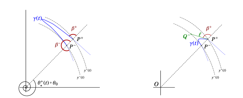
Figure 3. Left: The arc $\gamma(t)$. Right: the angles $\beta^{\pm}$

If $\phi:\gamma(t)\to\mathbb{R}$ is the tangent angle along the arc (i.e. $X_{s}={{\boldsymbol{E}}_{1}}(\phi)$), then the curvature integral is

$$\int_{\gamma(t)}\kappa\,ds=\phi_{P^{-}(t)}-\phi_{P^{+}(t)}.$$

The line segment $P^{+}P^{-}$ moves with angular velocity $\frac{d}{dt}\vartheta_{*}^{+}(t)$ and therefore adds area to the region enclosed by $\gamma(t)$ at the rate

$$\frac{1}{2}\Bigl{\{}\bigl{(}R_{j}^{+}\bigr{)}^{2}-\bigl{(}R_{j}^{-}\bigr{)}^{2}\Bigr{\}}\frac{d\vartheta_{*}^{+}(t)}{dt}$$

in which $R_{j}^{\pm}$ are evaluated at $\theta=\vartheta_{*}^{+}(t)+\theta_{0}$. Our construction of the cap implies that $\vartheta_{*}^{+}(t)=-t+o(1)$, and that this relation may be differentiated: $\frac{d}{dt}\vartheta_{*}^{+}(t)=-1+o(t)$.

The radii $R_{j}^{\pm}(\vartheta_{*}^{+}(t)+\theta_{0},t)$ are given in terms of their Yin-Yang coordinates $y^{\pm}(t)$ via

$$R_{j}^{\pm}(\vartheta_{*}^{+}(t)+\theta_{0},t)={\mathcal{R}}(\vartheta_{*}^{+}(t)+\theta_{0}-t+y^{\pm}).$$

It follows that at $\vartheta_{*}^{+}(t)+\theta_{0}$

$$\frac{1}{2}\Bigl{\{}\bigl{(}R_{j}^{+}\bigr{)}^{2}-\bigl{(}R_{j}^{-}\bigr{)}^{2}\Bigr{\}} =\frac{1}{2}\bigl{\{}{\mathcal{R}}(\vartheta_{*}^{+}(t)+\theta_{0}-t+y^{+})^{2}-{\mathcal{R}}(\vartheta_{*}^{+}(t)+\theta_{0}-t+y^{-})^{2}\bigr{\}}$$

$$={\mathcal{R}}\,{\mathcal{R}}^{\prime}\,(y^{+}-y^{-})$$

in which ${\mathcal{R}},{\mathcal{R}}^{\prime}$ are evaluated at $\vartheta_{*}(t)+\theta_{0}+\widetilde{y}$ for some $\widetilde{y}\in[y^{-},y^{+}]$ that is provided by the mean value theorem. The asymptotics of ${\mathcal{R}}$ imply that ${\mathcal{R}}{\mathcal{R}}^{\prime}=1+o(1)<2$. Our choice of $\theta_{0}$ was such that $0<y^{+}-y^{-}\leqslant\delta$. Hence

$$\left|\frac{1}{2}\Bigl{\{}\bigl{(}R_{j}^{+}\bigr{)}^{2}-\bigl{(}R_{j}^{-}\bigr{)}^{2}\Bigr{\}}\frac{d\vartheta_{*}^{+}(t)}{dt}\right|\leqslant 2\delta.$$

In total, the rate at which the area $A(t)$ enclosed by the arc $\gamma(t)$ grows is bounded by

$$\frac{dA}{dt}\leqslant-\bigl{(}\phi_{P^{-}(t)}-\phi_{P^{+}(t)}\bigr{)}+2\delta.$$

We estimate the change in tangent angle across the arc $\gamma(t)$. Let $\beta^{+}$ be the counterclockwise angle from the ray $\theta=\vartheta_{*}^{+}(t)+\theta_{0}$ to the tangent $X_{s}$ to $\gamma$ at $P^{+}$, and similarly, let $\beta^{-}$ be the counterclockwise angle from the same ray to the tangent to $\gamma$ at $P^{-}$ (see Figure 3). We have $0<\beta^{+}<\pi<\beta^{-}$ and $\phi_{P^{-}}-\phi_{P^{+}}=\beta^{-}-\beta^{+}$.

Recall that $\kappa-\langle X,X_{s}\rangle>0$ along ${\mathcal{C}}_{j}(t)$. Since $\kappa=\phi_{s}$ and $\langle X,X_{s}\rangle=\frac{1}{2}\frac{d}{ds}r^{2}$, where $r=\|X\|$, it follows that $\phi-\frac{1}{2}r^{2}$ increases as one traverses $\gamma$ from $P^{+}$ to $P^{-}$. Thus, at any point with polar coordinates $(\theta,r)$ on $\gamma$ one has

$$\phi>\phi_{P^{+}}+\frac{1}{2}(r^{2}-r_{P^{+}}^{2})$$

The lowest value $r$ has on $\gamma$ occurs at the point $P_{-}$, and we have just shown that $r_{P^{+}}^{2}-r_{P_{-}}^{2}\leqslant 2\delta$. Hence $\phi>\phi_{P^{+}}-2\delta$ on the entire arc $\gamma$.

It follows that if $\beta^{+}>\frac{3}{4}\pi$, then the angle between the tangent to $\gamma$ and the ray $OP^{+}$ ($O$ is the origin) will always be at least $\frac{3}{4}\pi-2\delta$, i.e. more than $\frac{5}{8}\pi$, provided we choose $\delta<\frac{\pi}{16}$.

Consider the line $\ell$ through $P^{+}$ whose angle with $OP^{+}$ is $\frac{5}{8}\pi$. The euclidean distance between $P^{-}$ and $P^{+}$ is $r_{P^{+}}-r_{P^{-}}\leqslant 2\delta/(r_{P^{-}}+r_{P^{+}})\leqslant C\delta|t|^{-1/2}$, since $r_{P^{+}}>r_{P^{-}}\gtrsim|t|^{1/2}$.

At this scale the Yin-Yang leaves will be almost straight lines near $P^{\pm}$, so that the line $\ell$ then intersects the Yin-Yang leaf with $y=y_{-}(t)$ at a point $Q^{-}(t)$, also at a distance $d(P^{-},Q^{-})\lesssim\delta|t|^{-1/2}$.

$$\vartheta_{j}^{+}(t)-\vartheta_{*}^{+}(t)-\theta_{0}\sim\frac{d(P^{-},Q^{-})}{r_{P^{-}}}\lesssim\delta|t|^{-1}\ll\theta_{0}.$$

Hence the largest polar angle on $\gamma$ will be at most

$$\vartheta_{j}^{+}(t)\leqslant\vartheta_{*}^{+}(t)+\theta_{0}+\delta|t|^{-1}\leqslant\vartheta_{*}^{+}(t)+2\theta_{0}.$$

Thus we find that if $|t|$ is sufficiently large, then either $\vartheta_{j}(t)<\vartheta_{*}(t)$, or else $\beta^{+}<\frac{5}{8}\pi$. In the latter case the area enclosed by $\gamma(t)$ decreases faster than

$$\frac{dA}{dt}\leqslant-\beta^{-}+\beta^{+}+2\delta\leqslant-\pi+\frac{5}{8}\pi+2\delta=-\frac{3}{8}\pi+2\delta<-\frac{\pi}{4},$$

again assuming that $\delta<\pi/16$.

We now finally prove that $\vartheta_{j}^{+}(t)-\vartheta_{*}^{+}(t)$ is uniformly bounded for all $t\in[-j,T]$ and $j$.

At $t=-j$ we have $\vartheta_{j}^{+}(t)<\vartheta_{*}^{+}(t)+\theta_{0}$, by definition of the initial curve ${\mathcal{C}}_{j}(-j)$. Hence, if at any time $t_{1}<T$ one has $\vartheta_{j}^{+}(t)>\vartheta_{*}^{+}(t)+2\theta_{0}$, then there is a largest interval $(t_{2},t_{3})\ni t_{1}$ on which $\vartheta_{j}^{+}(t)>\vartheta_{*}^{+}(t)+2\theta_{0}$. In particular, at $t=t_{2}$ one has $\vartheta_{j}^{+}(t)=\vartheta_{*}^{+}(t)+2\theta_{0}$.

Define the arc $\gamma(t)$ as above. Its enclosed area is at most $\varepsilon$, where we may assume that $\varepsilon<\pi/4$. During the time interval $(t_{2},t_{3})$ the area decreases at a rate of at least $\pi/4$, and therefore the length $t_{3}-t_{2}$ of the time interval cannot exceed $\varepsilon/(\pi/4)<1$. At time $t=t_{2}$ we had $\vartheta_{j}^{+}(t)=\vartheta_{*}^{+}(t)+2\theta_{0}$. Since $\vartheta_{j}^{+}(t),\vartheta_{*}^{+}(t)$ are nonincreasing functions, we have throughout $(t_{2},t_{3})$

$$\vartheta_{j}^{+}(t)-(\vartheta_{*}^{+}(t)+2\theta_{0}) \leqslant\vartheta_{j}^{+}(t_{2})-(\vartheta_{*}^{+}(t)+2\theta_{0})$$

$$=\vartheta_{*}^{+}(t_{2})+2\theta_{0}-(\vartheta_{*}^{+}(t)+2\theta_{0})$$

$$\leqslant\vartheta_{*}^{+}(t_{2})+2\theta_{0}-(\vartheta_{*}^{+}(t_{3})+2\theta_{0})$$

$$\leqslant\vartheta_{*}^{+}(t_{2})-\vartheta_{*}^{+}(t_{3}).$$

Since $\frac{d}{dt}\vartheta_{*}^{+}(t)=1+o(1)$ we find that

$$\vartheta_{j}^{+}(t)-(\vartheta_{*}^{+}(t)+2\theta_{0})\leqslant 1+o(1)<2$$

for all $t\in(t_{2},t_{3})$. ∎

To summarize, we can now decompose every very-old solution ${\mathcal{C}}_{j}(t)$, for $t\in[-T^{*}-1/2,-T^{*}]$ into four graphs in two different coordinate systems, $R_{j}^{\pm}(\theta,t)$ in polar coordinates, and $\Theta^{\pm}_{j}(y,t)$ in Yin-Yang polar coordinates.

Lemma 4.8 (Curvature bounds).

There exist $T<0$ such that for any $T^{\prime}<T$ the lengths $L_{j}(t)$ and curvatures of ${\mathcal{C}}_{j}(t)$ are uniformly bounded for all $j$ and all $t\in[T^{\prime},T-2]$.

Proof.

The length bounds follow from the fact that in $(y,\theta)$ coordinates each ${\mathcal{C}}_{j}(t)$ is contained in a uniformly bounded rectangle $|y|\leqslant\pi/2$, $-t\leqslant\theta\leqslant\vartheta_{*}^{+}(t)+2\theta_{0}+2$, and the fact that ${\mathcal{C}}_{j}(t)$ decomposes into four segments on each of which both $y$ and $\theta$ are monotone.

Consider a given value $T^{\prime}<T$. Assume that our Lemma fails, and that along some subsequence $j$ the maximal curvature of ${\mathcal{C}}_{j}(t)$ with $t\in[T^{\prime},T-2]$ becomes unbounded.

For $t\in[T^{\prime}-2,T]$ the lengths $L_{j}(t)$ of ${\mathcal{C}}_{j}(t)$ are uniformly bounded by some $L>0$. It follows that

$$\int_{T^{\prime}-2}^{T^{\prime}-1}\int_{{\mathcal{C}}_{j}(t)}\kappa^{2}\,ds\,dt=\bigl{[}-L_{j}(t)\bigr{]}_{T^{\prime}-2}^{T^{\prime}-1}<L.$$

Therefore, there is a sequence $t_{j}\in[T^{\prime}-2,T^{\prime}-1]$ such that

$$\int_{{\mathcal{C}}_{j}(t_{j})}\kappa^{2}\,ds<L.$$

By a Sobolev embedding theorem this implies that the curves ${\mathcal{C}}_{j}(t_{j})$ are uniformly $C^{1,1/2}$, i.e. they are continuously differentiable, and their tangent angles $\phi_{j}$ are uniformly Hölder continuous — in fact, for any two points at arclength coordinates $s_{1},s_{2}$ in ${\mathcal{C}}_{j}(t_{j})$ one has

$$|\phi(s_{2})-\phi(s_{1})|=\left|\int_{s_{1}}^{s_{2}}\kappa\,ds\right|\leqslant\sqrt{s_{2}-s_{1}}\sqrt{\int_{s_{1}}^{s_{2}}\kappa^{2}ds}\leqslant\sqrt{L}\sqrt{s_{2}-s_{1}}.$$

It follows that all ${\mathcal{C}}_{j}(t_{j})$ are uniformly locally Lipschitz curves. Now consider the solutions to curve shortening with ${\mathcal{C}}_{j}(t_{j})$ as initial data, i.e. consider $\widetilde{{\mathcal{C}}}_{j}(t)={\mathcal{C}}_{j}(t_{j}+t)$. These solutions all exist for $0\leqslant t\leqslant T-t_{j}\geqslant T-T^{\prime}$. Supposing that along some subsequence of $t_{j}$ the curvatures of the $\widetilde{{\mathcal{C}}}_{j}$ are not bounded for $1\leqslant t\leqslant T-T^{\prime}$, we pass to a further subsequence for which the initial curves $\widetilde{{\mathcal{C}}}_{j}(0)$ converge in $C^{1}$ to some limit curve $\widetilde{{\mathcal{C}}}_{*}$. The enclosed areas of the $\widetilde{{\mathcal{C}}}_{j}(0)$ then also converge, and hence, by Grayson’s theorem [6] the evolution by Curve Shortening ${\mathcal{C}}_{*}(t)$ starting from ${\mathcal{C}}_{*}$ exists for $0\leqslant t\leqslant T-T^{\prime}$. By continuous dependence on initial data it follows that the solutions $\widetilde{{\mathcal{C}}}_{j}(t)$ converge in $C^{\infty}$ to ${\mathcal{C}}_{*}(t)$ on any time interval $[\delta,T-T^{\prime}]$ with $\delta>0$. This implies that the curvatures of the $\widetilde{{\mathcal{C}}}_{j}(t)$ are uniformly bounded for $t\in[1,T-T^{\prime}]$, which then implies that the curvatures of ${\mathcal{C}}_{j}(t)$ are uniformly bounded after all for $t\in[t_{j}+1,t_{j}+T-T^{\prime}]\subset[T^{\prime},T-2]$. ∎

Appendix A The Yin-Yang Soliton

Hungerbühler and Smoczyk [8] proved uniqueness and existence of a rotating soliton for curve shortening that contains the origin. See also Halldorson [7] and Altschuler et.al. [1]. Here we derive its more detailed asymptotic behavior, which we use in our construction of the approximate solution.

A.1. The Yin–Yang soliton in polar coordinates

For an evolving family of curves written in polar coordinates $X(t,\theta)=r(t,\theta){{\boldsymbol{E}}_{1}}(\theta)$ the Curve Shortening Deficit is

$$(V-\kappa)\,ds=\left\langle X_{t}-\tfrac{X_{\theta\theta}}{\|X_{\theta}\|^{2}},JX_{\theta}\right\rangle d\theta=\Biggl{\{}-rr_{t}+\frac{r(r_{\theta\theta}-r)-2r_{\theta}^{2}}{r^{2}+r_{\theta}^{2}}\Biggr{\}}d\theta.$$

It follows that $X$ is a solution of CSF if and only if $r(\theta,t)$ satisfies

(A.1) $$r\frac{\partial r}{\partial t}=\frac{rr_{\theta\theta}-r_{\theta}^{2}}{r^{2}+r_{\theta}^{2}}-1=\frac{\partial}{\partial\theta}\Bigl{(}\arctan\frac{r_{\theta}}{r}\Bigr{)}-1.$$

If we look for solutions of the form $r(\theta,t)={\mathcal{R}}(\theta-t)$ we get an ODE for ${\mathcal{R}}(\theta)$

(A.2) $$-{\mathcal{R}}{\mathcal{R}}^{\prime}=\frac{{\mathcal{R}}{\mathcal{R}}^{\prime\prime}-{\mathcal{R}}^{\prime 2}}{{\mathcal{R}}^{2}+{\mathcal{R}}^{\prime 2}}-1.$$

Hungerbühler and Smoczyk [8] observed that this equation can be integrated once. By suitably rotating the curve around the origin we can ensure that the resulting integration constant vanishes, and we therefore have

(A.3) $$\frac{1}{2}{\mathcal{R}}(\theta)^{2}-\theta+\arctan\frac{{\mathcal{R}}^{\prime}(\theta)}{{\mathcal{R}}(\theta)}=0.$$

We consider the soliton that passes through the origin. When this happens ${\mathcal{R}}\to 0$ and ${\mathcal{R}}^{\prime}\to\infty$, so that (A.3) implies $\theta\to\pi/2$. The function ${\mathcal{R}}(\theta)$ is therefore defined for all $\theta>\pi/2$, and, as proved by Hungerbühler and Smoczyk, ${\mathcal{R}}^{\prime}(\theta)>0$ for all $\theta>\pi/2$.

A.2. Asymptotic expansion of ${\mathcal{R}}$

We now show that ${\mathcal{R}}(\theta)$ has an asymptotic expansion of the form

(A.4) $${\mathcal{R}}(\theta)=(2\theta)^{1/2}\left\{1+\frac{c_{1}}{2\theta}+\frac{c_{2}}{(2\theta)^{2}}+\cdots+\frac{c_{N}}{(2\theta)^{N}}+{\mathcal{O}}(\theta^{-N-1})\right\}\qquad(\theta\to\infty)$$

for any $N\in\mathbb{N}$. These expansions can be differentiated any number of times. The coefficients $c_{j}$ can be computed by substituting the expansions in (A.2) and recursively solving for $c_{j}$. In particular, one finds $c_{1}=0$, $c_{2}=-1$, and $c_{3}=\frac{11}{3}$ so that

(A.5) $${\mathcal{R}}(\theta) =\sqrt{2\theta}-\frac{1}{(2\theta)^{3/2}}+\frac{11}{3}\frac{1}{(2\theta)^{5/2}}+{\mathcal{O}}(\theta^{-7/2}) (\theta\to\infty)$$

(A.6) $${\mathcal{R}}^{\prime}(\theta) =\frac{1}{\sqrt{2\theta}}+\frac{3}{(2\theta)^{5/2}}-\frac{55}{3}\frac{1}{(2\theta)^{7/2}}+{\mathcal{O}}(\theta^{-9/2}) (\theta\to\infty).$$

This implies that the quantities $R=R(t)={\mathcal{R}}(-2t)$, $\varepsilon=1/R$, and $R_{\theta}=R_{\theta}(t)={\mathcal{R}}^{\prime}(-2t)$, which we use in the construction of the cap, have expansions in powers of $\tau=-4t$, given by

(A.7) $$\left\{\quad\begin{aligned} R={\mathcal{R}}(-2t)&=\sqrt{\tau}\bigl{\{}1-\tau^{-2}+\tfrac{11}{3}\tau^{-3}+{\mathcal{O}}(\tau^{-4})\bigr{\}}\\ \varepsilon=\frac{1}{R}&=\frac{1}{\sqrt{\tau}}\bigl{\{}1+\tau^{-2}-\tfrac{11}{3}\tau^{-3}+{\mathcal{O}}(\tau^{-4})\bigr{\}}.\\ R_{\theta}={\mathcal{R}}^{\prime}(-2t)&=\frac{1}{\sqrt{\tau}}\bigl{\{}1+3\tau^{-2}-\tfrac{55}{3}\tau^{-3}+{\mathcal{O}}(\tau^{-4})\bigr{\}}.\end{aligned}\right.$$

Proof of (A.4) Consider the quantity $u(\theta)=\theta-\tfrac{1}{2}{\mathcal{R}}(\theta)^{2}$. Since ${\mathcal{R}}^{\prime}(\theta)>0$ for all $\theta$ it follows from (A.3) that

(A.8) $$0<u(\theta)<\frac{\pi}{2}\text{ for all }\theta>\frac{\pi}{2}.$$

Directly differentiating $u=\theta-\frac{1}{2}{\mathcal{R}}^{2}$ and using (A.3) we find an equation for $u$,

(A.9) $$u^{\prime}(\theta)=1-2(\theta-u(\theta))\tan u(\theta).$$

i.e.

$$u^{\prime}+2\theta u=F(\theta,u){\stackrel{{\scriptstyle\textrm{def}}}{{=}}}1+2\theta(u-\tan u)+2u\tan u$$

We use induction to show that $u(\theta)$ has an expansion of the form

(A.10) $$u(\theta)=\frac{u_{1}}{\theta}+\frac{u_{2}}{\theta^{2}}+\cdots+\frac{u_{N}}{\theta^{N}}+{\mathcal{O}}(\theta^{-N-1})$$

for any $N\in\mathbb{N}$.

Begin with the case $N=0$. We know that $0<u<\pi/2<\theta$, so that $u<\tan u$, and hence

$$u^{\prime}(\theta)=1-2(\theta-u)\tan u\leqslant 1-2(\theta-u)u=1-2\theta u+2u^{2}$$

which implies

$$u^{\prime}+2\theta u\leqslant 1+2u^{2}\leqslant 1+\frac{\pi^{2}}{2}=C_{0}.$$

Multiply with $e^{\theta^{2}}$, and integrate

$$0<u(\theta)\leqslant u(\theta_{0})e^{\theta_{0}^{2}-\theta^{2}}+C_{0}\int_{\theta_{0}}^{\theta}e^{\xi^{2}-\theta^{2}}\,d\xi=O(\theta^{-1})\quad(\theta\to\infty),$$

Thus the case $N=0$ holds.

For the induction step we expand $\tan u$ in a Taylor series,

$$\tan u=u+\frac{u^{3}}{3}+\cdots=u+\sum_{k\geqslant 1}c_{k}u^{2k+1}$$

and rewrite the equation for $u$ as

$$F(\theta,u)=1+2u^{2}+\sum_{k\geqslant 1}2(\theta-u)c_{k}u^{2k+1}$$

Multiplying with $e^{\theta^{2}}$ and integrating from some fixed $\theta_{0}>\pi/2$ we get

(A.11) $$u(\theta)=e^{\theta_{0}^{2}-\theta^{2}}u(\theta_{0})+\int_{\theta_{0}}^{\theta}e^{\xi^{2}-\theta^{2}}F(\xi,u(\xi))\,d\xi$$

Repeated integration by parts leads to

(A.12) $$\int_{\theta_{0}}^{\theta}e^{\xi^{2}-\theta^{2}}\xi^{-k}d\xi=\\ \frac{1}{2}\theta^{-k-1}+\frac{k+1}{2}\theta^{-k-3}+\cdots+\frac{(k+1)\cdots(k+2m-1)}{2^{m}}\theta^{-k-2m-1}+{\mathcal{O}}(\theta^{-k-2m-3})$$

for all $k,m\in\mathbb{N}$. If we assume that $u$ has an expansion up to ${\mathcal{O}}(\theta^{-(N-1)})$, then we also have expansions for $u^{2}$ and $F(\theta,u)$ up to ${\mathcal{O}}(\theta^{-(N-1)})$. Substitute these expansions in the integral equation (A.11) and use (A.12) to conclude that $u$ has an expansion up to ${\mathcal{O}}(\theta^{-N})$, as claimed.

The expansion (A.10) for $u$, which we now have proved, implies ${\mathcal{R}}(\theta)=\sqrt{2(\theta-u(\theta))}$ also has an asymptotic expansion in powers of $\theta^{-1}$.

Finally, while one cannot in general differentiate asymptotic expansions, one can integrate them. Thus if a function $f(\theta)$ and its derivative $f^{\prime}(\theta)$ both have asymptotic expansions in powers of $\theta^{-1}$, then by integrating the expansion of $f^{\prime}$ one should get the expansion for $f$, up to a constant: this implies that the expansion of $f^{\prime}$ can be found by differentiating the expansion for $f$. We therefore only have to show that all derivatives of $u(\theta)$ have expansions in powers of $\theta^{-1}$, which will then imply that the expansions (A.10) can be differentiated.

To find expansions for $u^{(m)}$, note that if $u$ has an expansion with remainder ${\mathcal{O}}(\theta^{-N-1})$, then simple substitution in the differential equation (A.9) leads to an expansion for $u^{\prime}(\theta)$ with remainder ${\mathcal{O}}(\theta^{-N})$. Going further, one can differentiate (A.9) $m-1$ times and express $u^{(m)}(\theta)$ in terms of $u,u^{\prime},u^{\prime\prime},\dots,u^{(m-1)}$. This implies that if one has an expansion in powers of $\theta^{-1}$ of the first $m-1$ derivatives of $u$, then one also has an expansion for $u^{(m)}$. By induction it follows that all derivatives of $u$ have such expansions.

Similar arguments also apply to the expansions of ${\mathcal{R}}(\theta)$.

A.3. Inversion of the expansion of ${\mathcal{R}}$

The expansion (A.4), which expresses ${\mathcal{R}}$ as a function of $\theta$, implies that one can invert the function $\theta\mapsto{\mathcal{R}}(\theta)$, and that the inverse has an asymptotic expansion. It follows from (A.4) that

$${\mathcal{R}}(\theta)^{2}=(2\theta)\left\{1+\frac{\bar{c}_{1}}{2\theta}+\frac{\bar{c}_{2}}{(2\theta)^{2}}+\cdots+\frac{\bar{c}_{N}}{(2\theta)^{N}}+{\mathcal{O}}(\theta^{-N-1})\right\}$$

and hence

$$2\theta={\mathcal{R}}^{2}\left\{1+\frac{\bar{c}_{1}}{2\theta}+\frac{\bar{c}_{2}}{(2\theta)^{2}}+\cdots+\frac{\bar{c}_{N}}{(2\theta)^{N}}+{\mathcal{O}}(\theta^{-N-1})\right\}^{-1}.$$

Repeated substitution of this expansion in itself allows one to convert all powers of $(2\theta)$ on the left into powers of ${\mathcal{R}}^{2}$, so that we have an expansion

$$2\theta={\mathcal{R}}^{2}\left\{1+\frac{\widetilde{c}_{1}}{{\mathcal{R}}^{2}}+\frac{\widetilde{c}_{2}}{{\mathcal{R}}^{4}}+\cdots+\frac{\widetilde{c}_{N}}{{\mathcal{R}}^{2N}}+{\mathcal{O}}({\mathcal{R}}^{-2N-2})\right\}$$

for certain coefficients $\widetilde{c}_{i}$.

References

- [1] Dylan J. Altschuler, Steven J. Altschuler, Sigurd B. Angenent, and Lani F. Wu. The zoo of solitons for curve shortening in . Nonlinearity, 26(5):1189–1226, 2013.
- [2] Steven J. Altschuler and Matthew A. Grayson. Shortening space curves and flow through singularities. J. Differential Geom., 35(2):283–298, 1992.
- [3] Sigurd Angenent and Qian You. Ancient solutions to curve shortening with finite total curvature. Trans. Amer. Math. Soc., 374(2):863–880, 2021.
- [4] Jumageldi Charyyev. A compact non-convex ancient curve shortening flow, 2022. Preprint: arXiv:2204.05978.
- [5] Panagiota Daskalopoulos, Richard Hamilton, and Natasa Sesum. Classification of compact ancient solutions to the curve shortening flow. J. Differential Geom., 84(3):455–464, 2010.
- [6] Matthew A. Grayson. The heat equation shrinks embedded plane curves to round points. J. Differential Geom., 26:284–314, 1986.
- [7] Hoeskuldur P. Halldorsson. Self-similar solutions to the curve shortening flow. Trans. Amer. Math. Soc., 364(10):5285–5309, 2012.
- [8] N. Hungerbühler and K. Smoczyk. Soliton solutions for the mean curvature flow. Differential Integral Equations, 13(10-12):1321–1345, 2000.
- [9] Wikipedia contributors. Fermat’s spiral — Wikipedia, the free encyclopedia, 2021. https://en.wikipedia.org/w/index.php?title=Fermat%27s_spiral&oldid=1025901425 [accessed 2-July-2021].
- [10] Qian You. Some Ancient Solutions of Curve Shortening. PhD thesis, UW–Madison, December 2014.