Probing the Ellis-Bronnikov wormhole geometry
with a scalar field: clouds, waves and Q-balls

Abstract

The Ellis-Bronnikov solution provides a simple toy model for the study of various aspects of wormhole physics. In this work we solve the Klein-Gordon equation in this background and find an exact solution in terms of Heun’s function. This may describe ’scalar clouds’ ($i.e.$ localized, particle-like configuration) or scalar waves. However, in the former case, the radial derivative of the scalar field is discontinuous at the wormhole’s throat (except for the spherical case). This pathology is absent for a suitable scalar field self-interaction, and we provide evidence for the existence of spherically symmetric and spinning Q-balls in a Ellis-Bronnikov wormhole background.

1 Introduction

The study of (classical) solutions of a field theory in a given spacetime background is an important step towards various more complicated studies. For example, in the field quantization one starts usually with the field modes construction [1]; also, in black hole physics, a number of ’no-hair’ theorems can be established at the level of matter field equations, without the use of gravity equations [2], [3].

A particularly interesting type of spacetime geometry which is allowed by the Einstein’s field equations is provided by the (Lorentzian) traversable wormholes (WHs). These are ’topological handles’ connecting separated regions of a single Universe or “bridges” joining two different spacetimes. As such, they are (at least) interesting solutions of the General Relativity (with its various extensions), being a useful tool to probe the limits of the theory. The study of WHs started in with the work of Flamm in 1916 [4] together with the Einstein and Rosen paper in 1935 [5]. After several decades of (relatively) slow progress (see, however, Wheeler’s work [6], [7]), a fresh interest in the topic of WHs has been reawaken by the work of Morris and Thorne [8], the field branching off into diverse directions. Among other results, the work [8] has clarified that some form of exotic matter violating the energy conditions is necessary in order to keep the throat of the WH open.

One of the simplest (and an early) example of traversable WHs in General Relativity has been found in 1973 by Ellis [9] and Bronnikov [10]. This is a solution of the Einstein equations minimally coupled with a massless phantom scalar field ($i.e.$ with a wrong sign in front of its kinetic term). The Ellis-Bronnikov solution is an archetypal example of a WH geometry, with a large number of papers investigating its properties (here we mention only the results in [11] establishing that this configuration is unstable).

In the context of this study, the Ellis-Bronnikov geometry is of interest mainly because of its simple form, which allows for a more systematic study of the solutions of a field theory model. For simplicity, in this work we shall consider the simplest case of a massive scalar field, which may possess a self-interacting potential.

The initial motivation for this study came from this simple observation that removing a sphere from Minkowski spacetime allows for everywhere regular scalar multipoles, with a finite total mass. For concreteness, let us consider the Laplace equation for a static scalar field, $\nabla^{2}\Phi=0$. In flat spacetime, its general solution is described by a multipolar expansion, with $\Phi=\sum_{\ell,m}R_{\ell}(r)Y_{\ell}^{m}(\theta,\varphi)$, where $Y_{\ell}^{m}$ are spherical harmonics and $R_{\ell}(r)=c_{1}r^{\ell}+c_{2}/r^{\ell+1}$ ($(r,\theta,\varphi)$ being the usual spherical coordinates). Thus, any non-trivial solution diverges either at the origin or at infinity. However, the situation changes if we restrict the domain of existence of the field outside a sphere of radius $r_{B}$, and take $c_{1}=0$. Then any field mode is finite, with a nonzero total mass.

In some sense, a WH provides an explicit realization of this scenario; since the two sphere possesses a minimal nonzero size, and one can predict the existence in this case of scalar clouds ($i.e.$ particle-like, localized configurations with finite mass). Indeed, this is confirmed by the analysis in Section 3 of this paper, where we find closed form solutions of the Klein-Gordon equation in a Ellis-Bronnikov WH background which can be interpreted as ’scalar clouds’. However, they fail generically to satisfy the Klein-Gordon equation at the throat, with a discontinuity in the first radial derivative of the field, the only exception being the spherically symmetric configuration. Physically reasonable solutions are found to exist for scalar waves, only.

When turning on the scalar field self-interaction, we find in Section 4 that this cures the pathological behaviour of the scalar clouds at the throat. Focusing on a complex massive scalar field with quartic plus hexic self-interactions, we find numerical evidence is given for the existence of spherically symmetric and axially symmetric spinning Q-ball-type solutions in Ellis-Bronnikov WH background.

2 The model

We consider the action for a complex scalar field $\Phi$ with a self-interaction potential $U$

$$S=-\int\left[\frac{1}{2}g^{\mu\nu}\left(\Phi_{,\,\mu}^{*}\Phi_{,\,\nu}+\Phi_{,\,\nu}^{*}\Phi_{,\,\mu}\right)+U(\left|\Phi\right|)\right]\sqrt{-g}d^{4}x\ ,$$ (2.1)

where the asterisk denotes complex conjugation and $\Phi_{,\,{\mu}}={\partial\Phi}/{\partial x^{\mu}}$.

Variation of (2.1) with respect to the scalar field leads to the (non-linear) Klein-Gordon equation

$$\nabla^{2}\Phi=\frac{\partial U}{\partial\left|\Phi\right|^{2}}\Phi\ .$$ (2.2)

The stress-energy tensor $T_{\mu\nu}$ of the scalar field is

$$T_{\mu\nu}=\left(\Phi_{,\,\mu}^{*}\Phi_{,\,\nu}+\Phi_{,\,\nu}^{*}\Phi_{,\,\mu}\right)-g_{\mu\nu}\left[\frac{1}{2}g^{\alpha\beta}\left(\Phi_{,\,\alpha}^{*}\Phi_{,\,\beta}+\Phi_{,\,\beta}^{*}\Phi_{,\,\alpha}\right)+U(\left|\Phi\right|)\right]~{}.$$ (2.3)

In the above relations $g_{\mu\nu}$ is taken to be the metric tensor of the Ellis-Bronnikov solution, with the following parametrization

$$ds^{2}=dr^{2}+(r^{2}+r_{0}^{2})\left(d\theta^{2}+\sin^{2}\theta d\varphi^{2}\right)-dt^{2}~{},$$ (2.4)

$\theta$ and $\varphi$ being spherical coordinates with the usual range, while $r$ and $t$ are the radial and time coordinates, respectively. This geometry consists in two different regions $\Sigma_{\pm}$; the ‘up’ region ($\Sigma_{+}$) is found for $0<r<\infty$, while the ’down’ region ($\Sigma_{-}$) has $-\infty<r<0$. These regions are joined at $r=0$, which is the position of the spherical throat, which is a minimal surface of area $4\pi r_{0}^{2}$.

For the geometry (2.4), the equation (2.2) takes the form

$$\frac{\partial^{2}\Phi}{\partial r^{2}}+\frac{2r}{r^{2}+r_{0}^{2}}\frac{\partial\Phi}{\partial r}+\frac{1}{r^{2}+r_{0}^{2}}\left[\frac{\partial^{2}\Phi}{\partial\theta^{2}}+\cot\theta\frac{\partial\Phi}{\partial\theta}+\frac{1}{\sin^{2}\theta}\frac{\partial^{2}\Phi}{\partial\varphi^{2}}\right]-\frac{\partial^{2}\Phi}{\partial t^{2}}-\frac{\partial U}{\partial\left|\Phi\right|^{2}}\Phi=0.$$ (2.5)

The model is invariant under the global phase transformation $\Phi\to\Phi e^{i\alpha}$, leading to the conserved current

$$j^{\mu}=-i\left[(\Phi)^{*}\partial^{\mu}\Phi+\Phi\partial^{\mu}\Phi^{*}\right]\ ,\qquad\nabla_{\mu}j^{\mu}=0\ .$$ (2.6)

This implies the existence of a conserved Noether charge (corresponding to particle number), which is the integral of $j^{t}$ on spacelike slices,

$$Q_{\pm}=\int_{\Sigma_{\pm}}d^{3}x\sqrt{-g}~{}j^{t}.$$ (2.7)

Morover, for particle-like solutions (scalar clouds) one can assign a mass in both ’up’and ’down’ regions

$$E_{\pm}=-\int_{\Sigma_{\pm}}d^{3}x\sqrt{-g}~{}T_{t}^{t}.$$ (2.8)

One should note that these masses $E_{\pm}$ are assigned to the scalar field itself and they do not refer to the gravitational masses that can be computed for the Ellis-Bronnikov WH background in each asymptotic region.

3 The non-selfinteracting case

For the case of a massive scalar field with

$$U(\left|\Phi\right|)=\mu^{2}|\Phi|^{2},$$ (3.9)

(where $\mu\geq 0$ is the boson mass), one may separate the variables as

$$\Phi=R_{\ell}(r)Y_{\ell}^{m}(\theta,\varphi)e^{-i\omega t},$$ (3.10)

with $\omega$ the field frequency and $Y_{\ell}^{m}$ Laplace’s spherical harmonics (where $\ell\geq 0$ and $-\ell\leq m\leq\ell$). Then, after replacing in (2.5) one finds the following equation for the radial amplitude $R_{\ell}(r)$

$$\frac{1}{r^{2}+r_{0}^{2}}\frac{d}{dr}\left[(r^{2}+r_{0}^{2})\frac{dR_{\ell}}{dr}\right]+\left[\omega^{2}-\mu^{2}-\frac{\ell(\ell+1)}{r^{2}+r_{0}^{2}}\right]R_{\ell}=0~{}.$$ (3.11)

This equation possess an exact solution in terms of Heun confluent functions [12]

$$R_{\ell}(r)=c_{1}~{}H_{1}(r)+c_{2}~{}H_{2}(r)~{},$$ (3.12)

where

$$H_{1}(r)={\rm HeunC}\left[0,-\frac{1}{2},0,\frac{(\mu^{2}-\omega^{2})r_{0}^{2}}{4},\frac{(\omega^{2}-\mu^{2})r_{0}^{2}}{4}-\frac{\ell^{2}+\ell-1}{4},-\frac{r^{2}}{r_{0}^{2}}\right]~{},$$ (3.13)

$$H_{2}(r)=r_{~{}}{\rm HeunC}\left[0,\frac{1}{2},0,\frac{(\mu^{2}-\omega^{2})r_{0}^{2}}{4},\frac{(\omega^{2}-\mu^{2})r_{0}^{2}}{4}-\frac{\ell^{2}+\ell-1}{4},-\frac{r^{2}}{r_{0}^{2}}\right]~{},$$

$c_{1},c_{2}$ being arbitrary constants. Let us remarks that $H_{1}$, $H_{2}$ are an even and odd functions of $r$, respectively, such that in general $R_{\ell}$ has no definite parity.

Let us also remark that, with the change of function

$$R_{\ell}(r)=\frac{y(r)}{\sqrt{r^{2}+r_{0}^{2}}}~{},$$

the eq. (3.11) can be cast into a Schrodinger-like form

$$-\frac{d^{2}y}{dr^{2}}+V(r)y=(\omega^{2}-\mu^{2})y,~{}~{}~{}{\rm with}~{}~{}V(r)=\frac{1}{r^{2}+r_{0}^{2}}\bigg{(}\ell(\ell+1)-\frac{r_{0}^{2}}{r^{2}+r_{0}^{2}}\bigg{)}.$$

3.1 The $\omega^{2}=\mu^{2}$ limit

The ${\rm HeunC}$ function possesses a rather complicated expression; thus, to study the solutions’ properties we have used the software MAPLE, calculating series expansions and evaluating them numerically for various values of the parameters.

However, the solution (3.12) greatly simplifies for $\omega^{2}=\mu^{2}$, a case which captures also the basic properties of the solutions with $\omega^{2}<\mu^{2}$. The radial amplitude in this case reads

$$R_{\ell}(r)=c_{1}{\rm L}_{P}(\ell,ir/r_{0})+c_{2}{\rm L}_{Q}(\ell,ir/r_{0})~{},$$ (3.14)

where ${\rm L}_{P}$ and ${\rm L}_{Q}$ are Legendre functions of first and second kind respectively, the explicit form for the first values of $\ell$ being

$$R_{0}(r)=c_{1}+c_{2}\arctan(\frac{r}{r_{0}}),~{}~{}R_{1}(r)=c_{1}\frac{r}{r_{0}}+c_{2}(\frac{r}{r_{0}}\arctan(\frac{r}{r_{0}})+1),$$

$$R_{2}(r)=c_{1}(\frac{1}{3}+\frac{r^{2}}{r_{0}^{2}})+c_{2}\left((\frac{1}{3}+\frac{r^{2}}{r_{0}^{2}})\arctan(\frac{r}{r_{0}})+\frac{r}{r_{0}}\right),~{}~{}$$ (3.15)

$$R_{3}(r)=c_{1}(\frac{r}{r_{0}}+\frac{5r^{3}}{3r_{0}^{3}})+c_{2}\left((\frac{r}{r_{0}}+\frac{5r^{3}}{3r_{0}^{3}})\arctan(\frac{r}{r_{0}})+\frac{5r^{2}}{3r_{0}^{2}}+\frac{4}{9}\right)~{}.$$

We are interested in localized, particle-like solutions, with a radial amplitude which is $continuous$ and $finite$ everywhere (in particular as $r\to\pm\infty)$. These requirements are satisfied by the $\ell=0$ mode, the radial profile $R_{0}(r)$ approaching constant values on each asymptotic region of the wormhole. However, one can see that for $\ell\geq 1$ the solution necessarily diverges as $r\to\infty$ or as $r\to-\infty$. Let us exemplify this for $\ell=1$, in which case

$$R_{1}\to(2c_{1}+c_{2}\pi)\frac{r}{2r_{0}}+O(1/r^{2})~{}~{}{\rm as}~{}r\to\infty,~{}~{}{\rm and}~{}~{}R_{1}\to(-2c_{1}+c_{2}\pi)\frac{r}{2r_{0}}+O(1/r^{2})~{}~{}{\rm as}~{}r\to-\infty.$$ (3.16)

The only way to cure this pathology is to consider $R_{1}$ to be the union of two separate solutions, $R_{1}^{(+)}(r)$ valid for $r\geq 0$ (with $R_{1}^{(+)}\to 0$ as $r\to\infty$), and $R_{1}^{(-)}(r)$ (with $r\leq 0$ and $R_{1}^{(-)}\to 0$ as $r\to-\infty$), which are joined at $r=0$. That is for $R_{1}^{(+)}(r)$ one takes $c_{1}=-c_{2}\pi/2$, while for $R_{1}^{(-)}(r)$ the choice is $c_{1}=c_{2}\pi/2$. This results in

$$R_{1}^{(+)}(r)=1+\frac{r}{r_{0}}\left(\arctan(\frac{r}{r_{0}})-\frac{\pi}{2}\right),~{}~{}R_{1}^{(-)}(r)=1+\frac{r}{r_{0}}\left(\arctan(\frac{r}{r_{0}})+\frac{\pi}{2}\right),~{}~{}$$ (3.17)

The total mass of this solution is $E_{\pm}=\pi^{2}r_{0}/3$.

The same procedure works for any value of $\ell$, and one finds with the following generic expression

$$R_{\ell}^{(+)}(r)=f_{\ell}(r)+g_{\ell}(r)\left(\arctan(\frac{r}{r_{0}})-\frac{\pi}{2}\right),~{}~{}R_{\ell}^{(-)}(r)=(-1)^{\ell+1}\left(f_{\ell}(r)+g_{\ell}(r)\left(\arctan(\frac{r}{r_{0}})+\frac{\pi}{2}\right)\right)$$ (3.18)

where $f_{\ell}(-r)=(-1)^{\ell+1}f_{\ell}(r),$ $g_{\ell}(-r)=(-1)^{\ell}g_{\ell}(r).$ such that $R_{\ell}^{(+)}(r)=R_{\ell}^{(-)}(-r)$. The functions $f_{\ell}$, $g_{\ell}$ are polynomials, with

$$\ell=2k:~{}~{}f_{\ell}(r)=\sum_{j=0}^{k-1}c_{j}(\frac{r}{r_{0}})^{2j+1},~{}~{}g_{\ell}(r)=\sum_{j=0}^{k}\bar{c}_{j}(\frac{r}{r_{0}})^{2j},$$ (3.19)

$$\ell=2k+1:~{}~{}f_{\ell}(r)=\sum_{j=0}^{k}d_{j}(\frac{r}{r_{0}})^{2j},~{}~{}g_{\ell}(r)=\sum_{j=0}^{k}\bar{d}_{j}(\frac{r}{r_{0}})^{2j+1},$$ (3.20)

where $k=0,1,\dots$ and $c_{j},\bar{c}_{j},d_{j},\bar{d}_{j}$ real coefficients.

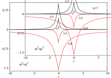
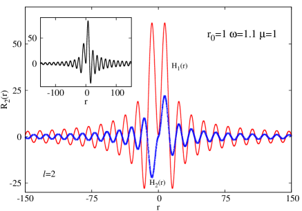
Figure 1: Left panel: The profiles of the $\ell=0,1,2,3,4$ radial amplitudes (3.18) with $\omega^{2}=\mu^{2}$. Right panel: A wave-like solution is shown for a $\ell=2$ configuration with $c_{1}=1$, $c_{2}=0$ ($H_{1}(r)$) and $c_{1}=0$, $c_{2}=0.9$ ($H_{2}(r)$) in the near-throat expansion (3.24). The inset shows the general solution.

One finds $e.g.$

$$f_{0}=0,~{}f_{1}=1,~{}f_{2}=\frac{r}{r_{0}},~{}f_{3}=\frac{4}{9}+\frac{5r^{2}}{3r_{0}^{2}},~{}f_{4}=\frac{55r}{9r_{0}}+\frac{35r^{3}}{3r_{0}^{3}},~{}f_{5}=\frac{64}{225}+\frac{49r^{2}}{15r_{0}^{2}}+\frac{21r^{4}}{5r_{0}^{4}},~{}$$ (3.21)

$$g_{0}=1,~{}g_{1}=\frac{r}{r_{0}},~{}g_{2}=\frac{1}{3}+\frac{r^{2}}{r_{0}^{2}},~{}g_{3}=\frac{r}{r_{0}}+\frac{5r^{3}}{3r_{0}^{3}},~{}g_{4}=1+\frac{10r^{2}}{3r_{0}^{2}}+\frac{35r^{4}}{3r_{0}^{4}},~{}g_{5}=1+\frac{r}{r}+\frac{14r^{3}}{3r_{0}^{3}}+\frac{21r^{5}}{5r_{0}^{5}},~{}$$

The profile of the first four radial amplitudes are shown in Fig. (1) (left panel).

However, the solution above is not fully satisfactory, since the derivatives of $R_{\ell}^{(+)}$ and $R_{\ell}^{(-)}$ do not match at the throat (although $R_{\ell}^{(+)}(0)=R_{\ell}^{(-)}(0)$). One finds $e.g.$ $\frac{dR_{0}^{(+)}}{dr}\big{|}_{r=0^{+}}=-\frac{dR_{0}^{(-)}}{dr}\big{|}_{r=0^{-}}=\frac{1}{r_{0}},$ $\frac{dR_{1}^{(+)}}{dr}\big{|}_{r=0^{+}}=-\frac{dR_{1}^{(-)}}{dr}\big{|}_{r=0^{-}}=-\frac{\pi}{2r_{0}},$ and $\frac{dR_{2}^{(+)}}{dr}\big{|}_{r=0^{+}}=-\frac{dR_{2}^{(-)}}{dr}\big{|}_{r=0^{-}}=\frac{4}{3r_{0}}.$ That is, the Klein-Gordon equation fails to be satisfied at the throat.

The only exception here is the $\ell=0$ mode, where the generic solution in (3.15) (with the same choice for $c_{1}$, $c_{2}$ for all range of $r$) has smooth derivatives at the throat, and approaches a constant nonzero value at least in one of the asymptotic regions, with $R_{0}\to c_{1}+c_{2}\frac{\pi}{2}+O(1/r)$ as $r\to\infty$, and $R_{0}\to c_{1}-c_{2}\frac{\pi}{2}+O(1/r)$ as $r\to-\infty$. One remarks that this radial function cannot vanish in both asymptotic regions. The case of a $\ell=0$ solution with $R_{0}\to 0$ as $r\to\pm\infty$ is contained in the general expression (3.18) (see also Figure 1). However, then the first derivative of $R_{0}$ is discontinuous at $r=0$.

3.2 The general case

Let us start with configurations satisfying the bound state condition $\omega^{2}<\mu^{2}$, in which case on may expect the existence of smooth scalar clouds. However, we have found that all properties of the $\ell>0$ solutions discussed above hold also on this case. The emerging picture can be summarized as follows. When fixing the constants $c_{1}$ and $c_{2}$, both functions $H_{1}$ and $H_{2}$ in the general solution (3.12) diverge for $|r|\to\infty$ and generic values of the parameters. However, it is possible to fine tune $c_{1}$, $c_{2}$ to get the solutions going to zero as $r\to\infty$, but then they are divergent as $r\to-\infty$ (or viceversa). In this case, the solutions are smooth at the throat, in particular with $R_{\ell}(0^{+})=R_{\ell}(0^{-})$.

As with the solutions in Section 3.1, it is possible to construct a solution $R_{\ell}$ which goes to zero as $r\to\pm\infty$, by choosing a different relation between $c_{1}$ and $c_{2}$ for each sign of $r$. However, then a discontinuous derivative of $R_{\ell}$ is unavoidable at $r=0$.

The absence of smooth $C^{1}$ solutions with $\omega^{2}<\mu^{2}$ can be seen from the following simple argument, which does not require an explicit form of the solution. After multiplying the eq. (3.11) with $R_{\ell}$, rearranging and integrating it, one finds that the solutions should satisfy the following identity:

$$(r^{2}+r_{0}^{2})R_{\ell}\frac{dR_{\ell}}{dr}\bigg{|}_{-\infty}^{\infty}=\int_{-\infty}^{\infty}dr\left[(r^{2}+r_{0}^{2})\left(\frac{dR_{\ell}}{dr}\right)^{2}+\left((r^{2}+r_{0}^{2})(\mu^{2}-\omega^{2})+{\ell(\ell+1)}\right)R_{\ell}^{2}\right].$$ (3.23)

The $l.h.s.$ vanishes identically (since $R_{\ell}\sim e^{-\sqrt{\mu^{2}-\omega^{2}}|r|}/|r|$ as $r\to|\infty|$); however, for $\omega^{2}<\mu^{2}$ the $r.h.s.$ is strictly positive. Thus we conclude the absence of physically reasonable scalar clouds in a Ellis-Bronnikov background (note that for $\omega\neq 0$ this holds also for the $\ell=0$ mode).

The picture is rather different for $\omega^{2}>\mu^{2}$, in which case the solution is a smooth wave-like function. The asymptotic analysis reveals that the radial amplitude tends to zero as $|r\to\infty|$, with the following far field regime behaviour $R_{\ell}\sim\frac{1}{|r|}(a_{1}\cos{\sqrt{\omega^{2}-\mu^{2}}r}+a_{2}\sin{\sqrt{\omega^{2}-\mu^{2}}r})$. At the throat, the solution possesses a power series expansion, the first term being

$$R_{\ell}(r)=c_{1}\left(1+\left(\frac{1}{2}(\mu^{2}-\omega^{2})+\frac{\ell(\ell+1)}{2r_{0}^{2}}\right)r^{2}+\dots\right)+c_{2}\left(r+\left(\frac{1}{4}(\mu^{2}-\omega^{2})+\frac{(\ell-1)(\ell+2)}{4r_{0}^{2}}\right)r^{3}+\dots\right)~{}~{}.~{}{~{}~{}}$$ (3.24)

The profile of typical wave-like radial amplitudes is shown in Figure 1 (right panel). In particular, one can notice that $H_{1}$ and $H_{2}$ are even and odd functions of $r$, respectively. The inset there shows the general solution (the sum of $H_{1}$ and $H_{2}$), which possesses no parity.

4 A self-interacting scalar field: Q-balls in Ellis-Bronnikov

One may ask if the non-smooth behavior found for clouds in the previous Section can be cured by turning on the scalar field self-interaction. The answer is positive, as shown by the existence of the following exact solution for a static, spherically symmetric real scalar field with a sextic potential

$$\Phi=\frac{c_{0}}{\sqrt{r^{2}+r_{0}^{2}}},~{}~{}~{}U(\Phi)=\beta\Phi^{6},~{}~{}{\rm where}~{}~{}\beta=-\frac{r_{0}^{2}}{3c_{0}^{4}}.$$ (4.26)

This describes a smooth, even-parity configuration (with $\Phi^{\prime}(0)=0)$, possessing a finite mass $E_{\pm}=\frac{2c_{0}^{2}\pi^{2}}{3r_{0}}$. However, this solution does not seem to possess generalizations with nonzero $\omega$ and $\mu$.

Therefore, to better understand the issue of non-linear clouds in a WH background, we shall consider for the rest of this Section a more complicated scalar potential with quadratic, quartic and sextic terms

$$U(|\Phi|)=\mu^{2}|\Phi|^{2}-\lambda|\Phi|^{4}+\beta|\Phi|^{6}.$$ (4.27)

with $\lambda,\beta$ positive constants. As discussed for the first time by Coleman in Ref. [14], this potential allows for nontopological soliton solutions in a flat spacetime background –the Q-balls. Such configurations have a rich structure and found a variety of physically interesting applications, see $e.g.$ the review work [15], [16]. Here we shall focus on the simplest Q-balls, corresponding to spherically symmetric and spinning (even parity) configurations, and show that the known flat space solutions possess generalizations in a Ellis-Bronnikov WH background. Moreover, as expected, the nonlinearities cure the pathological behaviour of the scalar field at the throat, leading to smooth, finite mass solutions.

Also, following the usual conventions in the literature, the numerical solutions reported here have been found for the following parameters in the potential (4.27))

$$\mu^{2}=1,~{}~{}\lambda=2,~{}~{}\beta=1.$$ (4.28)

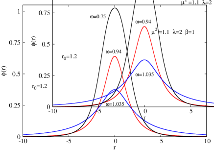
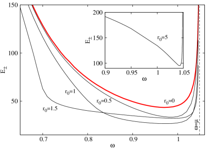
Figure 2: Left panel: The profile of typical spherical Q-balls. Right panel: The mass-frequency diagram is shown for spherical Q-balls with several values of the throat radius $r_{0}$.

4.1 Spherically symmetric Q-balls

The simplest Q-balls are spherically symmetric, with a scalar field Ansatz

$$\Phi=\phi(r)e^{-i\omega t}~{},$$ (4.29)

where $\phi(r)$ is a real field amplitude (which is an even function of $r$, such that $E_{+}=E_{-}$), and $\omega>0$ is the frequency. Close to the throat, one finds the following approximate solution,

$$\phi(r)=\phi_{0}+\phi_{2}r^{2}+\dots,~{}~{}{\rm where}~{}~{}\phi_{2}=\frac{1}{2}\phi_{0}(3\phi_{0}^{4}-2\phi_{0}^{2}\lambda+\mu^{2}-\omega^{2}),$$ (4.30)

(note that no discontinuities occur at $r=0$), while the field vanishes asymptotically, $\phi\sim c_{0}e^{-\sqrt{\mu^{2}-\omega^{2}}|r|}/|r|$.

The solutions connecting the above asymptotics are found numerically, the equation for $\phi(r)$ being solved by using a standard Runge-Kutta solver and implementing a shooting method. Some results of the numerical integration are shown in Figure (2). In the left panel we display the profile of the radial amplitude for several frequencies (keeping fixed other parameters of the problem). The frequency-mass diagram is shown in the right panel, for several values of the throat parameter $r_{0}$. One can see that the picture found for a Minkowski spacetime background is generic, the solutions existing for finite range of frequencies, $\omega_{min}<\omega<\mu$. At the ends of this interval, the mass $E$ increases without bounds. A similar behavior is found for the Noether charge $Q$.

It is the non-linear self-interaction which circumvents the non-existence result (3.23) (with $\ell=0$ and $R_{0}\equiv\phi$). Although the $l.h.s.$ there still vanishes for Q-balls, the term $(\mu^{2}-\omega^{2})\phi^{2}$ on the $r.h.s.$ of that equation is replaced with $(\mu^{2}-\omega^{2})\phi^{2}-2\lambda\phi^{4}+3\beta\phi^{6}$, which has no definite sign (and in fact takes negative values for some range of $r$). Also, following the standard scaling arguments in the literature [18], [19], one can show that these solutions satisfy the virial identity

$$\int_{-\infty}^{\infty}dr\left[(r^{2}-2rr_{0}-r_{0}^{2})\phi^{\prime 2}+(3r^{2}-2rr_{0}+r_{0}^{2})(U(\phi)-\omega^{2})\right]=0.$$ (4.31)

One can see that, different from the flat spacetime case, the $r$-factor in front of the kinetic term becomes negative for small enough $r$. This relation has been used as a further test of numerical accuracy.

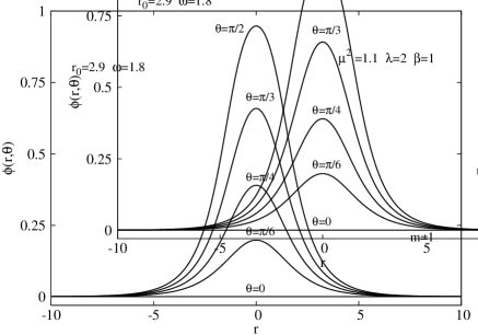
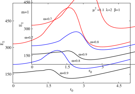
Figure 3: Left panel: The scalar amplitude of a typical spinning Q-ball is shown for several angular values. Right panel: The mass-frequency diagram is shown for spinning Q-balls with several values of the throat radius $r_{0}$.

4.2 Spinning Q-balls

Solutions with a non-zero angular momentum exist as well, they being found for a scalar field ansatz

$$\Phi=\phi(r,\theta)e^{i(m\varphi-\omega t)}~{},$$ (4.32)

where $\phi$ is a real function and $m=\pm 1,\pm 2\dots$ is the azimuthal harmonic index. Note that the $(t,\varphi)$-dependence of $\Phi$ occurs as a phase factor only, such that the energy-momentum tensor depends on $(r,\theta)$, only (however, $m$ and $\omega$ still enter the expression of $T_{\mu\nu}$). These solutions possess a nonzero angular momentum density $T_{\varphi}^{t}=2m\omega\phi^{2}=mj^{t}$, and a total angular momentum

$$J_{\pm}=\int_{\Sigma_{\pm}}d^{3}x\sqrt{-g}~{}T_{\varphi}^{t}.$$ (4.33)

Interestingly, the proportionality between angular momentum and Noether charge found for a Minkowski spacetime background [20], [21] still holds for a WH background,

$$J_{\pm}=mQ_{\pm},$$ (4.34)

such that angular momentum is still quantized.

With the ansatz ((2.4), (4.32), the Klein-Gordon equation (2.2) reduces to

$$\phi_{,rr}+\frac{1}{r^{2}+r_{0}^{2}}\left(\phi_{,\theta\theta}+2r\phi_{,r}+\cot\theta\phi_{,\theta}-\frac{m^{2}}{\sin^{2}\theta}\phi\right)-(\mu^{2}-\omega^{2}-2\lambda\phi^{2}+3\beta\phi^{4})\phi=0$$ (4.35)

We are interested in localized, particle-like solutions of this equation, with a finite scalar amplitude $\phi$ and a regular energy density distribution. In our approach, $Q$-clouds are found by solving the equation (2.5) with suitable boundary conditions, by using a professional package, based on the iterative Newton-Raphson method [22], the input parameters being $\{\omega,m;\mu,\lambda,\beta\}$. The mass-energy and angular momentum are computed from the numerical output. The boundary conditions result from the study of the solutions on the boundary of the integration domain. The scalar field vanishes as $|r|\to\infty$, while the existence of a bound state requires $\omega<\mu$. Also, the regularity of solutions impose that the scalar field vanishes on the symmetry axis ($\theta=0,\pi$). This behavior holds also in the flat spacetime limit; however, the boundary conditions at $r=0$ are different. While in Minkowski spacetime the scalar field vanishes at the origin (as imposed by the finiteness of various physical quantities), the condition for a WH is $\partial_{r}\phi|_{r=0}=0$, while the field does not vanish at the throat. As such, the configurations possess a reflection symmetry $w.r.t.$ to the throat, $\phi(-r)=\phi(r)$ and $E_{+}=E_{-}$, $J_{+}=J_{-}$.

We restrict our study to configurations which are invariant under a reflection in the equatorial plane $\theta=\pi/2$. Also, we shall restrict our study to configuration whose scalar amplitude $\phi(r,\theta)$ has no nodes.

The profile of a typical solution is displayed in Figure 3 (left panel), where the field amplitude $\phi$ is shown as a function of $r$ for several values of the polar angle $\theta$. The $\omega$-dependence of solutions’ mass is qualitatively similar with that found in the spherically symmetric case, and we shall not exhibit it here. We plot instead the mass dependence on the throat parameter $r_{0}$ for several values of the field frequency. One can see that, rather counter-intuitive, this dependence is non-monotonic, with the existence of local extrema.

5 Further remarks. Conclusions

For a wormhole (WH) geometry, a two sphere possesses a minimal nonzero size, which connects two asymptotically flat regions. This property suggest that the usual $r=0$ divergence of the solutions of a (linear) field theory model are absent in this case. The main purpose of this paper was to investigate this aspect for the simplest case of a scalar field and a Ellis-Bronnikov wormhole geometry.

Our results can be summarized as follows. For a free complex massive scalar field, the Klein-Gordon equation has a general exact solution that can be expressed in terms of Heun’s functions, with two distinct classes of configurations. For $\omega^{2}>\mu^{2}$ (with $\omega$ and $\mu$ the field’s frequency and mass, respectively), one finds wave-like solutions, which propagates from one asymptotic region to another, being smooth everywhere. The solutions with $\omega^{2}\leq\mu^{2}$ are ’scalar clouds’, the field amplitude vanishing asymptotically. However, the Klein-Gordon equation fails to be satisfied at the throat, with a discontinuity in the radial derivative of the scalar field. The only exception is found for the spherically symmetric mode with $\omega^{2}=\mu^{2}$, which, in fact, has the same functional dependence on the radial coordinate as the phantom field that sources the Ellis-Bronnikov solution [9], [10]. The pathological behaviour of the $\ell>0$ scalar clouds strongly suggest the absence of multipolar deformation of the Ellis-Bronnikov WH, and can be viewed as a ’no-hair’ theorem.

In the second part of this work we addressed the question on how the field’s non-linearities may cure the scalar clouds’ pathology found in the linear model. Considering a specific self-interacting potential which in flat spacetime allows for particle-like solutions (the Q-balls), we have provided numerical evidence for the existence of smooth solitonic configurations in a Ellis-Bronnikov WH background. Two different classes of solutions have been considered, corresponding to spherically symmetric and axially symmetric spinning configurations which are invariant $w.r.t.$ a reflection in the equatorial plane. However, negative parity solutions should also exist, their flat space limit being considered in [20], [23]. Also, on general grounds we predict the existence of a general tower of solutions (Q-ball ’chains’ and ’molecules’ [24]) corresponding to regularized versions of the generic $(\ell,m,w)$-scalar clouds discussed in Section 3.1.

Another interesting question concerns the generality of the results reported in this work. Although a systematic work is clearly necessary, we expect some of the qualitative results reported above to hold for a generic spherically symmetric WH, in particular those found for linear waves and $Q$-balls.

References

- [1] N. D. Birrell and P. C. W. Davies, Quantum Fields in Curved Space, Cambridge Monographs on Mathematical Physics (Cambridge Univ. Press, Cambridge, UK, 1984).
- [2] J. D. Bekenstein, Black hole hair: 25 - years after, [gr-qc/9605059].
- [3] C. A. R. Herdeiro and E. Radu, Int. J. Mod. Phys. D 24 (2015) no.09, 1542014 [arXiv:1504.08209 [gr-qc]].
- [4] L. Flamm, Phys.Z. 17 (1916) 448.
- [5] A. Einstein and N. Rosen, Phys. Rev. 48 (1935) 73.
- [6] J. A. Wheeler, Annals Phys. 2 (1957), 604-614
- [7] J. A. Wheeler, Geometrodynamics (Academic, New York, 1962).
- [8] M. S. Morris and K. S. Thorne, Am. J. Phys. 56, 395 (1988).
- [9] H. G. Ellis, J. Math. Phys. 14, 104 (1973)
- [10] K. A. Bronnikov, Acta Phys. Polon. B 4, 251 (1973).
-
[11]
J. A. Gonzalez, F. S. Guzman and O. Sarbach,
Class. Quant. Grav. 26 (2009), 015010
[arXiv:0806.0608 [gr-qc]];
J. A. Gonzalez, F. S. Guzman and O. Sarbach, Class. Quant. Grav. 26 (2009), 015011 [arXiv:0806.1370 [gr-qc]].
J. L. Blázquez-Salcedo, X. Y. Chew and J. Kunz, Phys. Rev. D 98 (2018), 044035 [arXiv:1806.03282 [gr-qc]]. -
[12]
A. Ronveaux,
Heun’s differential equations,
Oxford Science Publications
(The Clarendon Press Oxford University Press,1995).
S. Yu. Slavianov and W. Lay, Special Functions: A Unified Theory Based on Singularities, Oxford University Press (2000). - [13] P. Kanti, B. Kleihaus and J. Kunz, Phys. Rev. D 85 (2012), 044007 [arXiv:1111.4049 [hep-th]].
- [14] S. R. Coleman, Nucl. Phys. B 262 (1985) 263 [Erratum-ibid. B 269 (1986) 744].
- [15] E. Radu and M. S. Volkov, Phys. Rept. 468 (2008) 101 [arXiv:0804.1357 [hep-th]].
- [16] Y. M. Shnir, ’Topological and Non-Topological Solitons in Scalar Field Theories’, Cambridge University Press, 2018.
- [17] V. Dzhunushaliev, V. Folomeev, C. Hoffmann, B. Kleihaus and J. Kunz, Phys. Rev. D 90 (2014) no.12, 124038 [arXiv:1409.6978 [gr-qc]].
- [18] G. H. Derrick, J. Math. Phys. 5 (1964), 1252-1254
- [19] C. A. R. Herdeiro, J. M. S. Oliveira, A. M. Pombo and E. Radu, [arXiv:2109.05027 [gr-qc]].
- [20] M. S. Volkov and E. Wohnert, Phys. Rev. D 66 (2002) 085003 [hep-th/0205157].
- [21] B. Kleihaus, J. Kunz and M. List, Phys. Rev. D 72 (2005) 064002 [gr-qc/0505143].
-
[22]
W. Schönauer and R. Weiß,
J. Comput. Appl. Math. 27, 279 (1989) 279;
M. Schauder, R. Weiß and W. Schönauer, The CADSOL Program Package, Universität Karlsruhe, Interner Bericht Nr. 46/92 (1992). - [23] B. Kleihaus, J. Kunz, M. List and I. Schaffer, Phys. Rev. D 77 (2008) 064025 [arXiv:0712.3742 [gr-qc]].
-
[24]
C. A. R. Herdeiro, J. Kunz, I. Perapechka, E. Radu and Y. Shnir,
Phys. Lett. B 812 (2021), 136027
[arXiv:2008.10608 [gr-qc]];
C. A. R. Herdeiro, J. Kunz, I. Perapechka, E. Radu and Y. Shnir, Phys. Rev. D 103 (2021) no.6, 065009 [arXiv:2101.06442 [gr-qc]].