Time-Adaptive Recurrent Neural Networks

Abstract

Data are often sampled irregularly in time. Dealing with this using Recurrent Neural Networks (RNNs) traditionally involved ignoring the fact, feeding the time differences as additional inputs, or resampling the data. All these methods have their shortcomings. We propose an elegant alternative approach where instead the RNN is in effect resampled in time to match the time of the data. We use Echo State Network (ESN) and Gated Recurrent Unit (GRU) as the basis for our solution. Such RNNs can be seen as discretizations of continuous-time dynamical systems, which gives a solid theoretical ground for our approach. Similar recent observations have been made in feed-forward neural networks as neural ordinary differential equations. Our Time-Adaptive ESN (TAESN) and GRU (TAGRU) models allow for a direct model time setting and require no additional training, parameter tuning, or computation compared to the regular counterparts, thus retaining their original efficiency. We confirm empirically that our models can effectively compensate for the time-non-uniformity of the data and demonstrate that they compare favorably to data resampling, classical RNN methods, and alternative RNN models proposed to deal with time irregularities on several real-world nonuniform-time datasets.

1 Introduction

A usual assumption when applying Recurrent Neural Networks (RNNs) is that the time series is uniformly sampled in time. In reality, however, this is often not the case because of multiple reasons: data is gathered at irregular intervals, like patient examinations, expeditions; data comes from sources that get dated, like archaeological or geological samples, historical written sources; the data is recorded when a certain event happens, like an action by a user, an accident, a natural phenomenon, economic transaction; neural spike signals, etc. Here we deal with the case when the time irregularities are known, i.e., data samples have time stamps. Missing values in time series can also be treated as time-irregularity, as long as the data are missing in all input dimensions at the same time.

When data is irregularly sampled in time, typically RNNs are not applied, the time irregularity is ignored, the data are resampled by interpolation, or the time irregularities are simply fed as additional inputs in hopes that the model will learn to properly deal with them. All these approaches have their limitations.

Several specialized RNN architectures have been proposed recently to address this problem. They typically treat time irregularities as a special kind of input aiming in learning to accommodate it better. We review them and other alternatives in Section 2.

Here we take a bit different approach. Many types of RNNs can be seen as discretizations of continuous-time dynamical systems. Based on this, we can re-discretize them with variable time steps that can be adapted to match the ones in the data. This way, since time is relative, we make RNNs “live” in the time of the data, as opposed to resample the data to match the regular time of RNNs. We investigate this in two instances of RNNs: echo state networks and gated recurrent units.

The rest of the article is structured in the following way. We discuss related work in Section 2 and analytically derive our models in Section 3. We then test our approach on two synthetic chaotic high-precision tasks to confirm empirically our analytic derivation in Section 4.1, and on two real-world datasets: classification of signals with missing values in Section 4.2 and prediction of inherently irregular-time series in Section 4.3. Finally, we discuss the results, limitations, and possible future work in Section 5.

2 Related Work

One effective, but rather niche class of models capable of dealing with irregularly-sampled data are models that take time as input and map it directly to the desired outputs. These feed-forward methods have advantages in that they are stable, can predict not only at the future but also at intermediate time points. On the downside, they typically can not be reused for other tasks, must be trained separately on each time series, and do not deal well with multivariate data. A nice recent example is [8]. In this work we only consider RNNs that have intrinsic memory and state.

Much of related previous work deals with medical data that are often both irregularly sampled in time and have missing values in some of the input dimensions.

There is a class of methods where the data is “sanitized” in the first layer and fed to RNNs above. The missing medical examination values were imputed and the data were resampled regularly in time before feeding them to Long Short Term Memory (LSTM) network in [12]. The resampling is prone to information loss. Recently, similar data has been interpolated by a special trainable semi-parametric network, after which, other types of models can be applied [21]. A statistical approach has been taken in [6], where a Gaussian process is responsible for handling the missing values and time irregularities of the time series, and then passes this information to RNN. These are more sophisticated methods, but they can suffer from similar information loss since the upper layers receive only the interpolated data. In addition, the computational complexity of Gaussian-process-based methods is high. An RNN attention mechanism adapted to handle multiple periods in data was applied after imputing missing values in [5].

It is also possible to give the time (or its change) simply as one of the regular inputs to the network, hoping that the model will learn to treat it correctly. We also consider, do experiments, and offer some analysis of this option here.

Recently, several RNN architectures have been introduced that treat time (differences) as a special kind of input for learning.

The authors of [18] have added special time-scale-dependent states to Gated Recurrent Unit (GRU) network but have concluded, that such an approach is not more effective than a simple GRU with time differences as part of the regular input. Short-term and long-term modeling has been introduced in LSTSMs for giving recommendations from temporal usage data in [25]. Similarly, GRU-D, a variation of GRU with additional decay units to its gates and inputs based on the missingness of the variables was introduced in [2]. It was observed, that the fact of missing data might also be informative. A slightly different approach has been taken in [20], where instead of decaying the state, the forgetting of a network was directly influenced by the time lapse between the events. This direct transformation of forget gate has an impact on global memory which in turn can lead the model to forget about global history based on a longer time gap, which might not be wanted.

To address this problem, Time-Aware LSTM [1] was introduced, which decomposes LSTM’s memory cell into two blocks: short-term and long-term memory. The short-term memory reacts to time irregularities in the same way as in previous models, while the long-term memory learns how much information to choose from the short-term memory.

Phased LSTMs [19] allow LSTMs to operate on multiple timescales by introducing additional time gates to the LSTM units and making them specialize by opening the gates with different frequencies and phases. The model can also deal with time-irregular data.

These model variations, however, are based on experimental gate design and require extra learning for the extra time inputs. Our approach to time-adaptive RNNs is different in that timing is introduced systematically based on time-sampling the RNNs as continuous-time dynamical systems, and requires no additional learning. The previous work that our approaches are directly based on is cited in Section 3.

Lastly, the irregular-sampling problem has been addressed in Neural Ordinary Differential Equations (Neural ODEs) [3], where the derivative of the hidden state is learned using a neural network. In such an approach, a black-box ODE solver can be used to compute the output of the network where irregular timings can be incorporated into the solver naturally. However, in that work, a standard RNN encoder had to be used for the initialization of the ODE-Net, and since the RNN was not aware of the sampling rate of the time series, this approach can not be used for multiple sequences with distinct sampling rates.

3 Methods

We derive our adaptive-time RNNs for two popular types of networks, discuss their differences and similarities, variations.

3.1 Time-Adaptive Echo State Networks

Echo State Networks (ESNs) [9] dynamics can be seen as a time-discretization of the differential equation [11]

$$\dot{\mathbf{h}}=\frac{1}{c}\left(-\alpha\mathbf{h}+\sigma(\mathbf{W}^{\text{h}}\mathbf{x}+\mathbf{U}^{\text{h}}\mathbf{h})\right),$$ (1)

where $\mathbf{h}$ is the internal activation state and $\mathbf{x}$ is the input vector, $\sigma(\cdot)$ is the activation function (usually $\tanh(\cdot)$), ${\mathbf{W}^{\text{}}}^{\cdot}$ and ${\mathbf{U}^{\text{}}}^{\cdot}$ denote the corresponding input and update weight matrices, $c$ denotes the global time constant and $\alpha$ the leaking rate. Here, and in other equations, bias weights are subsumed in ${\mathbf{W}^{\text{}}}^{\cdot}$, assuming that a constant $\mathbf{1}$ is appended to $\mathbf{x}$. Applying linear Euler discretization

$$\dot{\mathbf{h}}\approx\frac{\mathbf{h}_{n}-\mathbf{h}_{n-1}}{\Delta{t}}$$ (2)

to (1) we get the discrete-time $n$ ESN [11]

$$\mathbf{h}_{n}=\left(1-\alpha\frac{\Delta t}{c}\right)\mathbf{h}_{n-1}+\frac{\Delta t}{c}\sigma\left(\mathbf{W}^{\text{h}}\mathbf{x}_{n}+\mathbf{U}^{\text{h}}\mathbf{h}_{n-1}\right).$$ (3)

Here we take $\alpha\equiv 1$ in (3) to have one meta-parameter less and redefine the leaking rate as $\alpha\equiv\frac{1}{c}$. Normally the discretization step $\Delta t$ is constant, and subsuming it in $\alpha=\frac{\Delta t}{c}$ we get the typical ESN update equation

$$\mathbf{h}_{n}=(1-\alpha)\mathbf{h}_{n-1}+\alpha\sigma\left(\mathbf{W}^{\text{h}}\mathbf{x}_{n}+\mathbf{U}^{\text{h}}\mathbf{h}_{n-1}\right).$$ (4)

This is not something new so far. A similar derivation is presented in [16] and [11], and later (independently?) in [23].

For our Time-Adaptive ESN (TAESN), we allow $\Delta t$ in (3) to be variable in time and set directly from data, yielding

$$\mathbf{h}_{n}=(1-\alpha\Delta t_{n})\mathbf{h}_{n-1}+\alpha\Delta t_{n}\sigma\left(\mathbf{W}^{\text{h}}\mathbf{x}_{n}+\mathbf{U}^{\text{h}}\mathbf{h}_{n-1}\right).$$ (5)

The time steps of this model can be adapted to the irregular time steps $\Delta t_{n}$ of the data, in effect time-resampling the RNN instead of the data.

Readouts $\mathbf{y}_{n}$ from ESNs are typically done in a linear fashion

$$\mathbf{y}_{n}=\mathbf{W}^{\text{y}}[\mathbf{x}_{n};\mathbf{h}_{n}].$$ (6)

3.2 Time-Adaptive Gated Recurrent Units

Following the same notation, Gated Recurrent Unit (GRU) [4] networks are governed by

$$\mathbf{z}_{n} =\sigma_{g}(\mathbf{W}^{\text{z}}\mathbf{x}_{n}+\mathbf{U}^{\text{z}}\mathbf{h}_{n-1}),$$ (7)

$$\mathbf{r}_{n} =\sigma_{g}(\mathbf{W}^{\text{r}}\mathbf{x}_{n}+\mathbf{U}^{\text{r}}\mathbf{h}_{n-1}),$$ (8)

$$\mathbf{h}_{n} =(1-\mathbf{z}_{n})\circ\mathbf{h}_{n-1}+\mathbf{z}_{n}\circ\sigma\left(\mathbf{W}^{\text{h}}\mathbf{x}_{n}+\mathbf{U}^{\text{h}}(\mathbf{r}_{n}\circ\mathbf{h}_{n-1})\right),$$ (9)

where $\mathbf{z}_{t}$ is the update and $\mathbf{r}_{t}$ the reset (or forget) gate vectors, $\sigma_{g}(\cdot)\in(0,1)$ typically stands for a logistic sigmoid, and $\cdot\circ\cdot$ for element-wise multiplication.

We can observe the similarity between the leaky-integration in ESN (4) and gating in GRU (9), which was already noted by the authors of [4]. We can further observe that if GRU (9) receives the variable time step $\Delta t_{n}$ as part of input $\mathbf{x}_{n}$, it can become very similar to TAESN (5) if the reset gate is not used $\mathbf{r}_{n}\equiv\mathbf{1}$ and the update gate $\mathbf{z}_{n}$ is learned to be $\alpha\Delta t_{n}$, and $\Delta t_{n}$ is learned to be ignored elsewhere. This somewhat justifies such an approach (providing $\Delta t_{n}$ as part of input $\mathbf{x}_{n}$ to GRU) and could explain why it was hard to beat it in [18]. We refer to this approach as GRUT in our experiments.

GRU, however, can in itself be seen as a time-discretization of a continuous-time differential equation similar to (1)

$$\dot{\mathbf{h}}=\mathbf{z}\circ\left(-\mathbf{h}+\sigma(\mathbf{W}^{\text{h}}\mathbf{x}+\mathbf{U}^{\text{h}}(\mathbf{r}\circ\mathbf{h}))\right).$$ (10)

Applying Euler discretization (2) with a constant $\Delta t$ to (10), we get the standard GRU (9). We omit $\frac{1}{c}$ and $\alpha$ here, as well as $\Delta t$, assuming that they can be subsumed in the learned $\mathbf{z}$ which, fittingly, governs the update rate of $\mathbf{h}$ in (10).

Letting the $\Delta t$ remain adaptive in the discretization process of (10) by (2), we get Time-Adaptive GRU (TAGRU)

$$\mathbf{h}_{n}=(1-\Delta t_{n}\mathbf{z}_{n})\circ\mathbf{h}_{n-1}+(\Delta t_{n}\mathbf{z}_{n})\circ\sigma\left(\mathbf{W}^{\text{h}}\mathbf{x}_{n}+\mathbf{U}^{\text{h}}(\mathbf{r}_{n}\circ\mathbf{h}_{n-1})\right),$$ (11)

instead of (9), similar to (5). The update (7) and reset (8) gates remain unaffected.

This method, compared to feeding $\Delta t_{n}$ as part of input $\mathbf{x}_{n}$ in GRU (9), has no additional trained parameters in ${\mathbf{W}^{\text{}}}^{\cdot}$ and no need to learn the role of $\Delta t_{n}$, freeing the gating mechanism to learn other data-related things.

We use readouts $\mathbf{y}_{t}$ from all types of GRU similar to ESN (6)

$$\mathbf{y}_{t}=\mathbf{W}^{\text{y}}[1;\mathbf{h}_{t}].$$ (12)

Despite similarities, ESN and GRU networks are trained very differently. In ESNs only $\mathbf{W}^{\text{y}}$ (6) is learned in a one-shot linear regression manner, and the rest of weights remain generated randomly based on a couple of meta-parameters [15]. GRU networks, conversely, are fully end-to-end trained using error back-propagation and gradient descent [4]. This makes GRUs more expressive at a cost of training time. Note, that the model we define in Section 3.1 is in fact a classical RNN with leaky-integrator units, that could also be fully trained using gradient methods.

3.3 Nonlinear time scaling

Having big $\Delta t_{n}$ values is a problem for our model, as $\alpha\Delta t_{n}$ in (5) and $\Delta t_{n}\mathbf{z}_{n}$ in (11) should be $\leq 1$. We scale $\Delta t_{n}$ to $[0,1]$ dividing them by the maximum, but with large outliers this might result in many minuscule values. For these practical reasons we also investigate a replacement of $\Delta t_{n}$ with its nonlinear function $f(\Delta t_{n})$ in (5), (11), and also where $\Delta t_{n}$ comes as additional input in other models.

This amounts to redefining the derivatives (1) and (10) as being not with respect to $dt$ but $f(dt)$.

In particular we consider $f(\Delta t_{n})=1-e^{-\Delta t_{n}}$. Models having this replacement we denote by “exp” in our experiments.

An alternative way to deal with large $\Delta t_{n}$ would be to interpolate/infill the data where the gaps are too wide.

Note that our time-adaptive versions of RNNs are generalizing extensions that fall back to regular versions when $\Delta t_{n}$ is constant, provided that it is normalized.

4 Experiments

4.1 Synthetic chaotic attractor datasets

To empirically test the validity of our approach we first turn to high-precision synthetic tasks. ESNs are known for their state-of-the-art performance in predicting some types of chaotic attractors [10]. This high precision comes in part from applying linear regression instead of stochastic gradient descent.

We artificially introduce increasing time irregularities to such data and investigate if TAESN can compensate for them and maintain the state-of–the-art performance.

In the first experiment we use Lorenz chaotic attractor [14] with parameters $\sigma=10,\beta=\frac{8}{3}$ and $\rho=28$. We introduce time irregularity factor $\pi$ and generate the 3D Lorenz attractor data with $\Delta t_{n}$ uniformly sampled from the $(\mathrm{max}(0,0.01-\pi),0.01+\pi]$. The time is regular at $\Delta t_{n}\equiv 0.01$ with $\pi=0$ and becomes more irregular with increasing $\pi$.

We first generate 10 000 timesteps with $\pi=0$ and split the data into 60% training, 20% validation, and 20% testing sets. We use (TA)ESNs with 500 internal units and grid-search their $\alpha$, spectral radius of $\mathbf{U}^{\text{h}}$, and regularization of $\mathbf{W}^{\text{y}}$ to find the best meta-parameters by training each model and comparing its generated sequences with validation.

Having the good ESN and TAESN models (which are initially identical) we then test them with ever more time-irregular data, increasing $\pi$ each time by 0.01, and each time initializing and testing the models on 200 step generative runs. The performances over the time-irregularity $\pi$ are presented in Figure 1(a).

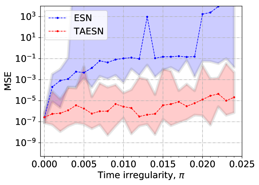
(a)

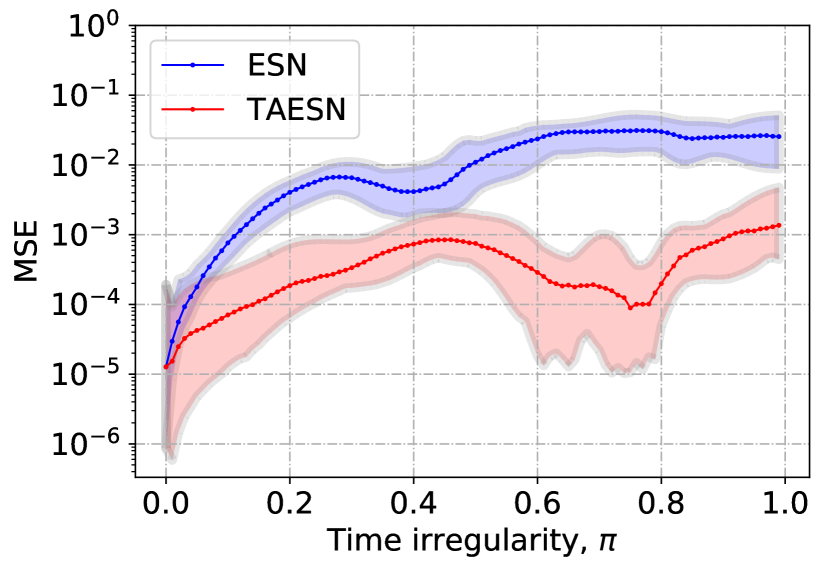
(b)

Figure 1: Comparison of ESN and TAESN error for varying time irregularity of chaotic attractor data. Dotted lines indicate median and shading indicates min/max errors over 50 runs. (a) Lorenz (b) Mackey-Glass.

We see that the performance of TAESN degrades very slowly with increasing time irregularity, which confirms the validity of our approach, while the identical regular ESN becomes unstable (confused) quite fast when encountering time-irregular data.

We also did a similar test on a more memory-demanding Mackey-Glass [17] chaotic attractor with parameters $\beta=0.2$, $n=10$, $\gamma=0.1$, and $\tau=17$. Since the attactor depends on a fixed time interval $\tau$, we had to first generate the data with a small (for this dataset) uniform $\Delta t^{\prime}=0.01$, and then produce the time-irregular data by cubic spline interpolation from this high-regular-sampling-rate data, sampling $\Delta t_{n}$ from $(1-\pi,1+\pi]$.

The results are presented in Figure 1(b). We can see that TAESN is again more robust to time-irregularity, but ESN also degrades less in this task. The systematic variations of performance depending on $\pi$ could probably be explained on how precisely the time steps hit $\tau$, as the results were repeated with the same random $\Delta t_{n}$, just scaled differently depending on $\pi$.

The GRU and LSTM RNN models performed expectedly poorly on these high-precision clean synthetic tasks because they use noisy stochastic gradient descent.

4.2 UWave gesture dataset

UWaveGestureAll [13] is a univariate time series data set consisting of gesture patterns of eight types. The dataset contains 890 training and 3 580 testing samples, where each sample consists of 900 data points. We follow the methodology used in [7] and [21] by sampling random 10% out of every sample. For evaluation, 30% of the training data was used for validation. Each trainable model was iterated for 100 epochs for 10 times with random models’ initialization. Also, each ESN variation had 500 neurons in its reservoir, while the other baselines had 100 neurons in their hidden layers. Moreover, the leaking rate and spectral radius scaling hyper-parameters for ESN variations were found using grid-search.

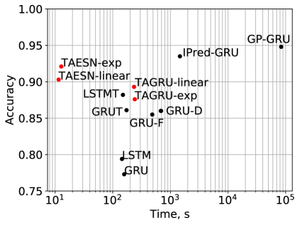
Figure 2: Time and performance comparison on UWaveGesture dataset. Proposed variations are marked in red. ESNT variation was omitted due to lower performance. Results are plotted on a logarithmic axis for clarity.

Furthermore, we compare the results reported in [21]. Concretely, we report the following baselines, that performed most notably: GRU-F, where the missing values are imputed with the last observation of the series, GRU-D [2], which adds exponential decaying in the input and the hidden state, when the variable is not observed, GRU-HD [2], where the decay is only introduced in the hidden state and not the input, GP-GRU [6], a Gaussian process, with GRU as a classifier, and IPred-GRU [21], an interpolation-prediction network with GRU as a classifier. Each of the baselines had 128 neurons in GRU classifier hidden state. The training time was scaled to match the hardware differences with [21].

From each of the training sessions, the best model based on the validation loss was chosen. Averaged results are presented in Table 1.

Table 1: Results on UWaveGestureAll dataset.

Model	Parameters	Accuracy	Training time, s	$f(\Delta t_{n})$
GRU-F* [21]	50 952	0.855	$4.840\times 10^{2}$	–
GRU-D* [2]	?	0.860	$6.810\times 10^{2}$	exp
GRU-HD* [2]	?	0.860	$6.900\times 10^{2}$	exp
GP-GRU* [6]	?	0.948	$8.365\times 10^{4}$	–
IPred-GRU* [21]	51 721	0.935	$1.463\times 10^{3}$	–
ESNT	4 016	0.567 $\pm$ 0.265	$1.101\times 10^{1}$	linear
TAESN	4 016	0.903 $\pm$ 0.011	$1.150\times 10^{1}$	linear
TAESN	4 016	0.921 $\pm$ 0.006	$1.277\times 10^{1}$	exp
LSTM	41 608	0.794 $\pm$ 0.016	$1.445\times 10^{2}$	–
LSTMT	42 008	0.882 $\pm$ 0.009	$1.500\times 10^{2}$	linear
GRU	31 408	0.773 $\pm$ 0.009	$1.579\times 10^{2}$	–
GRUT	31 708	0.861 $\pm$ 0.007	$1.733\times 10^{2}$	linear
TAGRU	31 408	0.893 $\pm$ 0.010	$2.341\times 10^{2}$	linear
TAGRU	31 408	0.876 $\pm$ 0.012	$2.410\times 10^{2}$	exp

* Results reported in [21].

From the results in Table 1 we can see that TAESNs proved to be very good in both performance and training time. We found that the regular ESN was quite sensitive to its random weight generation in this time-irregular task, which explains its poor performance and high standard deviation. TAGRU also performed significantly better than regular GRU or LSTM models and slightly better compared to versions GRUT and LSTMT that receive $\Delta t_{n}$ as inputs. The training time of TAGRU was severely impaired, because of our custom unoptimized modifications made to the standard Keras libraries.

4.3 Speleothem dataset

To evaluate RNNs on a real-world generative task, we use the readings of oxygen isotopes obtained from speleothems in the Indian cave [22] dataset. We use the first 1 800 univariate samples, of which 1 700 are used for training, 50 for validation, and the last 50 for testing. We trained conventional RNN models for 100 epochs and repeated this process for 10 times with random models’ initialization. The optimal number of neurons was found through a grid search to be 30 for the trainable RNN baselines and 50 for the ESN baselines. Grid search was also carried out to find the optimal leaking rate and spectral radius scaling for ESN variants.

Since ESNs support one-shot learning through the linear regression, we have also tested cross-validation (CV) on temporal data. Concretely, each fold consisted of 50 consecutive samples and the hyper-parameters were chosen based on the mean validation error. For testing, ESN’s readout weights were recomputed from the whole training sequence.

We have tested three variations of each RNN baseline: regular RNNs, where the model is not aware of any time-irregularities, RNNs with $\Delta t_{n}$ as an additional input, and a variation, where the RNNs received interpolated training sequence as the input. In the interpolated variation (which we refer to as “Interp.”), the whole training sequence was resampled into regular-time time series with linear interpolation before feeding it in. Then, to evaluate this model, the predicted time series with regular sampling, was again resampled with linear interpolation to match the irregular time points of the original time series, and errors where computed.

Table 2: Results on the Speleothem dataset

Model	Validation RMSE	Test RMSE	Test MAPE	$f(\Delta t_{n})$	Validation type
ESN	0.193 $\pm$ 0.005	0.185 $\pm$ 0.006	1.709 $\pm$ 0.057	–	CV
Interp. ESN	0.183 $\pm$ 0.004	0.304 $\pm$ 0.005	2.917 $\pm$ 0.051	–	CV
ESNT	0.201 $\pm$ 0.005	0.244 $\pm$ 0.001	2.340 $\pm$ 0.010	exp	CV
TAESN	0.182 $\pm$ 0.004	0.346 $\pm$ 0.014	3.333 $\pm$ 0.150	linear	CV
TAESN	0.199 $\pm$ 0.008	0.159 $\pm$ 0.002	1.478 $\pm$ 0.017	exp	CV
ESN	0.117 $\pm$ 0.009	0.425 $\pm$ 0.064	4.311 $\pm$ 0.702	–	standard
Interp. ESN	0.139 $\pm$ 0.022	0.346 $\pm$ 0.093	3.397 $\pm$ 0.998	–	standard
ESNT	0.161 $\pm$ 0.036	0.348 $\pm$ 0.044	3.377 $\pm$ 0.456	linear	standard
TAESN	0.120 $\pm$ 0.011	0.490 $\pm$ 0.021	4.952 $\pm$ 0.237	linear	standard
TAESN	0.129 $\pm$ 0.008	0.408 $\pm$ 0.026	4.125 $\pm$ 0.296	exp	standard
LSTM	0.160 $\pm$ 0.001	0.405 $\pm$ 0.009	3.999 $\pm$ 0.103	–	standard
Interp. LSTM	0.157 $\pm$ 0.002	0.383 $\pm$ 0.010	3.738 $\pm$ 0.118	–	standard
LSTMT	0.162 $\pm$ 0.001	0.403 $\pm$ 0.023	3.981 $\pm$ 0.267	linear	standard
GRU	0.169 $\pm$ 0.010	0.351 $\pm$ 0.028	3.401 $\pm$ 0.304	–	standard
Interp. GRU	0.171 $\pm$ 0.010	0.334 $\pm$ 0.022	3.206 $\pm$ 0.236	–	standard
GRUT	0.164 $\pm$ 0.003	0.366 $\pm$ 0.017	3.559 $\pm$ 0.192	linear	standard
TAGRU	0.187 $\pm$ 0.021	0.349 $\pm$ 0.053	3.389 $\pm$ 0.577	linear	standard

From the results in Table 2 it can be seen that the cross-validation proved to be especially effective for ESN-based methods, which were the only ones capable of it. This probably has something to do with (the lack of) stationarity of the time series. Evidently, TAESN with exponential time function displayed the best results among all the tested methods, including other cross-validated ones. Among the standard-validated methods the interpolated GRU model yielded the best results on the testing set, with the TAGRU, ESNT, and interpolated ESN giving similar results.

5 Discussion

Our analytically-derived models of time-adaptive RNNs (ESNs and GRUs) allow to deal with data time irregularities directly with no learning or computational overhead by letting the RNN models to “live” in the irregular time of the data and not vice versa. They tested with success in thorough numerical simulations on two synthetic and two real-world datasets.

The same time-adaptive RNN idea is in principle applicable to other fully trained RNN architectures like BPTT-trained [24] RNN or LSTM. But in this work, we preferred GRU over LSTM, because it is simpler and closer to our other method, and ESN over fully BPTT-trained classical RNN, because it is simpler and requires less training. Time-adapting other RNN models is a promising future work.

Our model also has some limitations:

• As mentioned, bigger time gaps are a problem. It is partially solved with nonlinear transformation of $\Delta t_{n}$, but in some applications filling these big gaps in data by some typo of inputation might be beneficial.

• Missing data in some inputs, but not all, is not handled by our model.

• $\Delta t_{n}$ variations are potentially invisible to the model, but can in some cases have useful information in themselves.

The time-discretization of the models could also potentially be done in a less crude way than the linear Euler approximation used here.

References

- [1] I. M. Baytas, C. Xiao, X. Zhang, F. Wang, A. K. Jain, and J. Zhou. Patient subtyping via time-aware LSTM networks. In Proceedings of the 23rd ACM SIGKDD International Conference on Knowledge Discovery and Data Mining, pages 65–74. ACM, 2017.
- [2] Z. Che, S. Purushotham, K. Cho, D. Sontag, and Y. Liu. Recurrent neural networks for multivariate time series with missing values. Scientific reports, 8(1):6085, 2018.
- [3] T. Q. Chen, Y. Rubanova, J. Bettencourt, and D. K. Duvenaud. Neural ordinary differential equations. In Advances in Neural Information Processing Systems, pages 6571–6583, 2018.
- [4] K. Cho, B. van Merrienboer, Ç. Gülçehre, F. Bougares, H. Schwenk, and Y. Bengio. Learning phrase representations using RNN encoder-decoder for statistical machine translation. CoRR, abs/1406.1078, 2014.
- [5] Y. G. Cinar, H. Mirisaee, P. Goswami, E. Gaussier, and A. Aït-Bachir. Period-aware content attention RNNs for time series forecasting with missing values. Neurocomputing, 312:177–186, 2018.
- [6] J. Futoma, S. Hariharan, and K. Heller. Learning to detect sepsis with a multitask Gaussian process RNN classifier. In Proceedings of the 34th International Conference on Machine Learning-Volume 70, pages 1174–1182. JMLR. org, 2017.
- [7] J. Futoma, S. Hariharan, M. Sendak, N. Brajer, M. Clement, A. Bedoya, C. O’Brien, and K. Heller. An improved multi-output Gaussian process RNN with real-time validation for early sepsis detection. arXiv preprint arXiv:1708.05894, 2017.
- [8] L. B. Godfrey and M. S. Gashler. Neural decomposition of time-series data for effective generalization. IEEE transactions on neural networks and learning systems, 29(7):2973–2985, 2018.
- [9] H. Jaeger. The “echo state” approach to analysing and training recurrent neural networks. Technical Report GMD Report 148, German National Research Center for Information Technology, 2001.
- [10] H. Jaeger and H. Haas. Harnessing nonlinearity: predicting chaotic systems and saving energy in wireless communication. Science, 304(5667):78–80, 2004.
- [11] H. Jaeger, M. Lukoševičius, D. Popovici, and U. Siewert. Optimization and applications of echo state networks with leaky-integrator neurons. Neural Networks, 20(3):335–352, 2007.
- [12] Z. C. Lipton, D. C. Kale, C. Elkan, and R. Wetzel. Learning to diagnose with LSTM recurrent neural networks. arXiv preprint arXiv:1511.03677, 2015.
- [13] J. Liu, L. Zhong, J. Wickramasuriya, and V. Vasudevan. uwave: Accelerometer-based personalized gesture recognition and its applications. Pervasive and Mobile Computing, 5(6):657–675, 2009.
- [14] E. N. Lorenz. Deterministic nonperiodic flow. Journal of Atmospheric Science, 20:130–141, 1963.
- [15] M. Lukoševičius. A practical guide to applying echo state networks. In G. Montavon, G. B. Orr, and K.-R. Müller, editors, Neural Networks: Tricks of the Trade, 2nd Edition, volume 7700 of LNCS, pages 659–686. Springer, 2012.
- [16] M. Lukoševičius, D. Popovici, H. Jaeger, and U. Siewert. Time warping invariant echo state networks. Technical Report No. 2, Jacobs University Bremen, May 2006.
- [17] M. C. Mackey and L. Glass. Oscillation and chaos in physiological control systems. Science, 197(4300):287–289, 1977.
- [18] M. C. Mozer, D. Kazakov, and R. V. Lindsey. Discrete event, continuous time RNNs. arXiv preprint arXiv:1710.04110, 2017.
- [19] D. Neil, M. Pfeiffer, and S.-C. Liu. Phased LSTM: Accelerating recurrent network training for long or event-based sequences. In Proceedings of the 30th International Conference on Neural Information Processing Systems, NIPS’16, pages 3889–3897, USA, 2016. Curran Associates Inc.
- [20] T. Pham, T. Tran, D. Q. Phung, and S. Venkatesh. Deepcare: A deep dynamic memory model for predictive medicine. CoRR, abs/1602.00357, 2016.
- [21] S. N. Shukla and B. Marlin. Interpolation-prediction networks for irregularly sampled time series. In International Conference on Learning Representations, 2019.
- [22] A. Sinha, G. Kathayat, H. Cheng, S. F. Breitenbach, M. Berkelhammer, M. Mudelsee, J. Biswas, and R. L. Edwards. Trends and oscillations in the indian summer monsoon rainfall over the last two millennia. Nature communications, 6:6309, 2015.
- [23] C. Tallec and Y. Ollivier. Can recurrent neural networks warp time? arXiv preprint arXiv:1804.11188, 2018.
- [24] P. J. Werbos. Backpropagation through time: what it does and how to do it. Proceedings of the IEEE, 78(10):1550–1560, 1990.
- [25] Y. Zhu, H. Li, Y. Liao, B. Wang, Z. Guan, H. Liu, and D. Cai. What to do next: Modeling user behaviors by time-LSTM. In Proceedings of the Twenty-Sixth International Joint Conference on Artificial Intelligence, IJCAI-17, pages 3602–3608, 2017.