Event Transformer

Abstract

The event camera is a bio-vision inspired camera with high dynamic range, high response speed, and low power consumption, recently attracting extensive attention for its use in vast vision tasks. Unlike the conventional cameras that output intensity frame at a fixed time interval, event camera records the pixel brightness change (a.k.a., event) asynchronously (in time) and sparsely (in space). Existing methods often aggregate events occurred in a predefined temporal duration for downstream tasks, which apparently overlook varying behaviors of fine-grained temporal events. This work proposes the Event Transformer to directly process the event sequence in its native vectorized tensor format. It cascades a Local Transformer (LXformer) for exploiting the local temporal correlation, a Sparse Conformer (SCformer) for embedding the local spatial similarity, and a Global Transformer (GXformer) for further aggregating the global information in a serial means to effectively characterize the time and space correlations from input raw events for the generation of effective spatiotemporal features used for tasks. Experimental studies have been extensively conducted in comparison to another fourteen existing algorithms upon five different datasets widely used for classification. Quantitative results report the state-of-the-arts classification accuracy and the least computational resource requirements, of the Event Transformer, making it practically attractive for event-based vision tasks.

ransformer, Sparse Convolution, Spatiotemporal Feature, Vectorized Tensor

1 Introduction

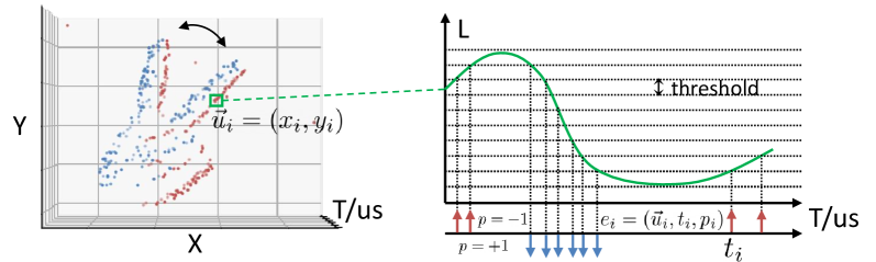
Figure 1: Event data formulation. Left: Event camera records a sequence of events asynchronously when captures a shaking gesture. Right: At each pixel position $\vec{u}_{i}=(x_{i},y_{i})$, event camera produce events $e_{i}=(u_{i},t_{i},p_{i})$ with polarity $p_{i}$ when the log brightness $L$ changes above a threshold value at timestamp $t_{i}$.

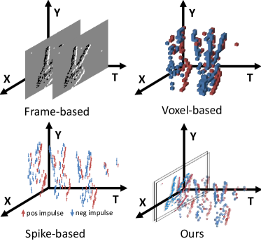
(a) Representation Forms

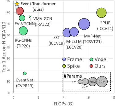
(b) Performance Gain

Figure 2: Our data representation forms and gain. (a) Different representation forms of event data. The frame-based loses the temporal information, the voxel-based lacks temporal fine-grained, the spike-based cannot be effectively optimized due to non-differentiable of impulse response function and our proposed representation treats events as a sequence of discrete tokens with image properties which can utilize the temporal information of event data and its image nature while ensuring the lossless time precision. (b) Our Event Transformer outperforms existing state of the arts while maintaining efficiency.

In contrast to a conventional camera that outputs standard intensity frame at fixed time interval, an event camera mimics the biological behavior of the retina [4] to dynamically and asynchronously capture the brightness (intensity) change of a pixel whenever it is beyond a preset threshold. As extensively reviewed in  [17], an event camera typically has a much higher response frequency (1$\mu$s vs 33ms), lower power consumption (10mW vs 300mW), and higher dynamic range (140dB vs 70dB). These advantages have led to the widespread use of event cameras in various computer vision tasks including object recognition [21, 38, 33, 27, 39, 3], detection [35], and simultaneous localization and mapping (SLAM) [6, 31].

An event camera records a sequence of events asynchronously, which can be described as

$$\textbf{E}=\left\{e_{1},\ldots,e_{n}\right\},e_{i}=(\vec{u}_{i},t_{i},p_{i}).$$ (1)

Each event $e_{i}$ is a tuple that has pixel position $\vec{u}_{i}=(x_{i},y_{i})$, polarity $p_{i}\in\{-1,1\}$ at time $t_{i}$. $p_{i}$ indicates the increase or decrease of pixel brightness as depicted in Fig. 1. To facilitate the use of event camera in downstream tasks, we first need to represent the events appropriately. Fig. 2 depicts some common representation schemes that include frame-based [34, 24, 39, 18, 11, 5, 10], voxel-based [37, 3, 9, 14, 2], and spike-based [26, 15] representations.

In this work, we propose to directly process the event sequence $\bf E$ in its native vectorized tensor format as a sequence of event words. We observe that each events $e_{i}=(\vec{u}_{i},t_{i},p_{i})$ can be viewed and represented as a word in an event sequence, akin to representation of a word in a sentence for natural language processing (NLP) applications. Different parameters for the event $(\vec{u}_{i},t_{i},p_{i})$ correspond to different words in a sentence. Note that a sentence in NLP tasks only presents word dynamics over time. In contrast, events occur sparsely over 2D space and asynchronously over time, which requires a representation that can preserve the joint spatiotemporal correlations.

This work proposes a novel Event Transformer to process the sequence of events ${\bf E}$ directly without event accumulation (e.g., averaging) to form a 2D frame, 3D voxel, or 2D spikes. To achieve this goal, we introduce a basic Event Transformer Block (ETB) that consists of three serial interconnected modules: local transformer (LXformer), sparse conformer (SCformer), and global transformer (GXformer). The LXformer module runs within a local 1D time duration to capture temporal correlations, the SCformer module takes the output from the LXformer and performs the spatial information embedding in a predefined 2D local spatial window, and the GXformer further aggregates the information of downscaled sequence from the SCformer in a global manner. We concatenate four ETBs to create the event transformer backbone to convert input event stream to a feature tensor. Our goal is to extensively exploit spatial and temporal correlations of input event sequence by local and global information processing and generate effective spatiotemporal features for downstream tasks. Since we use common operators like multilayer perceptron (MLP) and sparse convolution, our method can be easily implemented on mainstream devices. Cascaded modules in each ETB also offer computational efficiency; for instance the GXformer runs on downscaled sequence of event features that can be achieved with local computations over segments of the event sequence.

We evaluate the proposed Event Transformer on high-level event-based classification tasks. We conducted extensive experimental studies to compare our proposed method with fourteen existing models that use frame-based, voxel-based, and spike-based representation. As shown in Fig. 2b, we obtained the state-of-the-arts (SOTA) results for N-MNIST  [21] (+0.4), N-Caltech101  [33] (+1.1), CIFAR10-DVS  [27] (+1.5), N-CARS  [39] (+0.1), and ASL-DVS  [3] (+1.0) datasets respectively while reducing the amont of computational (-61%) significantly compare the previous SOTA. Our method also requires the least computational resources compared to the existing methods, which makes it a practical and useful candidate for event-based vision tasks.

The main contributions of this paper are summarized as follows.

• We propose a novel representation form vectorized tensor that takes full advantage of the image properties of the event while maintaining the fine-grained timestamps of the event.

• We propose the Event Transformer using vectorized tensor to fully extract the relationship between event and event.

• We achieve the highest accuracy on multiple datasets while also significantly reducing model computation (only 0.51G FLOPs).

2 Related Work

2.1 Event Representation Methods

Given the popularity and prevalence of deep neural network (DNN) for 2D images, it is attractive to re-use them for event cameras. A straightforward approach is to convert event sequence into a 2D image by aggregating events in a preset time duration (e.g., 33 ms) into a gray-scale frame, as shown in Fig. 2a. A number of such frame-based event representation approaches have been proposed in [34, 24, 39, 18, 11, 5, 10], but they introduces motion blur by discarding the fine time granularity in event cameras. An alternative approach is to convert events into a 3D point cloud and apply 3D DNNs for different tasks. Voxel-based representation [37, 3, 9, 14, 2] converts events into a sequence of spatially-scattered 3D voxels by aggregating events in a relatively-short time duration. Some methods [26, 15] represent events as impulses, as demonstrated in Fig 2a, which resemble spikes in human brain neurons and try to process them with the spiking neural network (SNN), Nevertheless, a spike in SNN is an impulse response function which is not differentiable. Thus, the inability of SNN to use gradient-based backpropagation and the need for specialized hardware implementation limit its applications.

2.2 Event-Based Vision

Event cameras were first used in SLAM because of their low latency and bandwidth savings compared to conventional video cameras. In SLAM, the most common vision task is the detection of calibration plates and feature points. Therefore, several methods proposed to detect corners, lines, and edges by manually designing feature extractors [7, 30, 41]. As event cameras are upgraded and popularized, they are increasingly used in tasks such as object recognition [21, 33, 27, 39, 3], detection [35], and segmentation [1]. Extracting semantic information from purely hand-designed features is extremely difficult; therefore, several methods have converted events into images to extract features with DNNs [29, 45, 34, 24, 18, 11, 5, 10]. For instance, [29] stacks a period of events into a two-channel image based on their polarity, which causes a loss of temporal information and the event data converts into a long-exposure photograph. [45] adds two channels to record the timestamp of the last event. To take full advantage of the temporal information, [39] encodes the latest events into time-surfaces, but it loses the spatial features. [18, 5] attempt to generate event frames by adaptive selection of events using learning approaches. It is worth noting that all frame-based methods require selection of a time window. A shorter window leads to insufficient accumulated data for downstream tasks, while a longer one causes motion blur and defeats the original purpose of high response rate from event cameras.

Several methods have been introduced to represent and exploit the spatio-temporal correlations in the event data by processing them as 3D points  [2, 14, 3, 9]. For instance, [2, 14] try to capture the spatio-temporal connection by 3D convolution, which is widely used in 3D medical image processing. [3, 9] use graph convolution network (GCN) to learn the relationship between events because event data are extremely sparse and 3D convolutions can be computationally intensive. The time required to build the graph structure can even exceed the time required for the recognition task itself. Furthermore, these methods pre-process data by voxelizing events, which reduces the temporal granularity of the event data. In particular, [14] processes the event data into voxels with a minimum resolution of 10ms for event super-resolution, which achieves high spatial resolution but loses the temporal resolution.

In addition to DNN and GNN, some methods [26, 15] have used spiking neural networks (SNN) for event data classification. The design of SNNs simulating human neural response and event cameras simulating retinal activation appear to be a nice combination. Nevertheless, the challenges of training SNNs and the need for special hardware prevents SNN from being used in real-life applications [40].

In summary, the current methods for processing of events face problems in combining the spatial and temporal information and preserving the fine temporal granularity. In our method, we use the raw events data as input to ensure the lossless time precision. Inspired by recent NLP literature  [12, 44, 8], we use a transformer to extract temporal features and fuse temporal features with spatial features by sparse convolutions.

2.3 Transformer

Transformer architecture was recently proposed in [42] and applied to machine translation, which contains self-attention layers without any recurrent or convolutional blocks. In recent years, transformer-based methods have achieved huge success in NLP [12, 44, 8] and vision tasks [13, 28]. Transformer-based backbones achieve better performance compared to the convolution-based backbones because of their ability to model information over long duration. Recently, [32] has used video transformer to successfully process spatio-temporal information in videos. However, previous transformers [42, 12, 44, 8, 13, 28, 32] have not been able to handle event data well The NLP transformers [42, 12, 44, 8] cannot consider the spatial information of events data, the image transformers cannot handle the temporal relationships of events, and the video transformer [32] needs to voxelize events where the sparsity of events would result in a lot of redundant computations.

3 Approach

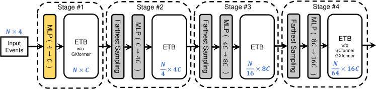
(a) Event Transformer Backbone

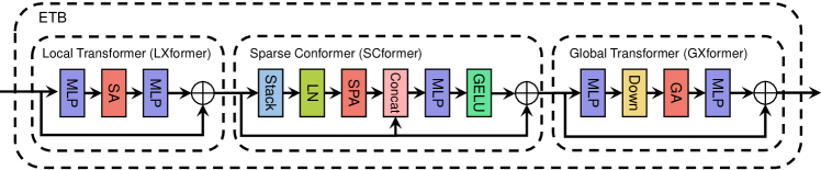
(b) Event Transformer Block

Figure 3: Event Transformer. (a) Four-stage backbone with $N\times 4$ raw events input and $\frac{N}{16}\times(16C+4)$ output. For each event, output includes the original 4-channel attributes and aggregated features. For simplicity, we only give the size of features at each stage. Linear embedding layer that uses a MLP is used at the 1st stage to map input 4-channel attributes of event to $C$-channel latent features for subsequent processing. From the 2nd to 4th stage, an event sampling layer with a farthest point downsampling and a MLP is included before the ETB step. (b) the Event Transformer Block (ETB) consist of three cascaded blocks. Self-attention (SA), sparse convolution-based attention (SPA), global attention (GA), and layer normalization (LN) are standard layers from transformers.

3.1 Backbone Architecture

Fig. 3a depicts the Event Transformer backbone that consists of four Event Transformer Blocks (ETB) to efficiently characterize the spatiotemporal correlations from input event sequence in a multistage means for output features. As shown in Fig. 3b, each ETB is formed by three serial interconnected modules: local transformer (LXformer), sparse conformer (SCformer), and global transformer (GXformer).

At the first stage, raw event sequence $\bf E$ of size $\textit{N}\times 4$ is fed into an MLP-based linear embedding layer to generate corresponding features of size $N\times C$. The original $\bf E$ is passed all the way through the Backbone used for position encoding. As a result, both events and associated features at a size of $N\times(4+C)$ are processed by the subsequent ETB. We intentionally remove the GXformer in ETB at this first stage to focus on the local information aggregation. The output of the first stage is then processed by subsequent stages.

Second to fourth stage implement the Event Sampling prior to the use of ETB. Each event sampling layer consists of a farthest point downsampling [36] step and an MLP, which reduces the number of events uniformly by a factor of 4. The feature channel size is expanded by a factor of 4, 2, and 2 for 2nd, 3rd and 4th stage respectively. These steps eventually lead to a final output of size $\frac{\textit{N}}{64}\times(16\textit{C}+4)$.

The second and third stage share the same ETB structure , while we remove the SCformer and GXformer from the ETB of the last stage. This is because the number of events are reduced significantly (i.e., from $N$ to $\frac{N}{64}$) by the aforementioned stage-wise event sampling, and a single LXformer is sufficient to capture necessary information for feature aggregation.

3.2 Local Transformer

(a) Attention $s_{im}$ between $e_{i}$ and $e_{m}$

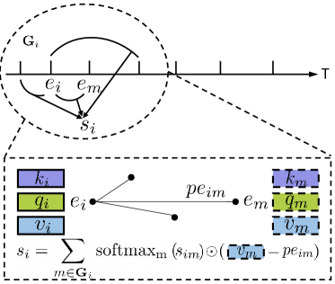
(b) Self attention $s_{i}$ of $e_{i}$

Figure 4: Self attention in LXformer. (a) The attention $s_{im}$ between $e_{i}$ and $e_{m}$ is calculated using query $q_{i}$ of $e_{i}$, key $k_{m}$ of $e_{m}$ and the distance $d_{im}$ between $e_{i}$ and $e_{j}$. (b) The self-attention $s_{i}$ is calculated using the set $G_{i}$ of events that are temporally close to event $e_{i}$.

In this section, we discuss details for the design of LXformer, SCformer, and GXformer. The input of each LXformer is an event sequence having $N$ events: $\mathbf{E}=\{e_{1},\ldots,e_{N}\}\in R^{N\times 4}$, each $e_{i}$ consists of the original 4-channel attributes. The aggregated $C$-channel features $\mathbf{F}=\left\{f_{1},\ldots,f_{N}\right\}\in R^{N\times\textit{C}}$. Other settings of $N$ and $C$ can be easily extended. We feed $\mathbf{F}$ into three different MLPs to derive the query, key, and value vectors of size $\textit{N}\times\textit{C}_{h}$, denoted as $\mathbf{Q}$, $\mathbf{K}$, and $\mathbf{V}$, respectively. To retain the position relationships between events, we define $\mathbf{D}=\{d_{11},\ldots,d_{ij},d_{NN}\}\in R^{\textit{N}\times\textit{N}\times 4}$ as the relative position and compute $\mathbf{PE}={\rm MLP}\left(\textbf{D}\right)$ to encode the relative position. As shown in Fig. 4, to exploit local correlation in 1D time dimension, we consider $M$ events that are temporally closest to $e_{i}$, and define them as $\mathbf{G}_{i}\in\mathbf{E}$. The attention between $e_{i}$ and its adjacent event $e_{m}\in\mathbf{G}_{i}$ is computed as

$$s_{im}={\rm MLP}\left(q_{i}-k_{m}+pe_{im}\right),$$ (2)

where $pe_{im}\in\mathbf{PE}$. The self attention $s_{i}$ of $e_{i}$ can be written as

$$s_{i}=\sum\limits_{m\in\mathbf{G}_{i}}{\rm softmax}_{m}\left(s_{im}\right)\odot\left(v_{m}+pe_{im}\right).$$ (3)

This finally leads to the output features $\mathbf{Y}_{\textit{local}}=\{y_{0},\ldots,y_{N}\}\in R^{N\times C}$, where

$$y_{i}=f_{i}+{\rm MLP}\left(s_{i}\right).$$ (4)

3.3 Sparse Conformer

Different from the language data that only possesses the 1D dynamics over time, events captured by the camera exhibit changes in both space and time. In addition to the local embedding using $M$ temporally-closest events in LXformer to leverage the 1D time correlations, we suggest another local embedding in 2D space to exploit 2D spatial correlations.

To incorporate spatial correlations, we first stack features of all events that occur at the same spatial position with the same polarity for averaging, and then concatenate averaged features for respective polarity levels. The sequence of events $\{(e_{i},f_{i})\}_{i=1}^{N}$ is converted to a 2D frame $\mathbf{I}\in R^{\textit{H}\times\textit{W}\times\left(2+\textit{C}\right)}$, where $H$ and $W$ are the height and width of the frame. Since there may be large differences after feature stacking, we then add a layer normalization $\mathbf{L}={\rm LN}\left(\mathbf{I}\right)$ to prevent gradient explosion.

We extract the correlation between local 2D pixels in image $\bf L$ through a sparse convolution-based attention mechanism. The attention query, key, and value vectors are obtained by three different sparse convolutions [19] as $\mathbf{Q}={\rm SPConv}_{q}(\mathbf{L})$, $\mathbf{K}={\rm SPConv}_{k}(\mathbf{L})$, $\mathbf{V}={\rm SPConv}_{v}(\mathbf{L})$. The use of sparse convolution is mainly due to the sparsely-scattered nature of events.

To reduce the computational complexity, for event $e_{i}$, we compute attention only within its surrounding window $W$ (e.g., 3$\times$3 in this study). Specifically, for event $e_{i}$ and event $e_{j}\in W$, the correlation $s_{ij}$ can be computed by their corresponding $q_{y_{i},x_{i}}=\mathbf{Q}(y_{i},x_{i}),k_{y_{j},x_{j}}=\mathbf{K}_{(}y_{i},x_{i})$ :

$$s_{ij}={\rm MLP}\left(q_{y_{i},x_{i}}-k_{y_{j},x_{j}}+pe_{ij}\right),$$ (5)

with $pe_{ij}={\rm MLP}\left(\left(y_{i},x_{i},p_{i}\right)-\left(y_{j},x_{j},p_{j}\right)\right)$. The self attention $s_{i}$ of $e_{i}$ can be written as

$$s_{i}=\sum\limits_{j\in W_{i}}{\rm softmax}_{j}\left(s_{ij}\right)\odot\left(v_{j}+pe_{ij}\right).$$ (6)

For the final output, we add an extra regression layer $\phi$ consisting of MLP and GELU activation to fuse features extracted from both 2D frame and 1D sequence into $\mathbf{Y}_{\textit{sparse}}=\{y_{0},\ldots,y_{N}\}\in R^{N\times C}$, where

$$y_{i}=f_{i}+\phi\left({\rm concat}\left(f_{i},{\rm MLP}\left(s_{i}\right)\right)\right).$$ (7)

3.4 Global Transformer

LXformer and SCformer aggregate local features in both space and time dimensions. Specifically, LXformer only allows the use of $M$ temporally-closest events, while the receptive field in SCformer is limited to the window $W_{i}$. However, for high-level vision tasks, the global relationship across all events is particularly important. If we directly enlarge the $M$ events in LXformer to all events, the computational complexity will increase from N to $\textit{N}^{2}$, which can become infeasible for large $N$.

To effectively process and embed global information without adding too much computation, we proposed to down-sample the number of events from N to M to obtain global $\mathbf{\hat{Q}},\mathbf{\hat{V}}$ and then compute attention map with local $\mathbf{K}$ from the original resolution. More specifically, we use the farthest point down-sampling with down-sample rate r to select the most representative events $\mathbf{\hat{E}}$. For each $e_{j}\in\mathbf{\hat{E}}$, its corresponding feature $\hat{f}_{j}\in\mathbf{\hat{F}}$ is calculated as

$$\begin{split}\hat{f}_{j}=\max_{k}\left({\rm MLP}\left({\rm concat}\left(e_{k},f_{k}\right)\right)\right),\end{split}$$ (8)

where $e_{k}\in\mathbf{G}_{j}$ and $\mathbf{G}_{j}$ is the $\lfloor\frac{1}{\textit{r}}\rfloor$ nearest events of $e_{j}$. Afterwards, MLP is used to map downsampled features $\mathbf{\hat{F}}\in R^{\textit{M}\times\textit{C}}$ to global query $\mathbf{\hat{Q}}\in R^{\textit{M}\times C_{h}}$ and global value $\mathbf{\hat{V}}\in R^{\textit{M}\times\textit{C}_{h}}$, respectively. To enable global influence of the local features, local key $\mathbf{K}={\rm MLP}(F)\in R^{N\times C_{h}}$ is used to extract local information.

The output of global attention layer $s_{i}$ can be written as

$$s_{i}=\sum\limits_{j\in\mathbf{\hat{E}}}{\rm softmax}_{j}\left(s_{ij}\right)\odot\left(\hat{v}_{j}+pe_{ij}\right),$$ (9)

where $s_{ij}=\textit{MLP}\left(k_{i}-\hat{q}_{j}+pe_{ij}\right)$ and $pe_{ij}$ is calculated the same as the position encoding in LXformer. Similar to the LXformer, we have the final output $\mathbf{Y}_{\textit{global}}=\{y_{0},\ldots,y_{N}\}\in R^{N\times C}$ with

$$y_{i}=f_{i}+{\rm MLP}\left(s_{i}\right).$$ (10)

4 Experiment

In this section, we present our experiments to evaluate the classification performance of our proposed event transformer and existing methods.

4.1 Event-Based Classification

Datasets and metrics. We test our model on five event-based classification datasets: N-MNIST [21], N-Caltech101 [33], CIFAR10-DVS [27], N-Cars [39] and ASL-DVS [3]. As shown in Table. 1, these datasets vary significantly in terms of captured camera, source of events, average duration of event stream, and dataset size. N-MNIST, N-Caltech101 and CIFAR10-DVS were shot with a laboratory version of event camera (Asynchronous Time-based Image Sensor Lab Sensor). The data capture equipment consists of an e-link screen, a movable tripod head, and an event camera. Images from the existing MNIST [25], Caltech101 [16] and CIFAR-10 [22] are displayed on the monitor and the tripod head for the event camera is moved to generate events. Since the e-link screen does not refresh while the content remains unchanged, noisy events due to screen refresh are avoided. These events arise due to camera shake, which is different from events generated by motion in the real world. N-Cars used the event camera (Prophesee Gen1) to record 24,029 sequences of 100ms on the city roads, and split them into cars and background. ASL-DVS is a 24-class dataset of handshape recordings under realistic conditions using DAVIS240c. Compared to the previous datasets, ASL-DVS has ten times more event sequences. We train our model on the training set of each dataset separately and evaluate the Top-1 classification accuracy on the test set. For datasets (N-Caltech101, CIFAR10-DVS and ASL-DVS) without official division between training and test sets, we follow the setup introduced in  [3, 9, 43] and randomly sample 80% of the data for training and the remaining 20% for testing.

Table 1: List of Event-based Classifiaction Datasets

Dataset	Camera	Source$\dagger$	Avg$\ddagger$	Data Size	Classes
N-MNIST [21]	ATIS lab sensor	shake cam	360ms	60000	10
N-Caltech101 [33]	ATIS lab sensor	shake cam	300ms	8246	101
CIFAR10-DVS [27]	ATIS lab sensor	shake cam	1280ms	10000	10
N-Cars [39]	Prophesee Gen1	real move	100ms	24029	2
ASL-DVS [3]	DAVIS240c	real move	100ms	100800	24

• Source of generating events.

• Average duration of event stream.

Implementation details. For the classification task, we average the stage 4 output features of all events and feed them into a classification head consisting of MLPs and ReLU to get the final output category. The number of channels $C$ for stage 1 is set to 32. The interactive events $M$ in LXformer is set to 16. While number of the SCformer kernels is set to [64, 128, 256] for stage 1, 2, and 3, respectively. The size of window $W$ in SCformer is set to 3. And the farthest down-sampleing rate $r$ in GXformer is set to $32$. At training time, 1024 events are randomly sampled from the training set as input, and all events are input during inference. We train our model from scratch for 200 epochs by optimizing the cross-entropy loss using the SGD optimizer with momentum 0.9 and the batch size of 64. The learning rate starts from 0.01 and decays to 0.001 and 0.0001 at 150 and 180 epochs, respectively. The whole training process takes only a few hours (e.g., only three hours for N-Caltech101).

Table 2: Accuracy of Event-based Classification Using Various Datasets. N-M refers to N-MNIST, N-Cal to N-Caltech101, CIF10 to CIFAR10-DVS, N-C to N-Cars, and ASL to ASL-DVS.

Method	Type	N-M [21]	N-Cal [33]	CIF10 [27]	N-C [39]	ASL [3]
H-First [34]	frame	0.712	0.054	0.077	0.561	-
HOTS [24]	frame	0.808	0.210	0.271	0.624	-
HATS [39]	frame	0.991	0.642	0.524	0.902	-
EST [18]	frame	0.990	0.753	0.634	0.919	0.979
AMAE [11]	frame	0.983	0.694	0.620	0.936	0.984
M-LSTM [5]	frame	0.986	0.738	0.631	0.927	0.980
MVF-Net [10]	frame	0.981	0.687	0.599	0.927	0.971
ResNet-50 [20]	frame	0.984	0.637	0.558	0.903	0.886
EventNet [37]	voxel	0.752	0.425	0.171	0.750	0.833
RG-CNNs [3]	voxel	0.990	0.657	0.540	0.914	0.901
EV-VGCNN [9]	voxel	0.994	0.748	0.651	0.953	0.983
VMV-GCN [43]	voxel	0.995	0.778	0.663	0.932	0.989
Gabor-SNN [26]	spike	0.837	0.196	0.245	0.789	-
PLIF [15]	spike	0.996	-	0.697	-	-
Ours	tensor	0.999	0.789	0.712	0.954	0.999

Experimental results. We compare Top-1 classification accuracy obtained from our model with frame-based methods (H-First [34], HOTS [24], HATS [39], EST [18], AMAE [11], M-LSTM [5], MVF-Net [10] and ResNet-50 [20]), voxel-based methods (EventNet [37], RG-CNNs [3], EV-VGCNN [9] and VMV-GCN [43]) and spike-based methods (Gabor-SNN [26] and PLIF [15]). The models in EST [18], M-LSTM [5] and MVF-Net [10] were pretrained using ImageNet [23]; for a fair comparison, we used the results from  [43] that trains networks from scratch. For PLIF [15], the original paper divides the dataset into 9:1 for training and testing; therefore, we report the results by retraining their model with 80/20% train/test split using their official code. As shown in Table 2, our model achieves state-of-the-art results on all of the classification datasets which illustrates the effectiveness of our model and representation form.

4.2 Computational Requirements Analysis

We compare the number of parameters (Parameters), the floating point operations (FLOPs), and the final accuracy of different methods on the CIFAR10-DVS dataset in Table 3. We do not list the spike-based methods because they require special hardware devices for their inference. As shown in Table 3, we get the best performance using the least amount of computation (only 0.51G FLOPs). Our method requires a larger number of parameters compared to voxel-based methods because of a large number MLP modules. Thus, our proposed even transformer is suitable for low-power devices in conjunction with event camera, where the computational cost is the primary concern.

Table 3: Model Complexity of Different Methods

Method	Type	Parameters	FLOPs	Top-1 Accuracy
EST [18]	frame	21.38M	4.28G	52.4
M-LSTM [5]	frame	21.43M	4.82G	63.1
MVF-Net [10]	frame	33.62M	5.62G	59.9
ResNet-50 [20]	frame	25.61M	3.87G	55.8
EventNet [37]	voxel	2.81M	0.91G	17.1
RG-CNNs [3]	voxel	19.46M	0.79G	54.0
EV-VGCNN [9]	voxel	0.84M	0.70G	65.1
VMV-GCN [43]	voxel	0.86M	1.30G	66.3
Ours	tensor	15.87M	0.51G	71.2

4.3 Ablation Study

We conduct a number of experiments with various setting of our model as an ablation study on CIFAR10-DVS. First we analyze the efficiency of our LXformer, SCformer, and GXformer. Then we analyze the fusion process of LXformer and SCformer. Finally, we analyze the effect of the number of interactive events in LXformer, SCformer and GXformer.

Network structure. We demonstrate that each part of our network is essential through several sets of experiments. Table 4 shows different components of the network structure, where L, S, and G represent LXformer, SCformer and GXformer, respectively. For the comparision of Local and Local+Sparse, we found that the addition of SCformer significantly improved the model’s representation ability (+1.8). Local+Sparse+Global shows that the addition of GXformer can further aggregate global information and improve performance (+1.2). We also experimented with the placement of LXformer, SCformer, and GXformer (Global+Local+Sparse and Local+Sparse+Global), and the experimental results showed that premature aggregation of spatial and global information is not conducive to the model performance (-1.4 and -1.6). We believe that this is due to the fact that temporal relationship is the most fundamental property for event data.

Table 4: Ablation Study of Network Structure

Type	Structure	Top-1 Accuracy
Local	[L, L, L, L]	68.2
Local+Sparse	[LS, LS, LS, L]	70.0
Sparse+Local+Global	[SL, SLG, SLG, L]	69.8
Global+Local+Sparse	[LS, GLS, GLS, L]	69.6
Local+Sparse+Global	[LS, LSG, LSG, L]	71.2

Fusion of LXformer and SCformer. The LXformer extracts temporal features, while the SCformer extracts spatial features. We conducted a series of experiments to find the best way to fuse the two sets of features. Table 5 presents results when we try to fuse the features in three ways: Concatenate, Parallel, and Serial. In Concatenate setting, we try to connect two completely different features together by concatenating them, and then adding them to the input features after reducing their dimension using an MLP. As shown in the Table 5, this will have an adverse impact on the model performance (-9.2). We believe this is because of the lack of residual connection between input features and output features both in LXformer and SCformer, which is important for transormers. Then we compared the performance of connecting the two features in parallel and series. The experimental results show that the temporal information aggregated by LXformer can help SCformer to extract the spatial information when using serial fusion (+1.2). Therefore we chose to place the SCformer module after the LXformer module in our proposed model.

Table 5: Ablation Study of Fusion of LXformer and SCformer

Type	Combination$\dagger$	Top-1 Accuracy
Concatenate	Y = X + MLP(Concat(L(X)+S(X)))	62.0
Parallel	Y = X + L(X)+S(X)	70.0
Serial	Y = X + S(X+L(X))	71.2

• Symbol definition: X is the input features, Y is the output, L is the LXformer and S is the SCformer.

Number of closest events in LXformer. In LXformer, we interact each event with $M$ events that occur adjacent to it in the temporal sequence, and here we experiment with the number of closeest events. Table 6 shows that when the number of closest events is small ($M=4$ or $M=8$), LXformer cannot extract enough content information (the performance drops -5.4 and -1.2, respectively). When the number is very large ($M=32$ or $M=64$), it introduces too many noisy events and causes a loss of attention (the performance drops -0.3 and -1.6, respectively).

Table 6: Ablation Study of Closest Events in LXformer

$M$ Closest Events in LXformer	4	8	16	32	64
Top-1 Accuracy	65.8	69.0	71.2	70.9	69.6

Size of interactive window in SCformer. In SCformer, we compute self attention for each event in the frame plane for a window size of $W$. Therefore, we experimented with the size of the window $W$. The experimental results shown in Table 7 illustrate that if the window size is $1\times 1$, the self attention degenerates to a general conv. The best results are achieved when the window size is $3\times 3$. And when the window size is further increased, it does not bring better gain.

Table 7: Ablation Study of Window Size in SCformer

Size of $W$ in SCformer	$1\times 1$	$3\times 3$	$5\times 5$	$7\times 7$	$9\times 9$
Top-1 Accuracy	69.9	71.2	71.1	71.0	70.6

Down-sample rate in GXformer. Finally, we evaluated the impact of down-sampling rate $r$ in GXformer on the model performance. As shown in Table 8, when the down-sampling rate $r$ is 1, which means no down-sampling, GXformer degenerates to LXformer. The experimental results show that when the $r$ is small (1 and 8), the global information extracted is not comprehensive (-1.4 and -0.9). And when the $r$ is too larger (64 and 128), it leads to excessive information loss (-0.6 and -1.1). Therefore we finally choose a downsampling rate of 32.

Table 8: Ablation Study of Down-sample Rate in GXformer

Down-sample rate r in GXformer	1	8	32	64	128
Top-1 Accuracy	69.8	70.3	71.2	70.6	70.1

5 Conclusion

Existing methods for processing event camera data lose the fine temporal granularity of events. In this paper, we consider event data as a sequence of event words, and process them sequentially while capturing and exploiting the spatial and temporal correlations in the data. Inspired by the transformer-based methods, which have had great success in natural language processing, we propose a novel Event Transformer that combines the time-domain sequence property of event data with the space-domain nature of the images. Our experiments demonstrate that our proposed model achieves the state-of-the-art results on classification. We hope our work can provides a new way of processing event data for a variety of vision tasks.

References

- [1] Alonso, I., Murillo, A.C.: Ev-segnet: Semantic segmentation for event-based cameras. In: Proceedings of the IEEE/CVF Conference on Computer Vision and Pattern Recognition Workshops. pp. 0–0 (2019)
- [2] Baldwin, R., Almatrafi, M., Asari, V., Hirakawa, K.: Event probability mask (epm) and event denoising convolutional neural network (edncnn) for neuromorphic cameras. In: Proceedings of the IEEE/CVF Conference on Computer Vision and Pattern Recognition. pp. 1701–1710 (2020)
- [3] Bi, Y., Chadha, A., Abbas, A., Bourtsoulatze, E., Andreopoulos, Y.: Graph-based spatio-temporal feature learning for neuromorphic vision sensing. IEEE Transactions on Image Processing 29, 9084–9098 (2020)
- [4] Brandli, C., Berner, R., Yang, M., Liu, S.C., Delbruck, T.: A 240 180 130 db 3 s latency global shutter spatiotemporal vision sensor. IEEE Journal of Solid-State Circuits 49(10), 2333–2341 (2014)
- [5] Cannici, M., Ciccone, M., Romanoni, A., Matteucci, M.: A differentiable recurrent surface for asynchronous event-based data. In: European Conference on Computer Vision. pp. 136–152. Springer (2020)
- [6] Censi, A., Strubel, J., Brandli, C., Delbruck, T., Scaramuzza, D.: Low-latency localization by active led markers tracking using a dynamic vision sensor. In: 2013 IEEE/RSJ International Conference on Intelligent Robots and Systems. pp. 891–898. IEEE (2013)
- [7] Clady, X., Ieng, S.H., Benosman, R.: Asynchronous event-based corner detection and matching. Neural Networks 66, 91–106 (2015)
- [8] Dai, Z., Yang, Z., Yang, Y., Carbonell, J., Le, Q.V., Salakhutdinov, R.: Transformer-xl: Attentive language models beyond a fixed-length context. arXiv preprint arXiv:1901.02860 (2019)
- [9] Deng, Y., Chen, H., Chen, H., Li, Y.: Ev-vgcnn: A voxel graph cnn for event-based object classification. arXiv preprint arXiv:2106.00216 (2021)
- [10] Deng, Y., Chen, H., Li, Y.: Mvf-net: A multi-view fusion network for event-based object classification. IEEE Transactions on Circuits and Systems for Video Technology (2021)
- [11] Deng, Y., Li, Y., Chen, H.: Amae: Adaptive motion-agnostic encoder for event-based object classification. IEEE Robotics and Automation Letters 5(3), 4596–4603 (2020)
- [12] Devlin, J., Chang, M.W., Lee, K., Toutanova, K.: Bert: Pre-training of deep bidirectional transformers for language understanding. arXiv preprint arXiv:1810.04805 (2018)
- [13] Dosovitskiy, A., Beyer, L., Kolesnikov, A., Weissenborn, D., Zhai, X., Unterthiner, T., Dehghani, M., Minderer, M., Heigold, G., Gelly, S., et al.: An image is worth 16x16 words: Transformers for image recognition at scale. arXiv preprint arXiv:2010.11929 (2020)
- [14] Duan, P., Wang, Z.W., Zhou, X., Ma, Y., Shi, B.: Eventzoom: Learning to denoise and super resolve neuromorphic events. In: Proceedings of the IEEE/CVF Conference on Computer Vision and Pattern Recognition. pp. 12824–12833 (2021)
- [15] Fang, W., Yu, Z., Chen, Y., Masquelier, T., Huang, T., Tian, Y.: Incorporating learnable membrane time constant to enhance learning of spiking neural networks. In: Proceedings of the IEEE/CVF International Conference on Computer Vision. pp. 2661–2671 (2021)
- [16] Fei-Fei, L., Fergus, R., Perona, P.: Learning generative visual models from few training examples: An incremental bayesian approach tested on 101 object categories. In: 2004 conference on computer vision and pattern recognition workshop. pp. 178–178. IEEE (2004)
- [17] Gallego, G., Delbruck, T., Orchard, G., Bartolozzi, C., Taba, B., Censi, A., Leutenegger, S., Davison, A., Conradt, J., Daniilidis, K., et al.: Event-based vision: A survey. arXiv preprint arXiv:1904.08405 (2019)
- [18] Gehrig, D., Loquercio, A., Derpanis, K.G., Scaramuzza, D.: End-to-end learning of representations for asynchronous event-based data. In: Proceedings of the IEEE/CVF International Conference on Computer Vision. pp. 5633–5643 (2019)
- [19] Graham, B., van der Maaten, L.: Submanifold sparse convolutional networks. arXiv preprint arXiv:1706.01307 (2017)
- [20] He, K., Zhang, X., Ren, S., Sun, J.: Deep residual learning for image recognition. In: Proceedings of the IEEE conference on computer vision and pattern recognition. pp. 770–778 (2016)
- [21] Iyer, L.R., Chua, Y., Li, H.: Is neuromorphic mnist neuromorphic? analyzing the discriminative power of neuromorphic datasets in the time domain. Frontiers in neuroscience 15, 297 (2021)
- [22] Krizhevsky, A., Hinton, G., et al.: Learning multiple layers of features from tiny images (2009)
- [23] Krizhevsky, A., Sutskever, I., Hinton, G.E.: Imagenet classification with deep convolutional neural networks. Advances in neural information processing systems 25 (2012)
- [24] Lagorce, X., Orchard, G., Galluppi, F., Shi, B.E., Benosman, R.B.: Hots: a hierarchy of event-based time-surfaces for pattern recognition. IEEE transactions on pattern analysis and machine intelligence 39(7), 1346–1359 (2016)
- [25] LeCun, Y.: Mnist handwritten digit database, yann lecun, corinna cortes and chris burges. URL: http://yann. lecun. com/exdb/mnist [Online (2013)
- [26] Lee, J.H., Delbruck, T., Pfeiffer, M.: Training deep spiking neural networks using backpropagation. Frontiers in neuroscience 10, 508 (2016)
- [27] Li, H., Liu, H., Ji, X., Li, G., Shi, L.: Cifar10-dvs: an event-stream dataset for object classification. Frontiers in neuroscience 11, 309 (2017)
- [28] Liu, Z., Lin, Y., Cao, Y., Hu, H., Wei, Y., Zhang, Z., Lin, S., Guo, B.: Swin transformer: Hierarchical vision transformer using shifted windows. arXiv preprint arXiv:2103.14030 (2021)
- [29] Maqueda, A.I., Loquercio, A., Gallego, G., García, N., Scaramuzza, D.: Event-based vision meets deep learning on steering prediction for self-driving cars. In: Proceedings of the IEEE Conference on Computer Vision and Pattern Recognition. pp. 5419–5427 (2018)
- [30] Mueggler, E., Bartolozzi, C., Scaramuzza, D.: Fast event-based corner detection (2017)
- [31] Mueggler, E., Huber, B., Scaramuzza, D.: Event-based, 6-dof pose tracking for high-speed maneuvers. In: 2014 IEEE/RSJ International Conference on Intelligent Robots and Systems. pp. 2761–2768. IEEE (2014)
- [32] Neimark, D., Bar, O., Zohar, M., Asselmann, D.: Video transformer network. In: Proceedings of the IEEE/CVF International Conference on Computer Vision. pp. 3163–3172 (2021)
- [33] Orchard, G., Jayawant, A., Cohen, G.K., Thakor, N.: Converting static image datasets to spiking neuromorphic datasets using saccades. Frontiers in neuroscience 9, 437 (2015)
- [34] Orchard, G., Meyer, C., Etienne-Cummings, R., Posch, C., Thakor, N., Benosman, R.: Hfirst: A temporal approach to object recognition. IEEE transactions on pattern analysis and machine intelligence 37(10), 2028–2040 (2015)
- [35] Perot, E., de Tournemire, P., Nitti, D., Masci, J., Sironi, A.: Learning to detect objects with a 1 megapixel event camera. arXiv preprint arXiv:2009.13436 (2020)
- [36] Qi, C.R., Yi, L., Su, H., Guibas, L.J.: Pointnet++: Deep hierarchical feature learning on point sets in a metric space. arXiv preprint arXiv:1706.02413 (2017)
- [37] Sekikawa, Y., Hara, K., Saito, H.: Eventnet: Asynchronous recursive event processing. In: Proceedings of the IEEE/CVF Conference on Computer Vision and Pattern Recognition. pp. 3887–3896 (2019)
- [38] Serrano-Gotarredona, T., Linares-Barranco, B.: Poker-dvs and mnist-dvs. their history, how they were made, and other details. Frontiers in neuroscience 9, 481 (2015)
- [39] Sironi, A., Brambilla, M., Bourdis, N., Lagorce, X., Benosman, R.: Hats: Histograms of averaged time surfaces for robust event-based object classification. In: Proceedings of the IEEE Conference on Computer Vision and Pattern Recognition. pp. 1731–1740 (2018)
- [40] Tavanaei, A., Ghodrati, M., Kheradpisheh, S.R., Masquelier, T., Maida, A.: Deep learning in spiking neural networks. Neural networks 111, 47–63 (2019)
- [41] Vasco, V., Glover, A., Bartolozzi, C.: Fast event-based harris corner detection exploiting the advantages of event-driven cameras. In: 2016 IEEE/RSJ International Conference on Intelligent Robots and Systems (IROS). pp. 4144–4149. IEEE (2016)
- [42] Vaswani, A., Shazeer, N., Parmar, N., Uszkoreit, J., Jones, L., Gomez, A.N., Kaiser, Ł., Polosukhin, I.: Attention is all you need. In: Advances in neural information processing systems. pp. 5998–6008 (2017)
- [43] Xie, B., Deng, Y., Shao, Z., Liu, H., Li, Y.F.: Vmv-gcn: Volumetric multi-view based graph cnn for event stream classification. IEEE Robotics and Automation Letters (2022)
- [44] Yang, Z., Dai, Z., Yang, Y., Carbonell, J., Salakhutdinov, R.R., Le, Q.V.: Xlnet: Generalized autoregressive pretraining for language understanding. Advances in neural information processing systems 32 (2019)
- [45] Zhu, A.Z., Yuan, L., Chaney, K., Daniilidis, K.: Ev-flownet: Self-supervised optical flow estimation for event-based cameras. arXiv preprint arXiv:1802.06898 (2018)