An approach to improving
sound-based vehicle speed estimation

Abstract

We consider improving the performance of a recently proposed sound-based vehicle speed estimation method. In the original method, an intermediate feature, referred to as the modified attenuation (MA), has been proposed for both vehicle detection and speed estimation. The MA feature maximizes at the instant of the vehicle’s closest point of approach, which represents a training label extracted from video recording of the vehicle’s pass by. In this paper, we show that the original labeling approach is suboptimal and propose a method for label correction. The method is tested on the VS10 dataset, which contains $304$ audio-video recordings of ten different vehicles. The results show that the proposed label correction method reduces average speed estimation error from $7.39$ km/h to $6.92$ km/h. If the speed is discretized into $10$ km/h classes, the accuracy of correct class prediction is improved from $53.2\%$ to $53.8\%$, whereas when tolerance of one class offset is allowed, accuracy is improved from $93.4\%$ to $94.3\%$.

I Introduction

Traffic analysis and planning represent indispensable parts of an intelligent transportation system. Large volumes of traffic data enable significant improvements in the performance of transportation, traffic safety and automatic traffic monitoring (TM) [1]. The TM data are used for valuable information extraction [2], which may include vehicle count [3, 4], shape [5, 6], speed [7, 8], acceleration [9], type [10, 11], plate number [12] and may be used to predict road accidents [13, 14].

Diverse sensing technologies are utilized in modern TM systems. Some of them involve induction loops, piezoelectric and magnetic sensors, ground and aerial cameras, acoustic sensors, Doppler radar and LIDAR [1]. A study conducted in [15] describes recent advances in computer vision applied in multi-camera vehicle tracking and identification, as well as traffic anomaly detection. TM based solely on vision data is often not sufficient due to sensitivity of image sensors to adverse weather conditions, lighting changes, vehicle headlights and shadows [1, 16, 14, 17].

Advantages of the acoustic-based TM over the other technologies include low price, low energy consumption and low storage space required. Acoustic sensors are easier to install and maintain and are not affected by visual occlusions and lighting variations. They are also less disturbing to drivers’ behavior and have fewer privacy issues [1], [18]. Current acoustic TM methods, described in [7], can be divided into single-microphone [19, 20, 21, 22, 23, 24, 25, 26] and microphone-array approaches [27, 28, 29].

One of important concerns in machine learning and deep learning applications for acoustic vehicle detection and speed estimation is the lack of high-quantity and high-quality annotated data [21, 22, 25, 24, 29, 26]. Furthermore, deep neural networks tend to overfit to corrupted labels, which results in poor generalization on the test dataset [30]. This is why robust training, in the presence of noisy labels, is an important task in supervised learning applications [31].

In this paper, we consider improving the accuracy of single-sensor acoustic vehicle detection and speed estimation, proposed in [7]. The original method introduced an analytical speed-dependent feature, referred to as the modified attenuation (MA), which maximizes at the instant of the vehicle’s closest point of approach (CPA). The CPA instant is represented by a training label manually extracted from video recording of the vehicle’s pass by. This labeling procedure is not optimal due to inconsistent camera view angles at installation sites. Time offset, caused by suboptimal labeling approach, is referred to as the labeling noise. This paper addresses label correction aimed to improve the accuracy of vehicle speed estimation. To that end, we propose to shift the ground-truth CPA instants by amount obtained from the test phase of the MA prediction. This approach yields notable speed estimation accuracy improvement.

We first overview the original speed estimation approach in Section II and then propose label correction method in Section III. Experimental results are given in Section IV and conclusions are drawn in Section V.

II Speed Estimation

II-A Data

Audio recordings dataset from [7], referred to as VS10, is used to train and test the speed estimation method. Recordings were captured with a GoPro Hero5 Session camera and divided into $304$ single-vehicle and $71$ environmental-noise audio-video files. Ten different vehicles are included, as reported in Table I in [7]. Vehicles’ speeds range from $30$ km/h to $105$ km/h. Audio data are extracted from video recordings. Audio files are clipped to $10$ seconds with $44100$ Hz sampling rate and saved in WAV format with $32$-bit float PCM. Dataset labels contain the vehicle’s speed and its pass-by time (CPA instant). The pass-by instant is obtained manually by identifying the time frame of a vehicle starting to exit the camera view.

II-B Acoustic features

In this paper, we use modified attenuation, originally proposed in [7] for both vehicle detection and speed estimation. The MA feature represents a modification of the amplitude attenuation factor of the sound signal [20].

The MA feature is defined as follows:

$$\eta(t)=\frac{\alpha}{\beta v^{2}(t_{\text{CPA}}-t)^{2}+d_{\text{CPA}}^{2}}$$ (1)

where $v$ denotes the speed of vehicle, $t$ is time, $t_{\text{CPA}}$ is the CPA time instant, and $d_{\text{CPA}}$ denotes the vehicle distance at CPA. Vertical and horizontal extents of $\eta(t)$ are adjusted by $\alpha$ and $\beta$, respectively. Appropriate settings of $\alpha$ and $\beta$ are outlined in Section II-D.

MA is predicted in a supervised fashion from the log-mel spectrogram (LMS) of input audio. LMS represents a very popular feature in acoustic classification applications [32] and it proved very reliable in vehicle detection and speed estimation [3, 4, 8].

II-C Method

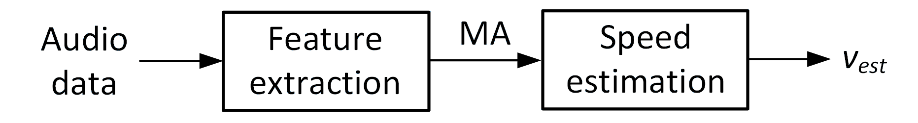
Figure 1: Block diagram of the speed estimation method.

The vehicle speed estimation method is introduced in [7] and outlined in Fig. 1. In the first step, input audio signal is transformed to its short-time power spectrum representation, namely LMS. LMS remaps original audio frequencies to their logarithmic mel scale. Next, the MA feature regression is performed using a fully-connected deep neural network (DNN). One example of MA prediction is presented in Fig. 2. The second step comprises speed estimation from the predicted MA. The vehicle’s pass-by time, denoted as $t_{\text{CPA}}$ and estimated by maximizing the MA profile, is used to detect the vehicle and select an appropriate interval of predicted MA samples for speed estimation. Finally, the speed is estimated using the selected MA samples. As in [7], $\varepsilon$-support vector regression ($\varepsilon$-SVR) [33] is used in speed estimation due to relatively small size of the dataset.

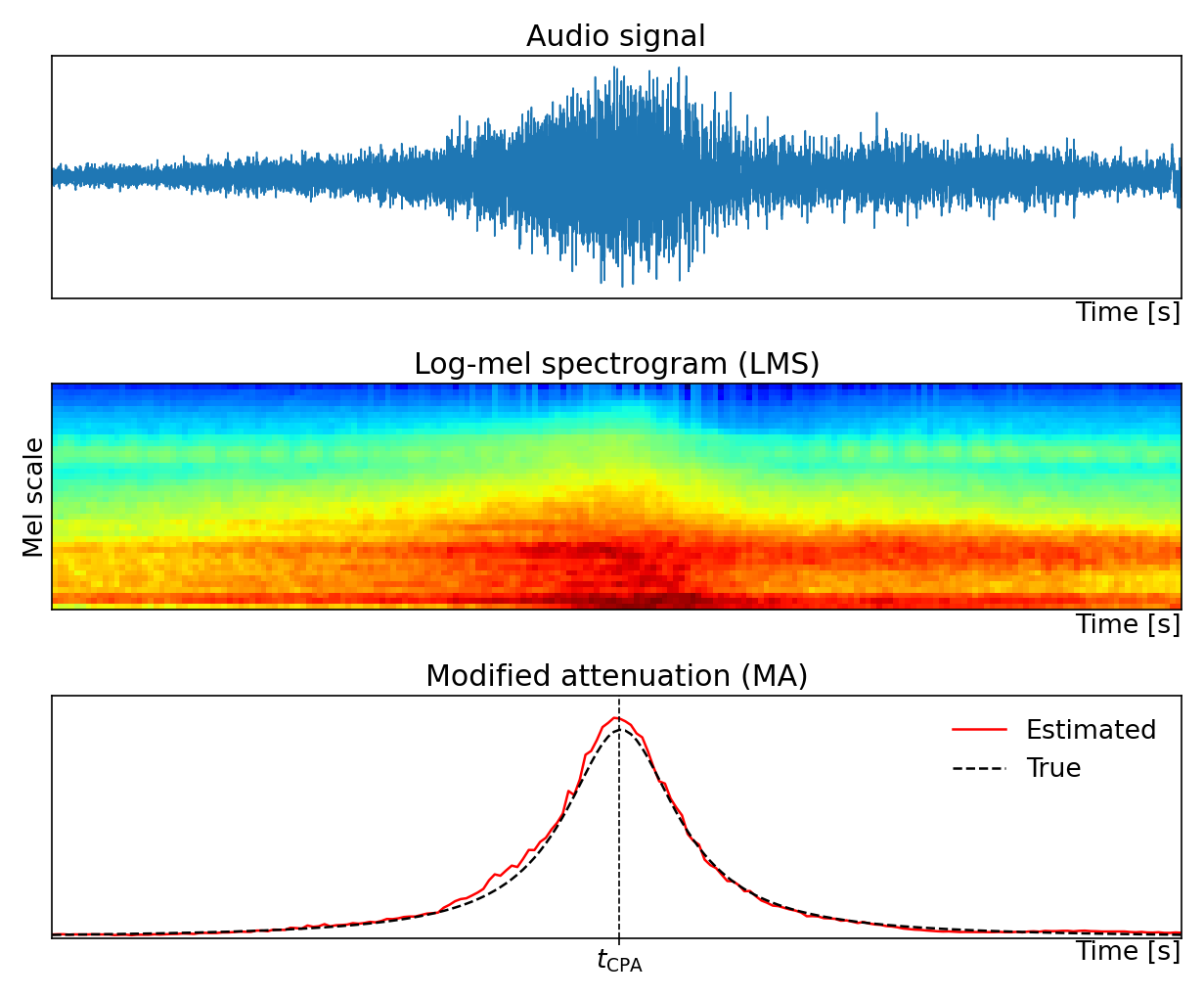
Figure 2: Top: Original audio signal of vehicle’s pass-by (speed $80$ km/h). Middle: Log-mel spectrogram of audio signal. Bottom: True and estimated MA features.

II-D Implementation details

II-D1 Features for MA regression

Original audio signals are clipped to $10$ seconds with the sampling rate of $44100$ Hz. LMS of audio is calculated using the short-time Fourier transform (STFT). STFT is calculated with $4096$-sample Hamming window and $1105$-sample hop rate, which results in $400$ time frames of STFT [34]. For each time frame, $N_{mel}=40$ mel coefficients are computed, within the frequency interval of $[0,16\text{ kHz}]$.

The MA feature (1) is calculated with $\alpha=v$, $\beta=0.05$ and $d_{\text{CPA}}=1.5$ m. The MA value, at instant $t$, is estimated using a window of LMS features comprising $Q=25$ time frames (stride of $3$), centered at $t$. This setting yields $M=Q\times N_{mel}=1000$ LMS input features. Fully-connected DNN consists of $1000$–$200$–$50$–$10$–$1$ neurons per layer. DNN is implemented using mean squared error loss, ReLU activation (linear activation in the last layer), $L2$ kernel regularization with factor $10^{-3}$ and $200$ training epochs.

II-D2 Speed estimation

Optimal $\varepsilon$-SVR parameters, namely $C=10$ and $\varepsilon=0.1$, are obtained by a grid search. A vector of $73$ adjacent MA coefficients, centered at $t_{\text{CPA}}$, represents input features of the $\varepsilon$-SVR block.

The speed estimation model is evaluated with $10$-fold cross-validation. Nine folds (vehicles) are used in training and validation, while the remaining fold is put aside for testing. Training and validation datasets are split in a $80\%$-$20\%$ fashion, as described in Section II-B in [7]. The training procedure is repeated $20$ times and the results are averaged.

III Noisy Labels Correction

Precise prediction of $t_{\text{CPA}}$ is of pivotal importance for accurate speed estimation. As mentioned in Section II-C, $t_{\text{CPA}}$ is estimated by maximizing the predicted MA feature. The vehicle’s speed is then estimated from a window of MA samples centered at $t_{\text{CPA}}$ (see Section II-D2).

The VS10 recordings, described in Section II-A, were captured with a camera installed at the side of a local road close to Podgorica, Montenegro (see Fig. 1 in [7]). Both incoming directions are present in the dataset. Camera positions and view angles differ slightly for each recording. Various angles of the camera view, with respect to the vehicle’s trajectory, lead to imprecise $t_{\text{CPA}}$ labels in the dataset. The predicted MA profiles (testing phase) are shifted with respect to the ground-truth ones by $\Delta t_{\text{CPA}}$, as depicted in Fig. 3 (top). This notable shift between the ground-truth and the predicted MA values motivated us to correct the $t_{\text{CPA}}$ labels by taking into account the resulting MA predictions on the test dataset.

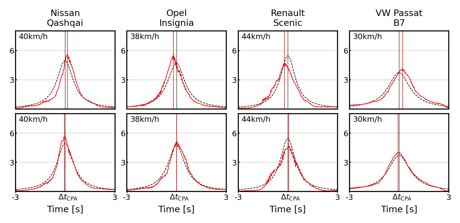
Figure 3: Predicted MA features (solid red) compared to their ground-truth (dashed black). The offset between the ground-truth and the predicted CPA instants (vertical lines), $\Delta t_{\text{CPA}}$, represents labeling noise. Top: MA predictions using original labels. Bottom: MA predictions after label correction is implemented.

Generalization of the proposed MA regression is degraded due to imprecise $t_{\text{CPA}}$ labeling. Since the true $t_{\text{CPA}}$ value cannot be determined precisely by analyzing the video-recording (camera view angle is not known), we propose to correct the ground-truth $t_{\text{CPA}}$ by using the predicted MA profiles of the test data. More precisely, for each audio file, the corrected $t_{\text{CPA}}$ is calculated as a median $t_{\text{CPA}}$ over $20$ runs of the proposed MA regression model. For the $t_{\text{CPA}}$ correction, we consider only the test results of MA regression. Since the test data correspond to a vehicle not included in the training phase, the regression model does not overfit to the test data. After the labels are corrected, the model is trained again. Improvements in $t_{\text{CPA}}$ predictions, due to the proposed label correction, are depicted in Fig. 3 (bottom). Speed estimation improvements are presented in Section IV.

IV Experiments and Results

The proposed method is evaluated in terms of vehicle detection and vehicle speed estimation accuracy. Since vehicle detection is defined as estimation of the $t_{\text{CPA}}$ instant, we calculate detection error as a difference between the true and the estimated MA maxima positions. Distribution (histogram) of MA maxima detection offsets of the test data are presented in Fig. 4 (top). The histogram comprises the test results from $20$ DNN training iterations. If the error is modeled as a normal random variable, its mean value and standard deviation are improved with respect to [7], from $-0.016$ to $-0.009$ and from $0.065$ to $0.053$, respectively. In Fig. 4 (bottom), we compared histograms of the MA maxima values in two scenarios, with vehicle (blue histogram) and without vehicle (orange histogram) passing by the microphone. The width of the green rectangle area, which separates the vehicle and no-vehicle cases, increased from $0.30$, obtained in [7], to $0.45$. This area represents the optimal range to set the MA magnitude threshold for accurate vehicle detection.

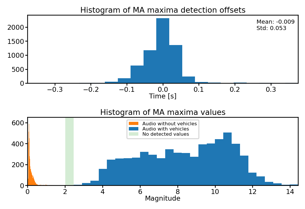
Figure 4: Top: Histogram of MA maxima detection offsets on the test dataset. Bottom: Histogram of MA maxima for audio with vehicles (blue) and without vehicles (orange). Green rectangle separates the two cases.

TABLE I: Speed estimation RMSE

Vehicle	RMSE [km/h]
Citroen C4 Picasso	$6.40$
Mazda 3 Skyactive	$8.57$
Mercedes AMG 550	$6.89$
Nissan Qashqai	$6.21$
Opel Insignia	$4.25$
Peugeot 307	$6.65$
Peugeot 3008	$7.37$
Renault Captur	$5.81$
Renault Scenic	$10.52$
VW Passat B7	$6.50$
Average	$6.92$

TABLE II: Speed classification accuracy with $\Delta$ denoting the distance from the true class

Vehicle	$\Delta=0$	$|\Delta|=1$	$|\Delta|=2$	$|\Delta|>2$	$|\Delta|\leq 1$
Citroen C4 Picasso	$62.6\%$	$28.9\%$	$8.5\%$	$0.0\%$	$91.5\%$
Mazda 3 Skyactive	$43.9\%$	$48.3\%$	$6.2\%$	$1.6\%$	$92.2\%$
Mercedes AMG 550	$50.2\%$	$48.5\%$	$1.3\%$	$0.0\%$	$98.7\%$
Nissan Qashqai	$42.4\%$	$55.2\%$	$2.4\%$	$0.0\%$	$97.6\%$
Opel Insignia	$69.8\%$	$30.2\%$	$0.0\%$	$0.0\%$	$100.0\%$
Peugeot 307	$62.2\%$	$31.0\%$	$6.6\%$	$0.2\%$	$93.3\%$
Peugeot 3008	$48.7\%$	$41.8\%$	$8.5\%$	$1.0\%$	$90.5\%$
Renault Captur	$61.7\%$	$33.3\%$	$5.0\%$	$0.0\%$	$95.0\%$
Renault Scenic	$44.9\%$	$42.3\%$	$8.7\%$	$4.1\%$	$87.1\%$
VW Passat B7	$52.0\%$	$45.4\%$	$2.6\%$	$0.0\%$	$97.4\%$
Average	$53.8\%$	$40.5\%$	$5.0\%$	$0.7\%$	$94.3\%$

Speed estimation accuracy is evaluated using root-mean-square error (RMSE)

$$\text{RMSE}=\sqrt{\frac{1}{L}\sum\nolimits_{l=1}^{L}(v_{l}^{est}-v_{l}^{true})^{2}},$$ (2)

with $v_{l}^{est}$ and $v_{l}^{true}$ representing the estimated and true speeds of the $l$-th measurement, respectively, whereas $L$ is the total number of speed measurements. Average RMSE values, presented in Table I, demonstrate the effect of $t_{\text{CPA}}$ label correction in the training dataset. Compared with [7], the total average RMSE value decreases from $7.39$ km/h to $6.92$ km/h. Vehicle-by-vehicle RMSE comparison with Table II in [7] shows performance improvement for each vehicle except for Opel Insignia, where RMSE is slightly increased.

Speed estimation accuracy is also evaluated in a classification framework. Namely, vehicle speeds are divided into $8$ classes, starting from $25$ km/h, with a step of $10$ km/h. Speed classification results are presented in Table II, with $\Delta$ denoting the distance from the true class. The presented results show improvements of average speed classification accuracies in the cases of $\Delta=0$ (true and predicted classes coincide) and $|\Delta|\leq 1$ (true and predicted classes are adjacent ones) from $53.2\%$ to $53.8\%$ and from $93.4\%$ to $94.3\%$, respectively. Note that the presented speed classification results of Renault Scenic and Mazda 3 Skyactive are highly affected by a background environmental noise during dataset acquisition. On the other hand, Opel Insignia outperforms the other vehicles with the outstanding $|\Delta|\leq 1$ accuracy of $100.0\%$.

V Conclusion

In the paper, we considered how the test results of intermediate MA feature regression could be used to improve coarse labels, obtained by visual scene inspection. The proposed label correction method improved the average speed estimation error by $0.47$ km/h. When formulated as a classification problem, with the discretization interval of $10$ km/h, the achieved accuracy improved $0.6\%$ for correct class prediction and $0.9\%$ in the case when one class offset is allowed.

Our future vehicle speed estimation research will focus on data-oriented approaches such as data augmentation and extending the dataset with additional vehicles.

References

- [1] M. Won, “Intelligent traffic monitoring systems for vehicle classification: A survey,” IEEE Access, vol. 8, pp. 73 340–73 358, 2020.
- [2] H. Shokravi, H. Shokravi, N. Bakhary, M. Heidarrezaei, S. S. Rahimian Koloor, and M. Petru, “A review on vehicle classification and potential use of smart vehicle-assisted techniques,” Sensors, vol. 20, no. 11, p. 3274, 2020.
- [3] S. Djukanović, J. Matas, and T. Virtanen, “Robust audio-based vehicle counting in low-to-moderate traffic flow,” in 2020 IEEE Intelligent Vehicles Symposium (IV). IEEE, 2020, pp. 1608–1614.
- [4] S. Djukanović, Y. Patel, J. Matas, and T. Virtanen, “Neural network-based acoustic vehicle counting,” in 29th European Signal Processing Conference (EUSIPCO 2021), 2021.
- [5] R. Velazquez-Pupo et al., “Vehicle detection with occlusion handling, tracking, and oc-svm classification: A high performance vision-based system,” Sensors, vol. 18, no. 2, p. 374, 2018.
- [6] M. Simoncini, L. Taccari, F. Sambo, L. Bravi, S. Salti, and A. Lori, “Vehicle classification from low-frequency gps data with recurrent neural networks,” Transportation Research Part C: Emerging Technologies, vol. 91, pp. 176–191, 2018.
- [7] S. Djukanović, J. Matas, and T. Virtanen, “Acoustic vehicle speed estimation from single sensor measurements,” IEEE Sensors Journal, vol. 21, no. 20, pp. 23 317–23 324, 2021.
- [8] N. Bulatović and S. Djukanović, “Mel-spectrogram features for acoustic vehicle detection and speed estimation,” in 26th International Scientific-Professional Conference on Information Technology (IT 2022). Žabljak, Montenegro: IEEE, Feb. 16–19, 2022.
- [9] Z. Sun and X. J. Ban, “Vehicle classification using gps data,” Transportation Research Part C: Emerging Technologies, vol. 37, pp. 102–117, 2013.
- [10] M. A. Manzoor and Y. Morgan, “Vehicle make and model recognition using random forest classification for intelligent transportation systems,” in 2018 IEEE 8th Annual Computing and Communication Workshop and Conference (CCWC). IEEE, 2018, pp. 148–154.
- [11] S. Ghassemi, A. Fiandrotti, E. Caimotti, G. Francini, and E. Magli, “Vehicle joint make and model recognition with multiscale attention windows,” Signal Processing: Image Communication, vol. 72, pp. 69–79, 2019.
- [12] M. Biglari, A. Soleimani, and H. Hassanpour, “A cascaded part-based system for fine-grained vehicle classification,” IEEE Transactions on Intelligent Transportation Systems, vol. 19, no. 1, pp. 273–283, 2017.
- [13] N. Almaadeed, M. Asim, S. Al-Maadeed, A. Bouridane, and A. Beghdadi, “Automatic detection and classification of audio events for road surveillance applications,” Sensors, vol. 18, no. 6, p. 1858, 2018.
- [14] P. Foggia, N. Petkov, A. Saggese, N. Strisciuglio, and M. Vento, “Audio surveillance of roads: A system for detecting anomalous sounds,” IEEE transactions on intelligent transportation systems, vol. 17, no. 1, pp. 279–288, 2015.
- [15] M. Naphade et al., “The 2019 AI City challenge,” in CVPR Workshops, 2019, pp. 452–460.
- [16] B. T. Morris and M. M. Trivedi, “A survey of vision-based trajectory learning and analysis for surveillance,” IEEE Transactions on Circuits and Systems for Video Technology, vol. 18, no. 8, pp. 1114–1127, 2008.
- [17] M. Crocco, M. Cristani, A. Trucco, and V. Murino, “Audio surveillance: A systematic review,” ACM Computing Surveys (CSUR), vol. 48, no. 4, pp. 1–46, 2016.
- [18] C. Wilson, C. Willis, J. K. Hendrikz, R. Le Brocque, and N. Bellamy, “Speed cameras for the prevention of road traffic injuries and deaths,” Cochrane database of systematic reviews, no. 11, 2010.
- [19] B. Quinn, “Doppler speed and range estimation using frequency and amplitude estimates,” The Journal of the Acoustical Society of America, vol. 98, no. 5, pp. 2560–2566, 1995.
- [20] C. Couvreur and Y. Bresler, “Doppler-based motion estimation for wide-band sources from single passive sensor measurements,” in 1997 IEEE International Conference on Acoustics, Speech, and Signal Processing, vol. 5. IEEE, 1997, pp. 3537–3540.
- [21] V. Cevher, R. Chellappa, and J. H. McClellan, “Vehicle speed estimation using acoustic wave patterns,” IEEE Transactions on Signal Processing, vol. 57, no. 1, pp. 30–47, 2008.
- [22] S. Barnwal, R. Barnwal, R. Hegde, R. Singh, and B. Raj, “Doppler based speed estimation of vehicles using passive sensor,” in 2013 IEEE International Conference on Multimedia and Expo Workshops (ICMEW). IEEE, 2013, pp. 1–4.
- [23] E. Kubera, A. Wieczorkowska, A. Kuranc, and T. Słowik, “Discovering speed changes of vehicles from audio data,” Sensors, vol. 19, no. 14, p. 3067, 2019.
- [24] H. V. Koops and F. Franchetti, “An ensemble technique for estimating vehicle speed and gear position from acoustic data,” in 2015 IEEE International Conference on Digital Signal Processing (DSP). IEEE, 2015, pp. 422–426.
- [25] J. Giraldo-Guzmán, A. G. Marrugo, and S. H. Contreras-Ortiz, “Vehicle speed estimation using audio features and neural networks,” in 2016 IEEE ANDESCON. IEEE, 2016, pp. 1–4.
- [26] H. Göksu, “Vehicle speed measurement by on-board acoustic signal processing,” Measurement and Control, vol. 51, no. 5-6, pp. 138–149, 2018.
- [27] R. López-Valcarce, C. Mosquera, and F. Pérez-González, “Estimation of road vehicle speed using two omnidirectional microphones: A maximum likelihood approach,” EURASIP Journal on Advances in Signal Processing, vol. 2004, no. 8, p. 929146, 2004.
- [28] K. W. Lo and B. G. Ferguson, “Broadband passive acoustic technique for target motion parameter estimation,” IEEE Transactions on aerospace and electronic systems, vol. 36, no. 1, pp. 163–175, 2000.
- [29] P. Marmaroli, J. Odobez, X. Falourd, and H. Lissek, “Pass-by noise acoustic sensing for estimating speed and wheelbase length of two-axle vehicles,” in Proceedings of Meetings on Acoustics ICA2013, vol. 19. Acoustical Society of America, 2013.
- [30] C. Zhang, S. Bengio, M. Hardt, B. Recht, and O. Vinyals, “Understanding deep learning (still) requires rethinking generalization,” Communications of the ACM, vol. 64, no. 3, pp. 107–115, 2021.
- [31] H. Song, M. Kim, D. Park, Y. Shin, and J.-G. Lee, “Learning from noisy labels with deep neural networks: A survey,” arXiv preprint arXiv:2007.08199, 2020.
- [32] R. Serizel, V. Bisot, S. Essid, and G. Richard, “Acoustic features for environmental sound analysis,” in Computational Analysis of Sound Scenes and Events. Springer, 2018, pp. 71–101.
- [33] C. C. Chang and C. J. Lin, “LIBSVM: A library for support vector machines,” ACM Transactions on Intelligent Systems and Technology (TIST), vol. 2, no. 3, pp. 1–27, 2011.
- [34] L. Stanković, I. Djurović, S. Stanković, M. Simeunović, S. Djukanović, and M. Daković, “Instantaneous frequency in time–frequency analysis: Enhanced concepts and performance of estimation algorithms,” Digital Signal Processing, vol. 35, pp. 1–13, 2014.