Energetics and scattering of gravitational two-body systems at fourth post-Minkowskian order

Abstract

Upcoming observational runs of the LIGO-Virgo-KAGRA collaboration, and future gravitational-wave (GW) detectors on the ground and in space, require waveform models more accurate than currently available. High-precision waveform models can be developed by improving the analytical description of compact binary dynamics and completing it with numerical-relativity (NR) information. Here, we assess the accuracy of the recent results for the fourth post-Minkowskian (4PM) conservative dynamics through comparisons with NR simulations for the circular-orbit binding energy and for the scattering angle. We obtain that the 4PM dynamics gives better agreement with NR than the 3PM dynamics, and that while the 4PM approximation gives comparable results to the third post-Newtonian (PN) approximation for bound orbits, it performs better for scattering encounters. Furthermore, we incorporate the 4PM results in effective-one-body (EOB) Hamiltonians, which improves the disagreement with NR over the 4PM-expanded Hamiltonian from $\sim 40\%$ to $\sim 10\%$, or $\sim 3\%$ depending on the EOB gauge, for an equal-mass binary, two GW cycles before merger. Finally, we derive a 4PN-EOB Hamiltonian for hyperbolic orbits, and compare its predictions for the scattering angle to NR, and to the scattering angle of a 4PN-EOB Hamiltonian computed for elliptic orbits.

I Introduction

Gravitational-wave (GW) observations [1, 2, 3, 4] have improved our understanding of compact binaries, composed of black holes and/or neutron stars, their properties, and their astrophysical formation channels [5, 6, 7]. Searching for GW signals and estimating their parameters require accurate waveform models or templates. Since numerical-relativity (NR) simulations are computationally expensive, analytical approximation methods become essential for producing such waveforms.

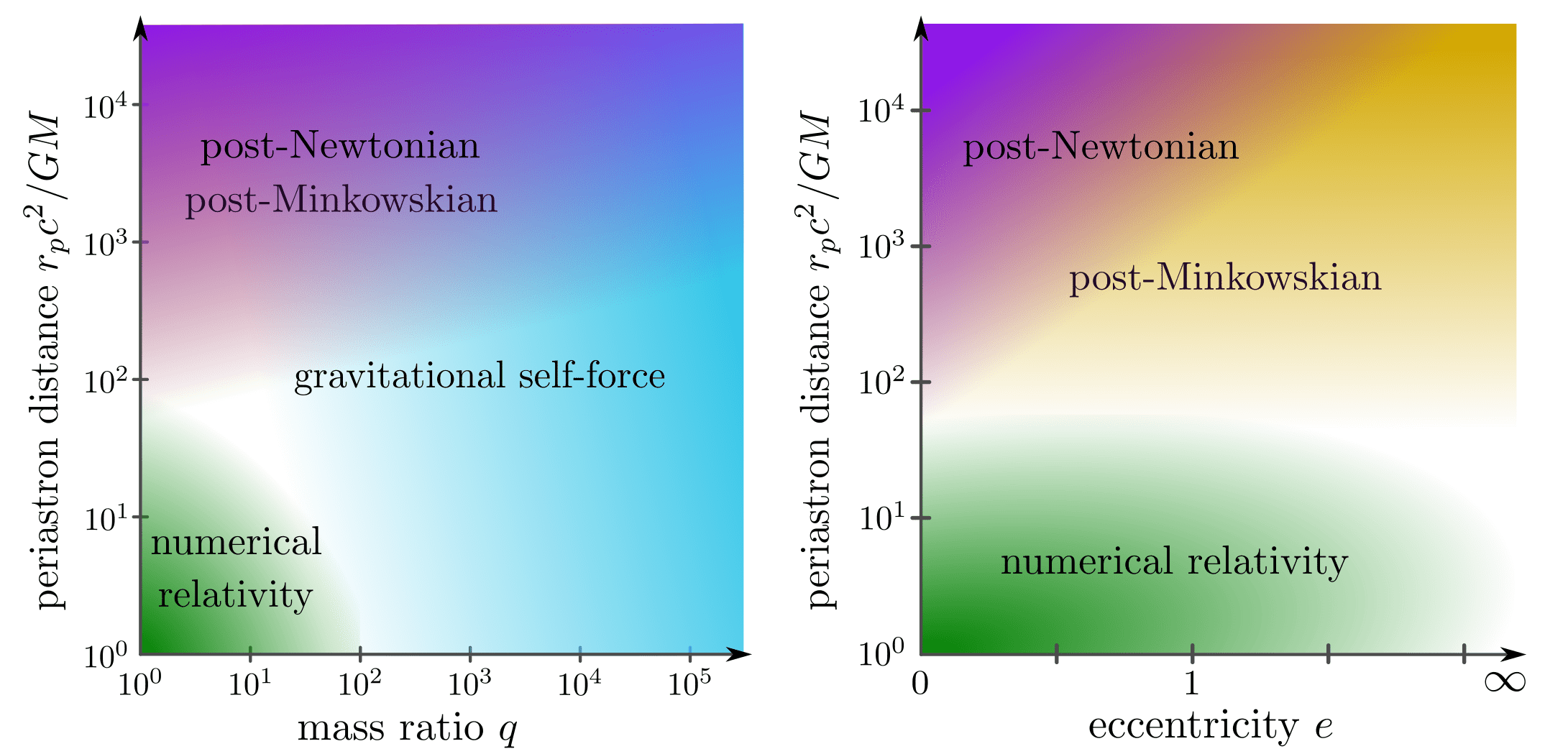
Figure 1: The left panel shows the region of applicability of NR and the PN, PM, and GSF approximations for small eccentricity $e\sim 0$, in which case the PN and PM approximations overlap. The right panel shows the range in eccentricity for which each approximation is applicable for comparable masses $q\sim 1$. The PM approximation is more accurate than the PN approximation for scattering encounters at large velocities, or equivalently large eccentricities at fixed periastron distance.

The post-Newtonian (PN) approximation is valid for slow motion, $v^{2}/c^{2}\ll 1$, and weak gravitational potential, $GM/rc^{2}\ll 1$, making it most applicable for binaries in bound orbits where $v^{2}/c^{2}\sim GM/rc^{2}$, which are the main sources observed by ground-based GW detectors, such as LIGO, Virgo and KAGRA [8, 9, 10]; for reviews, see Refs. [11, 12, 13, 14, 15, 16].

Similarly, the post-Minkowskian (PM) approximation is a weak-field expansion, but places no restriction on the magnitude of velocities. Next to entirely classical approaches to the PM approximation [17, 18, 19, 20, 21, 22, 23, 24, 25], recent progress has been pioneered by methods starting out from (quantum) scattering amplitudes [26, 27, 28, 29, 30, 31, 32, 33, 34, 35, 36, 37, 38, 39]. In addition, manifestly classical methods that make use of quantum-field-theory techniques show great promise for advancing the PM approximation, namely effective field theory [40, 41, 42, 43, 44, 45] and worldline quantum field theory [46, 47] approaches. The PM approximation has also been applied to spin [48, 49, 50, 51, 52, 53, 54, 55, 56, 57, 58, 59, 60, 61, 62, 63, 64, 65, 66, 67], tidal [68, 69, 70, 71, 72, 73, 74, 75], and radiative effects [76, 77, 78, 79, 80, 81, 82, 83, 84, 85, 86, 87, 88, 89, 90].

The PM expansion encompasses the PN expansion, such that the $(n+1)$PM order includes all the information up to the $n$PN order, making it potentially more accurate. Binaries in bound orbits can reach velocities on the order of $0.4$ or larger when spiraling over the last orbits before merger. This means that the relativistic corrections become more and more important in the last stages of the inspiral and plunge. Thus, we might expect that at some high PM order, the PM expansion may start to become more accurate than the PN expansion. Furthermore, scattering encounters on hyperbolic trajectories can reach high velocities, for which the PM approximation becomes more relevant. The gravitational self-force (GSF) approximation [91, 92, 93, 94, 95, 96, 97, 98, 99, 100, 101, 102, 103] expands the Einstein equations in power of the binary’s mass ratio $m_{2}/m_{1}\ll 1$. It is thus valid for any velocity and is not restricted to the weak fields. Figure 1 illustrates the regions of parameter space in which the PN, PM and GSF approximations are (roughly) applicable when generic orbits are considered.

Detecting GW bursts from hyperbolic encounters would have important implications on our understanding of dense stellar environments and the merger rate of compact objects formed through this astrophysical channel. Currently, there does not seem to be a consensus in the literature [104, 105, 106, 107, 108, 109, 110] on the event rate for scattering encounters, due to the high uncertainty in the astrophysical models; the expected event rates vary between 0.001 to 0.39 per year for upcoming LIGO-Virgo-KAGRA runs, depending on the model [110], with higher rates expected for future detectors. Gravitational waves from hyperbolic encounters would be expected at higher rates in the LIGO-Virgo-KAGRA frequency band if a large population of primordial black holes exists in dense stellar clusters, as was proposed in Refs. [111, 112, 113, 114] based on some inflationary models. Other GW sources that could reach highly-relativistic velocities are binaries in galactic nuclei, where dynamical capture and three-body interactions can drive binaries to high eccentricities [106, 115, 116, 117, 118, 119, 120, 121, 122, 123, 124, 125].

Most studies of hyperbolic and parabolic encounters use the PN approximation, for both the dynamics [126, 127, 128, 129] and the GW energy spectrum [107, 130, 131, 132, 133]. The effective-one-body (EOB) formalism [134, 135] has also been applied to scattering, as in Refs. [136, 137, 138, 139, 140, 141]. EOB waveform models improve the inspiral-merger-ringdown waveforms by combining test-body, PN, black-hole perturbation, and NR results. PM results have been incorporated in EOB Hamiltonians in Refs. [22, 23, 142, 143].

In this paper, we study the results of Refs. [34, 35, 44, 45] for the 4PM conservative dynamics, both the “vanilla” 4PM Hamiltonians and the EOB Hamiltonians constructed with 4PM conservative information. Generally, the waveform models are evaluated on the two-body dynamics, which is derived from the Hamiltonian and the radiation-reaction (RR) force. The Hamiltonian describes the conservative dynamics, while the RR force accounts for the energy and angular momentum losses due to GWs, and it is included in the right-hand side of the Hamilton equations. Since the RR force has not been computed in PM theory at sufficiently high PM order, in this paper, we restrict our study to the conservative sector, and therefore focus on the Hamiltonian. As shown in Refs. [144, 145, 146], a good diagnostic to assess the accuracy of models for the conservative dynamics is to compare the binding energy from the Hamiltonians and NR. The latter contains both conservative and dissipative effects. When augmenting the models’ dynamics with RR effects, the binding energy can change (e.g., see Fig. 6 in Ref. [142]). However, it is still very informative to perform studies that compare to NR only the conservative dynamics at various orders of the perturbative expansion, and also develop different flavors of Hamiltonians, and explore their closeness to NR. Eventually, when RR effects in PM theory become available, one will be able to identify the most suitable model for the full dynamics that best represent the NR results. Quite interestingly, in the case of the scattering angle, for which we can add the RR effects to the models’ predictions, we show that the radiative contribution is much smaller than the conservative one (see Fig. 6 below).

The paper is structured as follows. In Sec. II and Sec. III, we summarize the 4PM results and incorporate them in EOB Hamiltonians. Then, in Sec. IV, we compare the circular-orbit binding energies with NR, while in Sec. V, we compare the scattering angles. We conclude in Sec. VI, and write in Appendices A and B the expressions for the PN and EOB Hamiltonians. We also provide those expressions as a Mathematica file in the Supplemental Material [147].

Notation

We adopt units in which the speed of light $c=1$.

For a binary with masses $m_{1}$ and $m_{2}$, with $m_{1}\geq m_{2}$, we define the following quantities:

$$M\equiv m_{1}+m_{2},\quad\mu\equiv\frac{m_{1}m_{2}}{M},\quad\nu\equiv\frac{\mu}{M},\quad q\equiv\frac{m_{1}}{m_{2}}.$$ (1)

From the total energy $E$, we define the binding energy:

$$\bar{E}\equiv\frac{E-M}{\mu},$$ (2)

and the effective energy $E_{\text{eff}}$ through the EOB energy map [134]

$$E=M\sqrt{1+2\nu\left(\frac{E_{\text{eff}}}{\mu}-1\right)}\,.$$ (3)

We also introduce the following quantities:

$$\gamma \equiv\frac{E_{\text{eff}}}{\mu}=\frac{E^{2}-m_{1}^{2}-m_{2}^{2}}{2m_{1}m_{2}},$$

$$\Gamma \equiv\frac{E}{M}=\sqrt{1+2\nu(\gamma-1)}\,,$$ (4)

where $\gamma$ is related to the asymptotic relative velocity $v$ by

$$v\equiv\frac{\sqrt{\gamma^{2}-1}}{\gamma},\quad\text{or}\quad\gamma=\frac{1}{\sqrt{1-v^{2}}}.$$ (5)

When dealing with PN expansions, it is convenient to define the dimensionless energy variable

$$\varepsilon\equiv\gamma^{2}-1=\gamma^{2}v^{2}.$$ (6)

The orbital angular momentum is denoted $L$, and is related to the relative position $R$, radial momentum $P_{R}$, and total linear momentum $P$ via

$$P^{2}=P_{R}^{2}+\frac{L^{2}}{R^{2}}.$$ (7)

We use $H_{\text{hyp}}$ to denote a Hamiltonian with PM or PN information that is valid for unbound/hyperbolic motion, and use $H_{\text{ell}}$ for a Hamiltonian valid for bound/elliptic orbits. A Hamiltonian written without a ‘hyp’ or ‘ell’ subscript is valid for generic motion.

We often use the following dimensionless rescaled quantities:

$$r\equiv\frac{R}{GM},\quad u\equiv\frac{1}{r},\quad p\equiv\frac{P}{\mu},\quad p_{r}\equiv\frac{P_{R}}{\mu},$$

$$l\equiv\frac{L}{GM\mu},\quad\hat{H}\equiv\frac{H}{\mu}.$$ (8)

II PM-expanded scattering angle and Hamiltonian

The 4PM conservative dynamics (including tail effects) has been derived recently in Refs. [34, 35, 44, 45] for hyperbolic orbits in a large-eccentricity expansion. We note that this 4PM result agrees with the 6PN result of Refs. [82, 149, 150], and exhibits a simple mass dependence, which is expected due to Lorentz invariance and dimensional analysis, as argued in Ref. [24]. The result of Refs. [34, 35, 44, 45] also agrees with the 5PN result of Refs. [151, 152, 153], except for a single term that does not have the expected mass dependence, and is proportional to $\nu^{2}$.  Furthermore, Ref. [45] argued that conservative memory terms are still missing at 4PM order. However, at the PM order we are considering, there is no unique definition of the conservative dynamics. In this paper, we follow the definition of the conservative dynamics of Refs. [82, 149, 150], which implies that memory effects at 4PM order will appear in the dissipative dynamics, and will be accounted for when they become available. Thus, here we assume that the conservative-dynamics results in Refs. [34, 35, 44, 45] are complete.

The two-body dynamics can be conveniently encoded in the gauge-invariant radial action, $I_{r}$, which at 4PM order can be written schematically as

$$I_{r,\text{4PM}}^{\text{hyp}} =I_{r,\text{3PM}}-\frac{\pi G^{4}M^{7}\nu^{2}P^{2}}{8EL^{3}}\Bigg{[}\mathcal{M}_{4}^{\text{p}}$$

$$+\nu\left(4\mathcal{M}_{4}^{\text{t}}\ln\frac{\sqrt{\gamma^{2}-1}}{2}+\mathcal{M}_{4}^{\pi^{2}}+\mathcal{M}_{4}^{\text{rem}}\right)\Bigg{]},$$ (9)

which includes the lower PM orders, with the 3PM part $I_{r,\text{3PM}}$ valid for both bound and unbound motion. The terms $\mathcal{M}_{4}^{\dots}$ are directly related to parts of the scattering amplitude; they are independent of the masses, and are written in Eq. (3) of Ref. [35]. An expression for these terms that is valid for generic orbits (bound and unbound) is difficult to derive and has not yet been found. The physical reason is that the tail effects [154] start to enter at 4PM order, which is a nonlocal-in-time interaction depending on the entire history of the binary. Thus, it is different for bound and unbound orbits.

The scattering angle, by which the two bodies are deflected in the center-of-mass frame, is a gauge-invariant function that contains the same information as the radial action or the hyperbolic-orbit Hamiltonian. It can be obtained from the derivative of the radial action with respect to the angular momentum, that is,

$$\chi=-\frac{\partial I_{r}^{\text{hyp}}}{\partial L}-\pi.$$ (10)

The 3PM and 4PM pieces of the conservative scattering angle have a logarithmic divergence in the high-energy (massless) limit. However, that divergence at 3PM order was shown to cancel with a corresponding divergence in the radiative contribution [76, 77, 78, 79, 80, 81], and it is expected that such divergence also cancels at 4PM order [82]. In this paper, we only consider comparable-mass binaries, for which the singularity in the massless limit is irrelevant, and we demonstrate in Fig. 6 that the radiative contribution to the 3PM scattering angle is negligible for the range of parameters we consider.

Reference [35] also derived a two-body Hamiltonian from the radial action, following the steps in Refs. [29, 155]. The 4PM Hamiltonian in isotropic gauge, and for hyperbolic orbits, is given by

$$H_{\text{4PM}}^{\text{hyp}}=\sqrt{m_{1}^{2}+P^{2}}+\sqrt{m_{2}^{2}+P^{2}}+\sum_{n=1}^{4}\frac{G^{n}}{R^{n}}c_{n},$$ (11)

where the $c_{n}$ coefficients are given by Eqs. (10) of Ref. [31] and Eq. (8) of Ref. [35]. Like the radial action, the 3PM part of $H_{\text{4PM}}^{\text{hyp}}$ is valid for generic motion, but the 4PM piece is for hyperbolic orbits. This Hamiltonian is determined in Ref. [35] from an ansatz that matches the scattering angle that follows from the radial action $I_{r,\text{4PM}}^{\text{hyp}}$, which is determined from the scattering amplitude.

To assess how close $H_{\text{4PM}}^{\text{hyp}}$ is to a bound-orbit 4PM Hamiltonian, we complement $H_{\text{4PM}}^{\text{hyp}}$ with bound-orbit corrections $\Delta H_{\text{4PM(nPN)}}^{\text{ell}}$, such that the $n$PN expansion of $H_{\text{4PM}}^{\text{hyp}}+\Delta H_{\text{4PM(nPN)}}^{\text{ell}}$ gives the correct $n$PN Hamiltonian up to $\operatorname{\mathcal{O}}(G^{4})$ for bound orbits in isotropic gauge. We obtain $\Delta H_{\text{4PM(nPN)}}^{\text{ell}}$ to 6PN order, as explained in Appendix A, since the 6PN Hamiltonian is fully known up to $\operatorname{\mathcal{O}}(G^{4})$ [149, 150]. In Sec. IV, we compare the binding energy calculated from these Hamiltonians with NR, finding a small difference between $H_{\text{4PM}}^{\text{hyp}}$ and its bound-orbit corrections.

III Effective-one-body Hamiltonians

In the case of nonspinning compact objects, the EOB formalism [134, 135] maps the binary motion to that of a test mass in a deformed Schwarzschild background. The two-body Hamiltonian $H^{\text{EOB}}$ is related to an effective Hamiltonian $H^{\text{eff}}$ via the energy map

$$H^{\text{EOB}}=M\sqrt{1+2\nu\left(\frac{H_{\text{eff}}}{\mu}-1\right)}\,.$$ (12)

The effective metric is defined by

$$g_{\mu\nu}^{\text{eff}}\mathrm{d}x^{\mu}\mathrm{d}x^{\nu}=-A\mathrm{d}T^{2}+B\mathrm{d}R^{2}+R^{2}\left(\mathrm{d}\theta^{2}+\sin^{2}\theta\mathrm{d}\phi^{2}\right),$$ (13)

with the mass-shell condition [156]

$$0=g^{\mu\nu}_{\text{eff}}P_{\mu}P_{\nu}+\mu^{2}+Q,$$ (14)

leading to the effective Hamiltonian $H_{\text{eff}}=-P_{0}$,

$$H_{\text{eff}}^{2}=A\left(\mu^{2}+\frac{P_{R}^{2}}{B}+\frac{L^{2}}{R^{2}}+Q\right).$$ (15)

In the $\nu\to 0$ limit, $H_{\text{eff}}$ reduces to the Schwarzschild Hamiltonian for a test mass, which is given by

$$\hat{H}_{S}^{2}=(1-2u)\left[1+(1-2u)p_{r}^{2}+l^{2}u^{2}\right].$$ (16)

To include higher PN information in an EOB Hamiltonian, we write an ansatz for the $A,B$ and $Q$ potentials in Eq. (15), perform a canonical transformation, then match $H^{\text{EOB}}$ to the PN-expanded Hamiltonian. This procedure is explained in more detail in Appendix A. For PM results, it is more convenient to calculate the gauge-invariant scattering angle from the ansatz for $H^{\text{EOB}}$, then match it to the PM-expanded scattering angle in Eq. (10). These calculations will lead to the first derivation of 4PM-EOB Hamiltonians (and their $n$PN limits) for hyperbolic orbits.

As an ansatz, we choose the $B$ potential to be the same as in the Schwarzschild metric, i.e., $B=1/(1-2u)$, and include all the 4PM corrections into either $Q$ or $A$. When included in $Q$, we get a 4PM generalization of the post-Schwarzschild (PS) Hamiltonian considered in Refs. [23, 142], which is given by

$$(\hat{H}^{\text{eff,PS}})^{2}=\hat{H}_{S}^{2}+(1-2u)$$

$$\qquad\times\left(u^{2}q_{\text{2PM}}+u^{3}q_{\text{3PM}}+u^{4}q_{\text{4PM}}+\Delta_{\text{4PN}}^{Q}\right),$$ (17)

where $q_{n\text{PM}}$ can in general be any scalar function of the energy or the dynamical variables. In this ansatz, we include a 4PN correction term $\Delta_{\text{4PN}}^{Q}$ as explained below.

The other gauge we consider in this paper incorporates PM corrections in the $A$ potential, and reads

$$(\hat{H}^{\text{eff},\text{PS}^{*}})^{2} =\big{(}1-2u+u^{2}a_{\text{2PM}}+u^{3}a_{\text{3PM}}+u^{4}a_{\text{4PM}}$$

$$\qquad+\Delta_{\text{4PN}}^{A}\big{)}\left[1+(1-2u)p_{r}^{2}+l^{2}u^{2}\right],$$ (18)

which is meant to more closely resemble, in the circular-orbit limit, the standard EOB gauge of Refs. [134, 156, 157], which is often used in EOB waveform models for LIGO-Virgo-KAGRA observations.

To determine the $q_{n\text{PM}}$ and $a_{n\text{PM}}$ coefficients, we calculate the scattering angle from the Hamiltonian. To achieve this, we invert the Hamiltonian $\hat{H}^{\text{EOB}}(l,r,p_{r})=\bar{E}+1/\nu$ to obtain $p_{r}(\bar{E},l,r)$, then evaluate the integral

$$\chi=-2\int_{r_{0}}^{\infty}\frac{\partial p_{r}(\bar{E},l,r)}{\partial l}dr-\pi\,,$$ (19)

where $r_{0}$ is the turning point obtained from the largest root of the unperturbed (1PM) radial momentum $p_{r}^{(0)}(\bar{E},l,r)=0$. To simplify evaluating this integral, we assume that a canonical transformation has been performed such that $q_{n\text{PM}}$ and $a_{n\text{PM}}$ are functions only of the effective energy $E_{\text{eff}}$, which is constant. However, since $q_{n\text{PM}}$ and $a_{n\text{PM}}$ themselves define $H_{\text{eff}}$, their dependence on $E_{\text{eff}}$ should be understood perturbatively in the PM scheme. When working up to 3PM order, that energy can be taken to be the (1PM-accurate) Schwarzschild Hamiltonian $\hat{H}_{S}$ (see Refs. [23, 142] for more details). However, at 4PM order, we need to account for nonlinear effects by using the 2PM effective energy, as explained in Appendix B.

Since the scattering angle is gauge invariant, matching $\chi$ calculated from the EOB Hamiltonian to the PM-expanded scattering angle in Eq. (10) enables us to solve for the coefficients $q_{n\text{PM}}(\gamma)$ and $a_{n\text{PM}}(\gamma)$, where $\gamma\equiv E_{\text{eff}}/\mu$. (See Appendix B or the Supplemental Material [147] for the expressions of these coefficients.).

Table 1: Summary of the Hamiltonians considered in this paper.

Hamiltonian	Definition
$H_{n\text{PN}}$	PN-expanded Hamiltonian to $\operatorname{\mathcal{O}}(c^{-2n})$
$H_{n\text{PM}}$	PM-expanded Hamiltonian to $\operatorname{\mathcal{O}}(G^{n})$
$H_{\text{4PM}}^{\text{hyp}}+\Delta H_{\text{4PM}(n\text{PN})}^{\text{ell}}$	4PM hyperbolic-orbit Hamiltonian plus a bound-orbit correction up to orders $n$PN and 4PM
$H_{\text{nPN(4PM)}}^{\text{ell,iso}}$	PN-expanded Hamiltonian truncated at $\operatorname{\mathcal{O}}(G^{4})$ in isotropic coordinates, valid for bound orbits
$H_{n\text{PN}}^{\text{EOB}}$	PN-EOB Hamiltonian in the gauge used in Refs. [157, 134, 156]
$H_{\dots}^{\text{EOB,PS}}$	EOB Hamiltonian in Eq. (III), based on the PS gauge [23, 142]
$H_{\dots}^{\text{EOB},\text{PS}^{*}}$	EOB Hamiltonian in the gauge used in Eq. (III)
$H_{\text{4PM}+\text{4PN}}^{\text{EOB,\ldots}}$	4PM-EOB Hamiltonian (for hyperbolic orbits) complemented with the missing 4PN part (for bound orbits).

We also complement the 4PM EOB Hamiltonians above with the missing 4PN(5PM) piece. This is done by writing an ansatz for $\Delta_{\text{4PN}}$, such that

$$\Delta_{\text{4PN}} =\sum_{n=2}^{5}\alpha_{n}u^{n}\varepsilon^{5-n}+\left(\alpha_{\text{4,ln}}u^{4}\varepsilon+\alpha_{\text{5,ln}}u^{5}\right)\ln u$$

$$\quad+\alpha_{\text{4,ln}\varepsilon}u^{4}\ln\varepsilon,$$ (20)

where we use the PN expansion parameters $u$ and $\varepsilon\equiv\gamma^{2}-1$, each of one PN order. Then, we perform a canonical transformation and match the result to the elliptic 4PN Hamiltonian of Ref. [157]. Note that the $\ln\varepsilon$ term is there to cancel a corresponding term that appears in the 4PM hyperbolic-orbit Hamiltonian. The coefficients in Eq. (III) are written in Appendix B.

We summarize in Table 1 the different Hamiltonians considered in this paper.

IV Binding energy for circular orbits

The 4PM part of the Hamiltonian in Eq. (11) is valid in the large-eccentricity limit, which means it is not consistent with the circular-orbit binding energy at 4PN and higher orders. However, we show that the tail contribution to that Hamiltonian has a small effect on the dynamics, and so we use it to get an estimate for the 4PM contribution to the binding energy.

IV.1 PN-expanded binding energy

We start by comparing the PN-expanded binding energy calculated from a bound-orbit Hamiltonian to the unbound case.

In Appendix A, we compute the bound-orbit 6PN Hamiltonian in isotropic coordinates, by canonically transforming the EOB Hamiltonian of Refs. [149, 150]. We truncate that Hamiltonian at 4PM, and calculate the binding energy, which at 4PN reads

$$\bar{E}_{\text{4PN(4PM)}}^{\text{iso,ell}} =\bar{E}_{\text{3PN}}(x)+x^{5}\bigg{[}\frac{11795}{768}-\nu\frac{518}{45}\ln x$$

$$\quad+\nu\left(\frac{428071\pi^{2}}{36864}-\frac{7899659}{34560}+\frac{1036\ln 2}{45}\right)$$

$$\quad+\nu^{2}\left(\frac{1435\pi^{2}}{576}-\frac{122815}{6912}\right)-\frac{5341\nu^{3}}{3456}$$

$$\quad-\frac{77\nu^{4}}{62208}\bigg{]},$$ (21)

where $\bar{E}_{\text{3PN}}(x)$ is given by Eq. (232) of Ref. [12], and $x\equiv(M\Omega)^{2/3}$, with $\Omega$ being the orbital frequency. Note that the 4PN part of this result is not gauge invariant, but is only valid for isotropic coordinates. The reason is that PN-accurate coordinate transformations—for example to isotropic coordinates—in general span several PM orders.

We find that the difference between the binding energy in Eq. (IV.1) and the energy computed from the hyperbolic-orbit Hamiltonian (11) at 4PN is given by

$$\bar{E}_{\text{4PN(4PM)}}^{\text{iso,hyp}}-\bar{E}_{\text{4PN(4PM)}}^{\text{iso,ell}}$$

$$\qquad=\nu x^{5}\bigg{[}\frac{37933}{45}+\frac{1036\gamma_{E}}{45}-\frac{113847608\ln 2}{45}$$

$$\quad\qquad-\frac{1472499\ln 3}{20}+\frac{13671875\ln 5}{12}\bigg{]}$$

$$\qquad\simeq 14.94\nu x^{5}\,,$$ (22)

where we see that the disagreement is in the non-logarithmic, linear-in-$\nu$ coefficient of Eq. (IV.1). That coefficient is $-112.96$ in $\bar{E}_{\text{4PN(4PM)}}^{\text{iso,ell}}$, and is $-98.01$ in $\bar{E}_{\text{4PN(4PM)}}^{\text{iso,hyp}}$, with the difference being $14.94$. (Note that the $\ln x$ term in Eq. (IV.1) is the same for bound and unbound orbits, as was shown to all PN orders in Ref. [89].)

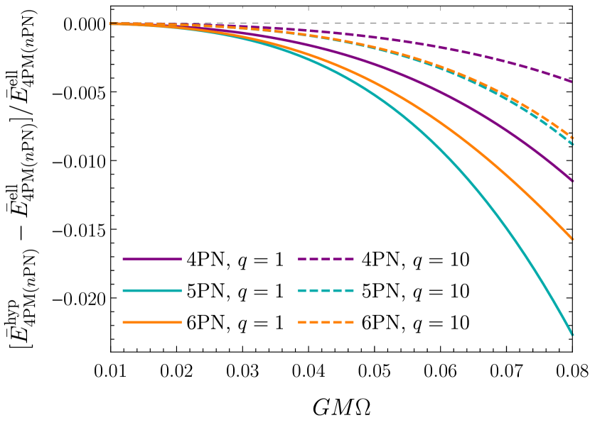
Figure 2: Relative difference in the circular-orbit binding energy, computed analytically from an elliptic versus a hyperbolic-orbit Hamiltonian.

In Fig. 2, we plot the relative difference in the binding energy at different PN orders, and for mass ratios $q=1$ and $q=10$, finding disagreement $\lesssim 2\%$, which justifies applying the hyperbolic 4PM result to bound orbits as we do below, since we find that the disagreement with NR is larger than $2\%$.

IV.2 Binding energy from PM-expanded Hamiltonians

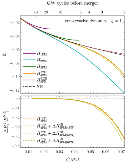
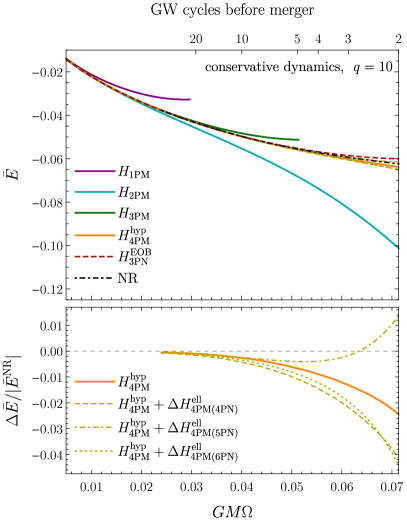
Figure 3: Binding energy versus orbital frequency for the PM-expanded Hamiltonians compared to the NR prediction for a nonspinning equal-mass (left panel) and mass-ratio $q=10$ (right panel) binary black hole. The top axis gives the number of GW cycles before merger, which is twice the number of orbits. The lower panels show the relative difference of the 4PM curves with NR.

To compute the binding energy for circular orbits from the PM-expanded Hamiltonian in Eq. (11), we do so numerically by setting $p_{r}=0$ in the Hamiltonian and solving $\dot{p}_{r}=-\partial\hat{H}/\partial r=0$ for the angular momentum $l$ at different orbital separations. We then plot $\bar{E}=\hat{H}_{n\text{PM}}-1/\nu$ versus the orbital frequency $M\Omega=\partial\hat{H}/\partial l$ (see Ref. [142] for more details).

In Fig. 3, we compare the binding energy with NR data that were extracted in Ref. [158] from numerical simulations produced by the Simulating eXtreme Spacetimes (SXS) collaboration [159, 160]. In particular, we use the simulations with SXS ID 0180 for mass ratio $q=1$ and ID 0303 for $q=10$, for which the numerical error is too small to show in the figure.

We see that the 4PM Hamiltonian gives much better agreement with NR toward merger than Hamiltonians computed at lower PM orders. This is because the 4PM Hamiltonian contains the full 3PN information, which is known to give considerably better results than 2PN. The improvement at 4PM is even more significant for mass ratio $q=10$ than $q=1$, because the 3PN coefficient in the binding energy increases significantly with increasing mass ratio. In addition, it seems that $H_{\text{4PM}}^{\text{hyp}}$ is very close to what a bound-orbit 4PM Hamiltonian would be, as evidenced by how close the curves $H_{\text{4PM}}^{\text{hyp}}+\Delta H_{\text{4PM(nPN)}}^{\text{ell}}$, computed at 4PN, 5PN and 6PN orders, are to $H_{\text{4PM}}^{\text{hyp}}$.

For comparison, the figure also shows the 3PN EOB Hamiltonian in the gauge of Refs. [134, 156, 157], which gives better agreement with NR (also when considering different mass ratios) because it includes the exact test-body limit, and the associated resummation of the PN results. In the plots, we stop the numerical evaluation of the energy either at the innermost-stable circular orbit (ISCO) or at two GW cycles (one orbit) before merger. We note that the EOB results on the figures do not contain any NR information, and the $g_{00}$ effective metric contains PN terms in a Taylor-expanded form.

IV.3 Binding energy from PM-EOB Hamiltonians

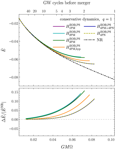
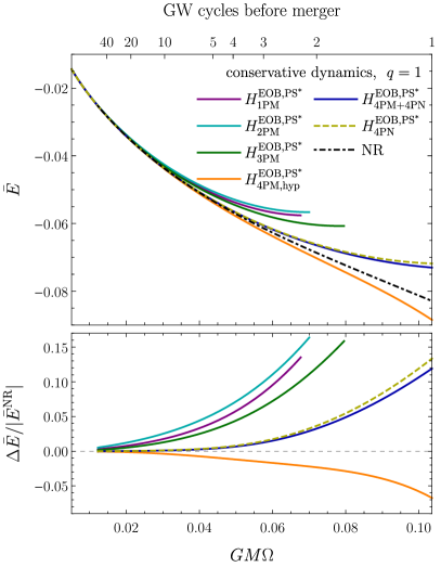
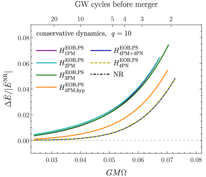
Figure 4: Binding energy versus orbital frequency for the PM-EOB Hamiltonians, compared to the NR prediction for $q=1$. The left panels contain results for the EOB Hamiltonian in the PS gauge in Eq. (III), while the right panels are for the $\text{PS}^{*}~{}$gauge in Eq. (III).

Figure 5: Similar to Fig. 5 but for mass ratio $q=10$, and we only show the relative difference since the EOB curves are closer to the NR curve than for equal masses. All curves end at the ISCO.

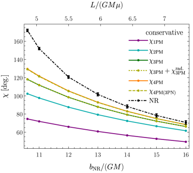
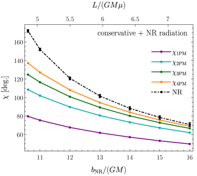
Figure 6: Comparison of the PM-expanded scattering angle with NR. The left panel shows the conservative scattering angle, except for the $\chi_{\text{3PM}}+\chi_{\text{3PM}}^{\text{rad.}}$ curve that also includes the leading-order (3PM) radiative contribution. The right panel incorporates the effect of the radiative losses from the NR simulations using Eq. (25).

Similarly, computing the binding energy from the PM-EOB Hamiltonians leads to Fig. 5 for $q=1$ and Fig. 5 for $q=10$. In both figures, we plot the binding energy at each PM order, and complement 4PM with 4PN information. We stop the numerical evaluation either at the ISCO or at one GW cycle before merger.

From the figures, we observe the following:

• The 4PM order provides a significant improvement over the lower orders, even though the PM Hamiltonian is for hyperbolic orbits.

• The $\text{PS}^{*}~{}$gauge performs better than the PS gauge, for both equal and unequal masses. That difference is due to higher-order terms resulting from the resummation of the Hamiltonian coefficients. We expect that the more PN/PM orders are included, the closer different gauges would be to each other.

• Complementing 4PM with the missing 4PN information for bound orbits gives results for the $\text{PS}^{*}~{}$gauge that are comparable to the standard PN-EOB gauge.

• Using 4PN-expanded potentials in $H_{\text{4PN}}^{\text{EOB,...}}$ gives almost the same result as the 4PM+4PN Hamiltonian, although for the $\text{PS}^{*}~{}$gauge, the 4PM+4PN Hamiltonian is slightly better for equal masses than its 4PN expansion.

V Scattering angle comparison with NR

Since the 4PM part of the radial action in Eq. (II) is valid for hyperbolic orbits, a better comparison with NR is through the scattering angle.

NR simulations for the scattering angle were reported in Ref. [136] for equal masses $q=1$ and initial linear momentum $|\bm{p}|=0.11456439M$. The initial energy in these simulations is approximately $E_{\text{in}}^{\text{NR}}\simeq 1.02259$ (corresponding to velocity $v\simeq 0.4$), and the initial angular momentum $L_{\text{in}}^{\text{NR}}$ is proportional to the impact parameter $b_{\text{NR}}$, which ranges between 9$M$ and 16$M$. The NR error in the scattering angle is $\sim 1-2$ degrees.

Reference [136] also reported the energy and angular momentum losses due to the emitted GWs, which can be used to account for the radiative contribution to the scattering angle. It was proven in Ref. [128] that when working to linear order in RR, the radiative contribution to the total scattering angle is half the difference of the conservative scattering angle evaluated as a function of the outgoing and incoming states, i.e.,

$$\chi^{\text{rad.}}=\frac{1}{2}\left[\chi^{\text{cons.}}(E_{\text{out}},L_{\text{out}})-\chi^{\text{cons.}}(E_{\text{in}},L_{\text{in}})\right],$$ (23)

which means that the total scattering angle is given by

$$\chi^{\text{tot}}(E_{\text{in}},L_{\text{in}})\equiv\chi^{\text{cons.}}(E_{\text{in}},L_{\text{in}})+\chi^{\text{rad.}}(E_{\text{in}},L_{\text{in}})$$

$$\qquad=\frac{1}{2}\left[\chi^{\text{cons.}}(E_{\text{in}},L_{\text{in}})+\chi^{\text{cons.}}(E_{\text{out}},L_{\text{out}})\right],$$ (24)

which can be written as

$$\chi^{\text{tot}}(E_{\text{in}},L_{\text{in}})=\chi^{\text{cons.}}(E_{\text{avg}},L_{\text{avg}}),$$ (25)

where

$$E_{\text{avg}}\equiv\frac{E_{\text{in}}+E_{\text{out}}}{2},\quad L_{\text{avg}}\equiv\frac{L_{\text{in}}+L_{\text{out}}}{2}.$$ (26)

We emphasize that Eq. (25) holds when neglecting contributions quadratic in RR, which start at 5PN order.

V.1 PM-expanded scattering angle

In the left panel of Fig. 6, we plot the conservative PM-expanded scattering angle, calculated from Eq. (10), for the initial values of energy and angular momentum used in the NR simulations, which are written in Table I of Ref. [136]. We see that each PM order gives better agreement with NR than the lower orders, with an overall good agreement at 4PM, especially considering that these scattering angles are rather large while the PM expansion is an approximation away from a straight line.

We also plot the 3PN expansion of the 4PM scattering angle, finding that the difference with the full 4PM angle is only $\sim.1$ degrees. This is because the initial velocity is $v\simeq 0.4$, for which a PN expansion provides a good approximation. Higher velocities would lead to larger differences between the PM scattering angle and its PN expansion. Furthermore, the figure shows the 3PM conservative scattering angle plus the leading order (3PM) radiative contribution, which is given by Eq. (5.7) of Ref. [76]; however, the effect of that radiative contribution is so small that it is almost the same as the conservative 3PM curve.

In the right panel of Fig. 6, we plot the scattering angle taking into account the effect of RR by modifying the initial conditions, as explained above in Eq. (25). We see that all curves are shifted closer to the NR curve, but their order remains the same.

V.2 Scattering angle from PM-EOB Hamiltonians

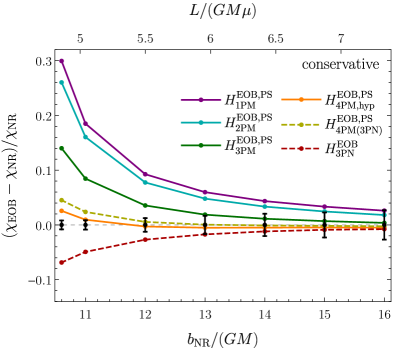
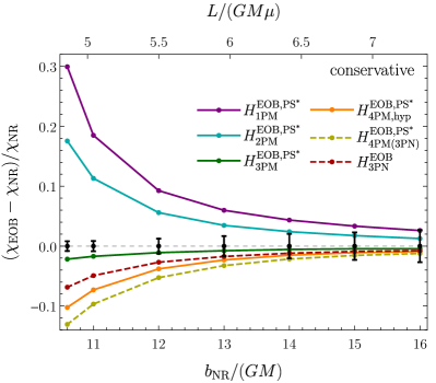
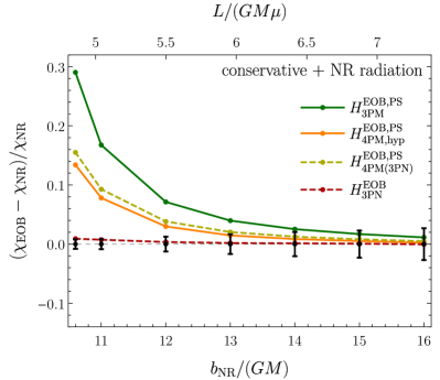
Figure 7: Comparison with NR of the conservative scattering angle computed from the EOB Hamiltonians in the PS gauge (left panel) and the $\text{PS}^{*}~{}$gauge (right panel).

Figure 8: Scattering angle calculated from the EOB Hamiltonians in the PS gauge (left panel) and the $\text{PS}^{*}~{}$gauge (right panel) while incorporating radiative effects from NR through the initial conditions as in Eq. (25).

To compute the scattering angle from the EOB Hamiltonians, we start with an initial azimuthal angle $\phi_{\text{in}}=0$, evolve the equations of motion without RR force, then read off the final angle $\phi_{\text{out}}$, leading to the scattering angle $\chi_{\text{EOB}}=\phi_{\text{out}}-\phi_{\text{in}}-\pi$. We start the evolution with initial separation $r_{\text{in}}=10^{4}$, initial angular momentum $L_{\text{in}}^{\text{NR}}$, and solve $E_{\text{in}}^{\text{NR}}=H^{\text{EOB}}$ for the initial $p_{r}$.

In Fig. 8, we plot the relative difference in the conservative scattering angle between EOB and NR, finding much smaller difference than the PM-expanded angles in Fig. 6. Similarly, in Fig. 8, we plot the same quantity but using initial conditions that account for the NR energy and angular momentum losses, as in Eq. (25). For comparison, both figures show the scattering angle calculated from a 3PN EOB Hamiltonian in the gauge of Refs. [157, 134, 156], which is valid for arbitrary trajectories since 3PN is purely local in time (no tails contributions).

From Fig. 8, we see that 4PM performs better than 3PM for the PS gauge, but 3PM is better for the $\text{PS}^{*}~{}$gauge. However, when including the NR RR in Fig. 8, 4PM becomes closer to NR than 3PM for both gauges. We also see that the $\text{PS}^{*}~{}$gauge gives better agreement with NR than the PS gauge.

For bound orbits, we saw in the previous section that PN-expanding the PM Hamiltonians gave almost the same results. For scattering encounters on the other hand, we see from both Fig. 8 and Fig. 8 that the 4PM Hamiltonians lead to better results than the 3PN expansion of their potentials, for both EOB gauges and whether or not RR is included.

V.3 4PN EOB Hamiltonian for hyperbolic orbits

The 4PN EOB Hamiltonian derived in Ref. [157] included the tail part in a small-eccentricity expansion, and is thus valid for bound orbits. The 4PN tail contribution for hyperbolic orbits was derived in Ref. [161], analytically at leading order in the large-eccentricity expansion, and numerically for eccentricity $\geq 1$. However, it is not straightforward to translate the all-orders-in-eccentricity result of Ref. [161] to an EOB Hamiltonian in the form of Eq. (15). Therefore, here, we compute a hyperbolic-orbit 4PN EOB Hamiltonian at next-to-leading order in the large-eccentricity expansion. We use that Hamiltonian to compare the effect of using an elliptic versus a hyperbolic-orbit Hamiltonian on the scattering angle.

We start by writing an effective Hamiltonian of the form

$$\hat{H}_{\text{eff}}^{\text{4PN,hyp}} =\sqrt{A^{\text{hyp}}\left[1+\frac{p_{r}^{2}}{B^{\text{hyp}}}+l^{2}u^{2}+Q^{\text{hyp}}\right]}\,,$$ (27)

$$(B^{\text{hyp}})^{-1} \equiv A^{\text{hyp}}\bar{D}^{\text{hyp}},$$ (28)

in which the potentials contain local and nonlocal-in-time contributions, starting at 4PN order. The local part is valid for generic motion, and is given by Eqs. (4.4), (9.6) and (9.7) of Ref. [148], which we follow in how the local and nonlocal parts are split.

We then write an ansatz for the potentials with unknown coefficients for the nonlocal contribution, that is

$$A^{\text{hyp}}=1-2u+2\nu u^{3}+\left(\frac{94}{3}-\frac{41}{32}\pi^{2}\right)\nu u^{4}$$

$$\qquad+\left[\left(\frac{41\pi^{2}}{32}-\frac{221}{6}\right)\nu^{2}+\left(\frac{2275\pi^{2}}{512}-\frac{4237}{60}\right)\nu\right]u^{5}$$

$$\qquad+\left(a_{5}^{\text{nloc}}+a_{5,\ln u}^{\text{nloc}}\ln u+a_{5,\ln p}^{\text{nloc}}\ln p^{2}\right)u^{5},$$ (29)

$$\bar{D}^{\text{hyp}}=1+6\nu u^{2}+\left(52\nu-6\nu^{2}\right)u^{3}$$

$$\qquad+\left[\left(\frac{123\pi^{2}}{16}-260\right)\nu^{2}+\left(\frac{1679}{9}-\frac{23761\pi^{2}}{1536}\right)\nu\right]u^{4}$$

$$\qquad+\left(d_{4}^{\text{nloc}}+d_{4,\ln u}^{\text{nloc}}\ln u+d_{4,\ln p}^{\text{nloc}}\ln p^{2}\right)u^{4},$$ (30)

$$Q^{\text{hyp}}=2\nu(4-3\nu)u^{2}p_{r}^{4}+\left(10\nu^{3}-83\nu^{2}+20\nu\right)u^{3}p_{r}^{4}$$

$$\qquad+\left(6\nu^{3}-\frac{27\nu^{2}}{5}-\frac{9\nu}{5}\right)u^{2}p_{r}^{6}.$$ (31)

In this ansatz, the 4PM nonlocal coefficients in $\bar{D}^{\text{hyp}}$ are at leading order in the large-eccentricity expansion, while those at 5PM in $A^{\text{hyp}}$ are at next-to-leading order, with no nonlocal contributions to $Q^{\text{hyp}}$. We also assume in the ansatz a dependence on $\ln p^{2}$ because it simplifies the result, but other possible choices include $\ln(l^{2}u^{2})$ or $\ln E_{\text{N}}$, with $E_{\text{N}}$ being the Newtonian energy.

To fix the unknown coefficients in the ansatz, we calculate the scattering angle from the Hamiltonian using Eq. (19), then match the result to the total 5PM(4PN) scattering angle, which schematically reads

$$\frac{\chi_{\text{4PN}}}{2}=\frac{\chi_{1}}{L}+\frac{\chi_{2}}{L^{2}}+\frac{\chi_{3}}{L^{3}}+\frac{\chi_{4}^{\text{loc}}+\chi_{4}^{\text{nloc}}}{L^{4}}+\frac{\chi_{5}^{\text{loc}}+\chi_{5}^{\text{nloc}}}{L^{5}}\,,$$ (32)

where the local $\chi_{n}$ coefficients are given by Eq. (10.1) of Ref. [148], and the nonlocal part by Eq. (6.11) of Ref. [149]. After matching the scattering angle and solving for the Hamiltonian coefficients, we obtain the solution

$$a_{5}^{\text{nloc}} =\nu\left(\frac{2752}{15}\ln 2-\frac{5464}{75}\right),$$

$$a_{5,\ln p}^{\text{nloc}} =\frac{64\nu}{5},\qquad a_{5,\ln u}^{\text{nloc}}=0,$$

$$d_{4}^{\text{nloc}} =\nu\left(168-\frac{1184}{15}\ln 2\right),$$

$$d_{4,\ln p}^{\text{nloc}} =\frac{592\nu}{15},\qquad d_{4,\ln u}^{\text{nloc}}=0,$$ (33)

that is, with no dependence on $\ln u$.

In Fig. 9, we compare to NR the scattering angle computed from the elliptic-orbit Hamiltonian of Ref. [157] and the angle computed from the hyperbolic-orbit Hamiltonian in Eq. (27). We see that, unexpectedly, the elliptic-orbit Hamiltonian gives better agreement with NR. However, that result depends on the particular resummation of the potentials.

To illustrate this, we consider a simple factorization of the $A$ potential given by

$$A^{\text{hyp,fact.}}=\left(1-2u\right)\bigg{\{}1+2\nu u^{3}+\left(\frac{106}{3}-\frac{41\pi^{2}}{32}\right)\nu u^{4}$$

$$\qquad+\bigg{[}\left(\frac{963\pi^{2}}{512}-\frac{21841}{300}+\frac{2752\ln 2}{15}\right)\nu$$

$$\quad\qquad+\left(\frac{41\pi^{2}}{32}-\frac{221}{6}\right)\nu^{2}+\frac{64}{5}\nu\ln p^{2}\bigg{]}u^{5}\bigg{\}},$$ (34)

which agrees with Eq. (V.3) when Taylor expanded. Similarly, the factorized version of the elliptic-orbits $A$ potential in Eq. (8.1) of Ref. [157] reads

$$A^{\text{ell,fact.}}=\left(1-2u\right)\bigg{\{}1+2\nu u^{3}+\left(\frac{106}{3}-\frac{41\pi^{2}}{32}\right)\nu u^{4}$$

$$\qquad+\bigg{[}\left(\frac{1}{20}+\frac{963\pi^{2}}{512}+\frac{128\gamma_{E}}{5}+\frac{256\ln 2}{5}\right)\nu$$

$$\quad\qquad+\left(\frac{41\pi^{2}}{32}-\frac{221}{6}\right)\nu^{2}+\frac{64}{5}\nu\ln u\bigg{]}u^{5}\bigg{\}}.$$ (35)

Comparing the scattering angle computed from Hamiltonians with these factorized potentials (dashed lines in Fig. 9), we see that the hyperbolic-orbit Hamiltonian now gives better agreement with NR than the one for elliptic orbits.

These results show that there can be differences between elliptic and hyperbolic-orbit Hamiltonians when applied to scattering encounters, but which performs better depends on the particular gauge of the Hamiltonian and the resummations of its coefficients.

Figure 9: Scattering angle calculated from 4PN EOB Hamiltonians for elliptic and hyperbolic orbits. The solid lines are for Hamiltonians with Taylor-expanded potentials, while the dashed lines are for Hamiltonians with factorized potentials.

VI Conclusions

In this paper, we investigated the conservative 4PM Hamiltonian with nonlocal-in-time (tail) effects for hyperbolic orbits, which was derived in Refs. [34, 35, 44, 45], by comparing it to NR simulations for the binding energy and scattering angle. We found an improvement over lower PM orders, which was expected since 4PM order contains the full 3PN information. In addition, even though the nonlocal part of the 4PM Hamiltonian is valid for hyperbolic motion, we showed that it performs well for bound orbits, and that the hyperbolic piece has a small effect on the dynamics. This was demonstrated by comparing the PN-expanded binding energy for bound versus unbound orbits (see Fig. 2), and by complementing the 4PM Hamiltonian with bound-orbit corrections at 4PN, 5PN, and 6PN orders (see Fig. 3).

As a first study, we incorporated the 4PM information in two EOB Hamiltonians, given by Eqs. (III) and (III). (The EOB Hamiltonians are not calibrated to NR simulations, and do not use resummations of the effective-metric components.) For bound orbits, we found that the PM Hamiltonians gave similar results to the same Hamiltonians with PN-expanded potentials. However, for the scattering angle, the PM-EOB Hamiltonians showed better agreement with NR than PN-EOB Hamiltonians in the same gauge (see Figs. 8 and 8).

In particular, we found that including 4PM results in EOB Hamiltonians improved the disagreement with the NR binding energy from about $40\%$, for equal masses at two GW cycles before merger, to about $10\%$ for the PS gauge and $3\%$ for the $\text{PS}^{*}~{}$gauge (see Figs. 3 and 5). These results have been obtained for the conservative dynamics, but will change, and likely improve, once RR is included and the equations of motion are evolved for an inspiraling trajectory. For the scattering angle, the differences with NR were $8\%$ and $2\%$, respectively for the two EOB gauges, at impact parameter $b=11GM$ and initial relative velocity $v\simeq 0.4$ (see Figs. 6 and 8). Our comparisons of the scattering angle also highlighted the importance of including RR effects even when comparing conservative results with NR. For example, the conclusions one draws would be different between Fig. 8, which is purely conservative, and Fig. 8, which includes the NR radiative losses.

Furthermore, we worked out a 4PN EOB Hamiltonian for hyperbolic orbits, which extends the elliptic-orbit Hamiltonian of Ref. [157]. We compared the scattering angles of the two Hamiltonians to NR and showed that the Hamiltonian gauge and the resummations of its coefficients can affect the agreement with NR.

The only NR simulations currently available in the literature for the scattering angle [136] are for equal masses and for a specific value of the energy corresponding to $v\simeq 0.4$. It would be interesting to see how PM and PN information compare with NR for unequal masses and higher velocities. Such studies would enable the construction of accurate waveform models over the whole binary parameters space including large eccentricities and large velocities.

Appendix A PN Hamiltonian for bound orbits in isotropic gauge

In this Appendix, we canonically transform the 6PN-EOB Hamiltonian of Refs. [149, 150] to the isotropic gauge, in which the Hamiltonian only depends on $r$ and $p^{2}$ with no explicit dependence on the angular momentum.

We start by writing an ansatz with unknown coefficients for the Hamiltonian

$$\hat{H}_{\text{6PN}}^{\text{iso}} =\frac{1}{\nu}+\frac{p^{2}}{2}-\frac{1}{r}+\sum_{i=2}^{7}\sum_{j=0}^{i}\alpha_{ij}\frac{p^{2(i-j)}}{r^{j}}$$

$$\quad+\sum_{i=5}^{7}\sum_{j=1}^{i}\alpha_{ij}\frac{p^{2(i-j)}}{r^{j}}\ln r,$$ (36)

where the 0PM coefficients are given by the PN expansion of

$$H_{\text{0PM}}^{\text{iso}}=\sqrt{m_{1}^{2}+P^{2}}+\sqrt{m_{2}^{2}+P^{2}}.$$ (37)

Then, we write an ansatz for the generating function $\mathcal{G}$, perform a canonical transformation using Poisson brackets, and match to the 6PN EOB Hamiltonian, i.e.,

$$H_{\text{6PN}}^{\text{EOB}} =H_{\text{6PN}}^{\text{iso}}+\{\mathcal{G},H_{\text{6PN}}^{\text{iso}}\}+\frac{1}{2!}\{\mathcal{G},\{\mathcal{G},H_{\text{6PN}}^{\text{iso}}\}\}$$

$$\quad+\frac{1}{3!}\{\mathcal{G},\{\mathcal{G},\{\mathcal{G},H_{\text{6PN}}^{\text{iso}}\}\}\}+\dots,$$ (38)

where each bracket introduces a factor of $1/c^{2}$.

The result for the full 6PN Hamiltonian, which contains 6 coefficients that have not yet been determined in Refs. [149, 150], is provided in the Supplemental Material. Here, we write that Hamiltonian truncated at $\operatorname{\mathcal{O}}(G^{4})$

$$\hat{H}_{\text{4PN(4PM)}}^{\text{ell,iso}}=\hat{H}_{\text{3PN}}^{\text{iso}}+\left[\frac{7}{256}+\frac{63\nu^{4}}{256}-\frac{105\nu^{3}}{128}+\frac{189\nu^{2}}{256}-\frac{63\nu}{256}\right]p^{10}$$

$$\quad+\frac{Gp^{8}}{r}\left[\frac{45}{128}-\nu^{4}-3\nu^{3}+\frac{51\nu^{2}}{8}+\nu\left(-\frac{294051}{2800}+\frac{10834496\ln 2}{45}+\frac{6591861\ln 3}{700}-\frac{27734375\ln 5}{252}\right)\right]$$

$$\quad+\frac{G^{2}p^{6}}{r^{2}}\left[\frac{13}{8}+\frac{35\nu^{4}}{32}+\frac{337\nu^{3}}{16}+\frac{453\nu^{2}}{32}+\nu\left(\frac{9062513}{16800}-\frac{21212984}{15}\ln 2+\frac{1296484375\ln 5}{2016}-\frac{282031389\ln 3}{5600}\right)\right]$$

$$\quad+\frac{G^{3}p^{4}}{r^{3}}\left[\frac{105}{32}-\frac{487\nu^{3}}{16}-\frac{2589\nu^{2}}{32}+\nu\left(-\frac{2872367}{2400}+\frac{233388968\ln 2}{75}+\frac{16351713\ln 3}{160}-\frac{405859375\ln 5}{288}\right)\right]$$

$$\quad+\frac{G^{4}p^{2}}{r^{4}}\bigg{[}\frac{105}{32}-\frac{5\nu^{4}}{16}+\frac{27\nu^{3}}{2}+\left(\frac{2957}{48}-\frac{41\pi^{2}}{64}\right)\nu^{2}+\nu\bigg{(}-\frac{74\ln r}{15}+\frac{4086409}{3600}-\frac{29665\pi^{2}}{12288}+\frac{148\gamma_{E}}{15}$$

$$\qquad-\frac{680106004}{225}\ln 2+\frac{196484375\ln 5}{144}-\frac{37122381\ln 3}{400}\bigg{)}\bigg{]},$$ (39)

$$\hat{H}_{\text{5PN(4PM)}}^{\text{ell,iso}}=\hat{H}_{\text{4PN(4PM)}}^{\text{ell,iso}}+\left[-\frac{21}{1024}+\frac{231\nu^{5}}{1024}-\frac{1155\nu^{4}}{1024}+\frac{1617\nu^{3}}{1024}-\frac{231\nu^{2}}{256}+\frac{231\nu}{1024}\right]p^{12}$$

$$\quad+\frac{Gp^{10}}{r}\bigg{[}-\frac{77}{256}-\nu^{5}-\frac{5\nu^{4}}{2}+\frac{95\nu^{3}}{8}+\nu^{2}\left(-\frac{18236}{35}+\frac{10834496\ln 2}{9}+\frac{6591861\ln 3}{140}-\frac{138671875\ln 5}{252}\right)$$

$$\qquad+\nu\left(\frac{1212079}{22400}-\frac{5417248}{45}\ln 2+\frac{27734375\ln 5}{504}-\frac{6591861\ln 3}{1400}\right)\bigg{]}$$

$$\quad+\frac{G^{2}p^{8}}{r^{2}}\bigg{[}-\frac{425}{256}+\frac{315\nu^{5}}{256}+\frac{7107\nu^{4}}{256}+\frac{2625\nu^{3}}{256}$$

$$\qquad+\nu^{2}\left(\frac{48228101}{13440}-\frac{2125906693}{378}\ln 2+\frac{242787134673\ln 3}{286720}+\frac{3671798828125\ln 5}{1548288}-\frac{96889010407\ln 7}{221184}\right)$$

$$\qquad+\nu\left(\frac{82224409}{53760}-\frac{249145033}{60}\ln 2+\frac{12166079921875\ln 5}{6193152}+\frac{96889010407\ln 7}{884736}-\frac{103980982797\ln 3}{229376}\right)\bigg{]}$$

$$\quad+\frac{G^{3}p^{6}}{r^{3}}\bigg{[}-\frac{273}{64}-\frac{6607\nu^{4}}{128}-\frac{1527\nu^{3}}{8}$$

$$\qquad+\nu^{2}\left(-\frac{5713223}{560}+\frac{105895904239\ln 2}{13230}+\frac{2588320706587\ln 7}{1105920}-\frac{10808816520303\ln 3}{2007040}-\frac{28119126171875\ln 5}{10838016}\right)$$

$$\qquad+\nu\left(\frac{2922687496621\ln 2}{132300}-\frac{4523914911}{627200}+\frac{13469503195629\ln 3}{5734400}-\frac{2588320706587\ln 7}{4423680}-\frac{150369012359375\ln 5}{14450688}\right)\bigg{]}$$

$$\quad+\frac{G^{4}p^{4}}{r^{4}}\bigg{[}-\frac{165}{32}-\frac{35\nu^{5}}{64}+\frac{2055\nu^{4}}{64}+\left(\frac{56249}{192}-\frac{41\pi^{2}}{64}\right)\nu^{3}$$

$$\qquad+\nu^{2}\bigg{(}\frac{72508549}{5040}-\frac{148\ln r}{15}-\frac{27697\pi^{2}}{6144}+\frac{296\gamma_{E}}{15}-\frac{9735062548\ln 2}{33075}+\frac{14337306321183\ln 3}{1254400}-\frac{650540498447\ln 7}{138240}$$

$$\quad\qquad-\frac{2701666015625\ln 5}{1354752}\bigg{)}+\nu\bigg{(}-\frac{107\ln r}{140}-\frac{10889\pi^{2}}{4096}+\frac{976047931}{78400}+\frac{107\gamma_{E}}{70}-\frac{526259559517\ln 2}{13230}$$

$$\quad\qquad+\frac{33874913921875\ln 5}{1806336}+\frac{650540498447\ln 7}{552960}-\frac{641012819877\ln 3}{143360}\bigg{)}\bigg{]},$$ (40)

$$\hat{H}_{\text{6PN(4PM)}}^{\text{ell,iso}}=\hat{H}_{\text{5PN(4PM)}}^{\text{ell,iso}}+\left[\frac{33}{2048}+\frac{429\nu^{6}}{2048}-\frac{3003\nu^{5}}{2048}+\frac{3003\nu^{4}}{1024}-\frac{1287\nu^{3}}{512}+\frac{2145\nu^{2}}{2048}-\frac{429\nu}{2048}\right]p^{14}$$

$$\quad+\frac{Gp^{12}}{r}\bigg{[}\frac{273}{1024}-\nu^{6}-\frac{3\nu^{5}}{2}+\frac{75\nu^{4}}{4}+\nu^{3}\left(-\frac{218307}{140}+\frac{10834496\ln 2}{3}+\frac{19775583\ln 3}{140}-\frac{138671875\ln 5}{84}\right)$$

$$\qquad+\nu^{2}\left(\frac{10614711}{22400}-\frac{5417248}{5}\ln 2+\frac{27734375\ln 5}{56}-\frac{59326749\ln 3}{1400}\right)$$

$$\qquad+\nu\left(-\frac{1860381}{44800}+\frac{1354312\ln 2}{15}+\frac{19775583\ln 3}{5600}-\frac{27734375\ln 5}{672}\right)\bigg{]}$$

$$\quad+\frac{G^{2}p^{10}}{r^{2}}\bigg{[}\frac{441}{256}+\frac{693\nu^{6}}{512}+\frac{17175\nu^{5}}{512}-\frac{2505\nu^{4}}{256}$$

$$\qquad+\nu^{3}\left(\frac{1752882443}{134400}-\frac{50772177511\ln 2}{3780}+\frac{15140243287719\ln 3}{2867200}+\frac{15746212109375\ln 5}{3096576}-\frac{1065779114477\ln 7}{442368}\right)$$

$$\qquad+\nu^{2}\left(\frac{930216823}{107520}-\frac{188966394467\ln 2}{7560}+\frac{147239183828125\ln 5}{12386304}+\frac{484445052035\ln 7}{589824}-\frac{7125985899279\ln 3}{2293760}\right)$$

$$\qquad+\nu\left(-\frac{29016839}{35840}+\frac{154094423\ln 2}{72}+\frac{527065116993\ln 3}{2293760}-\frac{96889010407\ln 7}{1769472}-\frac{12533579921875\ln 5}{12386304}\right)\bigg{]}$$

$$\quad+\frac{G^{3}p^{8}}{r^{3}}\bigg{[}\frac{2805}{512}-\frac{19425\nu^{5}}{256}-\frac{168131\nu^{4}}{512}+\nu^{3}\bigg{(}-\frac{5539742599}{120960}+\frac{38790406370519\ln 2}{1786050}+\frac{1009279694921875\ln 5}{877879296}$$

$$\quad\qquad+\frac{453841966033589\ln 7}{89579520}-\frac{244047465883413\ln 3}{10035200}\bigg{)}+\nu^{2}\bigg{(}-\frac{180308862367}{2822400}+\frac{116606471572979\ln 2}{1071630}$$

$$\quad\qquad+\frac{3680972377512689\ln 7}{358318080}-\frac{448065058976289\ln 3}{40140800}-\frac{181279182489765625\ln 5}{3511517184}\bigg{)}+\nu\bigg{(}-\frac{3456473588783}{304819200}$$

$$\quad\qquad+\frac{369057536315537\ln 2}{9185400}+\frac{607401830370627\ln 3}{80281600}-\frac{1267373911442149\ln 7}{429981696}-\frac{44240036362654375\ln 5}{2341011456}\bigg{)}\bigg{]}$$

$$\quad+\frac{G^{4}p^{6}}{r^{4}}\bigg{[}\frac{2275}{256}-\frac{105\nu^{6}}{128}+\frac{1855\nu^{5}}{32}+\left(\frac{146987}{192}-\frac{41\pi^{2}}{64}\right)\nu^{4}+\nu^{3}\bigg{(}-\frac{74\ln r}{5}-\frac{25729\pi^{2}}{4096}+\frac{5104603957}{60480}+\frac{148\gamma_{E}}{5}$$

$$\quad\qquad-\frac{2348423027149\ln 2}{51030}+\frac{8674336284777\ln 3}{286720}+\frac{250707235071713\ln 7}{17915904}-\frac{2232609748046875\ln 5}{125411328}\bigg{)}$$

$$\qquad+\nu^{2}\bigg{(}\frac{197\ln r}{140}-\frac{197\gamma_{E}}{70}-\frac{104939\pi^{2}}{16384}+\frac{2714234991803}{16934400}-\frac{126132398166437\ln 2}{1071630}+\frac{763693932388383\ln 3}{8028160}$$

$$\quad\qquad+\frac{204623745011171875\ln 5}{3511517184}-\frac{4304025048065071\ln 7}{71663616}\bigg{)}+\nu\bigg{(}-\frac{5827\ln r}{1008}-\frac{2337139\pi^{2}}{25165824}+\frac{3571766093993}{76204800}$$

$$\quad\qquad+\frac{5827\gamma_{E}}{504}-\frac{616925145960877\ln 2}{3214890}+\frac{52541416380715625\ln 5}{585252864}+\frac{1554400159532395\ln 7}{107495424}$$

$$\quad\qquad-\frac{144912376553769\ln 3}{4014080}\bigg{)}\bigg{]}.$$ (41)

This Hamiltonian can be used to check the PN expansion of a bound-orbit isotropic-gauge 4PM Hamiltonian, once the latter is computed in the future. Currently, it only agrees with the hyperbolic-orbit Hamiltonian of Ref. [34] at 3PN order.

In Sec. IV, we complement the 4PM Hamiltonian $H_{\text{4PM}}^{\text{hyp}}$ with bound-orbit PN corrections $\Delta H_{\text{4PM(nPN)}}^{\text{ell}}$ to get an estimate for its effect on the circular-orbit binding energy. We obtain those bound-orbit corrections using

$$\Delta H_{\text{4PM(nPN)}}^{\text{ell}}=H_{\text{nPN(4PM)}}^{\text{ell,iso}}-\left.H_{\text{4PM}}^{\text{hyp}}\right|_{\text{nPN}},$$ (42)

i.e., we subtract the $n$PN expansion of $H_{\text{4PM}}^{\text{hyp}}$ from the isotropic-coordinate Hamiltonian in Eq. (41).

Appendix B Coefficients of the 4PM-EOB Hamiltonians

In this Appendix, we list the coefficients of the PM-EOB Hamiltonians, in the PS gauge of Eq. (III) and the $\text{PS}^{*}~{}$gauge of Eq. (III).

B.1 Hamiltonian in the PS gauge

When matching the scattering angle calculated from the EOB Hamiltonians to the PM-expanded scattering angle in Eq. (10), we solve for the coefficients $q_{n\text{PM}}(\gamma)$ as functions of the effective energy.

The 2PM coefficient was derived in Ref. [23], and it reads

$$q_{\text{2PM}}(\gamma)=\frac{3\left(5\gamma^{2}-1\right)(\Gamma-1)}{2\Gamma}.$$ (43)

When working up to 3PM order, as in Ref. [142], it was enough to replace $\gamma$ by the Schwarzschild Hamiltonian $\hat{H}_{S}$. However, at 4PM order, we need to replace $\gamma$ by the 2PM effective energy, which we take to be the 2PM expansion of Eq. (III), i.e.,

$$\gamma\to\hat{H}_{S}+\frac{q_{\text{2PM}}(\hat{H}_{S})}{2\hat{H}_{S}}u^{2}.$$ (44)

In the 3PM and 4PM coefficients, we simply replace $\gamma$ by $\hat{H}_{S}$.

The 3PM coefficient is given by Eq. (2.17) of Ref. [142], which reads

$$q_{\text{3PM}}(\gamma) =\frac{8\left(4\gamma^{4}-12\gamma^{2}-3\right)\nu}{\sqrt{\gamma^{2}-1}\Gamma^{2}}\sinh^{-1}\left(\frac{\sqrt{\gamma-1}}{\sqrt{2}}\right)$$

$$\quad+\frac{1}{6\left(\gamma^{2}-1\right)\Gamma^{2}}\Big{[}9\left(10\gamma^{4}-7\gamma^{2}+1\right)\Gamma$$

$$\quad\qquad-9\left(10\gamma^{4}-7\gamma^{2}+1\right)\Gamma^{2}$$

$$\quad\qquad+8\gamma\left(14\gamma^{4}+11\gamma^{2}-25\right)\nu\Big{]}.$$ (45)

The 4PM coefficient we obtain reads

$$\frac{\Gamma^{3}\varepsilon}{\nu}q_{\text{4PM}}(\gamma)=\frac{7}{8}\left(380\gamma^{3}+380\gamma^{2}+169\gamma+169\right)\mathrm{E}\left(\frac{\gamma-1}{\gamma+1}\right)^{2}+\left(300\gamma^{2}+\frac{2095\gamma}{4}+\frac{417}{2}\right)\mathrm{K}\left(\frac{\gamma-1}{\gamma+1}\right)^{2}$$

$$\quad-\left(300\gamma^{3}+665\gamma^{2}+\frac{2929\gamma}{4}+\frac{1183}{4}\right)\mathrm{E}\left(\frac{\gamma-1}{\gamma+1}\right)\mathrm{K}\left(\frac{\gamma-1}{\gamma+1}\right)-\frac{8\left(12\gamma^{6}-40\gamma^{4}+3\gamma^{2}+3\right)\Gamma\ln\left(\sqrt{\gamma-1}+\sqrt{\gamma+1}\right)}{\sqrt{\varepsilon}}$$

$$\quad-\frac{\gamma^{2}\left(3-2\gamma^{2}\right)^{2}\left(35\gamma^{6}-65\gamma^{4}+41\gamma^{2}-11\right)\ln^{2}\left(\gamma+\sqrt{\gamma-1}\sqrt{\gamma+1}\right)}{8\varepsilon^{3}}+\frac{2\gamma\left(75\gamma^{8}-215\gamma^{6}-143\gamma^{4}-569\gamma^{2}+852\right)\ln\gamma}{3\varepsilon}$$

$$\quad+\frac{1}{4}\left(-25\gamma^{8}+125\gamma^{6}+180\gamma^{5}-49\gamma^{4}+48\gamma^{3}-9\gamma^{2}-228\gamma-42\right)\ln^{2}(\gamma+1)+\frac{\left(\gamma^{2}-1\right)\ln\varepsilon}{12\varepsilon}\bigg{[}210\gamma^{6}-552\gamma^{5}$$

$$\qquad+3\gamma^{4}(70\varepsilon\ln 2+113)+24\gamma^{3}(15\varepsilon\ln 2-38)+\gamma^{2}(3148-900\varepsilon\ln 2)+24\gamma(19\varepsilon\ln 2-139)-30\varepsilon\ln 2+1151\bigg{]}$$

$$\quad+\ln(\gamma+1)\ln\varepsilon\frac{1}{2}\left(-35\gamma^{6}-60\gamma^{5}+185\gamma^{4}-16\gamma^{3}-145\gamma^{2}+76\gamma-5\right)-\ln(\gamma+1)\frac{\left(\gamma^{2}-1\right)}{6\varepsilon}\bigg{[}150\gamma^{7}-75\gamma^{6}\varepsilon\ln 2$$

$$\qquad-832\gamma^{5}+18\gamma^{4}(5\varepsilon\ln 2-68)+2\gamma^{3}(90\varepsilon\ln 2-739)+\gamma^{2}(1053\varepsilon\ln 2-272)+12\gamma(19\varepsilon\ln 2-420)+4(39\varepsilon\ln 2-76)\bigg{]}$$

$$\quad+\ln\left(\gamma+\sqrt{\gamma-1}\sqrt{\gamma+1}\right)\bigg{[}\frac{\gamma\ln\varepsilon}{4\varepsilon^{3/2}}\left(70\gamma^{8}-235\gamma^{6}+277\gamma^{4}-145\gamma^{2}+33\right)-\frac{4\gamma\ln(\gamma+1)}{\varepsilon^{3/2}}\left(30\gamma^{6}-71\gamma^{4}+35\gamma^{2}+6\right)$$

$$\qquad-\frac{\gamma\left(2\gamma^{4}-5\gamma^{2}+3\right)}{12\varepsilon^{5/2}}\left(210\gamma^{6}-720\gamma^{5}+3\gamma^{4}(70\varepsilon\ln 2+113)-576\gamma^{3}+\gamma^{2}(3148-900\varepsilon\ln 2)-3504\gamma-30\varepsilon\ln 2+1151\right)\bigg{]}$$

$$\quad+\frac{2\gamma}{\sqrt{\varepsilon}}\text{Li}_{2}\left(-\sqrt{\frac{\gamma-1}{\gamma+1}}\right)\left(30\gamma^{5}-60\gamma^{4}-7\gamma^{3}+82\gamma^{2}-57\gamma+12\right)+\left(-25\gamma^{8}+55\gamma^{6}+81\gamma^{4}-91\gamma^{2}-20\right)\text{Li}_{2}\left(\frac{1-\gamma}{\gamma+1}\right)$$

$$\quad-\frac{1}{2}(\gamma+1)^{2}\left(25\gamma^{6}-50\gamma^{5}+20\gamma^{4}+70\gamma^{3}-\gamma^{2}-52\gamma-12\right)\text{Li}_{2}\left(\frac{1-\gamma}{2}\right)$$

$$\quad-\frac{2\gamma\text{Li}_{2}\left(\sqrt{\frac{\gamma-1}{\gamma+1}}\right)}{\sqrt{\varepsilon}}\left(30\gamma^{5}-60\gamma^{4}-7\gamma^{3}+82\gamma^{2}-57\gamma+12\right),$$ (46)

where we recall that $\varepsilon\equiv\gamma^{2}-1$.

The bound-orbit 4PN correction term $\Delta_{\text{4PN}}^{Q}$ in Eq. (III) is given by

$$\Delta_{\text{4PN}}^{Q}(\hat{H}_{S},r) =\frac{(\hat{H}_{S}^{2}-1)^{3}\nu}{r^{2}}\left(-\frac{1027}{12}-\frac{147432}{5}\ln 2+\frac{1399437\ln 3}{160}+\frac{1953125\ln 5}{288}\right)$$

$$\quad+\frac{(\hat{H}_{S}^{2}-1)^{2}\nu}{r^{3}}\left(-\frac{78917}{300}-\frac{14099512}{225}\ln 2+\frac{14336271\ln 3}{800}+\frac{4296875\ln 5}{288}\right)$$

$$\quad+\frac{(\hat{H}_{S}^{2}-1)\nu}{r^{4}}\left(\frac{296\gamma_{E}}{15}-\frac{27139}{75}-\frac{9766576}{225}\ln 2+\frac{1182681\ln 3}{100}+\frac{390625\ln 5}{36}\right)-\frac{148(\hat{H}_{S}^{2}-1)}{15r^{4}}\nu\ln r$$

$$\quad+\frac{1}{r^{5}}\bigg{[}\nu\left(\frac{136\gamma_{E}}{3}-\frac{34499}{1800}-\frac{29917\pi^{2}}{6144}-\frac{254936}{25}\ln 2+\frac{1061181\ln 3}{400}+\frac{390625\ln 5}{144}\right)+\frac{9\nu^{3}}{4}$$

$$\quad\qquad+\left(\frac{205\pi^{2}}{64}-\frac{2387}{24}\right)\nu^{2}\bigg{]}-\frac{68}{3r^{5}}\nu\ln r-\frac{148(\hat{H}_{S}^{2}-1)\nu}{15r^{4}}\ln(\hat{H}_{S}^{2}-1).$$ (47)

B.2 Hamiltonian in the $\text{PS}^{*}~{}$ gauge

For the EOB Hamiltonian in the gauge in Eq. (III), the 2PM coefficient is given by

$$a_{\text{2PM}}(\gamma)=\frac{3\left(5\gamma^{2}-1\right)(\Gamma-1)}{2\Gamma\gamma^{2}},$$ (48)

and we replace $\gamma$ by the 2PM-expanded effective Hamiltonian, i.e.,

$$\gamma\to\hat{H}_{S}+\frac{a_{\text{2PM}}(\hat{H}_{S})}{2\hat{H}_{S}}\left(1+p_{r}^{2}+l^{2}u^{2}\right)u^{2}.$$ (49)

The 3PM coefficient is given by

$$a_{\text{3PM}}(\gamma)=\frac{q_{\text{3PM}}(\gamma)}{\gamma^{2}}-\frac{6\left(5\gamma^{2}-1\right)(\Gamma-1)}{\Gamma\gamma^{2}},$$ (50)

where we replace $\gamma$ by $\hat{H}_{S}$. Similarly, for the 4PM coefficient, we obtain

$$a_{\text{4PM}}(\gamma)=\frac{q_{\text{4PM}}(\gamma)}{\gamma^{2}}+\frac{1}{12\gamma^{4}\Gamma^{3}\varepsilon}\bigg{\{}9\left(195\gamma^{6}-209\gamma^{4}+49\gamma^{2}-3\right)\Gamma^{3}-18\left(135\gamma^{6}-157\gamma^{4}+41\gamma^{2}-3\right)\Gamma^{2}$$

$$\quad+\gamma^{2}\nu\ln 2\Big{[}75\gamma^{8}\ln 2-300\gamma^{7}+45\gamma^{6}\ln 2+4\gamma^{5}(416+45\ln 2)-3\gamma^{4}(691\ln 2-816)+4\gamma^{3}(739+12\ln 2)$$

$$\qquad+\gamma^{2}(544+1767\ln 2)-12\gamma(19\ln 2-840)+608+186\ln 2\Big{]}-\Gamma\Big{[}896\gamma^{7}\nu-3\gamma^{6}\left(256\sqrt{\varepsilon}\nu\ln 2+225\right)+704\gamma^{5}\nu$$

$$\qquad+9\gamma^{4}\left(256\sqrt{\varepsilon}\nu\ln 2+105\right)-1600\gamma^{3}\nu+9\gamma^{2}\left(64\sqrt{\varepsilon}\nu\ln 2-33\right)+27\Big{]}+4\gamma^{2}\nu\ln\left(\frac{\gamma+1}{2}\right)\Big{[}152-75\gamma^{7}+105\gamma^{6}\ln 2$$

$$\qquad+4\gamma^{5}(104+45\ln 2)+\gamma^{4}(612-555\ln 2)+\gamma^{3}(739+48\ln 2)+\gamma^{2}(136+435\ln 2)+\gamma(2520-228\ln 2)+15\ln 2\Big{]}$$

$$\quad+3\gamma^{2}\left(25\gamma^{6}-100\gamma^{4}-180\gamma^{3}-51\gamma^{2}-228\gamma-42\right)\varepsilon\nu\ln^{2}(\gamma+1)-3\gamma^{2}\nu\ln^{2}\left(\frac{\gamma+1}{2}\right)\Big{[}25\gamma^{8}-125\gamma^{6}-180\gamma^{5}+49\gamma^{4}$$

$$\qquad-48\gamma^{3}+9\gamma^{2}+228\gamma+42\Big{]}+384\gamma^{2}\left(-4\gamma^{4}+12\gamma^{2}+3\right)\Gamma\sqrt{\varepsilon}\nu\ln\left(\sqrt{\gamma-1}+\sqrt{\gamma+1}\right)$$

$$\quad-2\gamma^{2}\nu\ln(\gamma+1)\Big{[}75\gamma^{8}\ln 2-150\gamma^{7}-165\gamma^{6}\ln 2+\gamma^{5}(832-180\ln 2)-9\gamma^{4}(117\ln 2-2(68+5\ln 2))$$

$$\qquad+\gamma^{3}(1478-48\ln 2)+\gamma^{2}(272+897\ln 2)+12\gamma(420+19\ln 2)+4(76+39\ln 2)\Big{]}\bigg{\}}.$$ (51)

The bound-orbit 4PN correction term $\Delta_{\text{4PN}}^{A}$ in Eq. (III) is given by

$$\Delta_{\text{4PN}}^{A}(\hat{H}_{S},r) =\Delta_{\text{4PN}}^{Q}(\hat{H}_{S},r)+u^{5}\left[\left(\frac{640}{3}-\frac{41\pi^{2}}{8}\right)\nu-14\nu^{2}\right].$$ (52)

References

- Abbott et al. [2016] B. P. Abbott et al. (LIGO Scientific, Virgo), Observation of Gravitational Waves from a Binary Black Hole Merger, Phys. Rev. Lett. 116, 061102 (2016), arXiv:1602.03837 [gr-qc] .
- Abbott et al. [2021a] R. Abbott et al. (LIGO Scientific, VIRGO, KAGRA), GWTC-3: Compact Binary Coalescences Observed by LIGO and Virgo During the Second Part of the Third Observing Run, (2021a), arXiv:2111.03606 [gr-qc] .
- Abbott et al. [2021b] R. Abbott et al. (LIGO Scientific, Virgo), GWTC-2: Compact Binary Coalescences Observed by LIGO and Virgo During the First Half of the Third Observing Run, Phys. Rev. X 11, 021053 (2021b), arXiv:2010.14527 [gr-qc] .
- Abbott et al. [2019a] B. P. Abbott et al. (LIGO Scientific, Virgo), GWTC-1: A Gravitational-Wave Transient Catalog of Compact Binary Mergers Observed by LIGO and Virgo during the First and Second Observing Runs, Phys. Rev. X 9, 031040 (2019a), arXiv:1811.12907 [astro-ph.HE] .
- Abbott et al. [2019b] B. P. Abbott et al. (LIGO Scientific, Virgo), Binary Black Hole Population Properties Inferred from the First and Second Observing Runs of Advanced LIGO and Advanced Virgo, Astrophys. J. Lett. 882, L24 (2019b), arXiv:1811.12940 [astro-ph.HE] .
- Abbott et al. [2021c] R. Abbott et al. (LIGO Scientific, Virgo), Population Properties of Compact Objects from the Second LIGO-Virgo Gravitational-Wave Transient Catalog, Astrophys. J. Lett. 913, L7 (2021c), arXiv:2010.14533 [astro-ph.HE] .
- Abbott et al. [2021d] R. Abbott et al. (LIGO Scientific, VIRGO, KAGRA), The population of merging compact binaries inferred using gravitational waves through GWTC-3, (2021d), arXiv:2111.03634 [astro-ph.HE] .
- Aasi et al. [2015] J. Aasi et al. (LIGO Scientific), Advanced LIGO, Class. Quant. Grav. 32, 074001 (2015), arXiv:1411.4547 [gr-qc] .
- Acernese et al. [2015] F. Acernese et al. (VIRGO), Advanced Virgo: a second-generation interferometric gravitational wave detector, Class. Quant. Grav. 32, 024001 (2015), arXiv:1408.3978 [gr-qc] .
- Akutsu et al. [2021] T. Akutsu et al. (KAGRA), Overview of KAGRA: Calibration, detector characterization, physical environmental monitors, and the geophysics interferometer, PTEP 2021, 05A102 (2021), arXiv:2009.09305 [gr-qc] .
- Futamase and Itoh [2007] T. Futamase and Y. Itoh, The post-Newtonian approximation for relativistic compact binaries, Living Rev. Rel. 10, 2 (2007).
- Blanchet [2014] L. Blanchet, Gravitational Radiation from Post-Newtonian Sources and Inspiralling Compact Binaries, Living Rev. Rel. 17, 2 (2014), arXiv:1310.1528 [gr-qc] .
- Schäfer and Jaranowski [2018] G. Schäfer and P. Jaranowski, Hamiltonian formulation of general relativity and post-Newtonian dynamics of compact binaries, Living Rev. Rel. 21, 7 (2018), arXiv:1805.07240 [gr-qc] .
- Levi and Steinhoff [2015] M. Levi and J. Steinhoff, Spinning gravitating objects in the effective field theory in the post-Newtonian scheme, JHEP 09, 219, arXiv:1501.04956 [gr-qc] .
- Porto [2016] R. A. Porto, The effective field theorist’s approach to gravitational dynamics, Phys. Rept. 633, 1 (2016), arXiv:1601.04914 [hep-th] .
- Levi [2020] M. Levi, Effective Field Theories of Post-Newtonian Gravity: A comprehensive review, Rept. Prog. Phys. 83, 075901 (2020), arXiv:1807.01699 [hep-th] .
- Westpfahl and Goller [1979] K. Westpfahl and M. Goller, Gravitational scattering of two relativistic particles in postlinear approximation, Lett. Nuovo Cim. 26, 573 (1979).
- Westpfahl and Hoyler [1980] K. Westpfahl and H. Hoyler, Gravitational bremsstrahlung in post-linear fast-motion approximation, Lett. Nuovo Cim. 27, 581 (1980).
- Bel et al. [1981] L. Bel, T. Damour, N. Deruelle, J. Ibanez, and J. Martin, Poincaré-invariant gravitational field and equations of motion of two pointlike objects: The postlinear approximation of general relativity, Gen. Rel. Grav. 13, 963 (1981).
- Schäfer [1986] G. Schäfer, The adm hamiltonian at the postlinear approximation, General relativity and gravitation 18, 255 (1986).
- Ledvinka et al. [2008] T. Ledvinka, G. Schaefer, and J. Bicak, Relativistic Closed-Form Hamiltonian for Many-Body Gravitating Systems in the Post-Minkowskian Approximation, Phys. Rev. Lett. 100, 251101 (2008), arXiv:0807.0214 [gr-qc] .
- Damour [2016] T. Damour, Gravitational scattering, post-Minkowskian approximation and Effective One-Body theory, Phys. Rev. D94, 104015 (2016), arXiv:1609.00354 [gr-qc] .
- Damour [2018] T. Damour, High-energy gravitational scattering and the general relativistic two-body problem, Phys. Rev. D97, 044038 (2018), arXiv:1710.10599 [gr-qc] .
- Damour [2020a] T. Damour, Classical and quantum scattering in post-Minkowskian gravity, Phys. Rev. D 102, 024060 (2020a), arXiv:1912.02139 [gr-qc] .
- Blanchet and Fokas [2018] L. Blanchet and A. S. Fokas, Equations of motion of self-gravitating -body systems in the first post-Minkowskian approximation, Phys. Rev. D 98, 084005 (2018), arXiv:1806.08347 [gr-qc] .
- Arkani-Hamed et al. [2021] N. Arkani-Hamed, T.-C. Huang, and Y.-t. Huang, Scattering amplitudes for all masses and spins, JHEP 11, 070, arXiv:1709.04891 [hep-th] .
- Bjerrum-Bohr et al. [2018] N. J. Bjerrum-Bohr, P. H. Damgaard, G. Festuccia, L. Planté, and P. Vanhove, General Relativity from Scattering Amplitudes, Phys. Rev. Lett. 121, 171601 (2018), arXiv:1806.04920 [hep-th] .
- Kosower et al. [2019] D. A. Kosower, B. Maybee, and D. O’Connell, Amplitudes, Observables, and Classical Scattering, JHEP 02, 137, arXiv:1811.10950 [hep-th] .
- Cheung et al. [2018] C. Cheung, I. Z. Rothstein, and M. P. Solon, From Scattering Amplitudes to Classical Potentials in the Post-Minkowskian Expansion, Phys. Rev. Lett. 121, 251101 (2018), arXiv:1808.02489 [hep-th] .
- Bautista and Guevara [2019] Y. F. Bautista and A. Guevara, From Scattering Amplitudes to Classical Physics: Universality, Double Copy and Soft Theorems, (2019), arXiv:1903.12419 [hep-th] .
- Bern et al. [2019a] Z. Bern, C. Cheung, R. Roiban, C.-H. Shen, M. P. Solon, and M. Zeng, Scattering Amplitudes and the Conservative Hamiltonian for Binary Systems at Third Post-Minkowskian Order, Phys. Rev. Lett. 122, 201603 (2019a), arXiv:1901.04424 [hep-th] .
- Bjerrum-Bohr et al. [2020] N. E. J. Bjerrum-Bohr, A. Cristofoli, and P. H. Damgaard, Post-Minkowskian Scattering Angle in Einstein Gravity, JHEP 08, 038, arXiv:1910.09366 [hep-th] .
- Cristofoli et al. [2020] A. Cristofoli, P. H. Damgaard, P. Di Vecchia, and C. Heissenberg, Second-order Post-Minkowskian scattering in arbitrary dimensions, JHEP 07, 122, arXiv:2003.10274 [hep-th] .
- Bern et al. [2021a] Z. Bern, J. Parra-Martinez, R. Roiban, M. S. Ruf, C.-H. Shen, M. P. Solon, and M. Zeng, Scattering Amplitudes and Conservative Binary Dynamics at , Phys. Rev. Lett. 126, 171601 (2021a), arXiv:2101.07254 [hep-th] .
- Bern et al. [2022a] Z. Bern, J. Parra-Martinez, R. Roiban, M. S. Ruf, C.-H. Shen, M. P. Solon, and M. Zeng, Scattering Amplitudes, the Tail Effect, and Conservative Binary Dynamics at O(G4), Phys. Rev. Lett. 128, 161103 (2022a), arXiv:2112.10750 [hep-th] .
- Travaglini et al. [2022] G. Travaglini et al., The SAGEX Review on Scattering Amplitudes, (2022), arXiv:2203.13011 [hep-th] .
- Bjerrum-Bohr et al. [2022] N. E. J. Bjerrum-Bohr, P. H. Damgaard, L. Plante, and P. Vanhove, The SAGEX Review on Scattering Amplitudes, Chapter 13: Post-Minkowskian expansion from Scattering Amplitudes, (2022), arXiv:2203.13024 [hep-th] .
- Kosower et al. [2022] D. A. Kosower, R. Monteiro, and D. O’Connell, The SAGEX Review on Scattering Amplitudes, Chapter 14: Classical Gravity from Scattering Amplitudes, (2022), arXiv:2203.13025 [hep-th] .
- Buonanno et al. [2022] A. Buonanno, M. Khalil, D. O’Connell, R. Roiban, M. P. Solon, and M. Zeng, Snowmass White Paper: Gravitational Waves and Scattering Amplitudes, in 2022 Snowmass Summer Study (2022) arXiv:2204.05194 [hep-th] .
- Foffa [2014] S. Foffa, Gravitating binaries at 5PN in the post-Minkowskian approximation, Phys. Rev. D 89, 024019 (2014), arXiv:1309.3956 [gr-qc] .
- Kälin and Porto [2020a] G. Kälin and R. A. Porto, From Boundary Data to Bound States, JHEP 01, 072, arXiv:1910.03008 [hep-th] .
- Kälin et al. [2020a] G. Kälin, Z. Liu, and R. A. Porto, Conservative Dynamics of Binary Systems to Third Post-Minkowskian Order from the Effective Field Theory Approach, Phys. Rev. Lett. 125, 261103 (2020a), arXiv:2007.04977 [hep-th] .
- Kälin and Porto [2020] G. Kälin and R. A. Porto, Post-Minkowskian Effective Field Theory for Conservative Binary Dynamics, JHEP 11, 106, arXiv:2006.01184 [hep-th] .
- Dlapa et al. [2022a] C. Dlapa, G. Kälin, Z. Liu, and R. A. Porto, Dynamics of binary systems to fourth Post-Minkowskian order from the effective field theory approach, Phys. Lett. B 831, 137203 (2022a), arXiv:2106.08276 [hep-th] .
- Dlapa et al. [2022b] C. Dlapa, G. Kälin, Z. Liu, and R. A. Porto, Conservative Dynamics of Binary Systems at Fourth Post-Minkowskian Order in the Large-Eccentricity Expansion, Phys. Rev. Lett. 128, 161104 (2022b), arXiv:2112.11296 [hep-th] .
- Mogull et al. [2021] G. Mogull, J. Plefka, and J. Steinhoff, Classical black hole scattering from a worldline quantum field theory, JHEP 02, 048, arXiv:2010.02865 [hep-th] .
- Jakobsen et al. [2021] G. U. Jakobsen, G. Mogull, J. Plefka, and J. Steinhoff, Classical Gravitational Bremsstrahlung from a Worldline Quantum Field Theory, Phys. Rev. Lett. 126, 201103 (2021), arXiv:2101.12688 [gr-qc] .
- Bini and Damour [2017a] D. Bini and T. Damour, Gravitational spin-orbit coupling in binary systems, post-Minkowskian approximation and effective one-body theory, Phys. Rev. D96, 104038 (2017a), arXiv:1709.00590 [gr-qc] .
- Bini and Damour [2018] D. Bini and T. Damour, Gravitational spin-orbit coupling in binary systems at the second post-Minkowskian approximation, Phys. Rev. D98, 044036 (2018), arXiv:1805.10809 [gr-qc] .
- Vines [2018] J. Vines, Scattering of two spinning black holes in post-Minkowskian gravity, to all orders in spin, and effective-one-body mappings, Class. Quant. Grav. 35, 084002 (2018), arXiv:1709.06016 [gr-qc] .
- Vines et al. [2019] J. Vines, J. Steinhoff, and A. Buonanno, Spinning-black-hole scattering and the test-black-hole limit at second post-Minkowskian order, Phys. Rev. D99, 064054 (2019), arXiv:1812.00956 [gr-qc] .
- Guevara et al. [2019a] A. Guevara, A. Ochirov, and J. Vines, Scattering of Spinning Black Holes from Exponentiated Soft Factors, JHEP 09, 056, arXiv:1812.06895 [hep-th] .
- Guevara et al. [2019b] A. Guevara, A. Ochirov, and J. Vines, Black-hole scattering with general spin directions from minimal-coupling amplitudes, Phys. Rev. D100, 104024 (2019b), arXiv:1906.10071 [hep-th] .
- Kälin and Porto [2020b] G. Kälin and R. A. Porto, From Boundary Data to Bound States II: Scattering Angle to Dynamical Invariants (with Twist), JHEP 02, 120, arXiv:1911.09130 [hep-th] .
- Bern et al. [2021b] Z. Bern, A. Luna, R. Roiban, C.-H. Shen, and M. Zeng, Spinning black hole binary dynamics, scattering amplitudes, and effective field theory, Phys. Rev. D 104, 065014 (2021b), arXiv:2005.03071 [hep-th] .
- Chung et al. [2020a] M.-Z. Chung, Y.-t. Huang, J.-W. Kim, and S. Lee, Complete Hamiltonian for spinning binary systems at first post-Minkowskian order, JHEP 05, 105, arXiv:2003.06600 [hep-th] .
- Maybee et al. [2019] B. Maybee, D. O’Connell, and J. Vines, Observables and amplitudes for spinning particles and black holes, JHEP 12, 156, arXiv:1906.09260 [hep-th] .
- Chung et al. [2020b] M.-Z. Chung, Y.-T. Huang, and J.-W. Kim, Classical potential for general spinning bodies, JHEP 09, 074, arXiv:1908.08463 [hep-th] .
- Bautista et al. [2021] Y. F. Bautista, A. Guevara, C. Kavanagh, and J. Vines, From Scattering in Black Hole Backgrounds to Higher-Spin Amplitudes: Part I, (2021), arXiv:2107.10179 [hep-th] .
- Kosmopoulos and Luna [2021] D. Kosmopoulos and A. Luna, Quadratic-in-spin Hamiltonian at (G2) from scattering amplitudes, JHEP 07, 037, arXiv:2102.10137 [hep-th] .
- Liu et al. [2021] Z. Liu, R. A. Porto, and Z. Yang, Spin Effects in the Effective Field Theory Approach to Post-Minkowskian Conservative Dynamics, JHEP 06, 012, arXiv:2102.10059 [hep-th] .
- Chen et al. [2021] W.-M. Chen, M.-Z. Chung, Y.-t. Huang, and J.-W. Kim, The 2PM Hamiltonian for binary Kerr to quartic in spin, (2021), arXiv:2111.13639 [hep-th] .
- Jakobsen et al. [2022a] G. U. Jakobsen, G. Mogull, J. Plefka, and J. Steinhoff, Gravitational Bremsstrahlung and Hidden Supersymmetry of Spinning Bodies, Phys. Rev. Lett. 128, 011101 (2022a), arXiv:2106.10256 [hep-th] .
- Jakobsen et al. [2022b] G. U. Jakobsen, G. Mogull, J. Plefka, and J. Steinhoff, SUSY in the sky with gravitons, JHEP 01, 027, arXiv:2109.04465 [hep-th] .
- Jakobsen and Mogull [2022] G. U. Jakobsen and G. Mogull, Conservative and Radiative Dynamics of Spinning Bodies at Third Post-Minkowskian Order Using Worldline Quantum Field Theory, Phys. Rev. Lett. 128, 141102 (2022), arXiv:2201.07778 [hep-th] .
- Bern et al. [2022b] Z. Bern, D. Kosmopoulos, A. Luna, R. Roiban, and F. Teng, Binary Dynamics Through the Fifth Power of Spin at , (2022b), arXiv:2203.06202 [hep-th] .
- Aoude et al. [2022] R. Aoude, K. Haddad, and A. Helset, Searching for Kerr in the 2PM amplitude, (2022), arXiv:2203.06197 [hep-th] .
- Bini et al. [2020a] D. Bini, T. Damour, and A. Geralico, Scattering of tidally interacting bodies in post-Minkowskian gravity, Phys. Rev. D 101, 044039 (2020a), arXiv:2001.00352 [gr-qc] .
- Cheung and Solon [2020] C. Cheung and M. P. Solon, Tidal Effects in the Post-Minkowskian Expansion, Phys. Rev. Lett. 125, 191601 (2020), arXiv:2006.06665 [hep-th] .
- Kälin et al. [2020b] G. Kälin, Z. Liu, and R. A. Porto, Conservative Tidal Effects in Compact Binary Systems to Next-to-Leading Post-Minkowskian Order, Phys. Rev. D 102, 124025 (2020b), arXiv:2008.06047 [hep-th] .
- Bern et al. [2021c] Z. Bern, J. Parra-Martinez, R. Roiban, E. Sawyer, and C.-H. Shen, Leading Nonlinear Tidal Effects and Scattering Amplitudes, JHEP 05, 188, arXiv:2010.08559 [hep-th] .
- Cheung et al. [2021] C. Cheung, N. Shah, and M. P. Solon, Mining the Geodesic Equation for Scattering Data, Phys. Rev. D 103, 024030 (2021), arXiv:2010.08568 [hep-th] .
- Haddad and Helset [2020] K. Haddad and A. Helset, Tidal effects in quantum field theory, JHEP 12, 024, arXiv:2008.04920 [hep-th] .
- Aoude et al. [2021] R. Aoude, K. Haddad, and A. Helset, Tidal effects for spinning particles, JHEP 03, 097, arXiv:2012.05256 [hep-th] .
- Mougiakakos et al. [2022] S. Mougiakakos, M. M. Riva, and F. Vernizzi, Gravitational Bremsstrahlung with tidal effects in the post-Minkowskian expansion, (2022), arXiv:2204.06556 [hep-th] .
- Damour [2020b] T. Damour, Radiative contribution to classical gravitational scattering at the third order in , Phys. Rev. D 102, 124008 (2020b), arXiv:2010.01641 [gr-qc] .
- Di Vecchia et al. [2020] P. Di Vecchia, C. Heissenberg, R. Russo, and G. Veneziano, Universality of ultra-relativistic gravitational scattering, Phys. Lett. B 811, 135924 (2020), arXiv:2008.12743 [hep-th] .
- Di Vecchia et al. [2021a] P. Di Vecchia, C. Heissenberg, R. Russo, and G. Veneziano, The eikonal approach to gravitational scattering and radiation at (G3), JHEP 07, 169, arXiv:2104.03256 [hep-th] .
- Di Vecchia et al. [2021b] P. Di Vecchia, C. Heissenberg, R. Russo, and G. Veneziano, Radiation Reaction from Soft Theorems, Phys. Lett. B 818, 136379 (2021b), arXiv:2101.05772 [hep-th] .
- Herrmann et al. [2021a] E. Herrmann, J. Parra-Martinez, M. S. Ruf, and M. Zeng, Radiative classical gravitational observables at (G3) from scattering amplitudes, JHEP 10, 148, arXiv:2104.03957 [hep-th] .
- Bjerrum-Bohr et al. [2021] N. E. J. Bjerrum-Bohr, P. H. Damgaard, L. Planté, and P. Vanhove, The amplitude for classical gravitational scattering at third Post-Minkowskian order, JHEP 08, 172, arXiv:2105.05218 [hep-th] .
- Bini et al. [2021] D. Bini, T. Damour, and A. Geralico, Radiative contributions to gravitational scattering, Phys. Rev. D 104, 084031 (2021), arXiv:2107.08896 [gr-qc] .
- Bini and Geralico [2021a] D. Bini and A. Geralico, Higher-order tail contributions to the energy and angular momentum fluxes in a two-body scattering process, Phys. Rev. D 104, 104020 (2021a), arXiv:2108.05445 [gr-qc] .
- Brandhuber et al. [2021] A. Brandhuber, G. Chen, G. Travaglini, and C. Wen, Classical gravitational scattering from a gauge-invariant double copy, JHEP 10, 118, arXiv:2108.04216 [hep-th] .
- Damgaard et al. [2021] P. H. Damgaard, L. Plante, and P. Vanhove, On an exponential representation of the gravitational S-matrix, JHEP 11, 213, arXiv:2107.12891 [hep-th] .
- Herrmann et al. [2021b] E. Herrmann, J. Parra-Martinez, M. S. Ruf, and M. Zeng, Gravitational Bremsstrahlung from Reverse Unitarity, Phys. Rev. Lett. 126, 201602 (2021b), arXiv:2101.07255 [hep-th] .
- Riva and Vernizzi [2021] M. M. Riva and F. Vernizzi, Radiated momentum in the post-Minkowskian worldline approach via reverse unitarity, JHEP 11, 228, arXiv:2110.10140 [hep-th] .
- Saketh et al. [2022] M. V. S. Saketh, J. Vines, J. Steinhoff, and A. Buonanno, Conservative and radiative dynamics in classical relativistic scattering and bound systems, Phys. Rev. Res. 4, 013127 (2022), arXiv:2109.05994 [gr-qc] .
- Cho et al. [2022] G. Cho, G. Kälin, and R. A. Porto, From boundary data to bound states. Part III. Radiative effects, JHEP 04, 154, arXiv:2112.03976 [hep-th] .
- Manohar et al. [2022] A. V. Manohar, A. K. Ridgway, and C.-H. Shen, Radiated Angular Momentum and Dissipative Effects in Classical Scattering, (2022), arXiv:2203.04283 [hep-th] .
- Mino et al. [1997] Y. Mino, M. Sasaki, and T. Tanaka, Gravitational radiation reaction to a particle motion, Phys. Rev. D55, 3457 (1997), arXiv:gr-qc/9606018 [gr-qc] .
- Quinn and Wald [1997] T. C. Quinn and R. M. Wald, An Axiomatic approach to electromagnetic and gravitational radiation reaction of particles in curved space-time, Phys. Rev. D56, 3381 (1997), arXiv:gr-qc/9610053 [gr-qc] .
- Barack et al. [2002] L. Barack, Y. Mino, H. Nakano, A. Ori, and M. Sasaki, Calculating the gravitational selfforce in Schwarzschild space-time, Phys. Rev. Lett. 88, 091101 (2002), arXiv:gr-qc/0111001 .
- Barack and Ori [2003] L. Barack and A. Ori, Gravitational selfforce on a particle orbiting a Kerr black hole, Phys. Rev. Lett. 90, 111101 (2003), arXiv:gr-qc/0212103 .
- Gralla and Wald [2008] S. E. Gralla and R. M. Wald, A Rigorous Derivation of Gravitational Self-force, Class. Quant. Grav. 25, 205009 (2008), [Erratum: Class.Quant.Grav. 28, 159501 (2011)], arXiv:0806.3293 [gr-qc] .
- Detweiler [2008] S. L. Detweiler, A Consequence of the gravitational self-force for circular orbits of the Schwarzschild geometry, Phys. Rev. D77, 124026 (2008), arXiv:0804.3529 [gr-qc] .
- Keidl et al. [2010] T. S. Keidl, A. G. Shah, J. L. Friedman, D.-H. Kim, and L. R. Price, Gravitational Self-force in a Radiation Gauge, Phys. Rev. D 82, 124012 (2010), [Erratum: Phys.Rev.D 90, 109902 (2014)], arXiv:1004.2276 [gr-qc] .
- van de Meent [2018] M. van de Meent, Gravitational self-force on generic bound geodesics in Kerr spacetime, Phys. Rev. D97, 104033 (2018), arXiv:1711.09607 [gr-qc] .
- Pound [2012] A. Pound, Second-order gravitational self-force, Phys. Rev. Lett. 109, 051101 (2012), arXiv:1201.5089 [gr-qc] .
- Pound et al. [2020] A. Pound, B. Wardell, N. Warburton, and J. Miller, Second-order self-force calculation of the gravitational binding energy in compact binaries, Phys. Rev. Lett. 124, 021101 (2020), arXiv:1908.07419 [gr-qc] .
- Gralla and Lobo [2022] S. E. Gralla and K. Lobo, Self-force effects in post-Minkowskian scattering, Class. Quant. Grav. 39, 095001 (2022), arXiv:2110.08681 [gr-qc] .
- Barack and Pound [2019] L. Barack and A. Pound, Self-force and radiation reaction in general relativity, Rept. Prog. Phys. 82, 016904 (2019), arXiv:1805.10385 [gr-qc] .
- Pound and Wardell [2021] A. Pound and B. Wardell, Black hole perturbation theory and gravitational self-force, (2021), arXiv:2101.04592 [gr-qc] .
- Kocsis et al. [2006] B. Kocsis, M. E. Gaspar, and S. Marka, Detection rate estimates of gravity-waves emitted during parabolic encounters of stellar black holes in globular clusters, Astrophys. J. 648, 411 (2006), arXiv:astro-ph/0603441 .
- Ivanova et al. [2008] N. Ivanova, C. Heinke, F. A. Rasio, K. Belczynski, and J. Fregeau, Formation and evolution of compact binaries in globular clusters: II. Binaries with neutron stars, Mon. Not. Roy. Astron. Soc. 386, 553 (2008), arXiv:0706.4096 [astro-ph] .
- O’Leary et al. [2009] R. M. O’Leary, B. Kocsis, and A. Loeb, Gravitational waves from scattering of stellar-mass black holes in galactic nuclei, Mon. Not. Roy. Astron. Soc. 395, 2127 (2009), arXiv:0807.2638 [astro-ph] .
- Capozziello et al. [2008] S. Capozziello, M. De Laurentis, F. De Paolis, G. Ingrosso, and A. Nucita, Gravitational waves from hyperbolic encounters, Mod. Phys. Lett. A 23, 99 (2008), arXiv:0801.0122 [gr-qc] .
- Tsang [2013] D. Tsang, Shattering Flares During Close Encounters of Neutron Stars, Astrophys. J. 777, 103 (2013), arXiv:1307.3554 [astro-ph.HE] .
- Kremer et al. [2020] K. Kremer, C. S. Ye, N. Z. Rui, N. C. Weatherford, S. Chatterjee, G. Fragione, C. L. Rodriguez, M. Spera, and F. A. Rasio, Modeling Dense Star Clusters in the Milky Way and Beyond with the CMC Cluster Catalog, Astrophys. J. Suppl. 247, 48 (2020), arXiv:1911.00018 [astro-ph.HE] .
- Mukherjee et al. [2021] S. Mukherjee, S. Mitra, and S. Chatterjee, Gravitational wave observatories may be able to detect hyperbolic encounters of black holes, Mon. Not. Roy. Astron. Soc. 508, 5064 (2021), arXiv:2010.00916 [gr-qc] .
- Clesse and García-Bellido [2015] S. Clesse and J. García-Bellido, Massive Primordial Black Holes from Hybrid Inflation as Dark Matter and the seeds of Galaxies, Phys. Rev. D 92, 023524 (2015), arXiv:1501.07565 [astro-ph.CO] .
- Garcia-Bellido and Nesseris [2017] J. Garcia-Bellido and S. Nesseris, Gravitational wave bursts from Primordial Black Hole hyperbolic encounters, Phys. Dark Univ. 18, 123 (2017), arXiv:1706.02111 [astro-ph.CO] .
- García-Bellido and Nesseris [2018] J. García-Bellido and S. Nesseris, Gravitational wave energy emission and detection rates of Primordial Black Hole hyperbolic encounters, Phys. Dark Univ. 21, 61 (2018), arXiv:1711.09702 [astro-ph.HE] .
- Morrás et al. [2022] G. Morrás, J. García-Bellido, and S. Nesseris, Search for black hole hyperbolic encounters with gravitational wave detectors, Phys. Dark Univ. 35, 100932 (2022), arXiv:2110.08000 [astro-ph.HE] .
- Gondán and Kocsis [2021] L. Gondán and B. Kocsis, High eccentricities and high masses characterize gravitational-wave captures in galactic nuclei as seen by Earth-based detectors, Mon. Not. Roy. Astron. Soc. 506, 1665 (2021), arXiv:2011.02507 [astro-ph.HE] .
- Gultekin et al. [2006] K. Gultekin, M. Coleman Miller, and D. P. Hamilton, Three-body dynamics with gravitational wave emission, Astrophys. J. 640, 156 (2006), arXiv:astro-ph/0509885 .
- Samsing et al. [2014] J. Samsing, M. MacLeod, and E. Ramirez-Ruiz, The Formation of Eccentric Compact Binary Inspirals and the Role of Gravitational Wave Emission in Binary-Single Stellar Encounters, Astrophys. J. 784, 71 (2014), arXiv:1308.2964 [astro-ph.HE] .
- McKernan et al. [2012] B. McKernan, K. E. S. Ford, W. Lyra, and H. B. Perets, Intermediate mass black holes in AGN disks: I. Production & Growth, Mon. Not. Roy. Astron. Soc. 425, 460 (2012), arXiv:1206.2309 [astro-ph.GA] .
- VanLandingham et al. [2016] J. H. VanLandingham, M. C. Miller, D. P. Hamilton, and D. C. Richardson, The Role of the Kozai–lidov Mechanism in Black Hole Binary Mergers in Galactic Centers, Astrophys. J. 828, 77 (2016), arXiv:1604.04948 [astro-ph.HE] .
- Stone et al. [2017] N. C. Stone, B. D. Metzger, and Z. Haiman, Assisted inspirals of stellar mass black holes embedded in AGN discs: solving the ‘final au problem’, Mon. Not. Roy. Astron. Soc. 464, 946 (2017), arXiv:1602.04226 [astro-ph.GA] .
- Leigh et al. [2018] N. W. C. Leigh et al., On the rate of black hole binary mergers in galactic nuclei due to dynamical hardening, Mon. Not. Roy. Astron. Soc. 474, 5672 (2018), arXiv:1711.10494 [astro-ph.GA] .
- Repetto et al. [2017] S. Repetto, A. P. Igoshev, and G. Nelemans, The Galactic distribution of X-ray binaries and its implications for compact object formation and natal kicks, Mon. Not. Roy. Astron. Soc. 467, 298 (2017), arXiv:1701.01347 [astro-ph.HE] .
- Hamers et al. [2018] A. S. Hamers, B. Bar-Or, C. Petrovich, and F. Antonini, The impact of vector resonant relaxation on the evolution of binaries near a massive black hole: implications for gravitational wave sources, Astrophys. J. 865, 2 (2018), arXiv:1805.10313 [astro-ph.HE] .
- Rodriguez et al. [2018] C. L. Rodriguez, P. Amaro-Seoane, S. Chatterjee, K. Kremer, F. A. Rasio, J. Samsing, C. S. Ye, and M. Zevin, Post-Newtonian Dynamics in Dense Star Clusters: Formation, Masses, and Merger Rates of Highly-Eccentric Black Hole Binaries, Phys. Rev. D 98, 123005 (2018), arXiv:1811.04926 [astro-ph.HE] .
- Britt et al. [2021] D. Britt, B. Johanson, L. Wood, M. C. Miller, and E. Michaely, Binary black hole mergers from hierarchical triples in open clusters, Mon. Not. Roy. Astron. Soc. 505, 3844 (2021), arXiv:2103.14706 [astro-ph.HE] .
- Damour and Deruelle [1985] T. Damour and N. Deruelle, General relativistic celestial mechanics of binary systems. i. the post-newtonian motion, in Annales de l’IHP Physique théorique, Vol. 43 (1985) pp. 107–132.
- Cho et al. [2018] G. Cho, A. Gopakumar, M. Haney, and H. M. Lee, Gravitational waves from compact binaries in post-Newtonian accurate hyperbolic orbits, Phys. Rev. D 98, 024039 (2018), arXiv:1807.02380 [gr-qc] .
- Bini and Damour [2012] D. Bini and T. Damour, Gravitational radiation reaction along general orbits in the effective one-body formalism, Phys. Rev. D 86, 124012 (2012), arXiv:1210.2834 [gr-qc] .
- Bini and Geralico [2021b] D. Bini and A. Geralico, Frequency domain analysis of the gravitational wave energy loss in hyperbolic encounters, Phys. Rev. D 104, 104019 (2021b), arXiv:2108.02472 [gr-qc] .
- Berry and Gair [2010] C. P. L. Berry and J. R. Gair, Gravitational wave energy spectrum of a parabolic encounter, Phys. Rev. D 82, 107501 (2010), arXiv:1010.3865 [gr-qc] .
- De Vittori et al. [2012] L. De Vittori, P. Jetzer, and A. Klein, Gravitational wave energy spectrum of hyperbolic encounters, Phys. Rev. D 86, 044017 (2012), arXiv:1207.5359 [gr-qc] .
- De Vittori et al. [2014] L. De Vittori, A. Gopakumar, A. Gupta, and P. Jetzer, Gravitational waves from spinning compact binaries in hyperbolic orbits, Phys. Rev. D 90, 124066 (2014), arXiv:1410.6311 [gr-qc] .
- Gröbner et al. [2020] M. Gröbner, P. Jetzer, M. Haney, S. Tiwari, and W. Ishibashi, A note on the gravitational wave energy spectrum of parabolic and hyperbolic encounters, Class. Quant. Grav. 37, 067002 (2020), arXiv:2001.05187 [gr-qc] .
- Buonanno and Damour [1999] A. Buonanno and T. Damour, Effective one-body approach to general relativistic two-body dynamics, Phys. Rev. D59, 084006 (1999), arXiv:gr-qc/9811091 [gr-qc] .
- Buonanno and Damour [2000] A. Buonanno and T. Damour, Transition from inspiral to plunge in binary black hole coalescences, Phys. Rev. D62, 064015 (2000), arXiv:gr-qc/0001013 [gr-qc] .
- Damour et al. [2014] T. Damour, F. Guercilena, I. Hinder, S. Hopper, A. Nagar, and L. Rezzolla, Strong-Field Scattering of Two Black Holes: Numerics Versus Analytics, Phys. Rev. D 89, 081503 (2014), arXiv:1402.7307 [gr-qc] .
- Nagar et al. [2021a] A. Nagar, P. Rettegno, R. Gamba, and S. Bernuzzi, Effective-one-body waveforms from dynamical captures in black hole binaries, Phys. Rev. D 103, 064013 (2021a), arXiv:2009.12857 [gr-qc] .
- Nagar et al. [2021b] A. Nagar, A. Bonino, and P. Rettegno, Effective one-body multipolar waveform model for spin-aligned, quasicircular, eccentric, hyperbolic black hole binaries, Phys. Rev. D 103, 104021 (2021b), arXiv:2101.08624 [gr-qc] .
- Nagar and Rettegno [2021] A. Nagar and P. Rettegno, Next generation: Impact of high-order analytical information on effective one body waveform models for noncircularized, spin-aligned black hole binaries, Phys. Rev. D 104, 104004 (2021), arXiv:2108.02043 [gr-qc] .
- Gamba et al. [2021] R. Gamba, M. Breschi, G. Carullo, P. Rettegno, S. Albanesi, S. Bernuzzi, and A. Nagar, GW190521: A dynamical capture of two black holes, (2021), arXiv:2106.05575 [gr-qc] .
- Ramos-Buades et al. [2022] A. Ramos-Buades, A. Buonanno, M. Khalil, and S. Ossokine, Effective-one-body multipolar waveforms for eccentric binary black holes with nonprecessing spins, Phys. Rev. D 105, 044035 (2022), arXiv:2112.06952 [gr-qc] .
- Antonelli et al. [2019] A. Antonelli, A. Buonanno, J. Steinhoff, M. van de Meent, and J. Vines, Energetics of two-body Hamiltonians in post-Minkowskian gravity, Phys. Rev. D99, 104004 (2019), arXiv:1901.07102 [gr-qc] .
- Damgaard and Vanhove [2021] P. H. Damgaard and P. Vanhove, Remodeling the effective one-body formalism in post-Minkowskian gravity, Phys. Rev. D 104, 104029 (2021), arXiv:2108.11248 [hep-th] .
- Barausse et al. [2012] E. Barausse, A. Buonanno, and A. Le Tiec, The complete non-spinning effective-one-body metric at linear order in the mass ratio, Phys. Rev. D85, 064010 (2012), arXiv:1111.5610 [gr-qc] .
- Damour et al. [2012] T. Damour, A. Nagar, D. Pollney, and C. Reisswig, Energy versus Angular Momentum in Black Hole Binaries, Phys. Rev. Lett. 108, 131101 (2012), arXiv:1110.2938 [gr-qc] .
- Nagar et al. [2016] A. Nagar, T. Damour, C. Reisswig, and D. Pollney, Energetics and phasing of nonprecessing spinning coalescing black hole binaries, Phys. Rev. D93, 044046 (2016), arXiv:1506.08457 [gr-qc] .
- [147] The ancillary file, Hamiltonians_4PM_EOB.m, contains the 6PN Hamiltonian in isotropic gauge, the two 4PM-EOB Hamiltonians considered in the paper, and the 4PN-EOB Hamiltonian for hyperbolic orbits.
- Bini et al. [2020b] D. Bini, T. Damour, and A. Geralico, Binary dynamics at the fifth and fifth-and-a-half post-Newtonian orders, Phys. Rev. D 102, 024062 (2020b), arXiv:2003.11891 [gr-qc] .
- Bini et al. [2020c] D. Bini, T. Damour, and A. Geralico, Sixth post-Newtonian nonlocal-in-time dynamics of binary systems, Phys. Rev. D 102, 084047 (2020c), arXiv:2007.11239 [gr-qc] .
- Bini et al. [2020d] D. Bini, T. Damour, and A. Geralico, Sixth post-Newtonian local-in-time dynamics of binary systems, Phys. Rev. D 102, 024061 (2020d), arXiv:2004.05407 [gr-qc] .
- Blümlein et al. [2021a] J. Blümlein, A. Maier, P. Marquard, and G. Schäfer, The fifth-order post-Newtonian Hamiltonian dynamics of two-body systems from an effective field theory approach, (2021a), arXiv:2110.13822 [gr-qc] .
- Blümlein et al. [2021b] J. Blümlein, A. Maier, P. Marquard, and G. Schäfer, The fifth-order post-Newtonian Hamiltonian dynamics of two-body systems from an effective field theory approach: potential contributions, Nucl. Phys. B 965, 115352 (2021b), arXiv:2010.13672 [gr-qc] .
- Almeida et al. [2021] G. L. Almeida, S. Foffa, and R. Sturani, Tail contributions to gravitational conservative dynamics, Phys. Rev. D 104, 124075 (2021), arXiv:2110.14146 [gr-qc] .
- Blanchet and Damour [1988] L. Blanchet and T. Damour, Tail Transported Temporal Correlations in the Dynamics of a Gravitating System, Phys. Rev. D 37, 1410 (1988).
- Bern et al. [2019b] Z. Bern, C. Cheung, R. Roiban, C.-H. Shen, M. P. Solon, and M. Zeng, Black Hole Binary Dynamics from the Double Copy and Effective Theory, JHEP 10, 206, arXiv:1908.01493 [hep-th] .
- Damour et al. [2000] T. Damour, P. Jaranowski, and G. Schäfer, On the determination of the last stable orbit for circular general relativistic binaries at the third post-Newtonian approximation, Phys. Rev. D62, 084011 (2000), arXiv:gr-qc/0005034 [gr-qc] .
- Damour et al. [2015] T. Damour, P. Jaranowski, and G. Schäfer, Fourth post-Newtonian effective one-body dynamics, Phys. Rev. D91, 084024 (2015), arXiv:1502.07245 [gr-qc] .
- Ossokine et al. [2018] S. Ossokine, T. Dietrich, E. Foley, R. Katebi, and G. Lovelace, Assessing the Energetics of Spinning Binary Black Hole Systems, Phys. Rev. D98, 104057 (2018), arXiv:1712.06533 [gr-qc] .
- [159] https://data.black-holes.org/waveforms.
- Boyle et al. [2019] M. Boyle et al., The SXS Collaboration catalog of binary black hole simulations, Class. Quant. Grav. 36, 195006 (2019), arXiv:1904.04831 [gr-qc] .
- Bini and Damour [2017b] D. Bini and T. Damour, Gravitational scattering of two black holes at the fourth post-Newtonian approximation, Phys. Rev. D 96, 064021 (2017b), arXiv:1706.06877 [gr-qc] .