1 Introduction

1.1 Extension Problems

The study of positive definite functions traces back to Hilbert, (1888) and Carathéodory, (1907). The extension of such functions from an original space to a wider space has preoccupied mathematicians since the early $40$ies, and we refer to Krein, (1940), Calderon and Pepinsky, (1952) as well to the tour de force by Rudin, (1963, 1970).
While Rudin, (1970)’s extension theorem refers to positive definite functions that are defined over some compact interval on the real line, subsequent researches have been devoted to attain extension theorems for multidimensional spaces, the radial case being of special interest to both probability theory and spatial statistics: a normalized positive definite radial function defined in the $d$-dimensional Euclidean space, $\mathbb{R}^{d}$, is the characteristic function of a random vector in $\mathbb{R}^{d}$, as well as the correlation function of a Gaussian random field that is stationary and isotropic (i.e., radially symmetric) in $\mathbb{R}^{d}$ (Schoenberg,, 1938; Matheron,, 1973). For a comprehensive review on the extension problem, the reader is referred to Sasvári, (2006).
Gneiting and Sasvári, (1999) proved that any positive definite radial function defined in a ball embedded in $\mathbb{R}^{d}$, $d>1$, which is not necessarily continuous at the origin, admits an extension to a positive definite radial function in $\mathbb{R}^{d}$. Generalizations to product spaces under radiality have not been considered so far. The difficulty of the problem is actually confirmed by the counterexample produced by Rudin, (1963), who proves that positive definite functions defined on rectangles in $\mathbb{R}^{2}$ might not have a positive definite extension to the whole plane. Theorem 4.3.6 in Sasvári, (1994) shows that extensions in product spaces are possible, but the radiality of the extension is not necessarily preserved. Example 4.2.9(b) in Sasvári, (1994) for a strip embedded in $\mathbb{R}^{2}$ suggests that such extensions might be possible under suitable regularity assumptions on the function to be extended.

1.2 Turning Bands Operator

Matheron, (1965, 1971) proposed the illustrative terms montée (upgrading) and descente (downgrading) to describe operators which, when applied to suitable radially symmetric characteristic functions in $\mathbb{R}^{d}$, yield radially symmetric characteristic functions in $\mathbb{R}^{d^{\prime}}$, for $d^{\prime}$ being larger or smaller than $d$. Wendland, (1995) adopted the name walk through dimensions to describe the role of these operators and showed their effect on radial characteristic functions in terms of smoothness.

Related to the montée, Matheron, (1972, 1973) defined the so-called Turning Bands operator allowing for a bijection between the class of symmetric characteristic functions on the real line, and the class of radially symmetric characteristic functions in $\mathbb{R}^{d}$, for $d>1$. The impact of Turning Bands can be appreciated in subsequent developments in probability theory (Eaton,, 1981; Daley and Porcu,, 2013; Cambanis et al.,, 1983), spatial statistics (Gneiting and Sasvári,, 1999; Gneiting,, 1999; Porcu et al.,, 2006), and on geostatistical simulations (Lantuéjoul,, 2002; Emery and Lantuéjoul,, 2006; Emery and Porcu,, 2019), to mention a few.

1.3 Our Contribution

We consider multiradial characteristic functions (i.e., componentwise isotropic correlation functions) that are defined in product spaces. Specifically, we consider the case of the product of a $d$-dimensional ball with radius $1/2$, $\mathbb{B}_{d}$, with the $d^{\prime}$-dimensional Euclidean space, $\mathbb{R}^{d^{\prime}}$, and a positive definite function that is radial in the ball and radial in $\mathbb{R}^{d^{\prime}}$. This case is of interest in application fields such as meteorology, climatology, geodesy and geophysics, where there is a need to model atmospheric, gravimetric, seismic or magnetic data indexed by latitude, longitude, altitude/depth and time, e.g., satellite data, data located in the Earth’s mantle or on the Earth surface (Hofmann-Wellenhof and Moritz,, 2006; Gillet et al.,, 2013; Meschede and Romanowicz,, 2015; Ern et al.,, 2018; Finlay,, 2020; Xu and Wang,, 2021). We also consider the product space $\mathbb{R}^{d}\times\mathbb{S}^{d^{\prime}}$, for $\mathbb{S}^{d^{\prime}}$ the $d^{\prime}$-dimensional unit sphere embedded in $\mathbb{R}^{d^{\prime}+1}$; here, by multiradiality we mean that the positive definite function is radial in $\mathbb{R}^{d}$, and depends on the inner product on $\mathbb{S}^{d^{\prime}}$. For these two cases, we prove that Rudin’s extensions are indeed possible. Our proof is based on results of independent interest: we prove characterizations of these types of positive definite functions in terms of partial Fourier transforms.

Additionally, we extend Matheron’s Turning Bands operators to the aforementioned product spaces. While the first case $\mathbb{B}_{d}\times\mathbb{R}^{d^{\prime}}$ can be proved through direct inspection, the case $\mathbb{R}^{d}\times\mathbb{S}^{d^{\prime}}$ comes to us as a surprise. Merging extensions with Turning Bands over product spaces, we find a connection related to Gaussian random fields that are defined over balls cross linear or circular time. Specifically, we provide new classes of nonseparable correlation functions that are isotropic over balls and symmetric on the real line, or circularly symmetric on the circle.

The outline of the paper is the following. Section 2 provides background material. Section 3 challenges the extension problem for characteristic functions. Results related to new Turning Bands-type operators over product spaces are reported in Section 4. Section 5 connects Sections 3 and 4 to illustrate a method for constructing correlation functions that are isotropic over the ball $\mathbb{B}_{d}$, and symmetric over linear time, $\mathbb{R}$, or circularly symmetric over circular time, $\mathbb{S}^{1}$.

2 Background and Notation

2.1 Schoenberg Classes

We consider the class ${\cal P}(\mathbb{R}^{d},\|\cdot\|)$ of real-valued continuous mappings $f:[0,\infty)\to\mathbb{R}$ with $f(0)=1$ such that $f(\|\cdot\|)$ is positive definite and radial in $\mathbb{R}^{d}$, with $\|\cdot\|$ denoting the Euclidean norm. Such functions are termed isotropic in spatial statistics, and the reader is referred to Daley and Porcu, (2013), with the references therein, for a comprehensive treatment. We also define ${\cal P}(\mathbb{R}^{\infty},\|\cdot\|):=\bigcap_{d\geq 1}{\cal P}(\mathbb{R}^{d},\|\cdot\|)$. A characterization of the class ${\cal P}(\mathbb{R}^{d},\|\cdot\|)$ is available thanks to Schoenberg, (1938): a continuous mapping $f$ defined on the positive real line belongs to ${\cal P}(\mathbb{R}^{d},\|\cdot\|)$ if and only if

$$f(x)=\int_{[0,\infty)}\Omega_{d}(x\xi){\rm d}F(\xi),\qquad x\geq 0,$$ (1)

where $F$ is a probability measure on the positive real line and $\Omega_{d}(x)=\mathbb{E}\left({\rm e}^{\mathsf{i}x\langle\mathbf{e}_{1},\boldsymbol{\eta}\rangle}\right)$, with $\mathsf{i}$ the imaginary unit, $\mathbf{e}_{1}$ a unit vector in $\mathbb{R}^{d}$, and $\boldsymbol{\eta}$ a random vector that is uniformly distributed on the spherical shell $\mathbb{S}^{d-1}\subset\mathbb{R}^{d}$. The kernel $\Omega_{d}$ has several representations. Here, we invoke direct inspection to write $\Omega_{d}$ as

$$\Omega_{d}(x)=\frac{\Gamma(d/2)J_{d/2-1}(x)}{\left(\frac{x}{2}\right)^{d/2-1}}=\sum_{n=0}^{\infty}\frac{\Gamma(d/2)\left(-\frac{x^{2}}{4}\right)^{n}}{\Gamma(d/2+n)n!},\qquad t\geq 0,$$ (2)

where $J_{\nu}$ stands for the Bessel function of the first kind of order $\nu$. Since $|\Omega_{d}(x)|\leq\Omega_{d}(0)=1$ (Daley and Porcu,, 2013), one has $f(0)=1$. Clearly, $f\in{\cal P}(\mathbb{R}^{d},\|\cdot\|)$ is the radial part of the characteristic function of a random vector, $\boldsymbol{X}$, that is equal (in distribution) to the product between the random vector $\boldsymbol{\eta}$ and a random variable, $Z$, independent of $\boldsymbol{\eta}$ and distributed according to $F$. The class ${\cal P}(\mathbb{R}^{d},\|\cdot\|)$ is nested, with the inclusions relation ${\cal P}(\mathbb{R},|\cdot|)\supset{\cal P}(\mathbb{R}^{2},\|\cdot\|)\supset\ldots\supset{\cal P}(\mathbb{R}^{\infty},\|\cdot\|)$ being strict.

We now define the class ${\cal P}(\mathbb{R}^{d}\times\mathbb{R}^{d^{\prime}},\|\cdot\|,\|\cdot\|)$ of real-valued continuous mappings $\varphi:[0,\infty)^{2}\to\mathbb{R}$ with $\varphi(0,0)=1$, such that $\varphi\left(\|\cdot\|,\|\cdot\|\right)$ is positive definite in $\mathbb{R}^{d}\times\mathbb{R}^{d^{\prime}}$. Such functions $\varphi$ are called multiradial in Porcu et al., (2010), and arguments therein show that $\varphi\in{\cal P}(\mathbb{R}^{d}\times\mathbb{R}^{d^{\prime}},\|\cdot\|,\|\cdot\|)$ for given $d,d^{\prime}\in\mathbb{N}$ if and only if

$$\varphi(x,t)=\int_{[0,\infty)^{2}}\Omega_{d}(x\xi)\Omega_{d^{\prime}}(tv){\rm d}H(v,\xi),\qquad x,t\geq 0,$$ (3)

with $H$ being a probability measure on the positive quadrant of $\mathbb{R}^{2}$. Clearly, $\varphi\in{\cal P}(\mathbb{R}^{d}\times\mathbb{R}^{d^{\prime}},\|\cdot\|,\|\cdot\|)$ implies $\varphi(\cdot,0)$ and $\varphi(0,\cdot)$ to belong to ${\cal P}(\mathbb{R}^{d},\|\cdot\|)$ and ${\cal P}(\mathbb{R}^{d^{\prime}},\|\cdot\|)$, respectively. The class ${\cal P}(\mathbb{R}^{d}\times\mathbb{R}^{d^{\prime}},\|\cdot\|,\|\cdot\|)$ is nested in the same way as ${\cal P}(\mathbb{R}^{d},\|\cdot\|)$.

The seminal paper by Schoenberg, (1942) characterizes the class ${\cal P}(\mathbb{S}^{d},\theta)$ of real-valued continuous mappings $\psi:[0,\pi]\to\mathbb{R}$ with $\psi(0)=1$, such that $\psi(\theta(\cdot,\cdot))$ is positive definite on the unit sphere, $\mathbb{S}^{d}\subset\mathbb{R}^{d+1}$, and where $\theta$ denotes the geodesic distance, defined as $\theta(\boldsymbol{x},\boldsymbol{y})=\arccos(\langle\boldsymbol{x},\boldsymbol{y}\rangle)$, $\boldsymbol{x},\boldsymbol{y}\in\mathbb{S}^{d}$, with $\langle\cdot,\cdot\rangle$ being the inner product in $\mathbb{R}^{d+1}$. Specifically, Schoenberg, (1942) shows that $\psi\in{\cal P}(\mathbb{S}^{d},\theta)$ for a given $d\in\mathbb{N}$, $d>1$, if and only if

$$\psi(\theta)=\sum_{n=0}^{\infty}b_{n,d}\frac{{\cal G}_{n}^{(d-1)/2}(\cos\theta)}{{\cal G}_{n}^{(d-1)/2}(1)},\qquad\theta\in[0,\pi],$$ (4)

where ${\cal G}_{n}^{\lambda}$ is the $n$th Gegenbauer polynomial of order $\lambda>0$ (Szegő,, 1939), and where $\{b_{n,d}\}_{n=0}^{\infty}$ is a uniquely determined sequence of nonnegative coefficients summing up to one, i.e., a probability mass system. The decomposition (4) remains valid for $d=1$ provided that the normalized Gegenbauer polynomials are replaced by the Chebyshev polynomials of the first kind.

Finally, the class ${\cal P}(\mathbb{R}^{d}\times\mathbb{S}^{d^{\prime}},\|\cdot\|,\theta)$ of continuous real-valued mappings $\psi:[0,\infty)\times[0,\pi]\to\mathbb{R}$ such that $\psi(0,0)=1$ and $\psi(\|\cdot\|,\theta)$ is positive definite has been characterized by Berg and Porcu, (2017) through uniquely determined expansions of the type

$$\psi(x,\theta)=\sum_{n=0}^{\infty}b_{n,d^{\prime}}(x)\frac{{\cal G}_{n}^{(d-1)/2}(\cos\theta)}{{\cal G}_{n}^{(d-1)/2}(1)},\qquad x\geq 0,\;\theta\in[0,\pi],$$ (5)

where $\{b_{n,d^{\prime}}(\cdot)\}_{n=0}^{\infty}$ is a uniquely determined sequence of members of ${\cal P}(\mathbb{R}^{d},\|\cdot\|)$ with the additional requirement that $\sum_{n=0}^{\infty}b_{n,d^{\prime}}(0)=1$ (for $d^{\prime}=1$, one has to replace the normalized Gegenbauer polynomials in (5) by the Chebyshev polynomials of the first kind). We follow Daley and Porcu, (2013) and Berg and Porcu, (2017) to call the sequences $\{b_{n,d}\}_{n=0}^{\infty}$ in (4) and $\{b_{n,d^{\prime}}(\cdot)\}_{n=0}^{\infty}$ in (5), $d$-Schoenberg sequences of coefficients, and $d^{\prime}$-Schoenberg sequences of functions, respectively.

2.2 Rudin’s Extension

Rudin, (1970) considers the class ${\cal P}(\mathbb{B}_{d},\|\cdot\|)$ of continuous functions $g:[0,1)\to\mathbb{R}$ with $g(0)=1$ such that the composition $g(\|\cdot\|)$ is positive definite in the open ball, $\mathbb{B}_{d}=\{\boldsymbol{x}\in\mathbb{R}^{d},\;\|\boldsymbol{x}\|<1/2\}$, embedded in $\mathbb{R}^{d}$. Clearly, $f\in{\cal P}(\mathbb{R}^{d},\|\cdot\|)$ implies the corresponding restriction to $[0,1)$ to belong to ${\cal P}(\mathbb{B}_{d},\|\cdot\|)$. The opposite is not obvious and has been shown by Rudin, (1970). We state the result formally for the convenience of the reader.

Theorem 1 (Rudin,, 1970).

Let $d$ be a positive integer. Let $g$ belong to the class ${\cal P}(\mathbb{B}_{d},\|\cdot\|)$. Then, there exists a continuous mapping $f:[0,\infty)\to\mathbb{R}$ such that $f$ belongs to ${\cal P}(\mathbb{R}^{d},\|\cdot\|)$. Additionally, $f(t)=g(t)$ for all $t\in[0,1)$.

Rudin’s beautiful result provides an important message to the spatial statistics community. The class of isotropic correlation functions in $\mathbb{B}_{d}$ is not larger than the Schoenberg class ${\cal P}(\mathbb{R}^{d},\|\cdot\|)$ restricted to $\mathbb{B}_{d}$. Hence, the function belonging to the class ${\cal P}(\mathbb{B}_{d},\|\cdot\|)$ enjoys the scale mixture representation in Equation (1).

Surprisingly, analogues of Rudin’s extensions for the case of product spaces are rare. Sasvári, (1994) provides a generalization by considering the product space $V_{2}\times G_{1}$, with $G_{1}$ being a commutative group, and $V_{2}$ a subgroup of an arbitrary group, $G_{2}$. Unfortunately, the extension to $G_{2}\times G_{1}$ is not necessarily radial, and no extensions are up to now available for the classes introduced in Section 2.1. Throughout, we use the notation ${\cal P}(\mathbb{B}_{d}\times\mathbb{R}^{d^{\prime}},\|\cdot\|,\|\cdot\|)$ and ${\cal P}(\mathbb{B}_{d}\times\mathbb{S}^{d^{\prime}},\|\cdot\|,\theta)$ in analogy with the classes that have been previously defined.

2.3 The Turning Bands Operator

We now revisit the Turning Bands operator introduced in Section 1.2, which gives a bijection between ${\cal P}(\mathbb{R},|\cdot|)$ and ${\cal P}(\mathbb{R}^{d},\|\cdot\|)$. A slight change of notation is needed for a neater exposition. We use the subindex $d$ to indicate a function $\varphi_{d}$ belonging to the class ${\cal P}(\mathbb{R}^{d},\|\cdot\|)$, $d>1$. Matheron, (1973) proved that

$$\varphi_{d}(t)=\frac{2\Gamma(d/2)}{\sqrt{\pi}\Gamma((d-1)/2)}\frac{1}{t}\int_{0}^{t}\varphi_{1}(u)\left(1-\frac{u^{2}}{t^{2}}\right)^{(d-3)/2}{\rm d}u,$$ (6)

for $\varphi_{1}\in{\cal P}(\mathbb{R},|\cdot|)$. Gneiting, (1999) uses Equation (6) in concert with Theorem 1 to prove that the Turning Bands operator also provides a bijection between the classes ${\cal P}(\mathbb{B}_{1},|\cdot|)$ and ${\cal P}(\mathbb{B}^{d},\|\cdot\|)$.

3 The Extension Problem in Product Spaces

We start by illustrating a result that provides the basis to a constructive proof of our extension theorems.

Theorem 2.

. (a). Let $d,d^{\prime}$ be two positive integers. Let $\varphi:[0,1)\times[0,\infty)\to\mathbb{R}$ be continuous with $\varphi(0,0)=1$, and such that $\varphi(x,\|\cdot\|)$ is absolutely integrable in $\mathbb{R}^{d^{\prime}}$ for every $x\geq 0$. Then, $\varphi$ belongs to the class ${\cal P}(\mathbb{B}_{d}\times\mathbb{R}^{d^{\prime}},\|\cdot\|,\|\cdot\|)$ if and only if the mapping $\varphi_{\boldsymbol{\omega}}$, defined through

$$\varphi_{\boldsymbol{\omega}}(x):=\int_{\mathbb{R}^{d^{\prime}}}{\rm e}^{-\mathsf{i}\langle\boldsymbol{\omega},\boldsymbol{y}\rangle}\varphi(x,\|\boldsymbol{y}\|){\rm d}\boldsymbol{y},\quad x\in[0,1),$$ (7)

is such that $\varphi_{\boldsymbol{\omega}}(x)/\varphi_{\boldsymbol{\omega}}(0)$ belongs to the class ${\cal P}(\mathbb{B}_{d},\|\cdot\|)$ for every $\boldsymbol{\omega}\in\mathbb{R}^{d^{\prime}}$.
(b). Let $\psi:[0,1)\times[0,\pi]\to\mathbb{R}$ be continuous with $\psi(0,0)=1$. Then, $\psi\in{\cal P}(\mathbb{B}_{d}\times\mathbb{S}^{d^{\prime}},\|\cdot\|,\theta)$ if and only if the functions $b_{n,d^{\prime}}(\cdot)$, defined through

$$b_{n,d^{\prime}}(x):=c_{d^{\prime}}\int_{0}^{\pi}\psi(x,\theta)(\sin\theta)^{d^{\prime}-1}{\cal G}_{n}^{(d^{\prime}-1)/2}(\cos\theta){\rm d}\theta,\qquad{x\in[0,1),}$$ (8)

form a sequence of members of ${\cal P}(\mathbb{B}_{d},\|\cdot\|)$ for all $n\in\mathbb{N}_{0}$ with the additional requirement that $\sum_{n=0}^{\infty}b_{n,d^{\prime}}(0)=1$. Here, $c_{d^{\prime}}$ is a strictly positive normalization constant that depends on $d^{\prime}$. When $d^{\prime}=1$, then Gegenbauer polynomials in (8) need be replaced by Chebyshev polynomials.

Proof.

(a). The necessity is proved by direct construction. If $\varphi\in{\cal P}(\mathbb{B}_{d}\times\mathbb{R}^{d^{\prime}},\|\cdot\|,\|\cdot\|)$, then a direct application of the Schur product theorem shows that the complex-valued mapping

$$(\boldsymbol{x},\boldsymbol{y})\mapsto{\rm e}^{-\mathsf{i}\langle\boldsymbol{\omega},\boldsymbol{y}\rangle}\varphi(\|\boldsymbol{x}\|,\|\boldsymbol{y}\|),\qquad(\boldsymbol{x},\boldsymbol{y})\in\mathbb{B}_{d}\times\mathbb{R}^{d^{\prime}},$$

is positive definite in $\mathbb{B}^{d}\times\mathbb{R}^{d^{\prime}}$ for every $\boldsymbol{\omega}\in\mathbb{R}^{d^{\prime}}$. Since positive definite functions are a convex cone that is closed under scale mixtures, we get that $\varphi_{\boldsymbol{\omega}}$ as defined through (7) is positive definite in $\mathbb{B}_{d}$. The necessity part of the proof is completed by noting that $\varphi_{\boldsymbol{\omega}}$ is well-defined thanks to the integrability condition on $\varphi$ in concert with the fact that the complex exponential is uniformly bounded by one.

To prove the sufficiency, we let $\varphi_{\boldsymbol{\omega}}$ as defined at (7), and let $\varphi_{\boldsymbol{\omega}}/\varphi_{\boldsymbol{\omega}}(0)$ be a member of the class ${\cal P}(\mathbb{B}_{d},\|\cdot\|)$ for every $\boldsymbol{\omega}\in\mathbb{R}^{d^{\prime}}$. Equation (7) in concert with classical Fourier inversion allow to write

$${\varphi}(x,y)={\frac{1}{(2\pi)^{d^{\prime}}}}\int_{\mathbb{R}^{d^{\prime}}}{\rm e}^{\mathsf{i}\langle\boldsymbol{\omega},y\boldsymbol{e}_{1}^{\prime}\rangle}\varphi_{\boldsymbol{\omega}}(x){\rm d}\boldsymbol{\omega},\qquad x\in[0,1),y\in[0,\infty).$$ (9)

with $\boldsymbol{e}_{1}^{\prime}$ a unit vector in $\mathbb{R}^{d^{\prime}}$. Note that $\varphi$ does not depend on the particular choice of vector $\boldsymbol{e}_{1}^{\prime}$. In fact, let $T:\mathbb{R}^{d^{\prime}}\to\mathbb{R}^{d^{\prime}}$ be an orthogonal operator. Then, one has

$$\varphi_{T\boldsymbol{\omega}}(x)=\int_{\mathbb{R}^{d^{\prime}}}{\rm e}^{-\mathsf{i}\langle T\boldsymbol{\omega},\boldsymbol{y}\rangle}\varphi(x,\|\boldsymbol{y}\|){\rm d}\boldsymbol{y}=\int_{\mathbb{R}^{d^{\prime}}}{\rm e}^{-\mathsf{i}\langle\boldsymbol{\omega},T^{-1}\boldsymbol{y}\rangle}\varphi(x,\|\boldsymbol{y}\|){\rm d}\big{(}T^{-1}\boldsymbol{y}\big{)}=\varphi_{\boldsymbol{\omega}}(x),$$ (10)

for $\boldsymbol{\omega}\in\mathbb{R}^{d^{\prime}},\;x\in[0,1)$. Owing to Rudin’s extension theorem, there exists a mapping $\widetilde{\varphi}_{\boldsymbol{\omega}}$ that is identical to $\varphi_{\boldsymbol{\omega}}$ on $[0,1)$ and is such that $\widetilde{\varphi}_{\boldsymbol{\omega}}/\widetilde{\varphi}_{\boldsymbol{\omega}}(0)$ belongs to ${\cal P}(\mathbb{R}^{d},\|\cdot\|)$ for every $\boldsymbol{\omega}\in\mathbb{R}^{d^{\prime}}$. This implies that the function $(x,y)\mapsto\widetilde{\varphi}(x,y)={\frac{1}{(2\pi)^{d^{\prime}}}}\int_{\mathbb{R}^{d^{\prime}}}{{\rm e}^{\mathsf{i}\langle\boldsymbol{\omega},y\boldsymbol{e}_{1}^{\prime}\rangle}}\widetilde{\varphi}_{\boldsymbol{\omega}}(x){\rm d}\boldsymbol{\omega}$ belongs to the class ${\cal P}(\mathbb{R}^{d}\times\mathbb{R}^{d^{\prime}},\|\cdot\|,\|\cdot\|)$. The proof is concluded by noting that $\widetilde{\varphi}$ is identical to $\varphi$ on $[0,1)\times[0,\infty)$.

(b). The proof of this part of the statement is a straight application of Theorem 3.4 in Berg and Porcu, (2017) and is thus omitted. ∎

We are now ready to provide our Rudin-type extensions for the product spaces considered in this paper.

Theorem 3.

(a). Let $\varphi:[0,1)\times[0,\infty)\to\mathbb{R}$ be a member of the class ${\cal P}(\mathbb{B}_{d}\times\mathbb{R}^{d^{\prime}},\|\cdot\|,\|\cdot\|)$ for some $d,d^{\prime}\in\mathbb{N}$, with the additional requirement that ${\varphi}(x,\|\cdot\|)$ is absolutely integrable in $\mathbb{R}^{d^{\prime}}$ for all $x\geq 0.$ Then, there exists a mapping $\widetilde{\varphi}:[0,\infty)^{2}\to\mathbb{R}$ belonging to the class ${\cal P}(\mathbb{R}^{d}\times\mathbb{R}^{d^{\prime}},\|\cdot\|,\|\cdot\|)$

(b). Let $\psi:[0,1)\times[0,\pi]\to\mathbb{R}$ be a member of the class ${\cal P}(\mathbb{B}_{d}\times\mathbb{S}^{d^{\prime}},\|\cdot\|,\theta)$. Then, there exists a mapping $\widetilde{\psi}:[0,\infty)\times[0,\pi]\to\mathbb{R}$ belonging to the class ${\cal P}(\mathbb{R}^{d}\times\mathbb{S}^{d^{\prime}},\|\cdot\|,\theta)$ such that $\widetilde{\psi}=\psi$ on ${[0,1)}\times[0,\pi]$.

Proof.

Let ${\varphi}$ be as asserted. We use part (a) of Theorem 2 to claim that the mapping $\varphi_{\boldsymbol{\omega}}/\varphi_{\boldsymbol{\omega}}(0)$ as defined in (7) belongs to the class ${\cal P}(\mathbb{B}_{d},\|\cdot\|)$ for all $\boldsymbol{\omega}\in\mathbb{R}^{d^{\prime}}$. Hence, Rudin’s extension theorem (see Theorem 1) implies that there exists a mapping $\widetilde{\varphi}_{\boldsymbol{\omega}}:[0,\infty)\to\mathbb{R}$ that is identical to $\varphi_{\boldsymbol{\omega}}$ on $[0,1)$ and such that $\widetilde{\varphi}_{\boldsymbol{\omega}}/\widetilde{\varphi}_{\boldsymbol{\omega}}(0)$ belongs to the class ${\cal P}(\mathbb{R}^{d},\|\cdot\|)$ a.e. $\boldsymbol{\omega}\in\mathbb{R}^{d^{\prime}}$ Hence, we make use of (10) in concert with classical Fourier inversion to claim that the mapping $\widetilde{\varphi}$ defined on the positive quadrant of $\mathbb{R}^{2}$ through

$$\widetilde{\varphi}(x,y):={\frac{1}{(2\pi)^{d^{\prime}}}}\int_{\mathbb{R}^{d^{\prime}}}{\rm e}^{\mathsf{i}\langle\boldsymbol{\omega},y\boldsymbol{e}_{1}^{\prime}\rangle}\widetilde{\varphi}_{\boldsymbol{\omega}}{(x)}{\rm d}\boldsymbol{\omega},\qquad x,y\geq 0,$$

with $\boldsymbol{e}_{1}^{\prime}$ a unit vector in $\mathbb{R}^{d^{\prime}}$, is identical to $\varphi$ on $[0,1)\times[0,\infty)$. This mapping belongs to the class ${\cal P}(\mathbb{R}^{d}\times\mathbb{R}^{d^{\prime}},\|\cdot\|,\|\cdot\|)$ owing to the Schur product theorem and the fact that the class of positive definite functions is a convex cone closed under scale mixtures. Note that $\widetilde{\varphi}$ is well defined since $\widetilde{\varphi}_{\boldsymbol{\omega}}/\widetilde{\varphi}_{\boldsymbol{\omega}}(0)\in{\cal P}(\mathbb{R}^{d},\|\cdot\|)$ implies $|\widetilde{\varphi}_{\boldsymbol{\omega}}(x)|\leq\widetilde{\varphi}_{\boldsymbol{\omega}}(0){=\varphi}_{\boldsymbol{\omega}}(0)$ for all $x>0$. Hence, the existence of the integral above is directly deduced from the existence of $\varphi(0,y)$ for any $y\geq 0$.
(b). We provide a constructive proof. By Theorem 2, part (b), $\psi\in{\cal P}(\mathbb{B}_{d}\times\mathbb{S}^{d^{\prime}},\|\cdot\|,\theta)$ implies the sequence of functions $\{b_{n,d^{\prime}}(\cdot)\}_{n=0}^{\infty}$ to be contained in ${\cal P}(\mathbb{B}_{d},\|\cdot\|)$. Hence, we can invoke again Theorem 1 to claim that there exists a sequence $\{B_{n,d^{\prime}}(\cdot)\}_{n=0}^{\infty}$ of functions in ${\cal P}(\mathbb{R}^{d},\|\cdot\|)$ that is identical to $\{b_{n,d^{\prime}}(\cdot)\}_{n=0}^{\infty}$ on $[0,1)$. Additionally, the summability of $\{B_{n,d^{\prime}}(\cdot)\}_{n=0}^{\infty}$ at zero is inherited from that of $\{b_{n,d^{\prime}}(\cdot)\}_{n=0}^{\infty}$ at zero. Thus, a direct application of classical inversion formulae and Theorem 3.4 in Berg and Porcu, (2017) shows that the mapping

$$(x,\theta)\mapsto\widetilde{\psi}(x,\theta)=\sum_{n=0}^{\infty}B_{n,d^{\prime}}(x)\frac{{\cal G}_{n}^{(d-1)/2}(\cos\theta)}{{\cal G}_{n}^{(d-1)/2}(1)},\qquad x\geq 0,\theta\in[0,\pi],$$

belongs to the class ${\cal P}(\mathbb{R}^{d}\times\mathbb{S}^{d^{\prime}},\|\cdot\|,\theta)$ and is identical to $\psi$ on $[0,1)\times[0,\pi)$. ∎

Some comments are in order. A direct inspection into Theorem 4.3.2 of Sasvári, (1994) in concert with Theorem 2 shows that radiality over the second arguments is actually not necessary, so that our extension theorem works mutatis mutandis in product spaces with radiality in $\mathbb{B}_{d}$ only. We also note that our result generalizes 4.1.9 in Sasvári, (1994), corresponding to the case of a function in ${\cal P}(\mathbb{B}_{1}\times\mathbb{R},|\cdot|,|\cdot|)$.

Theorem 2 does not help finding multiradial extensions for the case $\mathbb{B}_{d}\times\mathbb{B}_{d^{\prime}}$. Again, Theorem 4.3.2 in Sasvári, (1994) shows that such extensions are possible, but does not allow to determine whether those can be multiradial. We certainly consider this as an open problem.
We finally note that Theorem 3 does not contradict Rudin, (1963), who proved that positive definite functions defined in hyperrectangles of $\mathbb{R}^{d}$ might not be extended to positive definite functions in $\mathbb{R}^{d}$, for $d>1$.

In turn, Rudin’s counterexample (Rudin,, 1963) shows that positive definite functions defined in hyperrectangles might not be extendable to hyperplanes. Yet, some cases allow for a positive answer. Let $\varphi\in{\cal P}(\mathbb{B}_{d}\times\mathbb{B}_{d^{\prime}},\|\cdot\|,\|\cdot\|)$ such that $\varphi(x,t)=\varphi_{1}(x)\varphi_{2}(t)$, for $\varphi_{1}\in{\cal P}(\mathbb{B}_{d},\|\cdot\|)$ and $\varphi_{2}\in{\cal P}(\mathbb{B}_{d^{\prime}},\|\cdot\|)$. Then, $\varphi_{1}$ extends to $\widetilde{\varphi}_{1}\in{\cal P}(\mathbb{R}^{d},\|\cdot\|)$ and $\varphi_{2}$ extends to $\widetilde{\varphi}_{2}\in{\cal P}(\mathbb{R}^{d^{\prime}},\|\cdot\|)$, i.e., $\varphi_{i}=\widetilde{\varphi}_{i}$ on $[0,1)$, $i=1,2$. Hence, the product $\widetilde{\varphi}(x,t)=\widetilde{\varphi}_{1}(x)\widetilde{\varphi}_{2}(t)$ is an extension of $\varphi$ in the sense of Rudin. A similar comment applies to the function

$$\varphi(x,t):=\int_{[0,\infty)}\int_{[0,\infty)}\Omega_{d}(x{u})\Omega_{d^{\prime}}(tv){\rm d}F(u,v),$$

for $F$ a probability measure on the positive quadrant of $\mathbb{R}^{2}$, with $\Omega_{d}$ as defined at (2). This does not mean that the classes ${\cal P}(\mathbb{B}_{d}\times\mathbb{R}^{d^{\prime}},\|\cdot\|,\|\cdot\|)$ and ${\cal P}(\mathbb{R}^{d}\times\mathbb{R}^{d^{\prime}},\|\cdot\|,\|\cdot\|)$ are bijective. This is certainly true for the classes ${\cal P}(\mathbb{B}_{d},\|\cdot\|)$ and ${\cal P}(\mathbb{R}^{d},\|\cdot\|)$, as proved by Gneiting and Sasvári, (1999).

3.1 Uniqueness, Indeterminacy, and Measurability

Theorem 2 in concert with Krein’s work (Krein,, 1940) show that, if $\varphi_{\boldsymbol{\omega}}$ in (7) is analytic, or if $\varphi_{\boldsymbol{\omega}}(t_{o})=1$ for some $t_{o}\in[-1,1]$, then the extension of $\varphi\in{\cal P}(\mathbb{B}_{1}\times\mathbb{R}^{d^{\prime}},|\cdot|,\|\cdot\|)$ to ${\cal P}(\mathbb{R}\times\mathbb{R}^{d^{\prime}},|\cdot|,\|\cdot\|)$ is unique. We are not aware of any extension for higher dimensional spaces. The alternative to uniqueness is indeterminacy, which happens when there is a countable number of extensions. This would be definitely worth of a thorough investigation.

A beautiful result in Crum, (1956) shows that, for a measurable mapping, $\varphi$, that is isotropic and positive definite in $\mathbb{R}^{d}$, with $d>1$, then $\varphi$ is continuous except possibly at zero. This proves a conjecture by Schoenberg, (1938). The implications of such a result are illustrated by Gneiting and Sasvári, (1999): from a geostatistical perspective, the restriction to measurable functions is immaterial, and practically we can write any isotropic covariance function on $\mathbb{R}^{d}$, $d>1$, as the sum of a pure nugget effect (i.e., a covariance function that is identically equal to zero except for the origin) and a continuous covariance function. Gneiting and Sasvári, (1999) then couple Crum’s result with Rudin’s extension to show that every measurable isotropic correlation on $\mathbb{B}_{d}$ admits a measurable extension in the sense of Rudin. Measurability and Crum’s decomposition might be an issue for the case of product spaces. An illustration follows: consider a space-time correlation function $\varphi\in{\cal P}(\mathbb{B}_{d}\times\mathbb{B}_{1},\|\cdot\|,|\cdot|)$ defined as $\varphi(x,t)=\varphi_{1}(x)\varphi_{2}(t)$, for $\varphi_{1}\in{\cal P}(\mathbb{B}_{d},\|\cdot\|)$ and $\varphi_{2}\in{\cal P}(\mathbb{B}_{1},|\cdot|)$. Clearly, the measurability theorem is not valid for $\varphi_{2}$ - see Crum, (1956) for a counterexample. Hence, it seems that the product space case inherits the same problem emphasized by Crum, (1956).

4 Matheron’s Turning Bands Operator in Product Spaces

Turning Bands operators are largely unexplored in product spaces. For the class ${\cal P}(\mathbb{R}^{d}\times\mathbb{R}^{d^{\prime}},\|\cdot\|,\|\cdot\|)$, we invoke the arguments in Porcu et al., (2010) to assert that $\varphi\in{\cal P}(\mathbb{R}^{d}\times\mathbb{R}^{d^{\prime}},\|\cdot\|,\|\cdot\|)$ if and only if it can be written as in Equation (3), for a probability distribution $H$ defined on the positive quadrant of $\mathbb{R}^{2}$. Direct inspection allows to rewrite (3) as

$$\varphi(x,t)=\int_{[0,\infty)}\Omega_{d}(xu){\rm d}\widetilde{H}_{t,d^{\prime}}(u),\qquad x,t\geq 0,$$ (11)

where $\widetilde{H}_{t,d^{\prime}}(u):=\int_{[0,\infty)}\Omega_{d^{\prime}}(tv){\rm d}H(u,v)$. One has $|\Omega_{d^{\prime}}(t)|\leq\Omega_{d^{\prime}}(0)=1$, implying $|\widetilde{H}_{t,d^{\prime}}(u)|\leq\widetilde{H}_{0,d^{\prime}}(u)\leq 1$, since the total mass of $H$ over $\mathbb{R}^{2}$ is identically equal to one. A similar argument implies $|\widetilde{H}_{t,d^{\prime}}(u)|\leq\widetilde{H}_{t,d^{\prime}}(0)\leq 1$. Thus, we can use Equation (11) in concert with Fubini’s theorem, as well as an integral representation for Bessel functions and Formula 9.1.20 of Abramowitz and Stegun (1972), to get the following relation: for $\varphi_{d,d^{\prime}}\in{\cal P}(\mathbb{R}^{d}\times\mathbb{R}^{d^{\prime}},\|\cdot\|,\|\cdot\|)$, one has

$$\varphi_{d,d^{\prime}}(x,t)=\frac{2\Gamma(d/2)}{\sqrt{\pi}\Gamma((d-1)/2)}\frac{1}{x}\int_{0}^{x}\varphi_{1,d^{\prime}}(u,t)\left(1-\frac{u^{2}}{x^{2}}\right)^{(d-3)/2}{\rm d}u,$$ (12)

for $\varphi_{1,d^{\prime}}\in{\cal P}(\mathbb{R}\times\mathbb{R}^{d^{\prime}},|\cdot|,\|\cdot\|)$. Clearly, such an operator is in bijection between the classes ${\cal P}(\mathbb{R}\times\mathbb{R}^{d^{\prime}},|\cdot|,\|\cdot\|)$ and ${\cal P}(\mathbb{R}^{d}\times\mathbb{R}^{d^{\prime}},\|\cdot\|,\|\cdot\|)$. Hence, we can use Theorem 3, part (a), while invoking the arguments in Gneiting, (1999), to claim that the Turning Bands operator provides a bijection between the classes ${\cal P}(\mathbb{B}_{1}\times\mathbb{R}^{d^{\prime}},|\cdot|,\|\cdot\|)$ and ${\cal P}(\mathbb{B}^{d}\times\mathbb{R}^{d^{\prime}},\|\cdot\|,\|\cdot\|)$.

A less obvious result is to prove that such bijections hold for the class ${\cal P}(\mathbb{R}^{d}\times\mathbb{S}^{d^{\prime}},\|\cdot\|,\theta)$ as well. This is stated formally hereinafter.

Theorem 4.

Let $d,d^{\prime}$ be positive integers. Let $\psi_{1,d^{\prime}}$ be a member of the class ${\cal P}(\mathbb{R}\times\mathbb{S}^{d^{\prime}},|\cdot|,\theta)$. Then, the Turning Bands operator in Equation (12) provides a function $\psi_{d,d^{\prime}}$ being a member of the class ${\cal P}(\mathbb{R}^{d}\times\mathbb{S}^{d^{\prime}},\|\cdot\|,\theta)$.

Proof.

By assumption, $\psi_{1,d^{\prime}}\in{\cal P}(\mathbb{R}\times\mathbb{S}^{d^{\prime}},|\cdot|,\theta)$. This implies that there exists a sequence of functions $\{b_{n,d^{\prime}}(\cdot)\}_{n=0}^{\infty}$ such that $b_{n,d^{\prime}}(\cdot)/b_{n,d^{\prime}}(0)\in{\cal P}(\mathbb{R},|\cdot|)$ with $\sum_{n}b_{n,d^{\prime}}(0)=1$. Hence, we can apply Matheron’s Turning Bands as in Equation (6) to obtain a sequence $\{\widetilde{b}_{n,d^{\prime}}(\cdot)\}_{n=0}^{\infty}$ in ${\cal P}(\mathbb{R}^{d},\|\cdot\|)$, with

$$\widetilde{b}_{n,d^{\prime}}(x)=\frac{2\Gamma(d/2)}{\sqrt{\pi}\Gamma((d-1)/2)}\frac{1}{x}\int_{0}^{x}b_{n,d^{\prime}}(u)\left(1-\frac{u^{2}}{x^{2}}\right)^{(d-3)/2}{\rm d}u.$$ (13)

In view of Equation (13), there exists a function $\widetilde{\psi}_{d,d^{\prime}}\in{\cal P}(\mathbb{R}^{d}\times\mathbb{S}^{d^{\prime}},\|\cdot\|,\theta)$ such that

$$\widetilde{\psi}_{d,d^{\prime}}(x,\theta) = \sum_{n=0}^{\infty}\widetilde{b}_{n,d^{\prime}}(x){\cal G}_{n}^{(d^{\prime}-1)/2}(\cos\theta)$$

$$= \sum_{n=0}^{\infty}\Bigg{(}\frac{2\Gamma(d/2)}{\sqrt{\pi}\Gamma((d-1)/2)}\frac{1}{x}\int_{0}^{x}b_{n,d^{\prime}}(u)\left(1-\frac{u^{2}}{x^{2}}\right)^{(d-3)/2}{\rm d}u\Bigg{)}{\cal G}_{n}^{(d^{\prime}-1)/2}(\cos\theta)$$

$$= \frac{2\Gamma(d/2)}{\sqrt{\pi}\Gamma((d-1)/2)}\frac{1}{x}\int_{0}^{x}\left(1-\frac{u^{2}}{x^{2}}\right)^{(d-3)/2}\Bigg{(}\sum_{n=0}^{\infty}b_{n,d^{\prime}}(u){\cal G}_{n}^{(d^{\prime}-1)/2}(\cos\theta)\Bigg{)}{\rm d}u$$

$$= \frac{2\Gamma(d/2)}{\sqrt{\pi}\Gamma((d-1)/2)}\frac{1}{x}\int_{0}^{x}\left(1-\frac{u^{2}}{x^{2}}\right)^{(d-3)/2}\psi_{1,d^{\prime}}(u){\rm d}u,$$

where series and definite integral can be swapped because the series is absolutely convergent (Schoenberg,, 1942). The proof is completed by noting that

$$\left|\sum_{n=0}^{\infty}\widetilde{b}_{n,d^{\prime}}(x)\right| = \left|\frac{2\Gamma(d/2)}{\sqrt{\pi}\Gamma((d-1)/2)}\frac{1}{x}\sum_{n=0}^{\infty}\int_{0}^{x}b_{n,d^{\prime}}(u)\left(1-\frac{u^{2}}{x^{2}}\right)^{(d-3)/2}{\rm d}u\right|$$

$$\leq \frac{2\Gamma(d/2)}{\sqrt{\pi}\Gamma((d-1)/2)}\frac{1}{x}\sum_{n=0}^{\infty}b_{n,d^{\prime}}(0)\int_{0}^{x}\left(1-\frac{u^{2}}{x^{2}}\right)^{(d-3)/2}{\rm d}u$$

$$= \frac{x\sqrt{\pi}\Gamma\left((d-1)/2\right)}{2\Gamma\left(d/2\right)}\frac{2\Gamma(d/2)}{\sqrt{\pi}\Gamma((d-1)/2)}\frac{1}{x}\sum_{n=0}^{\infty}b_{n,d^{\prime}}(0)$$

$$= 1,$$

where the equality in the third line has been obtained by using formula 3.249.5 of Gradshteyn and Ryzhik, (2014). ∎

5 Random Fields over Balls cross Linear or Circular Time

Gneiting, (1999) considers the function

$$\varphi_{1}(x)=\begin{cases}\begin{array}[]{cc}1-\alpha x&0\leq x<1\\ &\\ 1-\alpha(2-x)&1\leq x<2,\end{array}\end{cases}$$

continued periodically to $[0,\infty)$ with period $2$. One has

$$\varphi_{1}(x)=1-\frac{\alpha}{2}+\sum_{n=1}^{\infty}\frac{4\alpha\cos\Big{(}(2n-1)\pi x)}{\pi^{2}(2n-1)^{2}},$$

which shows that $\varphi_{1}\in{\cal P}(\mathbb{R},|\cdot|)$ for $0<\alpha\leq 2$. Clearly, the restriction of $\varphi_{1}$ to $[0,1)$, that we denote $\widetilde{\varphi}_{1}(x)=1-\alpha x$, belongs to the class ${\cal P}(\mathbb{B}_{1},|\cdot|)$. Using the fact that the Turning Bands provides a bijection for this class, a direct computation shows that

$$\varphi_{d}(x)=1-\frac{\Gamma(d/2)}{\sqrt{\pi}\Gamma((d+1)/2)}\alpha x,$$

belongs to the class ${\cal P}(\mathbb{B}_{d},\|\cdot\|)$. This provides an upper bound for the function $\varphi(x):=1-\alpha_{d}x$, $0\leq x<1$, to belong to the class ${\cal P}(\mathbb{B}_{d},\|\cdot\|)$.
The developments in previous sections allow to elaborate similar strategies for positive definite functions that are isotropic in $d$-dimensional balls and, either, symmetric over linear time ($\mathbb{R}$), or isotropic over circular time ($\mathbb{S}^{1}$). For instance, one can consider the function

$$\varphi_{1,d^{\prime}}(x,t)=\begin{cases}\begin{array}[]{cc}1+\alpha(t)/2-\alpha(t)x&0\leq x<1\\ &\\ 1+\alpha(t)-\alpha(t)(2-x)&1\leq x<2,\end{array}\end{cases}$$

continued periodically to $[0,\infty)$ with period $2$, and where $\alpha\in{\cal P}(\mathbb{R}^{d^{\prime}},\|\cdot\|)$ or $\alpha\in{\cal P}(\mathbb{S}^{d^{\prime}},\theta)$. Clearly,

$$\varphi_{1,d^{\prime}}(x,t)=1+\sum_{n=1}^{\infty}\frac{4\alpha(t)\cos\big{(}(2n-1)\pi x\big{)}}{\pi^{2}(2n-1)^{2}},$$

which proves that $\varphi_{1,d^{\prime}}\in{\cal P}(\mathbb{R}\times\mathbb{R}^{d^{\prime}},|\cdot|,\|\cdot\|)$ (resp. ${\cal P}(\mathbb{R}\times\mathbb{S}^{d^{\prime}},|\cdot|,\theta)$). Hence, we can mimic the arguments in Gneiting, (1999) in concert with Theorem 4 to show that the function

$$\varphi_{d,d^{\prime}}(x,t)=\frac{1+\alpha(t)\left(\frac{1}{2}-\alpha_{d}x\right)}{1+\frac{\alpha(0)}{2}},$$

belongs to the class ${\cal P}(\mathbb{B}_{d}\times\mathbb{R}^{d^{\prime}},\|\cdot\|,\|\cdot\|)$ or ${\cal P}(\mathbb{B}_{d}\times\mathbb{S}^{d^{\prime}},\|\cdot\|,\theta)$ provided $\alpha\in{\cal P}(\mathbb{R}^{d^{\prime}},\|\cdot\|)$ or $\alpha\in{\cal P}(\mathbb{S}^{d^{\prime}},\theta)$, respectively. Here, $\alpha_{d}=\Gamma(d/2)/\left(\sqrt{\pi}\Gamma((d+1)/2)\right)$.

5.1 A worked example and plot

As a concrete example, define $p:[0,\infty)\to\mathbb{R}$ as $p(t)=\exp(-\frac{t^{2}}{5})$ and $\bar{h}:\mathbb{R}\times[0,\infty)\to\mathbb{R}$ as

$$\bar{h}(x,t)=\frac{\exp\left({p(t)\cos(2\pi x)}\right)\cos(p(t)\sin(2\pi x))}{{\rm e}}$$ (14)

Since $p^{2}(t)\leq 1$ for all $t$, $\bar{h}$ admits the following expansion (Gradshteyn and Ryzhik,, 2014, formula 1.449.2):

$$\bar{h}(x,t)=\sum_{k=0}^{\infty}\frac{p^{k}(t)\cos(2\pi kx)}{k!{\rm e}}.$$

Note that $\bar{h}(0,0)=1$, and furthermore that $p$ is positive definite on $[0,\infty)$. Given the results above, we thus wish to compute the turning bands operator, extending $\bar{h}$ to a positive definite covariance function in $\mathbb{R}^{d}\times[0,\infty)$:

$$h_{d}(x,t)=\frac{2\Gamma(d/2)}{\sqrt{\pi}\Gamma((d-1)/2)}\frac{1}{x}\int_{0}^{x}\bar{h}(u,t)\left(1-\frac{u^{2}}{x^{2}}\right)^{(d-3)/2}\,{\rm d}u,\quad x,t\in[0,\infty).$$

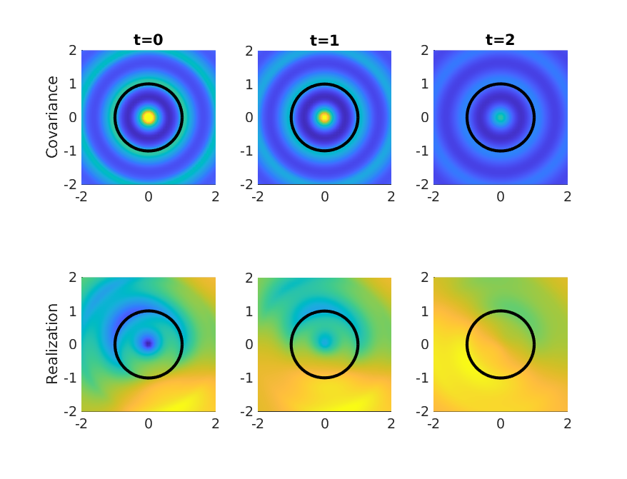
Figure 1: Top: worked example extending covariance (14) to $\mathbb{R}^{2}\times[0,\infty)$ via turning bands operator. Bottom: a realization of a Gaussian random field having this extended covariance at three consecutive time instants

Figure 1 shows the result for $d=2$ by numerically calculating the turning bands operator and simulating the corresponding Gaussian random field. The top panels plot the entire isotropic covariance function extended to the unit disc/plane via the turning bands operator, at three different time lags ($t=0,1,2$). The bottom three panels are a single realization of a Gaussian Random field (in $\mathbb{R}^{2}\times[0,\infty)$) plotted in the square $[-2,2]^{2}$ at three consecutive time instants $(0,1,2)$. The integration was computed in MATLAB R2019b using the adaptive quadrature of Shampine, (2008), and the realization of the Gaussian random field was computed using the covariance matrix decomposition method (Davis,, 1987), following an implementation of Wang and Constantine, (2012). The unit circle is drawn in black. The code to reproduce these results is shared at https://github.com/sffeng/extension.

References

- Berg and Porcu, (2017) Berg, C. and Porcu, E. (2017). From Schoenberg Coefficients to Schoenberg Functions. Constructive Approximation, 45:217–241.
- Calderon and Pepinsky, (1952) Calderon, A. and Pepinsky, R. (1952). On the phases of fourier coefficients for positive real periodic functions. Computing Methods and the Phase Problem in X-Ray Crystal Analysis, published by The X-Ray Crystal Analysis Laboratory, Department of Physics, The Pennsylvania State College, pages 339–348.
- Cambanis et al., (1983) Cambanis, S., Keener, R., and Simons, G. (1983). On -symmetric multivariate distributions. Journal of Multivariate Analysis, 13(2):213–233.
- Carathéodory, (1907) Carathéodory, C. (1907). Über den variabilitätsbereich der koeffizienten von potenzreihen, die gegebene werte nicht annehmen. Mathematische Annalen, 64(1):95–115.
- Crum, (1956) Crum, M. (1956). On positive-definite functions. Proceedings of the London Mathematical Society, 3(4):548–560.
- Daley and Porcu, (2013) Daley, D. J. and Porcu, E. (2013). Dimension Walks and Schoenberg Spectral Measures. Proc. Amer. Math. Society, 141:1813–1824.
- Davis, (1987) Davis, M. W. (1987). Production of conditional simulations via the LU triangular decomposition of the covariance matrix. Mathematical Geology, 19(2):91–98.
- Eaton, (1981) Eaton, M. L. (1981). On the projections of isotropic distributions. The Annals of Statistics, pages 391–400.
- Emery and Lantuéjoul, (2006) Emery, X. and Lantuéjoul, C. (2006). TBSIM: A computer program for conditional simulation of three-dimensional Gaussian random fields via the turning bands method. Computers Geosciences, 32(10):1615–1628.
- Emery and Porcu, (2019) Emery, X. and Porcu, E. (2019). Spectral simulation of multivariate isotropic Gaussian random fields on the sphere. Stochastic Environmental Research Risk Assessment, To Appear.
- Ern et al., (2018) Ern, M., Trinh, Q. T., Preusse1, P., Gille, J. C., Mlynczak, M. G., Russell, J. M., and Riese, M. (2018). GRACILE: a comprehensive climatology of atmospheric gravity wave parameters based on satellite limb soundings. Earth System Science Data, 10:857–892.
- Finlay, (2020) Finlay, C. C. (2020). Models of the main geomagnetic field based on multi-satellite magnetic data and gradients - Techniques and latest results from the Swarm missions. In M., D. and H., L., editors, Ionospheric Multi-Spacecraft Analysis Tools, pages 255–284. Springer, Cham: Switzerland.
- Gillet et al., (2013) Gillet, N., Jault, D., Finlay, C., and Olsen, N. (2013). Stochastic modeling of the Earth’s magnetic field: Inversion for covariances over the observatory era. Geochemistry, Geophysics, Geosystems, 14:766–786.
- Gneiting, (1999) Gneiting, T. (1999). Isotropic correlation functions on -dimensional balls. Advances in Applied Probability, 31(3):625–631.