The Nature of Reactive and Non-reactive Trajectories for a Three Dimensional Caldera Potential Energy Surface

Abstract

We used for the first time the method of periodic orbit dividing surfaces in a non-integrable Hamiltonian system with three degrees of freedom. We have studied the structure of these four dimensional objects in the five dimensional phase space. This method enabled us to detect the reactive and non-reactive trajectories in a three dimensional Caldera potential energy surface. We distinguished four distinct types of trajectory behavior. Two of the types of trajectories could only occur in a three dimensional Caldera potential energy surface and not in a two dimensional surface, and we have shown that this is a result of homoclinic intersections. These homoclinic intersections were analyzed with the method of Lagrangian descriptors. Finally, we were able to detect and describe the phenomenon of dynamical matching in the three dimensional Caldera potential energy surface, which is an important mechanism for understanding the reaction dynamics of organic molecules.

Keywords: Periodic orbit dividing surfaces, Caldera Potential, Dynamical matching, Chemical reaction dynamics.

I Introduction

Dynamical matching, originally observed by Carpenter [1, 2] , is an interesting phenomenon that is playing an increasingly important role for understanding the reactions of organic molecules, such as, the vinylcyclopropane-cyclopentene rearrangement [3, 4], the stereomutation of cyclopropane [5], the degenerate rearrangement of bicyclo[3.1.0]hex-2-ene [6, 7] or that of 5-methylenebicyclo[2.1.0]pentane [8].

Carpenter observed that the dynamical matching mechanism could be described by a two dimensional potential energy surface (PES) that resembles the collapsed region of an erupted volcano, to which the name ‘’caldera” was given in [9]. In particular, the caldera PES originally described by Carpenter has one minimum at the center and is surrounded by four index-1 saddles that control the entrance into and exit from the caldera region. Two of these index-1 saddles have low values of energy and the other two have high energy values, with respect to each other. The lower index-1 saddles correspond to the formation of the chemical products and the two higher index-1 saddles correspond to the reactants.

Trajectory behavior in this two dimensional (2D) Caldera PES has been extensively studied in recent years, see [10, 11, 12, 13, 14, 15]. A crucial requirement of these studies is to obtain collections of initial conditions corresponding to trajectories whose past and future behavior can be monitored in terms of the topographical features of the Caldera PES. For the associated two degree-of-freedom Hamiltonian systems this is accomplished with the method of periodic orbit dividing surfaces ([16, 17, 18, 19, 20, 21]. The dividing surfaces obtained from this method have one less dimension than the energy surface and are constructed from a periodic orbit. They satisfy the no-recrossing property (see for example [22]). If we consider trajectories that are initiated on the dividing surfaces of the unstable periodic orbits associated with the higher energy index-1 saddles we have two cases for the trajectory behavior(see [11, 12, 13, 14]):

1. In the first case, the trajectories that are initiated on the dividing surfaces of the unstable periodic orbits of the higher energy index-1 saddles go straight across the caldera and exit through the region of the opposite lower energy saddle. This trajectory behavior is what is referred to as dynamical matching. Understanding this behavior is very important for the caldera-type chemical reactions since 100$\%$ of the trajectories entering the Caldera from a region of one of the higher energy index-1 saddles exit through the region of one index-1 saddle, instead of $50\%$ crossing each of the lower energy index-1 saddles which is the prediction from statistical theories (see more details in the introduction of [10] and [2, 1]). We have previously shown that this behavior always occurs in 2D symmetric caldera potential energy surfaces because of the non-existence of intersections between the unstable invariant manifolds of the unstable periodic orbits of the higher index-1 saddles with the stable invariant manifolds of the unstable periodic orbits of the central area of the Caldera (see [11, 13]). If we break the symmetry, we can observe the trajectory behavior of the second case.

2. In the second case, the trajectories that start from the region of the higher energy index-1 saddles enter the caldera and may become trapped for a period of time before they exit from one of the regions of any of the four index-1 saddles. This is because the trajectories that have initial conditions on the dividing surfaces of the unstable periodic orbits of the higher energy index-1 saddles are trapped in the lobes between the unstable invariant manifolds of the unstable periodic orbits of the higher energy index-1 saddles and the stable invariant manifolds of unstable periodic orbits that exist in the central area of the Caldera (see [13, 12]). This case happens when we stretched the potential in the horizontal direction (see [12, 13, 14] or after a bifurcation of critical points ([23, 24] (in which we have a transition from a Caldera potential energy surface from one central minimum and four index-1 saddles to a Caldera with three index-1 saddles).

In this paper we develop a 3D model of the Caldera PES. This 3D extension of the 2D caldera potential energy surface is obtained by coupling a harmonic oscillator to one of the configuration space coordinates of the 2D Caldera PES. Hence, one can view this as a simple model of the 2D Caldera PES in a bath (with only a single bath mode).

We construct a 3D model of the Caldera PES and analyze the trajectory behavior. However, the passage to 3 dimensions brings significant new difficulties when attempting a similar analysis as the 2D case. In particular, the classical 2 DoF construction of periodic orbit dividing surfaces ([16],[20]) fails. The reason is using this approach the periodic orbits (1 dimensional objects) does not result in a 4 dimensional dividing surfaces in the 5 dimensional energy surface, which is what is required for a 3 DoF system.

The construction of dividing surfaces in Hamiltonian systems with three, and more, degrees of freedom has been accomplished with the use of a normally hyperbolic invariant manifold -NHIM ([25],[26],[27],[28][29]). But the computation of this object is difficult and limited in many cases and it requires extensive numerical calculations. Recently, we have developed a method that generalizes the periodic orbit dividing surface construction in Hamiltonian systems with three or more degrees of freedom ([30],[31]) that does not require the computation of a NHIM. In this paper we show how our construction of periodic orbit dividing surfaces can be applied in 3D for the analysis of dynamical matching.

This paper is outlined as follows. In Section II we describe our model of a 3D Caldera PES. The results are described in Section III. In particular, in Section III.1 we describe the construction of the 3D periodic orbit dividing surface and in Section III.2 we describe our analysis of trajectories that enter the Caldera. In Section IV we describe our conclusions.

II Model

The 3D potential energy surface (PES) for our model is constructed from a familiar 2D Caldera potential energy surface (that is symmetric with respect to the $y$-axis) and a harmonic oscillator in the $z$-direction that is coupled with the symmetry axis ($y$-axis) of the 2D Caldera PES. This can be viewed as a 2D Caldera coupled to a bath, where the bath has a single mode.

The 2D caldera PES that we used for our potential (see [10]) has the form:

$$V_{c}(x,y) =c_{1}r^{2}+c_{2}y-c_{3}r^{4}\cos(4\theta)$$ (1)

$$=c_{1}(x^{2}+y^{2})+c_{2}y-c_{3}(x^{4}+y^{4}-6x^{2}y^{2}),$$

where $(x,y)$ are Cartesian coordinates, $(r,\theta)$ are the standard polar coordinates, and $c_{1},c_{2},c_{3}$ are parameters. We used the same values for the parameters as in [10],[11],[12], [13] and [14], i.e. $c_{1}=5,c_{2}=3,c_{3}=-0.3$.

The 3D PES of our system, the 2D caldera potential plus a coupled harmonic oscillator in the $z$-direction, has the form:

$$V(x,y,z) =V_{c}(x,y)+c_{4}z^{2}+c_{5}yz^{2},$$ (2)

Where $c_{4}z^{2}$ and $c_{5}yz^{2}$ represents the harmonic oscillator and the coupling term, with $c_{4}=0.2$ and $c_{5}=0.03$. For a geometrical representation of this potential we show the 3D contours of this potentials in Fig. 1 or the contours of particular slices of this potential in Fig. 2. We see that this potential has the same topography in the $(x,y)$ space as that of the 2D Caldera, as can be seen from panels C and D of Fig. 2. We observe that the potential walls that are around the caldera in the $(x,y)$ subspace of the configuration space continue into the $z$-direction (Fig. 1 and panel A of Fig. 2). Furthermore, the topography of the potential for different slices in the $z$-direction is similar to that of the potential on the plane $z=0$ (that is equivalent to the potential of the 2D caldera).

The 3 degree-of-freedom (DoF) Hamiltonian is given by:

$$H(x,y,z,p_{x},p_{y},p_{z})=\frac{p_{x}^{2}}{2m}+\frac{p_{y}^{2}}{2m}+\frac{p_{z}^{2}}{2m}+V(x,y,z),$$ (3)

where $(x,y,z)$ are Cartesian coordinates and $p_{x}$, $p_{y}$, $p_{z}$ denote the momentum of the particle in $x-$, $y-$ and $z-$ direction respectively. We consider $m$ to be a constant equal to $1$. The Hamiltonian equations of motion are therefore:

$$\dot{x}=\frac{\partial H}{\partial p_{x}}=\frac{p_{x}}{m}$$ (4)

$$\dot{y}=\frac{\partial H}{\partial p_{y}}=\frac{p_{y}}{m}$$

$$\dot{y}=\frac{\partial H}{\partial p_{z}}=\frac{p_{z}}{m}$$

$$\dot{p_{x}}=-\frac{\partial V}{\partial x}(x,y,z)=-(2c_{1}x-4c_{3}x^{3}+12c_{3}xy^{2})$$

$$\dot{p_{y}}=-\frac{\partial V}{\partial y}(x,y,z)=-(2c_{1}y-4c_{3}y^{3}+12c_{3}x^{2}y+c_{2}+c_{5}z^{2})$$

$$\dot{p_{z}}=-\frac{\partial V}{\partial y}(x,y,z)=-(2c_{4}z+2c_{5}yz)$$

The 2D Caldera as we described in the introduction has one central minimum surrounded by 4 index-1 saddles. The 3D Caldera has the same equilibrium points (with $z=0$ for every equilibrium point). We give the position and the value of energy of the equilibrium points of the 3D Caldera potential in table I (for the set of the parameters $c_{1},c_{2},c_{3},c_{4}$ and $c_{5}$ that we used in our paper).

Table 1: Stationary points of the Caldera potential for $c_{1}=5,c_{2}=3$ $c_{3}=-0.3,c_{4}=0.2$ and $c_{5}=0.03$ ("RH" and "LH" are the abbreviations for right hand and left hand respectively)

Critical point	x	y	z	E
Central minimum	0.000	-0.297	0	-0.448
Upper LH saddle	-2.149	2.0778	0	27.0123
Upper RH saddle	2.149	2.0778	0	27.0123
Lower LH saddle	-1.923	-2.003	0	14.767
Lower RH saddle	1.923	-2.003	0	14.767

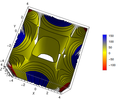
Figure 1: The contours of the 3D caldera potential in the $(x,y,z)$ space (where the color represents the value of the potential energy).

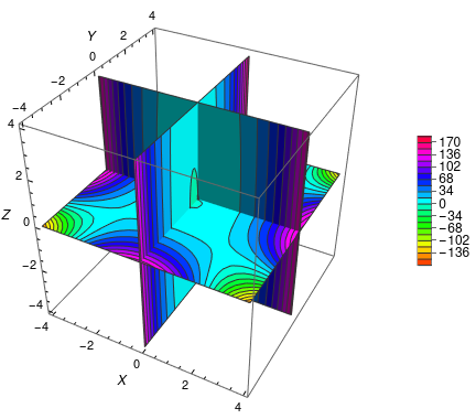
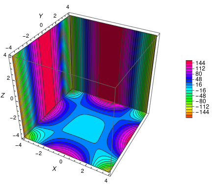
A) B)
C) D)

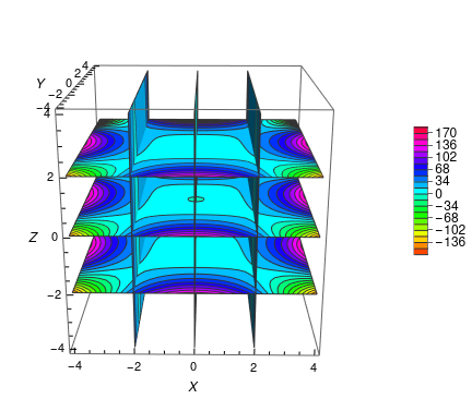
Figure 2: The slices of the contours of the 3D caldera potential in the $(x,y,z)$ space. A) The slices for $x=0$ and $y=0$. B) The slices for $z=-2$, $z=0$ and $z=2$. C) The slices for $x=-4$ and $y=4$. D) The slices for $z=-2$, $z=0$, $z=2$, $x=-2$, $x=0$ and $x=-2$.

III Results

In this section we will analyze the structure of the periodic orbit dividing surfaces that correspond to the unstable periodic orbits of the upper right index-1 saddle (we will have similar results for the periodic orbit dividing surfaces that correspond to the other index-1 saddles as a result of the symmetry of the potential) in the energy surface (see subsection III.1). Then we will present our results about the behavior of the trajectories that have initial conditions on these periodic orbit dividing surfaces and show how the periodic orbit dividing surfaces can detect the dynamical matching in a 3D Caldera-type system (see subsection III.2).

III.1 The construction and the structure of the periodic orbit dividing surfaces

In this subsection we describe the computation and the structure of the periodic orbit dividing surfaces for a non-integrable Hamiltonian system with three degrees-of-freedom. For this purpose we use our algorithm that we developed in previous papers (see [30, 31]). We will use the first algorithm of the construction of periodic orbit dividing surfaces that we proposed recently in [30]. We will apply this method for a fixed value of energy ($E=28$) above the higher index-1 saddle.

According to this algorithm we first compute one periodic orbit of the Lyapunov family of periodic orbits associated with the right higher index-1 saddle for a fixed value of energy ($E=28$). Then we follow the steps described below.

1. We check if the periodic orbit is a closed curve in one of the 2D projections of the configuration space. This is crucial for choosing which version of the algorithm of the construction of dividing surface is appropriate for our system (see [30]). In Fig. 3 we observe that the periodic orbit is not a closed curve in any 2D projection of the configuration space and this means that the second version of the algorithm in [30] is not valid.

2. Therefore we need to check if the first version of the algorithm is appropriate in our case. For this reason, we inspect if the periodic orbit is a closed curve in any of the 2D projections of the phase space. In Fig. 3 we see that this is true and this means that the first version of the algorithm is valid. The periodic orbit is represented by a closed curve in the $(y,p_{y})$ subspace of the phase space.

3. We construct a torus that is produced from the Cartesian product of a circle in the $(x,y)$ plane with the projection of the periodic orbit in the $(y,p_{y})$ subspace of the phase space. This Cartesian product gives us a two-dimensional torus in the $(x,y,p_{y})$ space. The radius of the circle, denoted $r$, is fixed at $r=0.25$.

4. We construct a torus that is produced from the Cartesian product of a circle in the $(y,z)$ plane with the torus that was constructed in the previous step. The result of this product is a three-dimensional torus in the $(x,y,z,p_{y})$ space. The radius of the circle is fixed at $r=0.25$.

5. We find for every point of the torus that was constructed in the previous step the maximum and minimum value of the momentum $p_{x}$. After this we take values for $p_{x_{i}}$ $i=1,...n$ in the interval $[p_{x}min,p_{x}max]$. In this way, we add a segment at the torus of the previous step increasing its dimensionality from three to four. In this step we used $n=5$ for our computations.

6. For every point of the four-dimensional torus that was constructed in the previous step we find the last momentum $p_{z}$ from the Hamiltonian.

The structure of the periodic orbit dividing surfaces that were constructed from the algorithm is depicted in Figs. 4, 5 and 6. In order to see better the structure of these objects we increase the number of values of $p_{x}$ (from $n=5$ to $n=21$) in the fifth step of the algorithm. The periodic orbit dividing surface is a 4-dimensional torus in the 5-dimensional energy surface $(x,y,z,p_{x},p_{y})$ (see [30]). This structure is represented by toroidal structures in the 3D projections $(x,y,z),(x,y,p_{y}),(x,z,p_{y})$ and $(x,p_{x},p_{y})$ of the phase space that are similar to the structure of Fig. 4. Furthermore, the periodic orbit dividing surface has the morphology of a hyperboloid in the 3D projections $(x,y,p_{x})$ and $(y,p_{x},p_{y})$ of the phase space (see for example the 3D projection $(x,y,p_{x})$ in panel A of Fig. 5). The hyperbolic behavior of this structure can be seen better in some of the 2D projections of this object (see for example the projection $(x,y)$ in the panel B of Fig. 5). In the other 3D projections, the periodic orbit dividing surface has a boxy structure (see the boxy structure in Fig. 6).

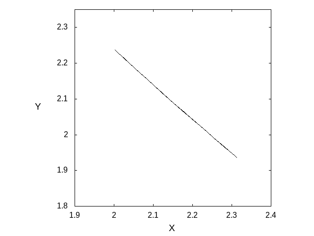
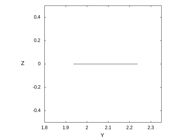
A) B)
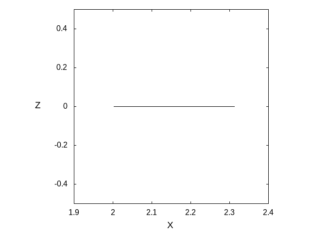
C) D)

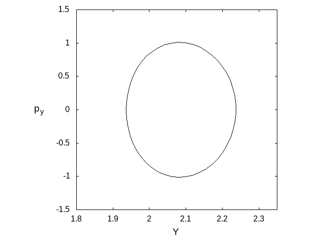
Figure 3: The ($(x,y),(x,z),(y,z)$ and $(y,p_{y}$ projections of the periodic orbit of the Lyapunov family of the right higher index-1 saddle for $E=28$.

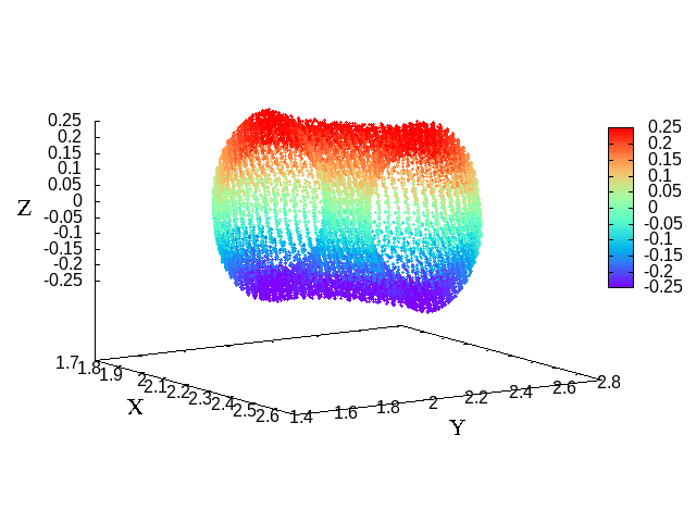
Figure 4: The periodic orbit dividing surface for $E=28$ in the $(x,y,z)$ subspace of the phase space. The color indicates the third dimension.

A)
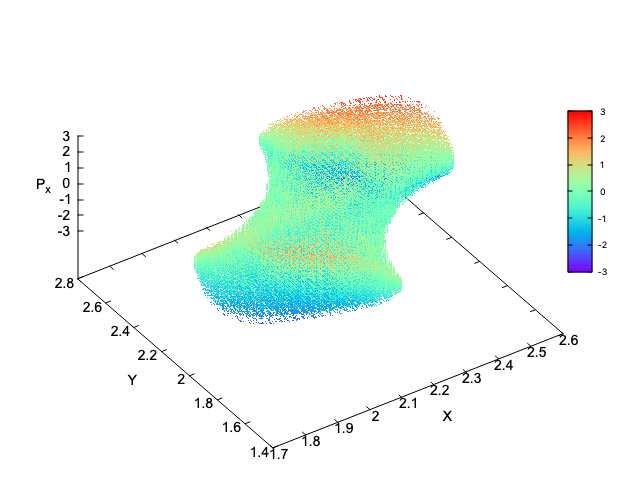
B)

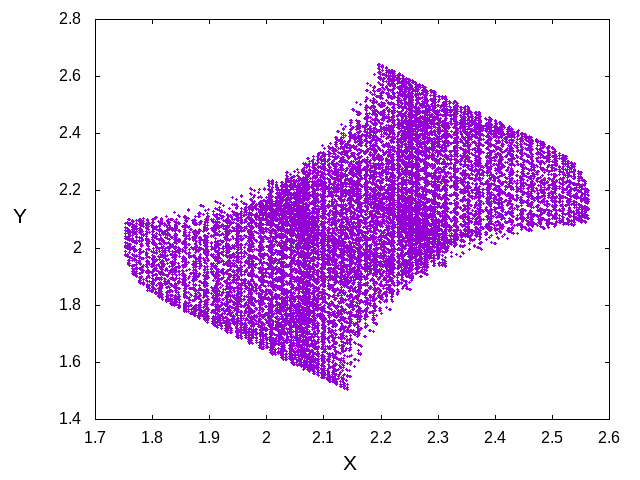
Figure 5: Panel A:The periodic orbit dividing surface for $E=28$ in the $(x,y,p_{x})$ subspace of the phase space. The color indicates the third dimension. Panel B: The 2D projection $(x,y)$ of the periodic orbit dividing surface for $E=28$.

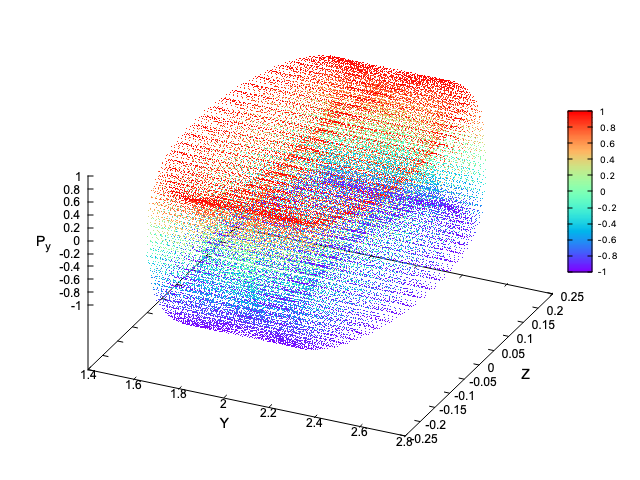
Figure 6: The periodic orbit dividing surface for $E=28$ in the $(y,z,p_{y})$ subspace of the phase space.The color indicates the third dimension.

III.2 Dynamical Matching

In this subsection we study the behavior of the trajectories that have initial conditions on the periodic orbit dividing surface associated with the upper right index-1 saddle for $E=28$. We construct the periodic orbit dividing surface using the algorithm described in the previous subsection (for $r=0.25,n=5$ that corresponds to 21.178 initial conditions). Then we integrated the initial conditions on this periodic orbit dividing surface forward and backward in time for 7 time units (this time interval is enough for all trajectories to exit from the caldera). We classified the resulting trajectories into reactive and non-reactive trajectories and labelled the initial conditions on the dividing surface accordingly. The reactive trajectories have a direction towards the center of the caldera forward in time. On the contrary, the non-reactive trajectories become unbounded forward in time. We encountered four types of trajectory behavior:

1. First type: For this type, the trajectories (7176 trajectories $\approx 33.88\%$ of the initial trajectories on the dividing surface), that start from the periodic orbit dividing surface associated with the right upper index-1 saddle, go straight across the caldera (see Fig. 7) and exit through the region of the opposite index-1 saddle. This happens if we integrate the initial conditions on the dividing surface forward and backward. This means that the trajectories go initially to the direction of the reaction (that is the region of the lower index-1 saddles) and exit through only from the region of the opposite lower index-1 saddle. These trajectories belong to the reactive part of this periodic orbit dividing surface and correspond to $\approx 33.88\%$ of the initial trajectories on the dividing surface.

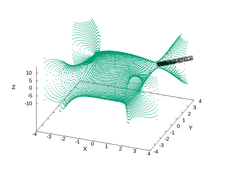
Figure 8: Panel A: The evolution of the trajectories (with red forward in time), that have initial conditions on the dividing surface associated with the periodic orbits of the upper right index-1 saddle and they move in the opposite direction of the reaction, in the configuration space $(x,y,z)$. Panel B: The evolution of the trajectories (with black backward in time), that have initial conditions on the dividing surface associated with the periodic orbits of the upper right index-1 saddle and they move in the opposite direction of the reaction, in the configuration space $(x,y,z)$. In all panels, we depict the zero velocity surface using green color.

2. Second type: For this type, if we integrate (forward or backward) the initial conditions on the periodic orbit dividing surface associated with the right upper index-1 saddle, the resulting trajectories go directly to infinity (see Fig. 8). These trajectories (7312 trajectories, $\approx 34.53\%$ of the initial trajectories on the dividing surface) belong to the non-reactive part of this periodic orbit dividing surface.

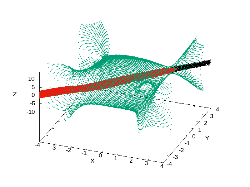
Figure 9: The evolution of the trajectories (with red forward in time), that have initial conditions on the dividing surface associated with the periodic orbits of the upper right index-1 saddle and they move in the direction of the reaction, in the configuration space $(x,y,z)$. The evolution of the trajectories (with black backward in time), that have initial conditions on the dividing surface associated with the periodic orbits of the upper right index-1 saddle and they move in the opposite direction of the reaction, in the configuration space $(x,y,z)$. In all panels, we depict the zero velocity surface using a green color.

3. Third type: For this type, the trajectories (that start from the periodic orbit dividing surface associated with the right upper index-1 saddle) go straight across the caldera and they exit through the opposite lower saddle under forward integration (see Fig. 9). These trajectories go directly to infinity backward in time (see Fig. 9). This means that these trajectories (3314 trajectories $\approx 15.65\%$ of the initial trajectories on the dividing surface) belong to the reactive part of this periodic orbit dividing surface.

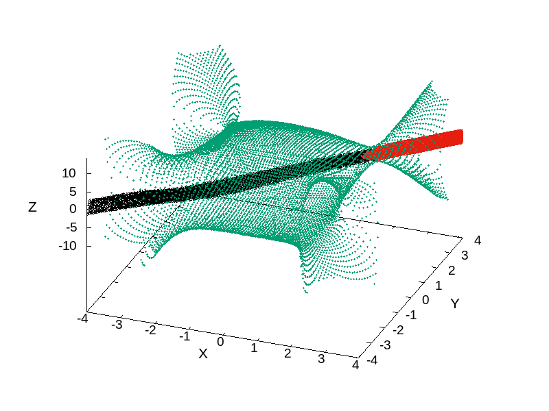
Figure 10: The evolution of the trajectories (with red forward in time), that have initial conditions on the dividing surface associated with the periodic orbits of the upper right index-1 saddle and they move in the opposite direction of the reaction, in the configuration space $(x,y,z)$. The evolution of the trajectories (with black backward in time), that have initial conditions on the dividing surface associated with the periodic orbits of the upper right index-1 saddle and they move in the direction of the reaction, in the configuration space $(x,y,z)$. In all panels, we depict the zero velocity surface using a green color.

4. fourth type: For this type, the trajectories (with initial conditions on the periodic orbit dividing surface associated with the right upper index-1 saddle) go directly to the infinity forward in time and go straight across the caldera, and exit through the lower opposite saddle backward in time (see Fig. 10). In this type, the trajectories (3376 trajectories $\approx 15.94\%$ of the initial trajectories on the dividing surface) do not belong to the reactive part of the dividing surface because they move in the opposite direction forward in time.

We observe that the first and third types of trajectories correspond to the reactive part ($\approx 49.53\%$ of the initial conditions on the dividing surface) of the dividing surface and the second and fourth types of trajectories correspond to the non-reactive part of the dividing surface. All types of the trajectory behavior of the reactive part correspond to the phenomenon of dynamical matching since for these types all trajectories exit through the opposite lower saddle forward in time.

Furthermore, we note that the first and second type of trajectory behavior includes trajectories that you can find only in the 3D caldera and not in the 2D caldera. This happens because in these cases the trajectories move in the same direction (in the direction of reaction or in the opposite direction) forward and backward in time, following different paths in the third dimension. These trajectories (Fig.11) form a horseshoe embedded in the 3D configuration space. The one branch of this horseshoe corresponds to the forward evolution in time and the other to the backward evolution in time. This explains why the trajectories move in the same direction forward and backward in time.

The trajectory behavior of Fig. 11 resembles the trajectory behavior that we encounter in lobes between homoclinic intersections. For example, if we had a trajectory in a lobe between homoclinic intersections of the stable and unstable manifold of the NHIM that is associated with the lower-left index-1 saddle, we would have the same trajectory behavior with that of the panel A of Fig. 11. Similarly, if we had a trajectory in a lobe between homoclinic intersections of the stable and unstable manifolds of the NHIM associated with the upper right index-1 saddle, we would have the same trajectory behavior as that of the panel B of Fig. 11. The Normally Hyperbolic Invariant Manifold -NHIM (see for example [29]) is a 3D geometrical object in the phase space of a Hamiltonian system with three degrees of freedom. The invariant manifolds of the NHIMs are 4-dimensional objects in the phase space of a Hamiltonian system with three degrees of freedom. The 2D slices of the invariant manifolds of NHIMs will be 1-dimensional objects and will be presented as lines or curves in these slices.

In order to check the hypothesis of the previous paragraph for the origin of the trajectory behavior that is shown in Fig. 11, we will use the method of Lagrangian descriptors (LDs) (see the books [15, 32] and the references therein). The method of Lagrangian descriptors (LDs) is a trajectory-based scalar diagnostic tool that can be used to probe 2D slices of the phase space. We have used this method for analyzing the 2D Caldera potential energy surface recently (see [13, 14] - the reader can find details in these references about the computation of LDs in a caldera-type potential). We will apply the same method in 2D slices of the phase space as we did for the 2D caldera potential energy surface (with the only difference that now we will integrate six equations of motion instead of four). In this paper we checked if the initial conditions of the trajectories of the first and second types trajectories belong in lobes between the stable and unstable invariant manifolds of NHIMs (that are computed using LDs). We present as an example the initial condition of the first type trajectory that is depicted in panel A of Fig. 11. This trajectory has as initial condition $x=2.120469667800,y=1.946617848594,z=0.237764129074,p_{x}=-0.526679066677,p_{y}=0.957219684607,p_{z}=0.912234902767$. We will compute the LDs in the 2D slice $(x,p_{x})$ space with $y=1.946617848594,z=0.237764129074,p_{z}=0.912234902767$ (computing $p_{y}$ from the Hamiltonian). We computed the LDs, using forward (for stable invariant manifolds) and backward (for unstable invariant manifolds) integration, in this slice (see the panels A and B of Fig.12). Then we restricted our analysis in a smaller area (see panels C and D of Fig. 12) in which we have the initial condition of the trajectory in panel A of Fig. 11. In order to visualize better the lobes between the intersections of the invariant manifolds of the NHIMs we extract the invariant manifolds from the gradient of LDs (see for details [32, 13]) and we plotted them together in Fig. 13. We observe that the initial condition of the trajectory of panel A of Fig.11 is in the lobe between the intersections of the stable and unstable invariant manifolds of a NHIM. As we can see in Fig. 11 this trajectory goes (forward and backward) to the region of the lower left index-1 saddle. This means that the lobe, where the initial condition of this trajectory is inside, is between the homoclinic intersections of the stable and unstable invariant manifolds of the NHIM associated with the lower left index-1 saddle. Similarly, we can find that all the initial conditions of the first and second type trajectories are inside the lobes of homoclinic intersections of the invariant manifolds of the NHIM associated with the lower left index-1 saddle and of the NHIM associated with the the upper right index-1 saddle, respectively.

A)
B)

Figure 7: Panel A: The evolution of the trajectories (with red forward in time), that have initial conditions on the dividing surface associated with the periodic orbits of the upper right index-1 saddle and they move in the direction of the reaction, in the configuration space $(x,y,z)$. Panel B: The evolution of the trajectories (with black backward in time), that have initial conditions on the dividing surface associated with the periodic orbits of the upper right index-1 saddle and they move in the direction of the reaction, in the configuration space $(x,y,z)$. In all panels, we depict the zero velocity surface using a green color.

A)
B)

A)
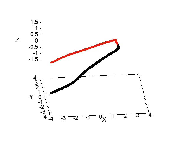
B)

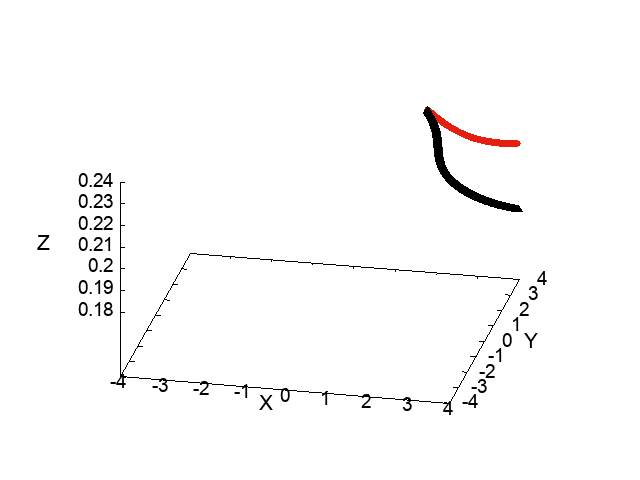
Figure 11: A) One first type trajectory (with red and black color in forward and backward in time respectively). B) One second type trajectory (with red and black color in forward and backward in time respectively).

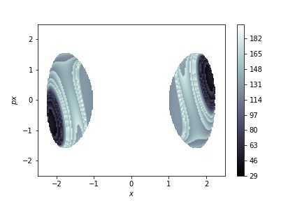
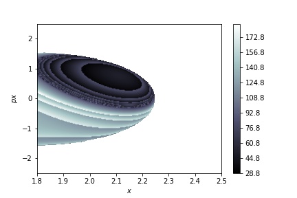
A) B)
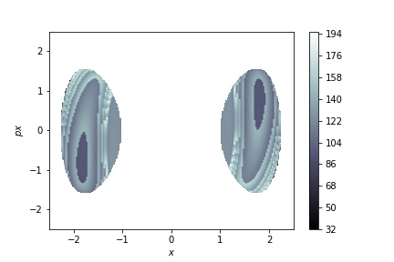
C) D)

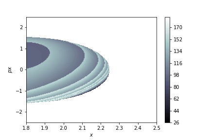
Figure 12: Computation of variable-time LDs in the 2D slide $y=1.946617848594,z=0.237764129074,p_{z}=0.912234902767$ using $\tau=2$ and p = 1/2. A) Forward integration LDs; B) Backward integration LDs; C) Forward integration for the interval $1.8<x<2.5$. D) Backward integration for the interval $1.8<x<2.5$.

A)

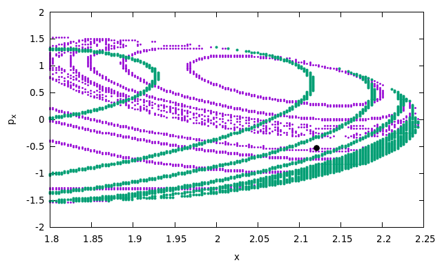
Figure 13: The stable (violet) and unstable (green) invariant manifolds extracted (in the 2D slice $y=1.946617848594,z=0.237764129074,p_{z}=0.912234902767$) from the gradient of the Lagrangian descriptors for the interval $1.8<x<2.5$. We depict using black color the initial condition of a first type trajectory that is shown in Fig. 11.

IV conclusions

In this paper, we computed the periodic orbit dividing surfaces in a 3D non-integrable Hamiltonian system. We studied the structure of these dividing surfaces and found that they have a Hyperboloid or a toroidal structure that is represented as a toroidal structure or a Hyperboloid or a box structure in 3D projections of the phase space. This result is in agreement with the structure of the same surfaces that are studied in the case of an integrable Hamiltonian system with three degrees of freedom (see [30]). The only difference is that the periodic orbit dividing surfaces are not so smooth as in the integrable case of a Hamiltonian system with three degrees of freedom.

Using the periodic orbit dividing surfaces we distinguished the reactive and non-reactive parts of a 3D Caldera potential energy surface. We found four types of trajectory behaviors associated with the upper index-1 saddles (trajectories that start from the periodic orbit dividing surfaces associated with the unstable periodic orbits of the upper index-1 saddles). The first and third types correspond to the reactive part and the second and fourth types to the non-reactive part. The reactive part is about $49.53\%$ of the trajectories that start from the periodic orbit dividing surface associated with the upper index-1 saddles. All trajectories of the reactive part go straight across the caldera and they exit through the region of the opposite lower index-1 saddle. This is the phenomenon of dynamical matching, that was detected for the first time in a 3D potential energy surface. The first and second types of trajectories are a consequence of homoclinic intersections of the invariant manifolds of the NHIM associated with the lower index-1 saddles and the opposite upper index-1 saddles, respectively.

References

- Carpenter [1995] B. Carpenter, J. Am. Chem. Soc. 117, 6336 (1995).
- Carpenter [1985] B. K. Carpenter, Trajectories through an intermediate at a fourfold branch point. implications for the stereochemistry of biradical reactions, Journal of the American Chemical Society 107, 5730 (1985).
- Baldwin [2003] J. Baldwin, Thermal rearrangements of vinylcyclopropanes to cyclopentenes, Chemical reviews 103, 1197 (2003).
- Goldschmidt and Crammer [1988] Z. Goldschmidt and B. Crammer, Vinylcyclopropane rearrangements, Chem. Soc. Rev 17, 229 (1988).
- Doubleday et al. [1997] C. Doubleday, K. Bolton, and W. Hase, Direct dynamics study of the stereomutation of cyclopropane, Journal of the American Chemical Society 119, 5251 (1997).
- Doubleday et al. [1999] C. Doubleday, M. Nendel, K. Houk, D. Thweatt, and M. Page, Direct dynamics quasiclassical trajectory study of the stereochemistry of the vinylcyclopropane - cyclopentene rearrangement, Journal of the American Chemical Society 121, 4720 (1999).
- Doubleday et al. [2006] C. Doubleday, C. Suhrada, and K. Houk, Dynamics of the degenerate rearrangement of bicyclo[3.1.0]hex-2-ene, Journal of the American Chemical Society 128, 90 (2006).
- Reyes et al. [2002] M. Reyes, E. Lobkovsky, and B. Carpenter, Interplay of orbital symmetry and nonstatistical dynamics in the thermal rearrangements of bicyclo[n.1.0]polyenes, J Am Chem Soc 124, 641 (2002).
- Doering et al. [2002] W. v. E. Doering, X. Cheng, K. Lee, and Z. Lin, Fate of the intermediate diradicals in the caldera:_ stereochemistry of thermal stereomutations, (2 + 2) cycloreversions, and (2 + 4) ring-enlargements of cis- and trans- 1-cyano-2-(e_and_z)-propenyl-cis-3,4-dideuteriocyclobutanes, Journal of the American Chemical Society 124, 11642 (2002).
- Collins et al. [2014] P. Collins, Z. Kramer, B. Carpenter, G. Ezra, and S. Wiggins, Nonstatistical dynamics on the caldera, Journal of Chemical Physics 141 (2014).
- Katsanikas and Wiggins [2018] M. Katsanikas and S. Wiggins, Phase space structure and transport in a caldera potential energy surface, International Journal of Bifurcation and Chaos 28, 1830042 (2018).
- Katsanikas and Wiggins [2019] M. Katsanikas and S. Wiggins, Phase space analysis of the nonexistence of dynamical matching in a stretched caldera potential energy surface, International Journal of Bifurcation and Chaos 29, 1950057 (2019).
- Katsanikas et al. [2020a] M. Katsanikas, V. J. García-Garrido, and S. Wiggins, The dynamical matching mechanism in phase space for caldera-type potential energy surfaces, Chemical Physics Letters 743, 137199 (2020a).
- Katsanikas et al. [2020b] M. Katsanikas, V. J. García-Garrido, and S. Wiggins, Detection of dynamical matching in a caldera hamiltonian system using lagrangian descriptors, Int. J. Bifurcation Chaos 30, 2030026 (2020b).
- Agaoglou et al. [2019] M. Agaoglou, B. Aguilar-Sanjuan, V. J. García-Garrido, R. García-Meseguer, F. González-Montoya, M. Katsanikas, V. Krajňák, S. Naik, and S. Wiggins, Chemical Reactions: A Journey into Phase Space (Bristol, UK, Zenodo, 2019).
- Pechukas and McLafferty [1973] P. Pechukas and F. J. McLafferty, On transition-state theory and the classical mechanics of collinear collisions, The Journal of Chemical Physics 58, 1622 (1973).
- Pechukas and Pollak [1977] P. Pechukas and E. Pollak, Trapped trajectories at the boundary of reactivity bands in molecular collisions, The Journal of Chemical Physics 67, 5976 (1977).
- Pechukas and Pollak [1979] P. Pechukas and E. Pollak, Classical transition state theory is exact if the transition state is unique, The Journal of Chemical Physics 71, 2062 (1979).
- Pechukas [1981] P. Pechukas, Transition state theory, Annual Review of Physical Chemistry 32, 159 (1981).
- Pollak and Pechukas [1978] E. Pollak and P. Pechukas, Transition states, trapped trajectories, and classical bound states embedded in the continuum, The Journal of Chemical Physics 69, 1218 (1978).
- Pollak [1985] E. Pollak, Periodic orbits and the theory of reactive scattering, Theory of Chemical Reaction Dynamics 3, 123 (1985).
- Ezra and Wiggins [2018] G. S. Ezra and S. Wiggins, Sampling phase space dividing surfaces constructed from normally hyperbolic invariant manifolds (nhims), The Journal of Physical Chemistry A 122, 8354 (2018).
- Geng et al. [2021a] Y. Geng, M. Katsanikas, M. Agaoglou, and S. Wiggins, The influence of a pitchfork bifurcation of the critical points of a symmetric caldera potential energy surface on dynamical matching, Chemical Physics Letters 768, 138397 (2021a).
- Geng et al. [2021b] Y. Geng, M. Katsanikas, M. Agaoglou, and S. Wiggins, The bifurcations of the critical points and the role of the depth in a symmetric caldera potential energy surface, Int. J. Bifurcation Chaos 31 (2021b).
- Wiggins [1994] S. Wiggins, Normally hyperbolic invariant manifolds in dynamical systems (springer verlag, 1994).
- Wiggins et al. [2001] S. Wiggins, L. Wiesenfeld, C. Jaffé, and T. Uzer, Impenetrable barriers in phase-space, Physical Review Letters 86, 5478 (2001).
- Komatsuzaki and Berry [2003] T. Komatsuzaki and R. S. Berry, Chemical reaction dynamics: Many-body chaos and regularity, Adv. Chem. Phys. , 79 (2003).
- Uzer et al. [2002] T. Uzer, C. Jaffé, J. Palacián, P. Yanguas, and S. Wiggins, The geometry of reaction dynamics, Nonlinearity 15, 957 (2002).
- Wiggins [2016] S. Wiggins, The role of normally hyperbolic invariant manifolds (nhims) in the context of the phase space setting for chemical reaction dynamics, Regular and Chaotic Dynamics 21, 621 (2016).
- Katsanikas and Wiggins [2021a] M. Katsanikas and S. Wiggins, The generalization of the periodic orbit dividing surface for Hamiltonian systems with three or more degrees of freedom in chemical reaction dynamics - I, International Journal of Bifurcation and Chaos 31, 2130028 (2021a).
- Katsanikas and Wiggins [2021b] M. Katsanikas and S. Wiggins, The generalization of the periodic orbit dividing surface for Hamiltonian systems with three or more degrees of freedom in chemical reaction dynamics - II, International Journal of Bifurcation and Chaos 31, 2150188 (2021b).
- Agaoglou et al. [2020] M. Agaoglou, B. Aguilar-Sanjuan, V. J. García-Garrido, F. González-Montoya, M. Katsanikas, V. Krajňák, S. Naik, and S. Wiggins, Lagrangian Descriptors: Discovery and Quantification of Phase Space Structure and Transport (zenodo: 10.5281/zenodo.3958985, 2020).