HiMODE: A Hybrid Monocular Omnidirectional Depth Estimation Model

Abstract

Monocular omnidirectional depth estimation is receiving considerable research attention due to its broad applications for sensing $360^{\circ}$ surroundings. Existing approaches in this field suffer from limitations in recovering small object details and data lost during the ground-truth depth map acquisition. In this paper, a novel monocular omnidirectional depth estimation model, namely HiMODE is proposed based on a hybrid CNN+Transformer (encoder-decoder) architecture whose modules are efficiently designed to mitigate distortion and computational cost, without performance degradation. Firstly, we design a feature pyramid network based on the HNet block to extract high-resolution features near the edges. The performance is further improved, benefiting from a self and cross attention layer and spatial/temporal patches in the Transformer encoder and decoder, respectively. Besides, a spatial residual block is employed to reduce the number of parameters. By jointly passing the deep features extracted from an input image at each backbone block, along with the raw depth maps predicted by the transformer encoder-decoder, through a context adjustment layer, our model can produce resulting depth maps with better visual quality than the ground-truth. Comprehensive ablation studies demonstrate the significance of each individual module. Extensive experiments conducted on three datasets; Stanford3D, Matterport3D, and SunCG, demonstrate that HiMODE can achieve state-of-the-art performance for $360^{\circ}$ monocular depth estimation.

1 Introduction

Depth estimation is a fundamental technique to facilitate 3D scene understanding from a single 2D image for real-world applications such as autonomous driving [23], virtual reality (VR) [2], robotics [22], 3D reconstruction [25], object detection [26], and augmented reality (AR) [21]. Earlier depth estimation techniques utilized the sensor-based or stereo vision-based approaches, with the passive stereo vision systems gaining more attention due to their comparatively better performance in many real-world scenarios. However, availability of standard multi-view stereo datasets is scarce due to deferring alignment and camera settings.

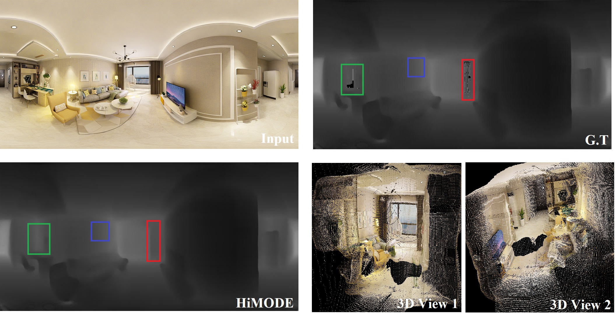
Figure 1: An example of a panorama image with its corresponding depth map and 3D structure generated by HiMODE. Our proposed hybrid CNN+Transformer model provides highly accurate depth map with fewer artifacts than even the ground-truth which contains many holes.

This limitation inspired researchers to divert their attention to monocular depth estimation (MDE) as a desirable alternative. Due to significant advances in GPUs and availability of large-scale 3D datasets, several deep learning-based MDE methods were reported in the literature with promising results [18, 14, 19]. The downside of these approaches is that the perspective images have limited FOV.

The emergence of modern $360^{\circ}$ cameras presented an appealing solution [40, 9]. Omnidirectional images provide $360^{\circ}$ FOV, formed by extending a 3D spherical construction to a 2D $360^{\circ}\times 180^{\circ}$ equirectangular map . Naive extension of MDE methods (e.g. FCRN [18]) to $360^{\circ}$ images may result in geometric distortion and image discontinuity, leading to sub-optimal results [44]. This motivates researchers to conduct further studies on omnidirectional MDE. Several approaches based on Convolutional Neural Networks (CNNs) have been proposed for omnidirectional depth estimation. Although these methods could successfully estimate the depth map around the equator, their performance declined sharply in regions with significant distortions (e.g., poles) due to their limited receptive field. Recently, Transformer-based methods [32] have been shown to surpass CNNs with their competitive performance in various vision tasks. However, due to the lack of inductive bias in Transformers, dealing with small-scale datasets is challenging [8]. Several researchers attempted to make the performance of the Transformers independent of data [31] but it is still an open problem. Although HoHoNet in [29] had a structure similar to Transformer attention, the approach in [41] was the first in directly applying the Transformers to the field of $360^{\circ}$ MDE. It achieved good performance when pre-trained on the large-scale dataset of traditional rectilinear images (RIs) and fine-tuned for panoramic images. However, its performance was inferior in case it was directly trained on the small datasets of panoramic images.

To address the above-mentioned challenges, we propose HiMODE, a novel hybrid CNN-Transformer framework that capitalizes on the strengths of CNN-based feature extractors and the power of Transformers for monocular omnidirectional depth estimation. Benefiting from combining both low-level and high-level feature maps extracted by the CNN-based backbone, along with the raw depth maps estimated by the Transformer encoder-decoder via a context adjustment layer, HiMODE not only performs competitively on the existing small-scale datasets, but can also accurately recover the surface depth data lost in the G.T depth maps. An example of a resulting depth map, with its corresponding 3D structure, is illustrated in Figure 1 to demonstrate the competitive performance and capabilities of HiMODE in dealing with distortion and artifacts. This competitive performance is accomplished via several mechanisms; i.e. a feature pyramid network in the design of CNN-based backbone, and a single block of encoder and decoder in the Transformer that comprises several modules - spatial and temporal patches (STP), spatial residual block (SRB), and self and cross attention (SCA) block, in place of the typical multi-head self-attention (MHSA) in encoder. More specifically, the key contributions of this paper include:

• A novel end-to-end hybrid architecture, that combines CNN and Transformer for monocular omnidirectional depth estimation, obtaining competitive performance even when trained on small-scale datasets.

• A novel depth-wise CNN-based backbone network that can extract high-resolution features near the edges to overcome distortion and artifact issues (at object boundaries), and refine the predicted raw depth maps with low- to high-level feature maps via context adjustment layer to obtain results even better than G.T.

• A novel single encoder-decoder Transformer designed with the SCA layer in place of the MHSA layer in the Transformer encoder for better encoding the parameters, and a STP layer along with the MHSA layer in the Transformer decoder to reduce the size of the training parameters while improving the depth map prediction.

• A spatial residual block (SRB) that is added after both the encoder and decoder, for training stabilization and performance improvement. The SRB allocates more channels to high-level patches in deeper levels and retains equivalent computation when resolution is reduced.

• Results of extensive experiments demonstrate that HiMODE can achieve state-of-the-art performance across three benchmarks datasets.

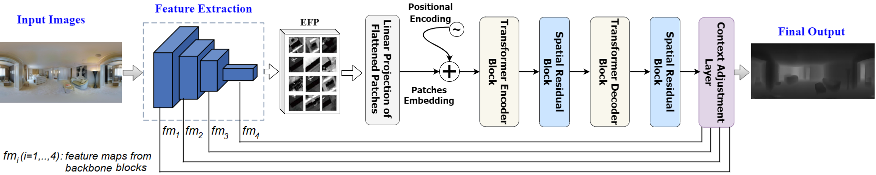
Figure 2: The proposed HiMODE architecture consists of a CNN-based feature extractor and a Transformer encoder-decoder.

2 Related Works

Monocular depth estimation based on equirectangular images (EIs) was first attempted in [30] and [44]. Tateno et al. [30] minimized the distortion based on CNNs and Zioulis et al. [44] proposed a pre-processing step including simplistic rectangular filtering. Later in [43], the $360^{\circ}$ view synthesis was investigated in a self-supervised manner. As the left and right sides of the EIs are adjacent in the panorama sphere format, Lai et al. [17] proposed a deep network with a boundary loss function to minimize the distortion effects. In [7], the details of depth were preserved by employing both perspective and $360^{\circ}$ cameras.

In the BiFuse [34] method, a two-branch neural network was proposed to use two projections of equirectangular and cube map for imitating both human eye visions of peripheral and foveal. In [29], Sun et al. proposed HoHoNet, a versatile framework for holistic understanding of indoor panorama images based on a combination of compression and self attention modules. These approaches achieved satisfactory performance for the indoor scenarios. To deal with outdoor scenes with wider FOV, Xu et al. [36] proposed a graph convolutional network (GCN) with a distortion factor in the adjacency matrix for real-time depth estimation.

Li et al [20] proposed a novel two-stage pipeline for omnidirectional depth estimation. In their method, the main input was a single panoramic image used in the first stage to generate one or more synthesized views. These synthesized images, along with the original $360^{\circ}$ image, were fed into a stereo matching network with a differentiable spherical warping layer to produce dense, high-quality depth. To evaluate the methods based on two important traits of boundary preservation and smoothness, an unbiased holistic benchmark, namely Pano3D, was proposed in [1]. Additionally, Pano3D evaluated the inter-dataset performance as well as the intra-dataset performance. In a very recent study in [41], a new $360^{\circ}$ MDE system was proposed by combining supervised and self-supervised learning. They applied a Vision Transformer (ViT) for the first time in this field and achieved competitive performance. In summary, existing approaches have shown improvement in depth estimation, but there exists an obvious need for performance precision and distortion minimization.

3 Proposed Network

The proposed HiMODE architecture, which comprises of a CNN-based feature extractor and a Transformer encoder-decoder, along with the linear projection (LP), positional encoding, spatial residual, and context adjustment modules, is presented in Figure 2. The details of each module are discussed in the following subsections.

3.1 Depth-wise CNN-based Backbone

Many CNNs, such as MobileNet, ResNet, etc., are used as the backbone for feature extraction. The extracted feature maps are mostly ten to a hundred times bigger than the model size in these backbones, particularly for high-level feature extraction operations, resulting in high computation cost and high dynamic RAM traffic. To diminish this high traffic, the size of the feature maps is minimized with lossy compression methods such as subsampling. Inspiring by this, we design a novel depth-wise separable CNN-based backbone with a feature pyramid network to decrease the size of the extracted feature maps without sacrificing the accuracy. It has an efficient structure for extracting high-resolution features near the edges.

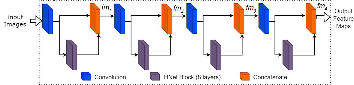
Figure 3: The detailed architecture of the proposed feature extractor formed by concatenation of convolution and HNet blocks.

As illustrated in Figure 3, the proposed backbone is composed of four single-layer convolution blocks, four HNet blocks (each block with eight layers), and four concatenation blocks for merging the feature maps generated from two former blocks. The HNet is a lightweight block extracted from HardNet [6] and formed by two main sub-blocks of dense harmonic and depth-wise convolution (as the high-level feature extraction module) to reduce the memory computation cost and to fuse the features (for compression). Differing from HardNet which has 68 layers, our backbone consists of only 40 layers with superior performance over the other pre-trained models.

3.2 Linear Projection and Positional Encoding

Generally, the input of a standard Transformer is required to be a 1D sequence of token embeddings. Hence, the extracted feature maps of $X\in\mathbb{R}^{H\times W\times C}$ from our backbone are first split into patches, i.e., extracted feature patches (EFP), with a fixed size of $p\times p$ ($p=8$). These patches are reshaped into a sequence of flattened 2D patches $X_{p}\in\mathbb{R}^{N\times(p^{2}C)}$ ($N=\frac{HW}{p^{2}}$ is the sequence length). These flattened patches are passed to a linear projection module to generate lower-dimensional linear embeddings with less computation cost. In the linear projection layer, each patch is first unrolled into a vector multiplied with a learnable embedding matrix to form the Patch Embeddings ($PE$), which are then concatenated with the Positional Embeddings ($PE^{\prime}$) to be fed into the Transformer.

Distinguishing the similarities and differences between the pixels in vast texture-less regions is a challenging issue which can be addressed by considering the relative location of information. Thus, we find the spatial information of the EFP using the positional encoding module. The adequate positional information of the patches is encoded for the irregular patch embedding. Consequently, the overall performance is enhanced as the EFP is equipped with spatial/positional information before being fed into the transformer encoder. Positional Embeddings ($PE^{\prime}$) are obtained via the positional encoding formulation as follows [32]:

$$PE^{\prime}_{(pos,2i)}=sin(pos/10000^{2i/D})$$ (1)

where $pos$ and $i$ are respectively the position of the patches and the dimensional position in the $D$-dimensional vector ($D=256$, is the dimension of the vector into which each patch is linearly projected). The input of the Transformer encoder, i.e. $I$, is the concatenation of the patch embeddings, $PE$, and positional embeddings, $PE^{\prime}$:

$$I=Concat(PE,PE^{\prime})$$ (2)

where Concat represents the concatenation layer.

3.3 Transformer

A novel Transformer architecture, as shown in Figure 4, is designed with a single encoder and decoder block to generate dense raw depth maps.

Figure 4: The detailed architecture of the proposed Transformer encoder-decoder, with the self and cross attention (SCA) modules, and the spatial and temporal patches (STP).

Transformer Encoder Block (TEB). The TEB consists of the normalization, self-attention [8], cross-attention [12], and feed-forward layers. It uses concatenated patch and positional embeddings (i.e. $I\in R^{N\times D}$) as queries (${Q}$), keys (${K}$), and values (${V}$) which are obtained by multiplying $I$ with a learnable matrix, $U_{QKV}\in R^{D\times 3D_{k}}$, as follows:

$$\left[Q,K,V\right]=I\times U_{QKV}$$ (3)

Then, the self and cross attention (SCA) mechanism is used to guarantee that the interconnections between pixels within a patch, and the information flow between pixels in different patches are captured. A single-channel feature map inherently contains global spatial information, and splitting each channel of feature maps into patches and employing self-attention to gather global information from the full feature map is task of SCA. This mechanism is first applied to capture global interactions between semantic features as contextual information and then make a fine spatial recovery by omitting the non-semantic features. As such, self-attention computes the attention between pixels in the same patches while cross-attention computes the attention between pixels in different patches. The self-attention module uses the three matrices of ${Q},{K},{V}\in\mathbb{R}^{N\times D_{k}}$ [32]:

$$Attention(Q,K,V)=softmax(\frac{QK^{T}}{\sqrt{D_{k}}})V=AV$$ (4)

where $D_{k}=192$ (set based on empirical observations as the experimental results of $D_{k}=64,128,256,320$ are inferior) and ${A}\in\mathbb{R}^{N\times N}$ is the attention matrix that represents the similarity between each element in $Q$ to all the elements in $K$. The weighted average of $V$ determines the interactions between queries, $Q$, and keys, $K$, via the attention function. With cross attention, irrelevant or noisy data are filtered out from the skip connection features. The output of this self attention layer, along with the positional embeddings and Q, are fed into the cross attention layer followed by a linear activation function. Unlike the standard attention layer, the entire process is more efficient in cross attention as the computation and memory complexity for producing the attention map are linear rather than being quadratic. The cross-attention layer works in cooperation with the residual shortcut connection and layer normalization as back-projection and projection functions for dimension alignment.

A normalization layer (Add+Norm) is employed in an alternating manner after each of the layers, through which the outputs of the layers are generated as $LayerNorm(x+layer(x))$, where $layer(x)$ is the function of the specific layer. To make the dimension of a single head equal to the patch size, a patch-sized feed-forward network (FFN) is employed including two linear layers separated by GeLU.

Transformer Decoder Block (TDB). The TDB consists of spatial and temporal patches (STP) [42], multi-head self attention (MHSA), normalization, and feed-forward layers. The encoded patches obtained from TEB are passed to the SRB to speed up the training, improve the accuracy, and reduce the computation cost. Afterward, they are fed into STP and MHSA layers, with positional embeddings. The STP layer simplifies a challenging work into two straightforward tasks: a temporal mechanism for finding the similarities of the patches from a smaller spatial area along the temporal dimensions and a spatial mechanism for searching similarities of the patches. Moreover, the spatial patches match and upsample the patches from the entire spatial zone, without any other patches in the vicinity. These two tasks ensure that all spatial and temporal locations are covered. A corresponding encoded representation is created for each patch in a target sequence, which now includes the attention scores for each patch and the self-attention parameters of the $Q$, $K$, and $V$. Similar to TEB, normalization and feed-forward layers are used to achieve the decoder output.

3.4 Spatial Residual Block

By applying a spatial residual block in feature maps, more channels are allocated to the features in the deeper layers of the network to maintain similar computation for the feature maps with decreased resolution. Inspired by this fact and the spatial relationship in patch embeddings, after each TEB and TDB, a SRB is designed to improve the system’s efficiency, while decreasing the number of the parameters, hence, the computation cost.

Figure 5: The detailed architecture of the spatial residual block with three sub-blocks.

The whole SRB block is illustrated in Figure 5. The 1D patch embeddings are reshaped into 2D feature maps, and fed into three sub-blocks. The first sub-block includes a normalization layer, followed by a Linear layer that performs linear transformation of the input patch embeddings (input and output data sizes are 64 and 128 with the bias) to preserve the channel size of all embeddings. The second sub-block is composed of a zero-padding layer (adding zero pixels around the edges of the patch embeddings as done in CNNs) to increase the embedding dimensions and an average pooling layer to decrease the sequence length of patch embeddings. Similarly, the embedding dimension is enhanced while the sequence length of patch embeddings is again decreased by a layer of normalization with strided convolution (kernel size of $1\times 1$, $32$ filters, and stride of $2$, followed by a ReLU) in the third sub-block. As the sequence length changes after passing through these sub-blocks, new positional embeddings are applied to update the relative position information. Once the outputs of all three sub-blocks are obtained, they are concatenated through residual connections with their updated positional embeddings, resulting in the training stabilization and performance improvement.

3.5 Context Adjustment Layer

As the estimated raw depth maps from the Transformer are effected by the ground-truth depth data, they may contain some holes and distortions on the edges due to imperfect ground truth and data loss. Hence, the extracted feature maps from each block of the proposed backbone and the extracted raw depth maps from the Transformer are concatenated through the context adjustment layer. Applying this layer and making full use of both low- and high-level features of input images, can efficiently compensate the lack of the depth data in the raw depth maps generated by the Transformer. Consequently, the distortion and artifacts are reduced and more precise depth maps with sharper edges are generated. The overall architecture of context adjustment layer is illustrated in Figure 6. In the first step, the feature maps of $fm_{1}$, $fm_{2}$, $fm_{3}$, and $fm_{4}$, which are extracted from the first (as low-level features) to the fourth block (as high-level features) of the CNN backbone, and the raw depth maps from the Transformer are merged to create composite images.

Figure 6: The detailed architecture of the context adjustment layer with one convolution block, one residual block, and two activation functions of ReLU and sigmoid.

The composite images are then passed through a convolution block, followed by ReLU, to get the information of the raw depth maps. There is also a residual block which comprises two convolution layers with $3\times 3$ kernel size, a ReLU in between, and a skip connection from the first convolution layer to the second convolution layer. This residual block, along with the sigmoid activation, amplifies the channel dimensions and predicts the accurate depth maps. The depth maps from these blocks are then concatenated with the initial composite images to generate the final depth maps with sharp edges. Interestingly, the network can recover depth data which is lost due to imperfect scanning in the ground-truth depth maps.

4 Experimental Results

4.1 Dataset and Evaluation Metrics

Experiments of our HiMODE are carried out on the training and test sets of three publicly available datasets, i.e. Matterport3D (10800 images) [5], Stanford3D (1413 images) [3], and PanoSUNCG (25000 images) [33]. The Matterport3D and Stanford3D datasets were gathered using Matterport’s Pro 3D Camera. In contrast, the depth maps of Stanford3D are generated from reconstructed 3D models rather than from raw depth information. The images of these datasets are resized to 256$\times$512 pixels.

We follow the standard evaluation protocols as in earlier works [10, 35] and adopt the following quantitative error metrics; Absolute Relative error (Abs-Rel), Squared Relative difference (Sq-Rel), Root Mean Squared Error (RMSE), and Root Mean Squared Log Error (RMSE-log), in the experiments. We also compute the accuracy based on Threshold, $t$: $(\%)$ of $d_{i}^{\star}$, s.t. $\max\left(\frac{d_{i}^{\star}}{\tilde{d}_{i}},\frac{\tilde{d}_{i}}{d_{i}^{\star}}\right)=\delta<t\left(t\in\left[1.25,1.25^{2},1.25^{3}\right]\right)$.

4.2 Training Details

We implement HiMODE in PyTorch. Experiments are conducted on an Intel Core i9-10850K CPU with a 3.60GHz processor, 64GB RAM, and NVIDIA GeForce RTX 2070 GPU. The number of respective modules in the Transformer, i.e. T-blocks, size of hidden nodes, self-attention, cross-attention and MHSA, are set as 2, 128, 1, 1, and 1, respectively. We applied Adam optimizer with a batch size of 4 and 55 epochs. The learning rates of 0.00001 and 0.0003 are selected for the real-world and synthetic data.

4.3 Performance Comparison

Quantitative Results. The performance of HiMODE is compared quantitatively with state-of-the-art methods in Table 1 (for the fair comparison, we use the pre-trained models of the mentioned approaches and the predicted depths for all methods are aligned before measuring the errors similar to the technique applied in [41]). We can observe that HiMODE outperforms the other methods on all benchmark metrics across the three datasets, except for the RMSE and RMSElog scores on Matterport3D and PanoSunCG datasets, where NLDPT [41] performs marginally better than HiMODE. Normally, Transformers need to be trained on large datasets. However, the size of the three selected datasets, with 10800, 1413, and 25000 images, are considered small. To deal with this issue, the previous Transformer-based approach [41] used a pretrained model (initially trained on large datasets of RIs) and then fine-tuned on these small-scale datasets. In contrast, by combining Transformers with a CNN-based feature extractor and making full use of the feature maps extracted from CNN (via context adjustment layer), our proposed model trained directly on the small-scale datasets, not only results in highly accurate depth maps, but also alleviates the burden of pretraining, leading to efficient results.

Additionally, to prove that our proposed HiMODE can perform well not only in MDE of EIs, but also in MDE of the RIs, further analyses are conducted on the NYU Depth V2 dataset [27] to illustrate the effectiveness and accuracy of HiMODE in recovering the edge pixels and the details of objects. The results are obtained based on three evaluation metrics of Precision, Recall, and F1 scores, following the technique applied in [11]. Comparing the results with other recent MDE approaches in Table 2, HiMODE achieves state-of-the-art performance for all evaluation metrics, validating its capability in estimating highly accurate depth maps with sharp edges.

Table 1: Quantitative performance comparison of the proposed HiMODE with the state-of-the-art methods on Stanford3D, Matterport3D, and PanoSunCG datasets.

Datasets	Approaches	Abs-Rel	Sq-Rel	RMSE	RMSElog	$\delta$<1.25	$\delta\textless{1.25}^{2}$	$\delta\textless{1.25}^{3}$
Stanford3D	Omnidepth [44]	0.1009	0.0522	0.3835	0.1434	0.9114	0.9855	0.9958
	SvSyn [43]	0.1003	0.0492	0.3614	0.1478	0.9296	0.9822	0.9949
	Bifuse [34]	0.1214	0.1019	0.5396	0.1862	0.8568	0.9599	0.9880
	HoHoNet [29]	0.0901	0.0593	0.4132	0.1511	0.9047	0.9762	0.9933
	NLDPT [41]	0.0649	0.0240	0.2776	0.993	0.9665	0.9948	0.9983
	HiMODE	0.0532	0.0207	0.2619	0.0821	0.9711	0.9965	0.9989
Matterport3D	Omnidepth [44]	0.1136	0.0691	0.4438	0.1591	0.8795	0.9795	0.9950
	SvSyn [43]	0.1063	0.0599	0.4062	0.1569	0.8984	0.9773	0.9974
	Bifuse [34]	0.139	0.1359	0.6277	0.2079	0.8381	0.9444	0.9815
	HoHoNet [29]	0.0671	0.0417	0.3416	0.1270	0.9415	0.9838	0.9942
	NLDPT [41]	0.0700	0.0287	0.3032	0.1051	0.9599	0.9938	0.9982
	HiMODE	0.0658	0.0245	0.3067	0.0959	0.9608	0.9940	0.9985
PanoSunCG	Omnidepth [44]	0.1450	0.1052	0.5684	0.1884	0.8105	0.9761	0.9941
	SvSyn [43]	0.1867	0.1715	0.6965	0.2380	0.7222	0.9427	0.9840
	Bifuse [34]	0.2203	0.2693	0.8869	0.2864	0.6719	0.8846	0.9660
	HoHoNet [29]	0.0827	0.0633	0.3863	0.1508	0.9266	0.9765	0.9908
	NLDPT [41]	0.0715	0.0361	0.3421	0.1042	0.9625	0.9950	0.9989
	HiMODE	0.0682	0.0356	0.3378	0.1048	0.9688	0.9951	0.9992

Figure 7: Qualitative performance comparison of our proposed HiMODE and state-of-the-art methods on Matterport3D, Stanford3D, and PanoSunCG datasets. HIMODE can accurately recover surface details similar to or in some regions even better than the ground-truth, as there are some holes, distortion and artifacts due to imperfect scanning (red and blue rectangles highlight some examples).

Qualitative Results. Figure 7 compares the visual results of HiMODE Bifuse [34] and HoHoNet [29]. In comparison, HoHoNet generates more stable results than Bifuse. Although Bifuse and HoHoNet achieve satisfactory results, they are not able to recover all the details completely and accurately (e.g. the shelves, the picture frame, and the curtains/objects on the shelf in the first, third, and fifth examples). They also suffer from the limitations in dealing with small objects. Comparatively, HiMODE produces accurate depth maps with higher quality, sharper edges, and minimum distortion/artifacts on the object boundaries. It managed to recover the surface details similar to ground-truth. Interestingly, for some regions, it can even recover some distortions that exist in the ground-truth due to imperfect scanning. This good performance could be attributed to the design of concatenating the low- and high-level feature maps of the input images from the CNN-backbone with the estimated raw depth maps from the Transformer, through the context adjustment layer.

Table 2: Performance comparison on edge pixels recovery for MDE on NYU Depth V2 dataset (non-panoramic images) under three different thresholds.

Approaches	Threshold	Recall	Precision	F1-Score
Laina et al. [18]	0.25	0.435	0.489	0.454
	0.50	0.422	0.536	0.463
	1.00	0.479	0.670	0.548
Xu et al. [18]	0.25	0.400	0.516	0.436
	0.50	0.363	0.600	0.439
	1.00	0.407	0.794	0.525
Fu et al. [37]	0.25	0.583	0.320	0.402
	0.50	0.473	0.316	0.412
	1.00	0.512	0.483	0.485
Hu et al. [11]	0.25	0.508	0.644	0.562
	0.50	0.505	0.668	0.568
	1.00	0.540	0.759	0.623
Yang et al. [39]	0.25	0.518	0.652	0.570
	0.50	0.510	0.685	0.576
	1.00	0.544	0.774	0.631
HiMODE	0.25	0.598	0.703	0.634
	0.50	0.569	0.720	0.605
	1.00	0.641	0.815	0.656

4.4 Ablation Study

Backbone. To evaluate the proposed CNN-based feature extractor as the backbone module and prove its superiority to the other pre-trained models, the depth estimation performance is investigated based on four backbones of ResNet34 [13], ResNet50 [13], DenseNet [15], and HardNet [6] in Table 3. The bold numbers indicate the best performance. In term of the errors (i.e., Abs-Rel, Sq-Rel, RMSE, RMSE-log) and accuracy ($\delta$, $\delta^{2}$, $\delta^{3}$) on the three datasets, the proposed CNN backbone ranks first by a large margin in all evaluation metrics, except in Abs-Rel and $\delta^{3}$ for Stanford3D, Sq-Rel for Matterport3D, and $\delta$ for PanoSunCG. Our proposed system ranks second with only a slight difference for these few cases. Additionally, our proposed CNN-based backbone can qualitatively recover the accurate surface details and object boundaries (the qualitative results are not presented here for brevity).

Table 3: A quantitative comparison between the proposed CNN-based backbone with four pre-trained models on three datasets.

		Errors				Accuracy
Datasets	Backbones	Abs-Rel	Sq-Rel	RMSE	RMSElog	$\delta$	$\delta^{2}$	$\delta^{3}$
Stanford3D	ResNet34 [13]	0.1128	0.0635	0.3665	0.1873	0.9149	0.9884	0.9880
	ResNet50 [13]	0.0509	0.0682	0.3177	0.1185	0.9349	0.9906	0.9923
	DenseNet [15]	0.1045	0.0624	0.3358	0.1621	0.9076	0.9839	0.9889
	HardNet [6]	0.0789	0.0352	0.3041	0.1215	0.9234	0.9947	0.9992
	Proposed	0.0532	0.0207	0.2619	0.0821	0.9711	0.9965	0.9989
Matterport3D	ResNet34 [13]	0.1078	0.1139	0.4587	0.1786	0.8946	0.9792	0.9800
	ResNet50 [13]	0.1014	0.0856	0.4189	0.1251	0.9257	0.9755	0.9945
	DenseNet [15]	0.0935	0.0472	0.3548	0.1547	0.9138	0.9668	0.9829
	HardNet [6]	0.0769	0.0244	0.3628	0.1174	0.9415	0.9831	0.9902
	Proposed	0.0658	0.0245	0.3067	0.0959	0.9608	0.9940	0.9985
PanoSunCG	ResNet34 [13]	0.1353	0.1471	0.4823	0.2379	0.9183	0.9947	0.9926
	ResNet50 [13]	0.1094	0.1043	0.3847	0.2149	0.9524	0.9918	0.9989
	DenseNet [15]	0.0949	0.0987	0.4283	0.1958	0.9245	0.9909	0.9895
	HardNet [6]	0.0726	0.0557	0.3985	0.1305	0.9693	0.9897	0.9877
	Proposed	0.0682	0.0356	0.3378	0.1048	0.9688	0.9951	0.9992

Spatial Residual Block. To investigate the effectiveness of SRBs, HiMODE is evaluated with and without using SRBs for all datasets. Results are presented in Table 4 in terms of errors and accuracy. We can observe that SRBs contribute significantly to improve the accuracy. In terms of error-based evaluation metrics, HiMODE attains the best results on the Stanford3D dataset. For Abs-Rel, the performance is better in the absence of SRBs on Matterport3D and PanoSunCG. On the PanoSunCG dataset, the RMSElog value remains almost the same before and after applying SRBs. Apart from these few exceptions, HiMODE performs better on most other error metrics on Matterport3D and PanoSunCG in the presence of SRBs, proving the effectiveness of SRB block.

Self and Cross Attention. In a typical ViT architecture, long-range structural information is extracted from the images through the MHSA layer that aims to connect every element in the highest-level feature maps, leading to a receptive field with all input images patches. In this mechanism, the lower-level feature maps are enhanced after passing the skip connections. A cross-attention mechanism causes sufficient spatial information to be recovered from rich semantic features. It ignores the irrelevant or noisy areas achieved from the skip connection features and emphasizes the vital regions. In the proposed Transformer, the SCA layer is designed in the TEB to take advantage of the strengths of both mechanisms to provide contextual interactions and spatial dependencies. The effectiveness of this module is investigated in Table 4. By applying the SCA instead of MHSA, significant improvements are achieved on all three datasets. HiMODE also attains the best performance in terms of all error-based evaluation metrics on the Stanford3D dataset. On two other datasets of Matterport3D and PanoSunCG, applying SCA instead of MHSA results in a noticeable reduction in all error metrics, except for Abs-Rel on Matterport3D and Abs-Rel and RMSElog on PanoSunCG. These significant enhancements in the performance prove the superiority of SCA over MHSA.

Table 4: Quantitative results of the HiMODE for ablation study of SRB ($1st$ and $2nd$ rows of each dataset results) and SCA ($1st$ and $3rd$ rows of each dataset results) on three datasets.

Datasets	SRB	Attention	Abs-Rel	Sq-Rel	RMSE	RMSElog	$\delta$	$\delta^{2}$	$\delta^{3}$
Stanford3D	✓	SCA	0.0532	0.0207	0.2619	0.0821	0.9711	0.9965	0.9989
	$\times$	SCA	0.0698	0.0395	0.2846	0.1028	0.9574	0.9898	0.9787
	✓	MHSA	0.0746	0.0590	0.3548	0.1529	0.9358	0.9748	0.9695
Matterport3D	✓	SCA	0.0658	0.0245	0.3067	0.0959	0.9608	0.9940	0.9985
	$\times$	SCA	0.0514	0.0358	0.3108	0.1073	0.9480	0.9799	0.9891
	✓	MHSA	0.0629	0.0854	0.4098	0.1889	0.9466	0.9709	0.9770
PanoSunCG	✓	SCA	0.0682	0.0356	0.3378	0.1048	0.9688	0.9951	0.9992
	$\times$	SCA	0.0540	0.0541	0.3586	0.1038	0.9555	0.9869	0.9902
	✓	MHSA	0.0640	0.0849	0.3928	0.1044	0.9497	0.9672	0.9816

Computation Cost. Table 5 depicts the results of more ablation studies to evaluate each proposed module in terms of computation cost (number of parameters), and three accuracy-based evaluation metrics. We can observe that the proposed HiMODE, with the SRBs, SCA and STP modules, has the least number of parameters with a value of 79.67M. At the same time, it obtains the highest performance accuracy at 0.9711, 0.9965, and 0.9989, for $\delta$, $\delta^{2}$, and $\delta^{3}$, respectively. The results also reveal that the absence of SCA, SRB, STP, both SRB and SCA, and both SRB and STP, brings additional computation burden (parameters) of 4.92M, 8.8M, 1.7M, 13.92M, and 15.69M, respectively. Besides, accuracy also decreases. The two highest degradation in performance are observed by simultaneously removing both SRB and STP, and both SRB and SCA, proving the crucial role of these modules in HiMODE. It is worth mentioning that the performance and computation cost of HiMODE is also investigated for both low ($256\times 512$ pixels) and high ($512\times 1024$ pixels) resolution images (the results are not presented here for brevity). It performs almost the same when the resolution of the input images varies, demonstrating its independence and robustness to the input image size. Consequently, our HiMODE is proposed based on the low resolution input images so that the number of the parameters is reduced without sacrificing the performance accuracy.

Table 5: Results of the ablation study on different modules in terms of computation cost and accuracy (on Stanford3D dataset). Bold and underlined numbers indicate the first and second best results.

	SRB	TEB		TDB	Computation Cost	Accuracy
		SCA	MHSA	STP	#Parm	$\delta$	$\delta^{2}$	$\delta^{3}$
1	✓	✓	$\times$	✓	79.67M	0.9711	0.9965	0.9989
2	✓	$\times$	✓	✓	84.59M	0.9358	0.9748	0.9695
3	$\times$	✓	$\times$	✓	88.47M	0.9574	0.9898	0.9787
4	✓	✓	$\times$	$\times$	81.37M	0.9623	0.9746	0.9877
5	$\times$	$\times$	✓	✓	93.59M	0.9398	0.9655	0.9629
6	$\times$	✓	$\times$	$\times$	95.36M	0.9238	0.9481	0.9642

4.5 3D Structure

Estimating 3D structures from monocular omnidirectional images is a vital task in VR/AR and robotics applications. The proposed HiMODE successfully reconstructs the 3D structure (e.g., room) by finding the corners and boundary between walls, floor, and ceiling. The qualitative results on three datasets are illustrated in Figure 14. Quantitatively, 3D intersection over union (IoU) values for 4, 6, 8, and more than 10 corners are obtained as 79.86%, 80.09%, 73.46%, and 71.52%, respectively, with an average value of 76.23%.

Figure 8: Qualitative results of depth map estimation with the reconstructed 3D structures. The first and second rows represent the input images and the corresponding depth maps, respectively, and the last two rows shows the 3D structures from different angles.

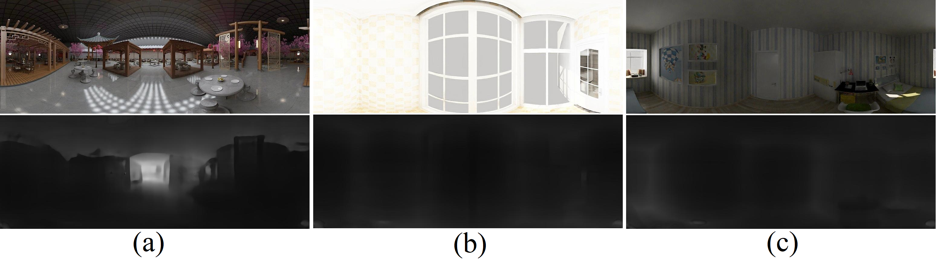
Figure 9: Example of failure cases. HiMODE fails to recover the depth data for complex scenes with (a) many tiny objects, (b) overexposed illumination, and (c) underexposed illumination.

4.6 Limitations

Despite the competitive performance of the proposed HiMODE, it produces some unsatisfactory results in challenging situations. Figure 9 demonstrates some examples where HiMODE fails to generate an accurate depth map. As there are too many fine details and small objects in the complex environment of Figure 9(a), it is challenging to produce a depth map with accurate surface details. In Figure 9(b) and 9(c), extreme illumination (very bright or dark) is shown to degrade the performance of HiMODE.

5 Conclusion

In this paper, we proposed a monocular omnidirectional depth estimator, namely HiMODE. It was designed based on a hybrid architecture of CNN+Transformer to effectively reduce the distortion and artifacts, and recover the surface depth data. The high-level features near the edges were extracted by using a pyramid-based CNN as the backbone, with the HNet block inside. Further performance improvement was achieved by designing SCA block in the Transformer encoder, and STP in the decoder. The sequence length of patch embeddings was reduced when the dimension increased, due to applying the novel structure of SRB after each encoder and decoder. Interestingly, by combining the multi-level deep features extracted from the input images with the depth maps generated by Transformers via the context adjustment layer, HiMODE demonstrated the capability to even recover the lost data in the ground-truth depth maps. Extensive experiments conducted on three benchmark datasets; Stanford3D, Matterport3D, and PanoSunCG, demonstrate that HiMODE can achieve state-of-the-art performance. For future work, we plan to extend HiMODE for real-time monocular $360^{\circ}$ depth estimation, making it robust to illumination changes and efficiently applicable for complex environments. In addition to improving the 3D structure for indoor settings, we would also extend HiMODE for depth estimation and 3D reconstruction for outdoor settings.

Acknowledgements. This work is supported by the Scientific and Technological Research Council of Turkey (TUBITAK) 2232 Leading Researchers Program, Project No. 118C301.

HiMODE: A Hybrid Monocular Omnidirectional Depth Estimation Model
(Supplementary Materials)

In this supplementary material, we provide more ablation studies and results of the proposed HiMODE.

Appendix A Ablation Studies on Backbone

As introduced in the main paper, backbone module is an important part of our system. This section provides more ablation studies on the backbone module to demonstrate its superiority, quantitatively and qualitatively, to the other pre-trained backbones.

A.1 Detailed Architecture of the Backbone.

Our CNN-based backbone is referred to as depth-wise due to using depth-wise Conv layers in HNet blocks which are concatenated with the Conv layers. Depth-wise separable CNNs have less parameters and possibility for overfitting, such as MobileNet. HNet (as shown in Figure 10) is extracted from HardNet [6]. Comparing the number of layers, our backbone has only 40 layers (i.e. HNet=$4\times 8$, Conv=4, Concat=4 layers) which is significantly less than that of HardNet (i.e. 68 layers).

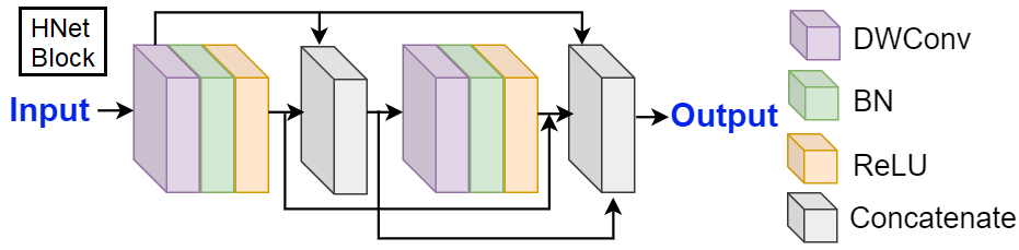
Figure 10: The overall architecture of the proposed HNet block extracted from the HardNet [6] structure.

A.2 The Effects of Input Resolution

The visual information is affected by the image resolution. High image resolution results in higher visual information and so better image quality. Generally, when the image resolution is reduced, the performance of the CNN-based networks degrades significantly [16]. On the other hand, lower input image resolution is desirable as it leads to a reduced number of features and the optimized number of parameters. Consequently, the risk of model overfitting is minimized [4]. Nevertheless, extensive lowering of the image resolution eliminates the information that is useful for classification. The effects of the input image resolution on the overall performance of the proposed system based on our novel CNN-based backbone is investigated and compared with four pre-trained models of ResNet34 [13], ResNet50 [13], DenseNet [15], and HardNet [6]. The evaluation results are presented in Table 6 in terms of four error-based evaluation metrics and three accuracy-based evaluation metrics. The terms ”low” and ”high” for image resolution refer to the image size of $256\times 512$ and $512\times 1024$, respectively. Comparing the results, our proposed backbone ranks first in all evaluation metrics on all three datasets, except for Abs-Rel and $\delta$ on Stanford3D, RMSElog on Matterport3D, and RMSE on PanoSunCG, at which our proposed backbone ranks second with a slight difference. The superiority of our proposed backbone is proven as the other models cannot surpass its performance even with high-resolution inputs. It is worth mentioning that the overall performance of our proposed system maintains almost the same when the resolution of the input images varies, demonstrating its independence and robustness to the input image size. Consequently, our HiMODE system is proposed based on the low-resolution input images so that the number of parameters is reduced without sacrificing the performance accuracy, as opposed to the other state-of-the-art approaches [34, 29] which were mostly based on $512\times 1024$ input images.

A.3 Computation Cost of Different Backbones

In addition to the performance, the superiority of our proposed CNN-based backbone is further investigated by comparing its computation cost with that of four pre-trained models of ResNet34 [13], ResNet50 [13], DenseNet [15], and HardNet [6]. The results in terms of the number of parameters as computation cost with three accuracy-based evaluation metrics on Stanford3D [3] dataset are presented in Table 7 (for both low and high resolution). We can observe that the proposed HiMODE based on our novel CNN-based backbone has the least number of parameters for low resolution input images with the values of 79.67M as well as the best performance accuracy of 0.9711 and 0.9965 in terms of $\delta$, $\delta^{2}$, respectively. Its performance in terms of $\delta^{3}$ is almost the same as that of HardNet. Replacing the other pre-trained models of ResNet34, ResNet50, DenseNet, and HardNet with our proposed backbone brings additional computation burden (i.e. parameters) of 7.29M, 10M, 6.48M, and 2.57M, respectively. Besides, accuracy also significantly decreases. The highest degradation in $\delta$, and $\delta^{2}$ occurs in DenseNet with the values of 0.9076 and 0.9839, respectively, while the poorest performance of 0.9880 in terms of $\delta^{3}$ belongs to ResNet34. For high resolution input images, HiMODE based on our proposed CNN-based backbone still has the least number of parameters (98.89M) comparing with the others. Achieving the least computation cost with the highest performance accuracy proves the capabilities of our proposed backbone over the other pre-trained feature extractors.

Table 6: A quantitative comparison between the proposed CNN-based backbone with four pre-trained models on three datasets based on two input image resolutions of $256\times 512$ (low) and $512\times 1024$ (high).

Datasets	Backbones	Resolution	Errors				Accuracy
			Abs-Rel	Sq-Rel	RMSE	RMSElog	$\delta$	$\delta^{2}$	$\delta^{3}$
Stanford3D	ResNet34 [13]	High	0.0956	0.0824	0.3875	0.1577	0.9398	0.9817	0.9906
		Low	0.1128	0.0635	0.3665	0.1873	0.9149	0.9884	0.9880
	ResNet50 [13]	High	0.0666	0.0489	0.2897	0.1217	0.9512	0.9940	0.9968
		Low	0.0509	0.0682	0.3177	0.1185	0.9349	0.9906	0.9923
	DenseNet [15]	High	0.0823	0.0702	0.3346	0.1246	0.9451	0.9901	0.9944
		Low	0.1045	0.0624	0.3358	0.1621	0.9076	0.9839	0.9889
	HardNet [6]	High	0.0755	0.0461	0.2984	0.1038	0.9578	0.9947	0.9972
		Low	0.0789	0.0352	0.3041	0.1215	0.9234	0.9947	0.9992
	Proposed	High	0.0679	0.0223	0.2711	0.0963	0.9693	0.9959	0.9987
		Low	0.0532	0.0207	0.2619	0.0821	0.9711	0.9965	0.9989
Matterport3D	ResNet34 [13]	High	0.1026	0.0861	0.3956	0.1434	0.9487	0.9820	0.9777
		Low	0.1078	0.1139	0.4587	0.1786	0.8976	0.9792	0.9800
	ResNet50 [13]	High	0.0699	0.0586	0.3610	0.1003	0.9523	0.9928	0.9859
		Low	0.1014	0.0856	0.4189	0.1251	0.9257	0.9755	0.9945
	DenseNet [15]	High	0.0782	0.0545	0.3678	0.1165	0.9501	0.9893	0.9908
		Low	0.0935	0.0472	0.3548	0.1547	0.9138	0.9668	0.9829
	HardNet [6]	High	0.0630	0.0471	0.3355	0.0873	0.9562	0.9918	0.9938
		Low	0.0769	0.0244	0.3648	0.1174	0.9415	0.9831	0.9902
	Proposed	High	0.0597	0.0213	0.3146	0.0894	0.9601	0.9921	0.9981
		Low	0.0658	0.0245	0.3067	0.0959	0.9608	0.9940	0.9985
PanoSunCG	ResNet34 [13]	High	0.1006	0.0653	0.3989	0.1595	0.9466	0.9783	0.9849
		Low	0.1353	0.1471	0.4823	0.2379	0.9183	0.9947	0.9926
	ResNet50 [13]	High	0.0832	0.0474	0.3259	0.1339	0.9524	0.9864	0.9936
		Low	0.1094	0.1043	0.3847	0.2149	0.9524	0.9918	0.9989
	DenseNet [15]	High	0.0852	0.0427	0.3561	0.1226	0.9538	0.9889	0.9951
		Low	0.0949	0.0987	0.4283	0.1958	0.9245	0.9909	0.9895
	HardNet [6]	High	0.0715	0.0398	0.3303	0.1178	0.9615	0.9910	0.9978
		Low	0.0726	0.0557	0.3985	0.1305	0.9693	0.9897	0.9877
	Proposed	High	0.0667	0.0347	0.3265	0.1013	0.9691	0.9945	0.9990
		Low	0.0682	0.0356	0.3378	0.1048	0.9688	0.9951	0.9992

Table 7: Comparison between the proposed CNN-based backbone with four pre-trained models as backbone in terms of computation cost and accuracy (on Stanford3D dataset). The bold and underlined numbers indicate the best results for low and high resolution input images, respectively.

Backbones	Input	Computation Cost	Accuracy
		Parameters	$\delta$	$\delta^{2}$	$\delta^{3}$
ResNet34 [13]	High	103.55M	0.9398	0.9817	0.9906
	Low	86.96M	0.9149	0.9884	0.9880
ResNet50 [13]	High	107.28M	0.9512	0.9940	0.9968
	Low	89.67M	0.9349	0.9906	0.9923
DenseNet [15]	High	104.81M	0.9451	0.9901	0.9944
	Low	86.15M	0.9076	0.9839	0.9889
HardNet [6]	High	100.37M	0.9578	0.9947	0.9972
	Low	82.24M	0.9234	0.9947	0.9992
Proposed	High	98.89M	0.9693	0.9959	0.9987
	Low	79.67M	0.9711	0.9965	0.9989

Table 8: Quantitative comparison between our HiMODE and five state-of-the-art methods for 3D structure estimation on Stanford3D dataset in terms of 2D and 3D IOU. The best results are indicated with bold numbers.

IOU (%)	Approaches	# Corners
		All	4	6	8	$10+$
2D	LayoutNet v2 [45]	$75.82$	$81.35$	$72.33$	$67.45$	$63.00$
	DuLa-Net v2 [38]	$75.07$	$77.02$	$78.79$	$71.03$	$63.27$
	HorizonNet [28]	$79.11$	$81.88$	82.26	$71.78$	$68.32$
	AtlantaNet [24]	80.02	$82.09$	$82.08$	75.19	71.61
	HoHoNet [29]	$79.88$	82.64	$82.16$	$73.65$	$69.26$
	HiMODE	$79.74$	$82.40$	82.23	$72.87$	$69.03$
3D	LayoutNet v2 [45]	$78.73$	$84.61$	$75.02$	$69.79$	$65.14$
	DuLa-Net v2 [38]	$78.82$	$81.12$	$82.69$	$74.00$	$66.12$
	HorizonNet [28]	$81.71$	$84.67$	84.82	$73.91$	$70.58$
	AtlantaNet [24]	$82.09$	$84.42$	$83.85$	76.97	73.18
	HoHoNet [29]	82.32	$85.26$	$84.81$	$75.59$	$70.98$
	HiMODE	$81.41$	85.48	85.05	$74.38$	$70.10$

A.4 Qualitative Results for Different Backbones

The performance of HiMODE based on our proposed CNN-based backbone is compared with the other pre-trained models qualitatively in Figures 11-13. As it is mentioned in the main paper, our depth-wise proposed backbone can extract high-resolution features near the edges to overcome distortion and artifact issues. On the depth maps estimated based on our proposed backbone, sharper edges and more details are recovered.

Appendix B More Results on 3D Structure

B.1 Quantitative Results

The detailed quantitative results for 3D structure estimation under different number of ground-truth corners are presented in Table 8 as a supplement to the main paper to extend the quantitative studies. In comparison with the recent state-of-the-art approaches, our proposed HiMODE achieves the best results for 6 corners (82.23%) on the 2D IOU (intersection over union) metric, and both 4 (85.48%) and 6 (85.05%) corners in terms of 3D IOU. Overall, our proposed method can achieve state-of-the-art performance in 3D structure estimation with fewer corners. For higher number of corners, our method obtained comparable results although AtlantaNet [24] is the best performer.

Input Image              ResNet34              ResNet50              DenseNet                  HardNet                 Proposed

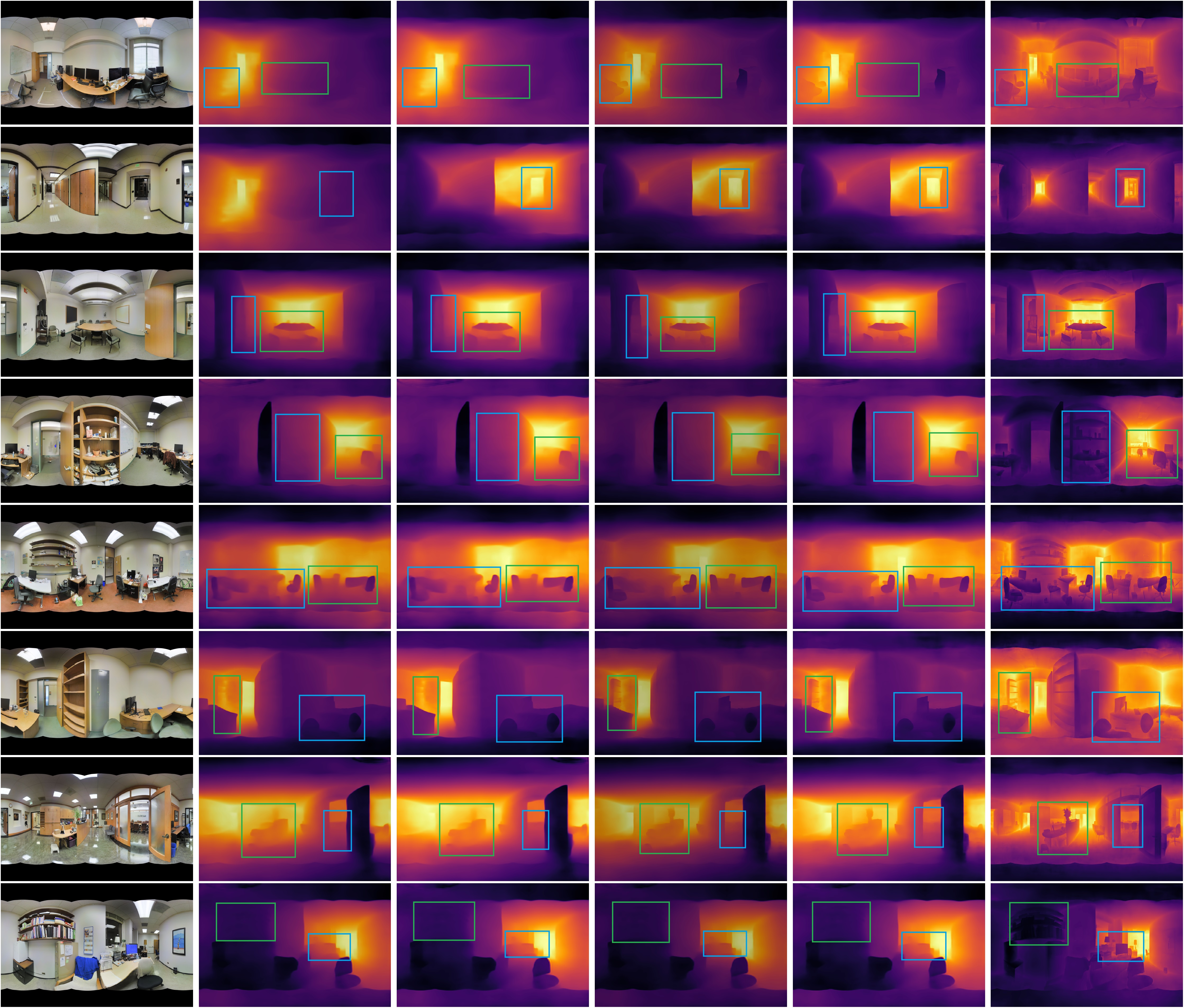
Figure 11: Qualitative comparisons for our HiMODE based on our proposed CNN-based backbone and four pre-trained models of ResNet34 [13], ResNet50 [13], DenseNet [15], and HardNet [6] on Stanford3D dataset. As demonstrated by rectangles, our HiMODE can accurately recover the details of the surface especially sharp edges even for the deep regions and small objects.

Input Image              ResNet34              ResNet50              DenseNet                  HardNet                 Proposed

Figure 12: Qualitative comparisons for our HiMODE based on our proposed CNN-based backbone and four pre-trained models of ResNet34 [13], ResNet50 [13], DenseNet [15], and HardNet [6] on Matterport3D dataset. As demonstrated by rectangles, our HiMODE can accurately recover the details of the surface especially sharp edges even for the deep regions and small objects.

Input Image              ResNet34              ResNet50              DenseNet                  HardNet                 Proposed

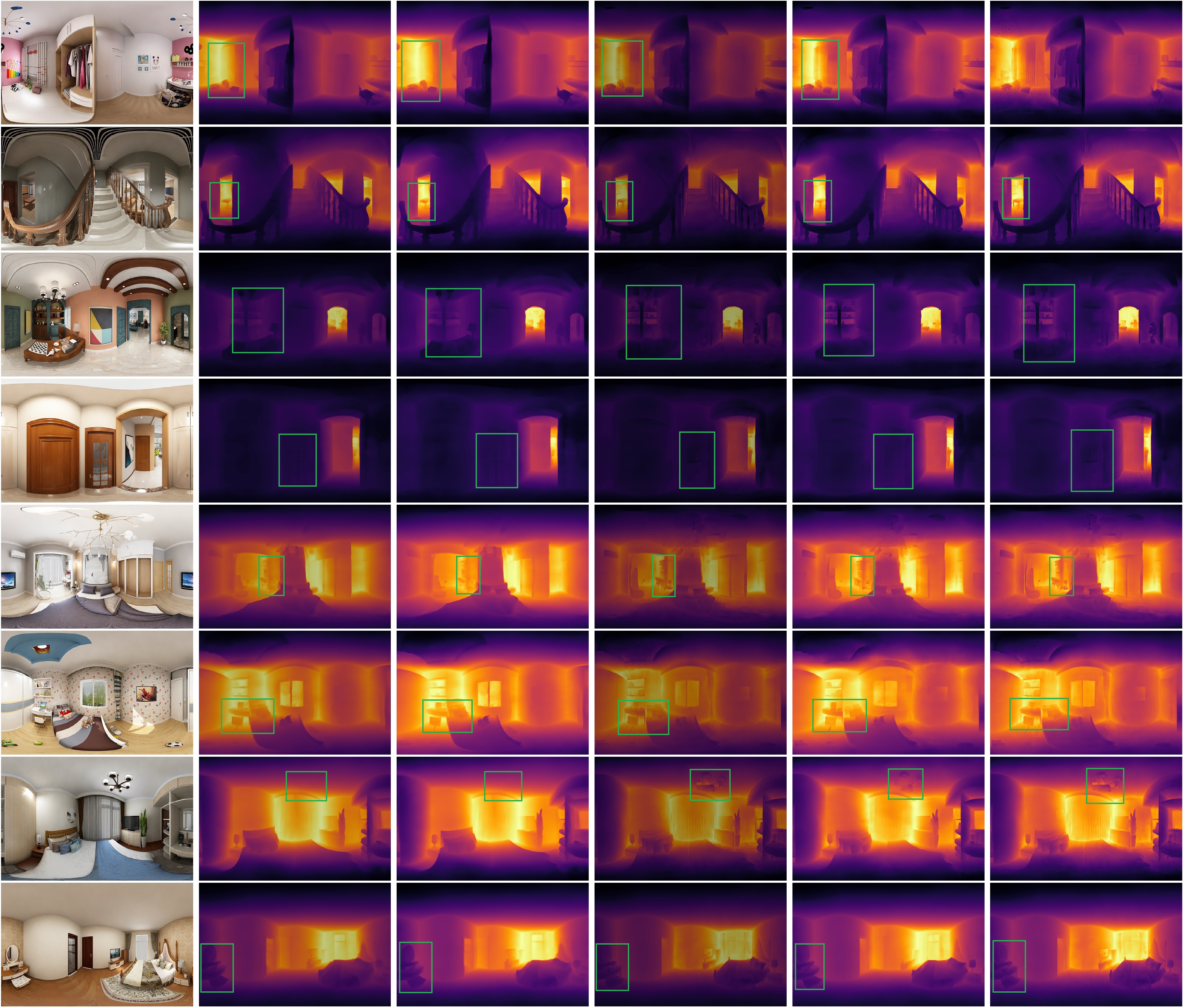
Figure 13: Qualitative comparisons for our HiMODE based on our proposed CNN-based backbone and four pre-trained models of ResNet34 [13], ResNet50 [13], DenseNet [15], and HardNet [6] on PanoSunCG dataset. As demonstrated by rectangles, our HiMODE can accurately recover the details of the surface especially sharp edges even for the deep regions and small objects.

B.2 Qualitative Results

Additional qualitative results for estimating 3D structures from monocular omnidirectional images on three datsets of Stanford3D [3], Matterport3D [5], and PanoSunCG [33] are demonstrated in Figures 14-16, respectively. Our method was evaluated on different input images with various numbers of corners. Qualitatively, our HiMODE can successfully reconstruct the 3D structure by finding the corners and boundary between walls, floor, and ceiling, which is a vital task in VR/AR and robotics applications. The proposed HiMODE successfully reconstructs the 3D structure with different numbers of corners by finding the corners and boundary between walls, floor, and ceiling.

Input Image                   3D View: Angle 1                 3D View: Angle 2                 3D View: Angle 3

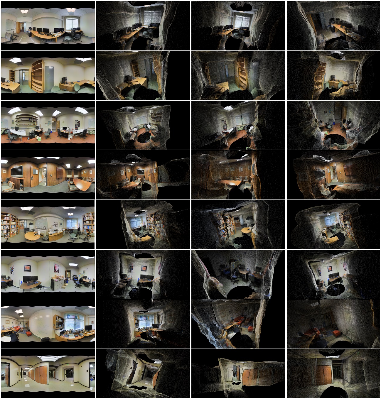
Figure 14: 3D structures estimation on Stanford3D dataset using our HiMODE.

Input Image                   3D View: Angle 1                 3D View: Angle 2                 3D View: Angle 3

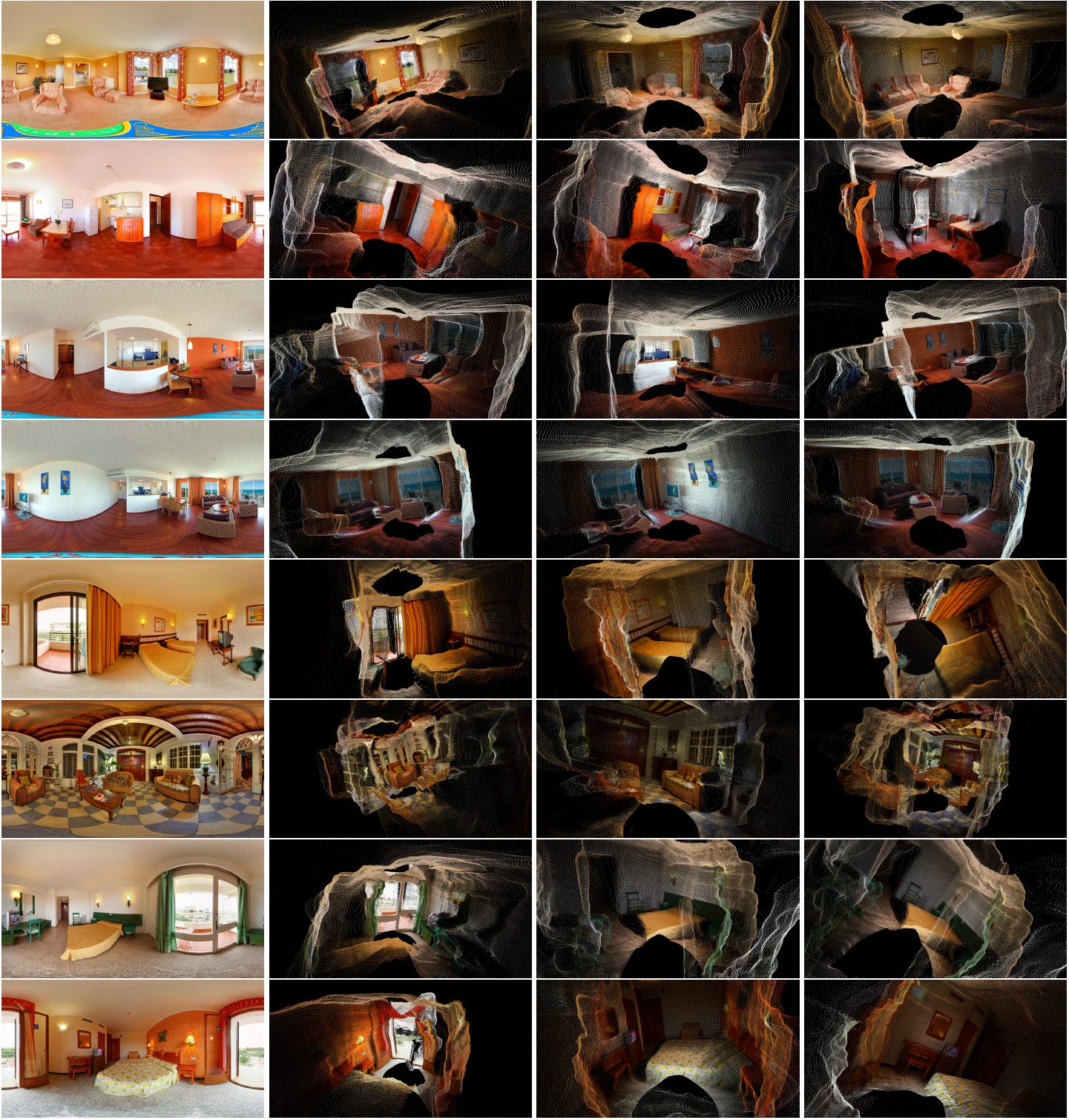
Figure 15: 3D structures estimation on Matterport3D dataset using our HiMODE.

Input Image                   3D View: Angle 1                 3D View: Angle 2                 3D View: Angle 3

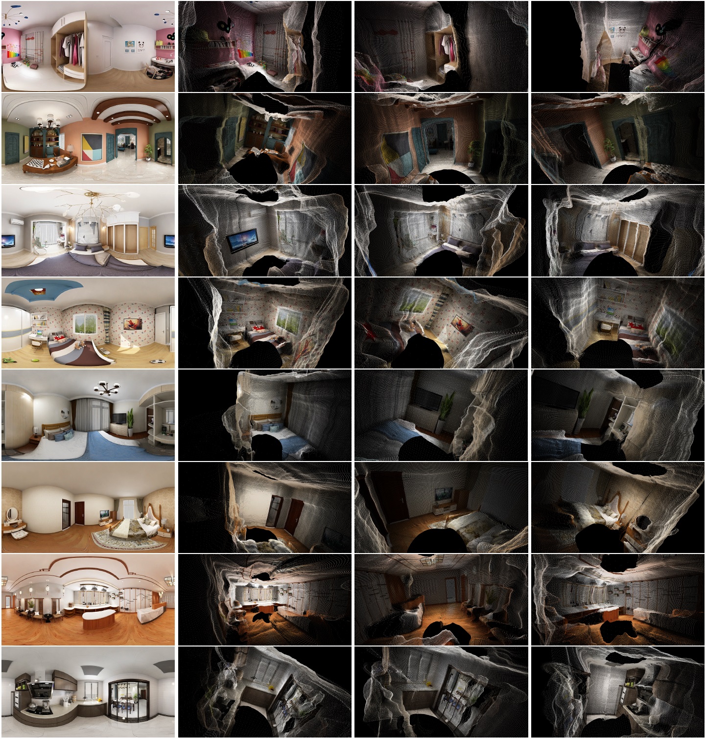
Figure 16: 3D structures estimation on PanoSunCG dataset using our HiMODE.

Appendix C More Omnidirectional Depth Results

We show more qualitative results for depth map estimation by our HiMODE in Figures 17-19 on three datasets; Stanford3D, Matterport3D, and PanoSunCG. The results of our proposed HiMODE are compared with two other recent state-of-the-art approaches of Bifuse [34] and HoHoNet [29] on three datasets in Figures 20-22. These visual results further demonstrate the superior performance of the proposed HiMODE over the other two methods in recovering the details of the surfaces, even for the deep regions and small objects.

In addition, the effectiveness of combining the HiMODE output with the output of two recent state-of-the-art approaches; Bifuse [34] and HoHoNet [29], on three datasets is investigated. The qualitative results are illustrated in Figures 23-25. Very interestingly, we observe significant improvement in the depth map estimation when HiMODE is combined with Bifuse, HohoNet, or both methods via a simple concatenation of the respective outputs. The best qualitative results are achieved with the combination of three methods, whereby the resulting depth map mimics the groundtruth depth map very closely (the last columns of Figures 23-25).

Input Image                             G.T                      HiMODE (gray-scale)               HiMODE (color)

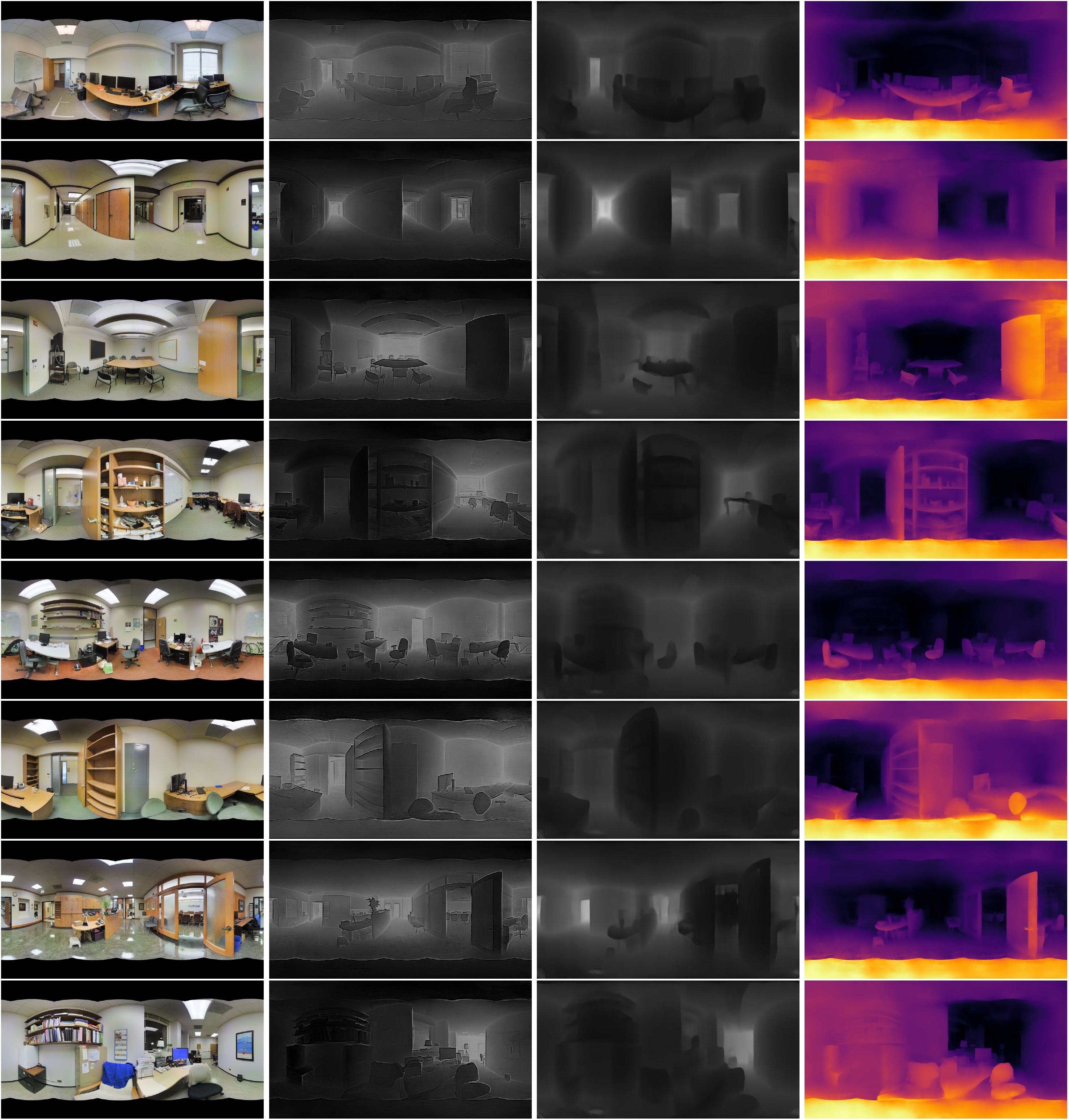
Figure 17: More qualitative results for omnidirectional depth map estimation based on our HiMODE on Stanford3D dataset.

Input Image                             G.T                      HiMODE (gray-scale)               HiMODE (color)

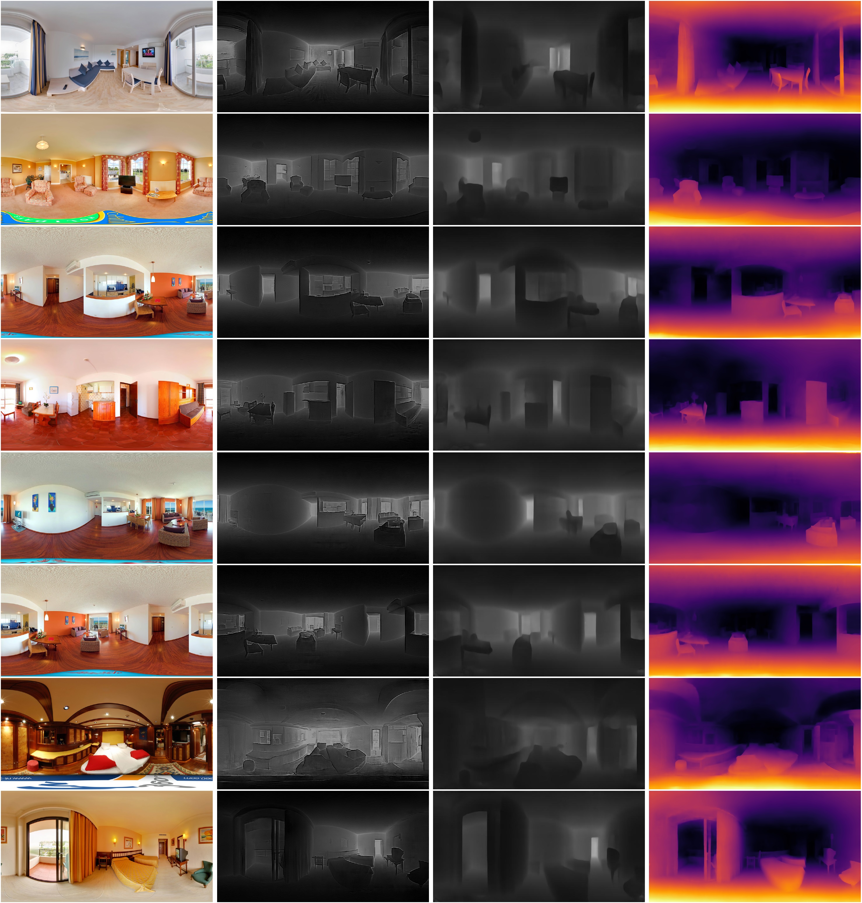
Figure 18: More qualitative results for omnidirectional depth map estimation based on our HiMODE on Matterport3D dataset.

Input Image                             G.T                      HiMODE (gray-scale)               HiMODE (color)

Figure 19: More qualitative results for omnidirectional depth map estimation based on our HiMODE on PanoSunCG dataset.

Input Image                           Bifuse                             HoHoNet                          HiMODE

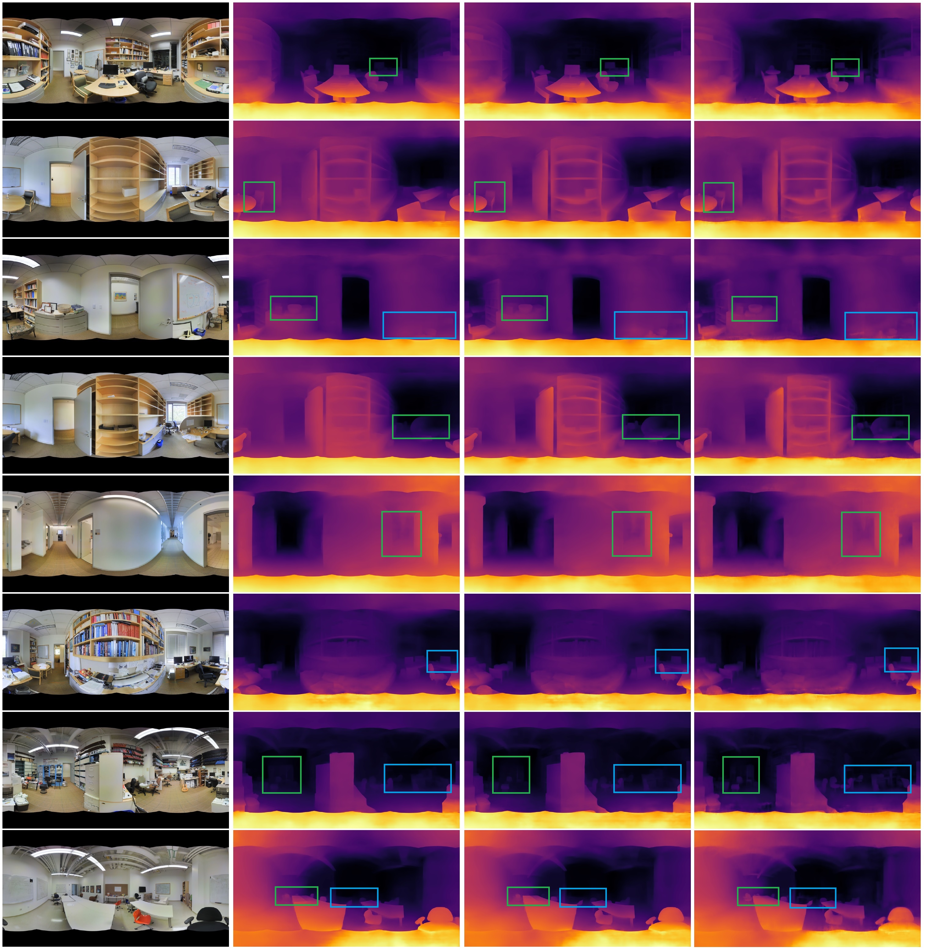
Figure 20: More qualitative comparisons between our HiMODE and two recent state-of-the-art approaches, Bifuse [34] and HoHoNet [29] on Stanford3D dataset. As demonstrated by rectangles, our HiMODE can accurately recover the details of the surface even for the deep regions with small objects.

Input Image                           Bifuse                             HoHoNet                          HiMODE

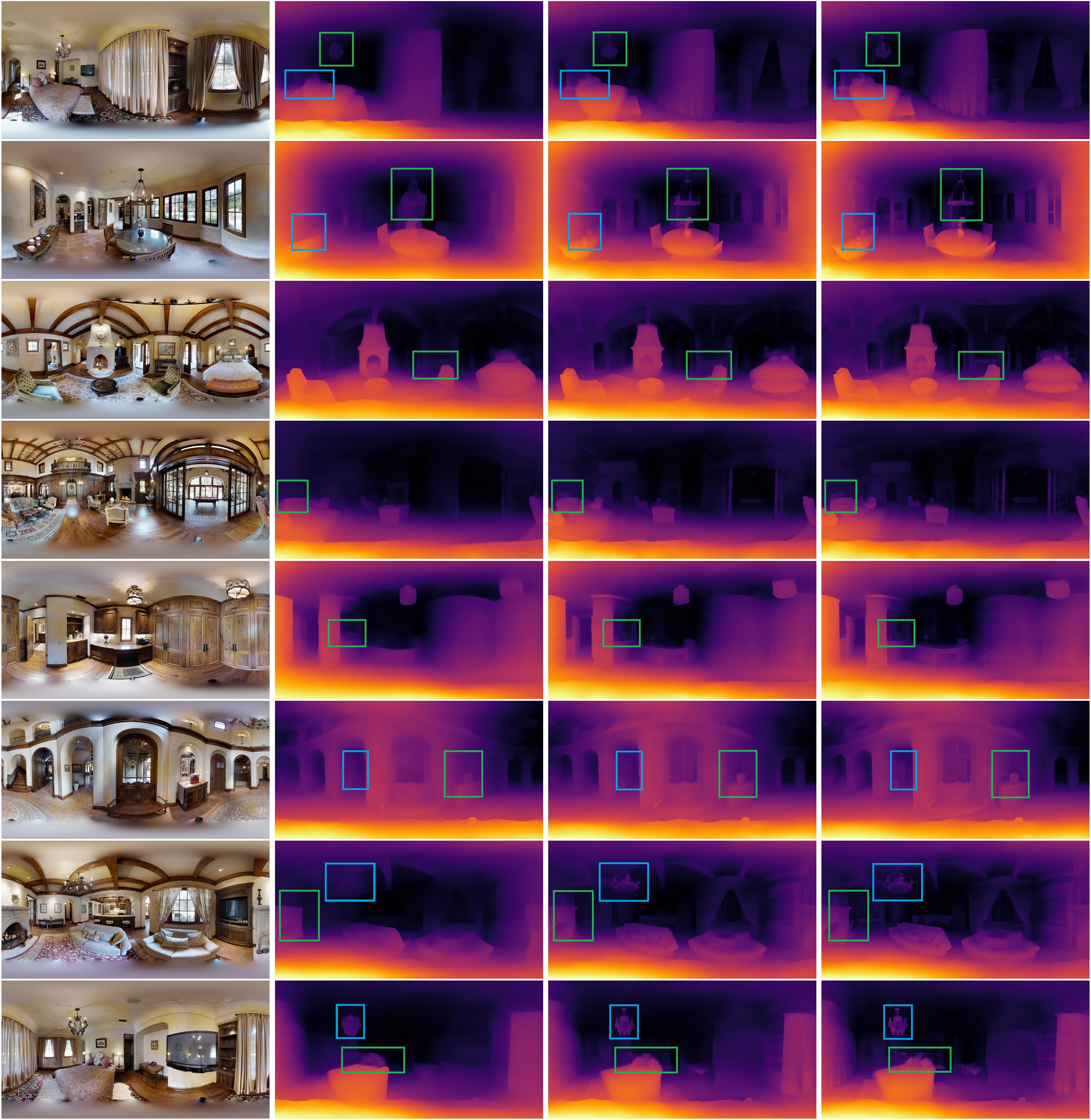
Figure 21: More qualitative comparisons between our HiMODE and two recent state-of-the-art approaches, Bifuse [34] and HoHoNet [29] on Matterport3D dataset. As demonstrated by rectangles, our HiMODE can accurately recover the details of the surface with sharp edges even for the deep regions and for small objects.

Input Image                           Bifuse                             HoHoNet                          HiMODE

Figure 22: More qualitative comparisons between our HiMODE and two recent state-of-the-art approaches, Bifuse [34] and HoHoNet [29] on PanoSunCG dataset. As demonstrated by rectangles, our HiMODE can accurately recover the details of the surface with sharp edges even for the deep regions and for small objects.

Input Image               G.T                  HiMODE          Bifuse + HiMODE    HoHoNet + HiMODE            All

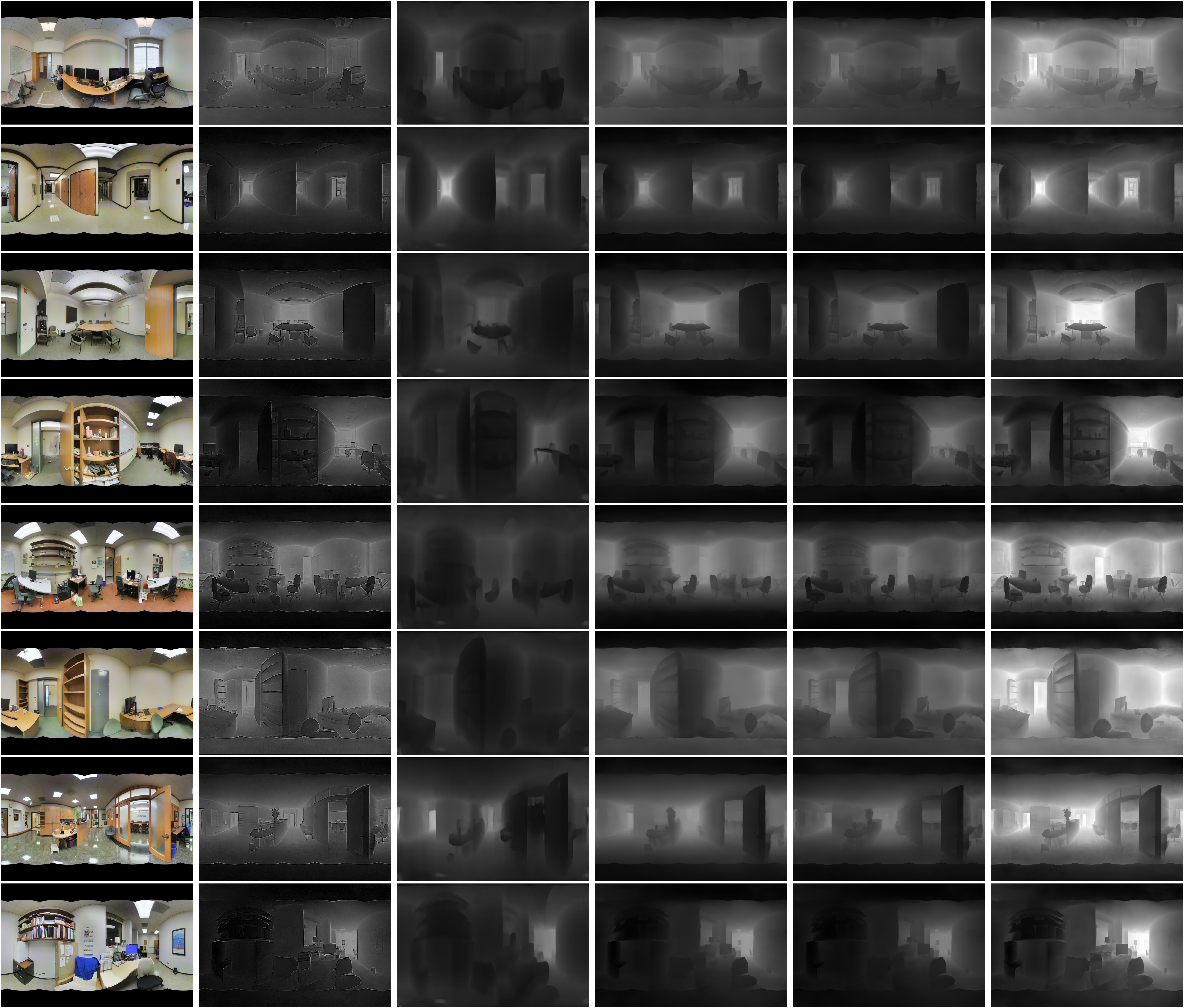
Figure 23: More qualitative results for omnidirectional depth map estimation based on our HiMODE along with its combination with two recent state-of-the-art approaches, Bifuse [34] and HoHoNet [29] on Stanford3D dataset.

Input Image               G.T                  HiMODE          Bifuse + HiMODE    HoHoNet + HiMODE            All

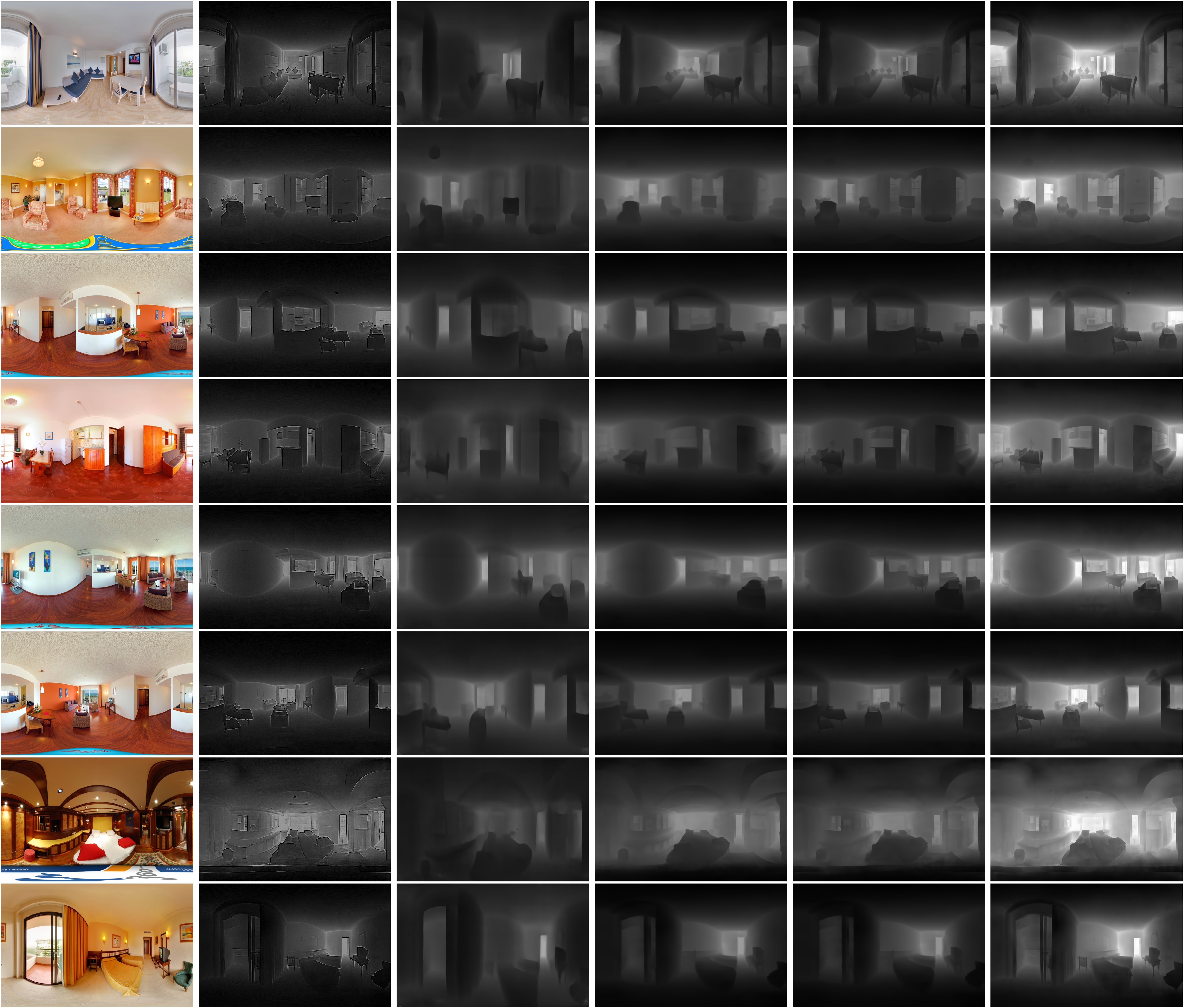
Figure 24: More qualitative results for omnidirectional depth map estimation based on our HiMODE along with its combination with two recent state-of-the-art approaches, Bifuse [34] and HoHoNet [29] on Matterport3D dataset.

Input Image               G.T                  HiMODE          Bifuse + HiMODE    HoHoNet + HiMODE            All

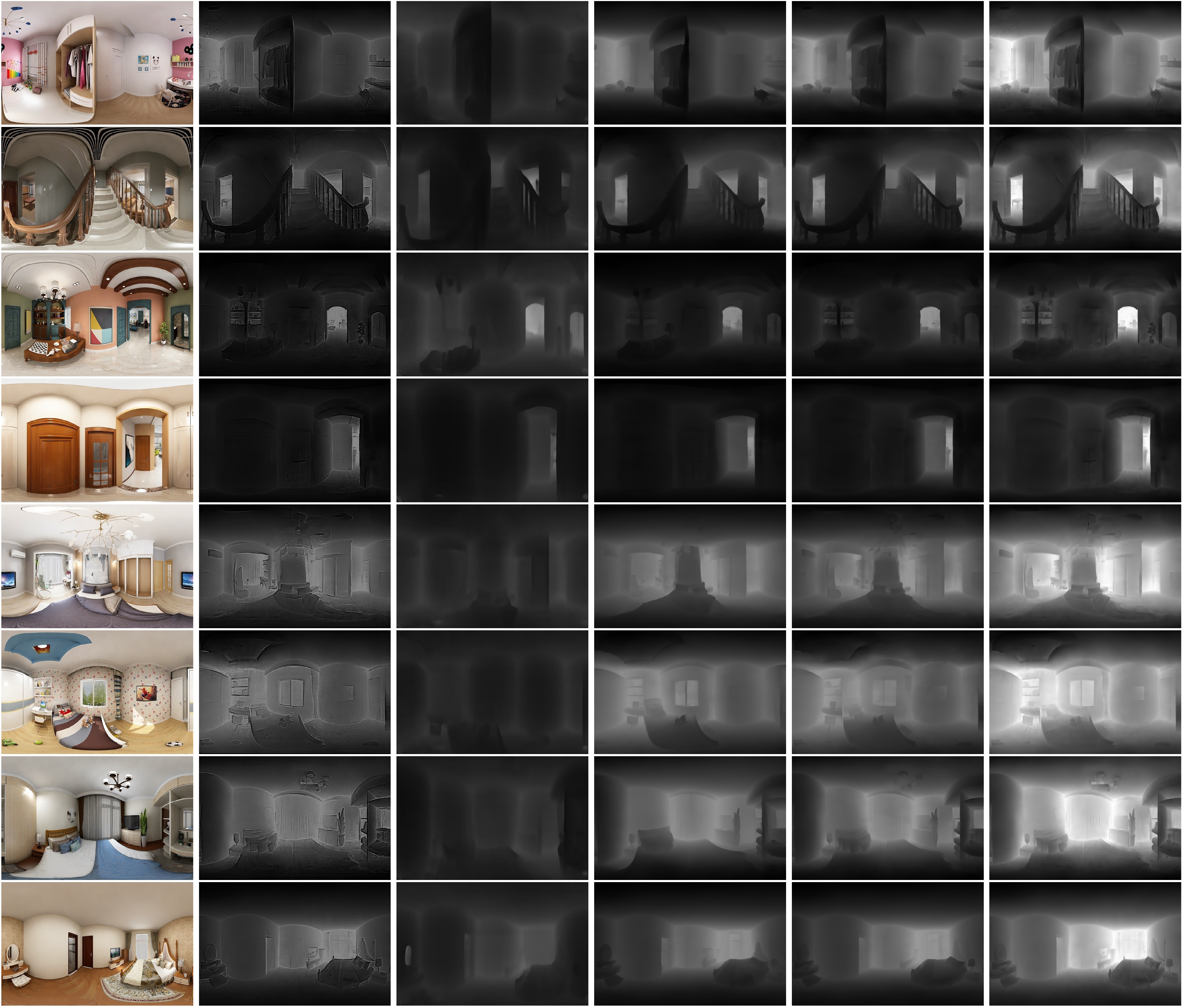
Figure 25: More qualitative results for omnidirectional depth map estimation based on our HiMODE along with its combination with two recent state-of-the-art approaches, Bifuse [34] and HoHoNet [29] on PanoSunCG dataset.

References

- [1] Georgios Albanis, Nikolaos Zioulis, Petros Drakoulis, Vasileios Gkitsas, Vladimiros Sterzentsenko, Federico Alvarez, Dimitrios Zarpalas, and Petros Daras. Pano3d: A holistic benchmark and a solid baseline for 360° depth estimation. In 2021 IEEE/CVF Conference on Computer Vision and Pattern Recognition Workshops (CVPRW), pages 3722–3732. IEEE, 2021.
- [2] Lemonia Argyriou, Daphne Economou, and Vassiliki Bouki. Design methodology for 360 immersive video applications: the case study of a cultural heritage virtual tour. Personal and Ubiquitous Computing, 24(6):843–859, 2020.
- [3] Iro Armeni, Sasha Sax, Amir R Zamir, and Silvio Savarese. Joint 2d-3d-semantic data for indoor scene understanding. arXiv preprint arXiv:1702.01105, 2017.
- [4] Roberto Battiti. Using mutual information for selecting features in supervised neural net learning. IEEE Transactions on neural networks, 5(4):537–550, 1994.
- [5] Angel Chang, Angela Dai, Thomas Funkhouser, Maciej Halber, Matthias Niessner, Manolis Savva, Shuran Song, Andy Zeng, and Yinda Zhang. Matterport3d: Learning from rgb-d data in indoor environments. arXiv preprint arXiv:1709.06158, 2017.
- [6] Ping Chao, Chao-Yang Kao, Yu-Shan Ruan, Chien-Hsiang Huang, and Youn-Long Lin. Hardnet: A low memory traffic network. In Proceedings of the IEEE/CVF International Conference on Computer Vision, pages 3552–3561, 2019.
- [7] Xinjing Cheng, Peng Wang, Yanqi Zhou, Chenye Guan, and Ruigang Yang. Omnidirectional depth extension networks. In 2020 IEEE International Conference on Robotics and Automation (ICRA), pages 589–595. IEEE, 2020.
- [8] Alexey Dosovitskiy, Lucas Beyer, Alexander Kolesnikov, Dirk Weissenborn, Xiaohua Zhai, Thomas Unterthiner, Mostafa Dehghani, Matthias Minderer, Georg Heigold, Sylvain Gelly, et al. An image is worth 16x16 words: Transformers for image recognition at scale. arXiv preprint arXiv:2010.11929, 2020.
- [9] Marc Eder, Pierre Moulon, and Li Guan. Pano popups: Indoor 3d reconstruction with a plane-aware network. In 2019 International Conference on 3D Vision (3DV), pages 76–84. IEEE, 2019.
- [10] David Eigen, Christian Puhrsch, and Rob Fergus. Depth map prediction from a single image using a multi-scale deep network. arXiv preprint arXiv:1406.2283, 2014.
- [11] Huan Fu, Mingming Gong, Chaohui Wang, Kayhan Batmanghelich, and Dacheng Tao. Deep ordinal regression network for monocular depth estimation. In Proceedings of the IEEE conference on computer vision and pattern recognition, pages 2002–2011, 2018.
- [12] Mozhdeh Gheini, Xiang Ren, and Jonathan May. Cross-attention is all you need: Adapting pretrained transformers for machine translation. arXiv preprint arXiv:2104.08771, 2021.
- [13] Kaiming He, Xiangyu Zhang, Shaoqing Ren, and Jian Sun. Deep residual learning for image recognition. In Proceedings of the IEEE conference on computer vision and pattern recognition, pages 770–778, 2016.
- [14] Junjie Hu, Mete Ozay, Yan Zhang, and Takayuki Okatani. Revisiting single image depth estimation: Toward higher resolution maps with accurate object boundaries. In 2019 IEEE Winter Conference on Applications of Computer Vision (WACV), pages 1043–1051. IEEE, 2019.
- [15] Gao Huang, Zhuang Liu, Laurens Van Der Maaten, and Kilian Q Weinberger. Densely connected convolutional networks. In Proceedings of the IEEE conference on computer vision and pattern recognition, pages 4700–4708, 2017.
- [16] Suresh Prasad Kannojia and Gaurav Jaiswal. Effects of varying resolution on performance of cnn based image classification: An experimental study. Int. J. Comput. Sci. Eng, 6(9):451–456, 2018.
- [17] Po Kong Lai, Shuang Xie, Jochen Lang, and Robert Laganière. Real-time panoramic depth maps from omni-directional stereo images for 6 dof videos in virtual reality. In 2019 IEEE Conference on Virtual Reality and 3D User Interfaces (VR), pages 405–412. IEEE, 2019.
- [18] Iro Laina, Christian Rupprecht, Vasileios Belagiannis, Federico Tombari, and Nassir Navab. Deeper depth prediction with fully convolutional residual networks. In 2016 Fourth international conference on 3D vision (3DV), pages 239–248. IEEE, 2016.
- [19] Jae-Han Lee and Chang-Su Kim. Multi-loss rebalancing algorithm for monocular depth estimation. In Computer Vision–ECCV 2020: 16th European Conference, Glasgow, UK, August 23–28, 2020, Proceedings, Part XVII 16, pages 785–801. Springer, 2020.
- [20] Yuyan Li, Zhixin Yan, Ye Duan, and Liu Ren. Panodepth: A two-stage approach for monocular omnidirectional depth estimation.
- [21] Chen Liu, Jimei Yang, Duygu Ceylan, Ersin Yumer, and Yasutaka Furukawa. Planenet: Piece-wise planar reconstruction from a single rgb image. In Proceedings of the IEEE Conference on Computer Vision and Pattern Recognition, pages 2579–2588, 2018.
- [22] Michele Mancini, Gabriele Costante, Paolo Valigi, and Thomas A Ciarfuglia. J-mod 2: Joint monocular obstacle detection and depth estimation. IEEE Robotics and Automation Letters, 3(3):1490–1497, 2018.
- [23] Anwesan Pal, Sayan Mondal, and Henrik I Christensen. ” looking at the right stuff”-guided semantic-gaze for autonomous driving. In Proceedings of the IEEE/CVF Conference on Computer Vision and Pattern Recognition, pages 11883–11892, 2020.
- [24] Giovanni Pintore, Marco Agus, and Enrico Gobbetti. Atlantanet: Inferring the 3d indoor layout from a single image beyond the manhattan world assumption. In European Conference on Computer Vision, pages 432–448. Springer, 2020.
- [25] Giovanni Pintore, Claudio Mura, Fabio Ganovelli, Lizeth Fuentes-Perez, Renato Pajarola, and Enrico Gobbetti. State-of-the-art in automatic 3d reconstruction of structured indoor environments. In Computer Graphics Forum, volume 39, pages 667–699. Wiley Online Library, 2020.
- [26] Weijing Shi and Raj Rajkumar. Point-gnn: Graph neural network for 3d object detection in a point cloud. In Proceedings of the IEEE/CVF conference on computer vision and pattern recognition, pages 1711–1719, 2020.
- [27] Nathan Silberman, Derek Hoiem, Pushmeet Kohli, and Rob Fergus. Indoor segmentation and support inference from rgbd images. In European conference on computer vision, pages 746–760. Springer, 2012.
- [28] Cheng Sun, Chi-Wei Hsiao, Min Sun, and Hwann-Tzong Chen. Horizonnet: Learning room layout with 1d representation and pano stretch data augmentation. In Proceedings of the IEEE/CVF Conference on Computer Vision and Pattern Recognition, pages 1047–1056, 2019.
- [29] Cheng Sun, Min Sun, and Hwann-Tzong Chen. Hohonet: 360 indoor holistic understanding with latent horizontal features. In Proceedings of the IEEE/CVF Conference on Computer Vision and Pattern Recognition, pages 2573–2582, 2021.
- [30] Keisuke Tateno, Nassir Navab, and Federico Tombari. Distortion-aware convolutional filters for dense prediction in panoramic images. In Proceedings of the European Conference on Computer Vision (ECCV), pages 707–722, 2018.
- [31] Hugo Touvron, Matthieu Cord, Matthijs Douze, Francisco Massa, Alexandre Sablayrolles, and Hervé Jégou. Training data-efficient image transformers & distillation through attention. In International Conference on Machine Learning, pages 10347–10357. PMLR, 2021.
- [32] Ashish Vaswani, Noam Shazeer, Niki Parmar, Jakob Uszkoreit, Llion Jones, Aidan N Gomez, Łukasz Kaiser, and Illia Polosukhin. Attention is all you need. In Advances in neural information processing systems, pages 5998–6008, 2017.
- [33] Fu-En Wang, Hou-Ning Hu, Hsien-Tzu Cheng, Juan-Ting Lin, Shang-Ta Yang, Meng-Li Shih, Hung-Kuo Chu, and Min Sun. Self-supervised learning of depth and camera motion from videos. In Asian Conference on Computer Vision, pages 53–68. Springer, 2018.
- [34] Fu-En Wang, Yu-Hsuan Yeh, Min Sun, Wei-Chen Chiu, and Yi-Hsuan Tsai. Bifuse: Monocular 360 depth estimation via bi-projection fusion. In Proceedings of the IEEE/CVF Conference on Computer Vision and Pattern Recognition, pages 462–471, 2020.
- [35] Peng Wang, Xiaohui Shen, Zhe Lin, Scott Cohen, Brian Price, and Alan L Yuille. Towards unified depth and semantic prediction from a single image. In Proceedings of the IEEE conference on computer vision and pattern recognition, pages 2800–2809, 2015.
- [36] Di Xu, Xiaojun Liu, and Yanning Zhang. Real-time depth estimation for aerial panoramas in virtual reality. In 2020 IEEE Conference on Virtual Reality and 3D User Interfaces Abstracts and Workshops (VRW), pages 704–705. IEEE, 2020.
- [37] Dan Xu, Wanli Ouyang, Xiaogang Wang, and Nicu Sebe. Pad-net: Multi-tasks guided prediction-and-distillation network for simultaneous depth estimation and scene parsing. In Proceedings of the IEEE Conference on Computer Vision and Pattern Recognition, pages 675–684, 2018.
- [38] Shang-Ta Yang, Fu-En Wang, Chi-Han Peng, Peter Wonka, Min Sun, and Hung-Kuo Chu. Dula-net: A dual-projection network for estimating room layouts from a single rgb panorama. In Proceedings of the IEEE/CVF Conference on Computer Vision and Pattern Recognition, pages 3363–3372, 2019.
- [39] Xin Yang, Qingling Chang, Xinglin Liu, Siyuan He, and Yan Cui. Monocular depth estimation based on multi-scale depth map fusion. IEEE Access, 9:67696–67705, 2021.
- [40] Yang Yang, Shi Jin, Ruiyang Liu, Sing Bing Kang, and Jingyi Yu. Automatic 3d indoor scene modeling from single panorama. In Proceedings of the IEEE Conference on Computer Vision and Pattern Recognition, pages 3926–3934, 2018.
- [41] Ilwi Yun, Hyuk-Jae Lee, and Chae Eun Rhee. Improving 360 monocular depth estimation via non-local dense prediction transformer and joint supervised and self-supervised learning. arXiv preprint arXiv:2109.10563, 2021.
- [42] Yanhong Zeng, Jianlong Fu, and Hongyang Chao. Learning joint spatial-temporal transformations for video inpainting. In European Conference on Computer Vision, pages 528–543. Springer, 2020.
- [43] Nikolaos Zioulis, Antonis Karakottas, Dimitrios Zarpalas, Federico Alvarez, and Petros Daras. Spherical view synthesis for self-supervised 360 depth estimation. In 2019 International Conference on 3D Vision (3DV), pages 690–699. IEEE, 2019.
- [44] Nikolaos Zioulis, Antonis Karakottas, Dimitrios Zarpalas, and Petros Daras. Omnidepth: Dense depth estimation for indoors spherical panoramas. In Proceedings of the European Conference on Computer Vision (ECCV), pages 448–465, 2018.
- [45] Chuhang Zou, Jheng-Wei Su, Chi-Han Peng, Alex Colburn, Qi Shan, Peter Wonka, Hung-Kuo Chu, and Derek Hoiem. 3d manhattan room layout reconstruction from a single 360 image. 2019.