Daily Generation Scheduling :Decomposition Methods to Solve the Hydraulic Problems

Abstract

Short-term hydro-generation management poses a non-convex or even non-continuous optimization problem. For this reason, the problem of systematically obtaining feasible and economically satisfying solutions has not yet been completely solved.

Two decomposition methods, which, as far as we know, have not been applied in this field, are here proposed :

• the first is based on a decomposition by prediction method and the coordination is a primal-dual relaxation algorithm,

• handling the dynamic constraints by duality, the second achieves a price decomposition by an Augmented Lagrangian technique.

Numerical tests show the efficiency of these algorithms. They will enable the process in use at Electricité de France to be improved.

Keywords

Hydro-thermal scheduling, Decomposition methods.

1 Introduction

The optimization of a hydro-valley’s daily generation schedules poses a problem of an appreciable size. For instance, a problem related to a valley of five or six reserves, with a half-hour step has no less than 250 or 300 constraints.

Since the 1970’s, very efficient linear programming methods and softwares have been designed to handle such optimization problems. The most commonly used algorithms take advantage of the network flow structure of the dynamic constraints [1] and succeed in being about a hundred times faster than standard linear programming methods [2].

Over the last ten years, extensions to the nonlinear (but convex) case have been made. Using Frank-Wolfe or projected reduced gradient techniques, efficient softwares have been developed. Thanks to them, nonlinear efficiency curves, for example, can be coped with.

Nevertheless, the modelling of the hydro-problems which can be solved by these methods is not completely satisfactory. Downstream flow requirements or “spillage constraints” cannot be handled. Moreover, the efficiency curves, which are generally non-convex, have to be roughly approximated and no discontinuity in the generating domain can be dealt with.

The Electricité de France generation mix has over $150$ thermal groups and $15$ valleys. The global optimization of the daily generation schedules is achieved by using a price decomposition method. In this optimization, some reservoirs are aggregated and the generating domain of the hydro-plants is assumed to be convex. Considering the number of local hydro-problems which have to be solved during this optimization, such a simplifying hypothesis can easily be understood.

Nevertheless, at regional level, a second optimization stage is necessary [3]. For each valley, a schedule is computed independently :

• firstly, a linear problem is solved. It takes into account the dual variables that the global optimization yields and handles a detailed but convex modelling of the constraints,

• secondly, in the neighborhood of this schedule, a heuristic “smoothing” software processes a feasible solution with respect to the non-convex or even non-continuous constraints.

The study, whose results are here outlined, aims at improving this regional level two-steps process. Two decomposition strategies have been tested in order to solve this problem directly (in one stage). These algorithms only require small-sized nonconvex sub-problems to be solved at each iteration. Therefore, an exact method, such as dynamic programming, can be used to deal with this local problems.

The paper is organized as follows. In section 2, we formulate the considered optimization problem. Then, in section 3, we outline the theoretical background of the prediction and price decomposition strategy along with their application to the hydro-problem. Finally, in section 4, we present the results of the numerical tests which have been realized.

2 The Hydro Problem

As already emphasized, the “regional” problem we are considering consists in the schedule optimization of one valley. It may be written as follows :

$$\displaystyle\min_{T_{i}(.)}\sum_{i\in{\cal I}}\sum_{t\in[0,H[}-c_{i}(T_{i}(t),t)-C^{\mbox{\small end}}_{i}(V_{i}(H),H)$$ (1)

subject to :

$$\displaystyle\bullet\;\forall i\in{\cal I}\,,\;\forall t\in[0,H[~{}:$$ (7)

$$V_{i}(t+1)=V_{i}(t)-D_{i}(t)-T_{i}(t)+A^{*}_{i}(t)$$

$$+\sum_{j\in\Gamma^{T}_{i}}\left(D_{j}(t_{i\leftarrow j})+T_{j}(t_{i\leftarrow j})\right)$$

$$\left(V_{i}(t)-V_{i}^{\mbox{\small max}}\right)D_{i}(t)=0$$

$$\left[\begin{array}[]{c}V_{i}(t)\in[V_{i}^{\mbox{\small min}},V_{i}^{\mbox{\small max}}]\,,\\ \;T_{i}(t)\in[T_{i}^{\mbox{\small min}},T_{i}^{\mbox{\small max}}]\,,\\ D_{i}(t)\in[0,D_{i}^{\mbox{\small max}}]\,,\end{array}\right.$$

$$\displaystyle\bullet\;\forall i\in{\cal I}~{}:T_{i}([0,H[)\in{\cal T}^{\mbox{\small ad}}_{i}$$ (8)

where :

• ${\cal I}$ is the set of water reservoirs of the valley under consideration — each reservoir is related to a plant having the same index —,

• $[0,H]$ is the studied period,

• $V_{i}(t)$ is the water content of the reservoir $i$ at time $t$ and $V_{i}^{\mbox{\small min}}$, $V_{i}^{\mbox{\small max}}$ are respectively the upper and the lower bounds of the reservoir $i$,

• $T_{i}(t)$ is the discharge of plant $i$ over $[t,t+1[$ and $T_{i}^{\mbox{\small min}}$ et $T_{i}^{\mbox{\small max}}$ are respectively the lower and the upper bounds of the discharge over the period,

• ${\cal T}^{\mbox{\small ad}}_{i}$ is defined by the generating constraints of the plant $i$,

• $D_{i}(t)$ is the spillage of plant $i$ over $[t,t+1[$ and $D_{i}^{\mbox{\small max}}$ its upper bound over the period,

• $\Gamma^{T}_{i}$ is the set of plants located upstream $i$ — whose discharges are inflows of $i$ —,

• ${\mbox{\small av}(i)}$ is the reservoir located just downstream $i$,

• $t_{{i\leftarrow j}}\stackrel{{\scriptstyle\mbox{\small def}}}{{=}}t-\delta_{{i\leftarrow j}}$ with $\delta_{{i\leftarrow j}}$ denoting the delay for discharge of plant $j$ to reach reservoir $i$,

• $A^{*}_{i}(t)$ is the natural inflows of the reservoir $i$ during the period $[t,t+1[$. These inflows are supposed to be known,

• $C^{\mbox{\small end}}_{i}(V_{i}(H),H)$ is the water value of the reservoir $i$ at the end of the studied period,

• $c_{i}(T_{i}(t),t)$ is the “value” of the generation related to the discharge $T_{i}(t)$ at time $t$.

It has already been pointed out that the generating constraints we consider define a non-continuous domain ${\cal T}^{\mbox{\small ad}}_{i}$. We illustrate this in Figure 1. Moreover, as is shown in Figure 2 the constraints (7) also introduce nonconvexities.

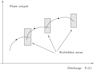
Figure 1: The generating domain of the plant $i$ is non-continuous

Figure 2: The domain defined by the constraints $\left(V_{i}(t)-V_{i}^{\mbox{\small max}}\right)D_{i}(t)=0$ is nonconvex

The numerical tests, hereafter outlined, use the current EDF regional modelling. Concerning the generating constraints ${\cal T}^{\mbox{\small ad}}_{i}$ :

• only a finite number of values is allowed for the discharge $T_{i}(t)$ (See Figure 4),

• there is a minimum delay between two variations of the discharge. Moreover, these variations have to be smooth.

The cost function $c_{i}(.,t)$ is a piecewiselinear function of the discharge and $C^{\mbox{\small end}}_{i}(V_{i}(H),H)$ is a linear function of the final content :

$$C^{\mbox{\small end}}_{i}(V_{i}(H),H)=c_{i}^{\mbox{\small wat}}\left(V_{i}(H)-V_{i}(0)\right)\enspace.$$

This modelling allows us to compare decomposition methods to the current EDF process. Nevertheless, the decomposition methods framework hereafter presented, could indeed be applied to more general modelling

3 Resolution Methods

In order to present the coordination-decomposition methods we use, we will consider the following problem:

$$\min_{u\in{\cal U}^{\mbox{\small ad}}}J(u)\enspace,\enspace\mbox{subject to:}\enspace\Theta(u)=0\enspace,$$ (9)

where ${\cal U}^{\mbox{\small ad}}$ is a closed set of a vector space ${\cal U}$, $J:{\cal U}\rightarrow{\mathbb{R}}$ and $\Theta:{\cal U}\rightarrow{\cal C}$ an affine function from ${\cal U}$ to the vectorial space ${\cal C}$. To allow decomposition, we also assume :

$${\cal U}=\prod_{i\in I}{\cal U}_{i}\enspace,\enspace{\cal U}^{\mbox{\small ad}}=\prod_{i\in I}{\cal U}^{\mbox{\small ad}}_{i}\enspace,$$

$$\forall u\in{\cal U}^{\mbox{\small ad}}\enspace:\enspace J(u)=\sum_{i\in I}J_{i}(u_{i})\enspace,$$

where $I$ is a finite set, ${\cal U}^{\mbox{\small ad}}_{i}\subset{\cal U}_{i}$ and $J_{i}:{\cal U}_{i}\rightarrow{\mathbb{R}}$.

3.1 Today’s resolution method

First of all, the convexified problem (problem (1), without constraints (7) and (8)) is solved by linear programming. Secondly, following the course of the river, for every plant, a feasible schedule is processed. In this aim, taking into account all the generating constraints, discharge is computed by minimizing a mean-square distance to the solution of the convexified problem. These subproblems are solved by dynamic programming.

It may be noticed that this heuristic has a major drawback : it does not ensure that a feasible solution will be found. The inflows being given, a subproblem may have no solution.

3.2 Price decomposition

3.2.1 Theoretical background

Provided that the cost function is separable, the Uzawa algorithm [4] is certainly the most commonly used to achieve this type of decomposition. If we suppose $\Theta(u)=\sum_{i\in I}\Theta_{i}(u_{i})$,then, applied to the problem (1), this algorithm may be outlined as follows ($k$ iteration):

$$\forall i\in I\;:\;\displaystyle\min_{u_{i}\in{\cal U}^{\mbox{\small ad}}_{i}}J_{i}(u_{i})+{\langle p^{k},\Theta_{i}(u_{i})\rangle}\;\Rightarrow\;u^{k+1}_{i}$$

$$p^{k+1}=p^{k}+\varepsilon^{k}\Theta(u^{k+1})\hfill$$

Therefore, at each iteration the $i$-subsystem minimizes a balance (the Lagrangian) which takes into account its own cost function $J_{i}$ and a “revenue” ${\langle p^{k},\Theta_{i}(u_{i})\rangle}$, from its contribution to the satisfaction of the constraint $\Theta(u)=0$.

More formally, the Lagrangian related to (9) is defined over ${\cal U}\times{\cal C}$ as follows :

$$\forall(u,p)\enspace:\enspace L(u,p)\stackrel{{\scriptstyle\mbox{\small def}}}{{=}}J(u)+{\langle p,\Theta(u)\rangle}\enspace.$$ (10)

The above mentioned algorithm may be understood as maximizing the dual function:

$$\Psi:p\mapsto\min_{u\in U^{\mbox{\small ad}}}L(u,p)$$

by a gradient type algorithm.

If the function $J$ is not strictly convex, as in the hydro-problem we are dealing with, this dual function is not differentiable. Consequently, to ensure the convergence, a sub-gradient algorithm must be used to maximize $\Psi$. The sequence $(\varepsilon^{k})_{k\in{\mathbb{N}}}$ must then be chosen as a sequence of type $\sigma$ (i.e. $\sum_{k=0}^{k=+\infty}\varepsilon^{k}=+\infty$ and $\sum_{k=0}^{k=+\infty}\left(\varepsilon^{k}\right)^{2}<+\infty$). The convergence is necessarily slow.

Nevertheless, the non-differentiability of the dual function is not the main difficulty. In this case, to find a price $p^{*}$ which maximizes the dual function $\Psi$ is not enough : for $p=p^{*}$, the primal minimization of the Lagrangian will not necessarily give a solution of (9) [5]. In practise, a “small” variation of the “prices” leads to a large variation of the primal variables. The primal variables “switch” from one value to another and never satisfy the coupling constraints. To our mind, these theoretical difficulties explain to a large extent the bad reputation that these dual methods have in terms of convergence.

However, Augmented Lagrangian can be used to reduce these difficulties. The Augmented Lagrangian $L_{c}$ related to the problem (9) is defined over ${\cal U}\times{\cal C}$ as follows :

$$\forall(u,p)\,:\,L_{c}(u,p)\stackrel{{\scriptstyle\mbox{\small def}}}{{=}}L(u,p)+{c\over 2}\|\Theta(u)\|^{2}$$ (11)

In the convex case, the saddle-points of this Lagrangian are the same as those of $L$ [6]. Then, the dual function $\Psi_{c}$ related to $L_{c}$ is differentiable [7]. Furthermore, solving $\min_{u\in U^{\mbox{\small ad}}}L_{c}(u,p^{*})$ where $p^{*}$ is a maximum of the dual function necessarily yields a solution of (9).

At first sight, this Augmented Lagrangian technique has a major drawback with regards to decomposition : it introduces non-separable terms ${c\over 2}\|\Theta(u)\|^{2}$. But, this difficulty can be overcome by linearizing the non-separable terms at each iteration [6]. This strategy leads to considering the following algorithm (algorithm A) (iteration $k+1$):

• for all $i\in I$, $u^{k+1}_{i}$ is computed by solving :

  $$\min_{u_{i}\in{\cal U}^{\mbox{\small ad}}_{i}}\left(J_{i}(u_{i})+\left\langle\pi^{k},\Theta_{i}(u_{i})\right\rangle+{b\over 2}\|u_{i}-u_{i}^{k}\|^{2}\right)\enspace,$$

• $p^{k+1}=p^{k}+\varepsilon\Theta(u^{k+1})$,

with $b\in{\mathbb{R}}^{+*}$ and $\pi^{k}=p^{k}+c\Theta(u^{k})$.

In the convex case, even if the cost function $J$ is not strictly convex, the convergence of this algorithm towards a saddle point of $L$ has been proven provided that $0<\varepsilon<2c$ and $c\tau^{2}<b$, where $\tau$ is the Lipschitz constant of $\Theta$ [6].

This algorithm has been shown to be particularly efficient in dealing with classical hydro-thermal generation scheduling problems [8], [5].

3.2.2 Application to the hydro-scheduling

problem In the problem (1), two types of constraints have to be handled:

• state constraints — the volumes bounds: $V_{i}(t)\in[V_{i}^{\mbox{\small min}},V_{i}^{\mbox{\small max}}]$ —,

• logical constraints concerning the controls which can be rather complex — $T\in{\cal T}^{\mbox{\small ad}}$ — .

Suppose that dynamic constraints (7) do not have to be dealt with. It would not be necessary to handle these two types of constraints simultaneously and the decomposition of (1) in simple subproblems would be allowed.

This remark led us to dualize dynamic constraints (7). Then, the application of the Algorithm A to (1) results, at the $k+1$ iteration, in the following steps:

• for all $i\in{\cal I}$, resolution of:

  $$\displaystyle\displaystyle\min_{T_{i}([0,H[)}\displaystyle\sum_{t\in[0,H[}\left\{-c_{i}(T_{i}(t),t)+{b\over 2}(T_{i}(t)-T^{k}_{i}(t))^{2}\enspace\enspace\right.$$

  $$\mbox{}+\left.\left(\pi^{k,k}_{i}(t)-\pi^{k,k}_{{{\mbox{\small av}(i)}}}(t+\delta_{{{\mbox{\small av}(i)}}\leftarrow i})\right)T_{i}(t)\right\}$$

  $$\mbox{s.t.\hskip 1.42271pt:}\enspace\enspace T_{i}([0,H[)\in{\cal T}^{\mbox{\small ad}}_{i}$$

  yields ${T}^{k+1}_{i}([0,H[)$,

• for all $i\in{\cal I}$ and $t\in[0,H[$, resolution of:

  $$\displaystyle\displaystyle\min_{{D}_{i}(t),{V}_{i}(t)}\displaystyle\left\{-C^{\mbox{\small end}}_{i}(V_{i}(t),t)\right.$$

  $$\mbox{}+\displaystyle\left(\pi^{k,k+1}_{i}(t)-\pi_{{\mbox{\small av}(i)}}^{k,k+1}(t+\delta_{{{\mbox{\small av}(i)}}\leftarrow i})\right)D_{i}(t)$$

  $$\mbox{}+\displaystyle{b\over 2}({D}_{i}(t)-{D}^{k}_{i}(t))^{2}+{b\over 2}({V}_{i}(t)-{V}^{k}_{i}(t))^{2}$$

  $$\left.\mbox{}+\displaystyle\left(\pi^{k,k+1}_{i}(t-1)-\pi^{k,k+1}_{i}(t)\right)V_{i}(t)\right\}$$

  subject to:

  $$V_{i}(t)\in[V_{i}^{\mbox{\small min}},V_{i}^{\mbox{\small max}}]\,,\quad D_{i}(t)\in[0,D_{i}^{\mbox{\small max}}]\,,$$

  $$\left(V_{i}(t)-V_{i}^{\mbox{\small max}}\right)D_{i}(t)=0\,,$$

  yields $\displaystyle({V}^{k+1}_{i}(t),{D}^{k+1}_{i}(t))$,

• for all $i\in{\cal I}$ and for all $t\in[0,H[$ the dual variables $p_{i}(t)$ are updated as follows:

  $$p^{k+1}_{i}(t)=p^{k}_{i}(t)+cH_{i}^{k+1,k+1}(t)$$

where:

• $c>0$ and $b>0$,

• $\forall i\in{\cal I}\,\;\forall t\in[0,H[~{}:$

  $$\displaystyle H_{i}^{k_{1},k_{2}}(t)\stackrel{{\scriptstyle\mbox{\small def}}}{{=}}V^{k_{1}}_{i}(t+1)-V^{k_{1}}_{i}(t)+D^{k_{1}}_{i}(t)$$

  $$\mbox{}+T^{k_{2}}_{i}(t)-A^{*}_{i}(t)-\sum_{j\in\Gamma^{T}_{i}}[D^{k_{1}}_{j}+T^{k_{2}}_{j}](t_{i\leftarrow j})\;,$$

  $$\displaystyle\pi^{k_{1},k_{2}}_{i}(t)\stackrel{{\scriptstyle\mbox{\small def}}}{{=}}p^{k_{1}}_{i}(t)+cH_{i}^{k_{1},k_{2}}(t)\enspace,$$

• $\forall t\in[0,H[\,:\,C^{\mbox{\small end}}_{i}(V_{i}(t),t)=0$.

At each iteration, a dynamic subproblem related to each plant (• ‣ 3.2.2) is solved. This subproblem handles mixed integer constraints concerning the plant discharge but no state constraints. It is solved by dynamic programming.

The problems (• ‣ 3.2.2) are very small and do not present any difficulties: only two real variables are optimized. Therefore, the subproblem resolutions that this algorithm requires, turn out to be quite simple.

Nevertheless, this is explained by the dualization of the most important constraints of the problem (1): the dynamic constraints. It may seem dubious, considering the mixed-integer constraints which have to be handled, that this dual method should achieve a feasible solution of (1).

To explain the numerical result which will be outlined further, it may be emphasized that this algorithm has been implemented in the following way:

• First of all, the “convexified” problem is solved using the price decomposition algorithm we have already described. In this case, the convexity assumptions being met, convergence is theoretically ensured and is obtained in practise. This first step yields a very good initial value of the dual variables $p_{i}(t)$.

• Then, every hundred iterations, until a feasible solution is reached, parameters are modified as follows:

  • the minimal bounds on the volumes $V_{i}^{\min}$ are slightly increased,

  • the value of parameter $c$ of the Augmented Lagrangian is multiplied (by $3$).

  Even if it has not been explained theoretically, this progressive increasing of parameter $c$ turns out to be a very efficient method for obtaining feasible solutions.

3.3 Interaction Prediction Principle

The second decomposition technique we consider lies on a simultaneous partitioning of variables and constraints. Every subproblem updates a set of variables handling a part of the constraints. Prices remunerate the sharing in the satisfaction of the constraints which are not coped with. Hence, this approach may be considered as mixing the price and resources decomposition techniques.

3.3.1 Theoretical Background

Takahara algorithm:

Consider problem (9). Suppose that $\Theta=\prod_{i=1}^{n}\Theta_{i}$ where: for all $i\in I$ : $\Theta_{i}:U\rightarrow{\cal C}_{i}$ and ${\cal C}=\prod_{i=1}^{n}{\cal C}_{i}$.

At the iteration $k$, Takahara algorithm [9], [10] substitutes to (1) a sequence of subproblems (14):

$$\begin{array}[]{l}\displaystyle\min_{u_{i}\in{\cal U}^{\mbox{\small ad}}_{i}}J_{i}(u_{i})+\sum_{j\neq i}{\langle p_{j}^{k},{\Theta}_{j}(u_{i},u_{-i}^{k})\rangle}\\ {{\displaystyle\Theta}_{i}(u_{i},u_{-i}^{k})=0}\end{array}$$ (14)

where $(u_{i},u_{-i}^{k})$ denotes the vector whose components are equal to those of $u^{k}$ except $u_{i}$.

Resolution of each (14) yields a primal solution $u_{i}^{k+1}$ and dual variables ($p_{i}^{k+1}$) related to the local constraint $\Theta_{i}(u_{i},u_{-i}^{k})=0$. $(p_{j}^{k})_{j\neq i}$ denote the dual variables that have been “predicted” by the other subproblems at step $k$. They are used to remunerate the participation of problem $i$ to the other constraints.

A primal-dual relaxation algorithm:

To explain the nature of this algorithm, let us assume that $J$ is differentiable and ${\cal U}^{\mbox{\small ad}}={\cal U}$. Then, Kuhn and Tucker necessary optimality conditions related to (1) may be written as follows:

$$\left\{\begin{array}[]{l}\forall i\in I\;:\;J^{{}^{\prime}}_{i}(u_{i})+\left(\Theta^{\prime}_{u_{i}}\right)^{*}p=0\enspace,\\ {\Theta}(u)=0\enspace.\end{array}\right.$$ (15)

Furthermore, if $(u^{k+1}_{i},p^{k+1}_{i})$ is a (primal-dual) solution of (14) then:

$$\left\{\begin{array}[]{l}J^{{}^{\prime}}_{i}(u_{i}^{k+1})+\sum_{j\neq i}\left(\Theta^{\prime}_{j,u_{i}}\right)^{*}p^{k}_{j}+\left(\Theta^{\prime}_{i,u_{i}}\right)^{*}p^{k+1}_{i}=0\enspace,\\ \Theta_{i}{(u_{i}^{k+1},u_{-i}^{k})}=0\enspace.\end{array}\right.$$

Consequently, the Takahara algorithm appears to be a primal-dual relaxation algorithm applied to the resolution of (15).

Find a saddle-point of the Augmented Lagrangian:

The algorithm we apply to the hydro-problem is built up in this way. However, this primal-dual relaxation framework is not used to find a saddle-point of $L$ but a saddle-point of the Augmented Lagrangian $L_{c}$ (11).

With the notation introduced above, at iteration $k$, it leads to solving the following subproblems:

$$\begin{array}[]{l}\displaystyle\min_{u_{i}\in{\cal U}^{\mbox{\small ad}}_{i}}\left(\begin{array}[]{c}J_{i}(u_{i})+\sum_{j\neq i}{\langle p_{j}^{k},{\Theta}_{j}(u_{i},u_{-i}^{k})\rangle}\\ +{c\over 2}\|{\Theta}(u_{i},u_{-i}^{k})\|^{2}\end{array}\right)\\ {{\displaystyle\Theta}_{i}(u_{i},u_{-i}^{k})=0}\end{array}$$ (20)

Although we will not present hereafter a comparative test on this purpose, it may be pointed out that, applied to the hydro-problem, (20) turns out to be more efficient than (14).

3.3.2 Application to the hydro-problem

In order to apply this algorithm, we first reformulate the hydro-problem (9). Variables $A_{i}^{+}(t)$ representing the global inflows of each reservoir are introduced:

$$A_{i}^{+}(t)-A_{i}^{*}(t)-\sum_{j\in\Gamma^{T}_{i}}[D_{j}+T_{j}](t_{i\leftarrow j})=0\enspace.$$ (21)

With this definition, the constraint

$$\displaystyle V_{i}(t+1)\,=\,V_{i}(t)+A_{i}^{+}(t)-D_{i}(t)-T_{i}(t)\enspace,$$ (22)

appears to be equivalent to the dynamic constraints (7).

To split (1) into a sequence of subproblems, each related to a plant, algorithm (20) is then applied in the following way:

• vector $\left(A_{i}^{+}(t),T_{i}(t),D_{i}(t)\right)_{t\in[0,H[}$ is $u_{i}$,

• constraints (21) are considered as being the coupling constraints $\Theta$,

• constraints (22), (7), (7) and (8) define the domain ${\cal U}^{\mbox{\small ad}}$ of (9),

• $J_{i}(u_{i})=\displaystyle\sum_{t\in[0,H[}-c_{i}(T_{i}(t),t)-C^{\mbox{\small end}}_{i}(V_{i}(H),H)$.

With these choices, the algorithm (20) leads to solving, at iteration $k+1$, the following subproblems (Algorithm B):

$$\displaystyle\min_{T_{i}\in{\cal T}^{\mbox{\small ad}}_{i}}\sum_{t\in[0,H[}\left\{-c_{i}(T_{i}(t),t)-C^{\mbox{\small end}}_{i}(V_{i}(H),H)\right.$$

$$\mbox{}-p_{{\mbox{\small av}(i)}}^{k}(t)\,[T_{i}+D_{i}](t_{{\mbox{\small av}(i)}\leftarrow i})$$

$$\left.\mbox{}+{c\over 2}\|DT_{i}^{k}(t)-[D_{i}+T_{i}](t_{{\mbox{\small av}(i)}\leftarrow i})\|^{2}\right\}$$

$$\displaystyle\mbox{s.t.: }V_{i}(t+1)\,=\,V_{i}(t)-D_{i}(t)-T_{i}(t)+A^{*}_{i}(t)$$

$$\mbox{}+\sum_{j\in\Gamma^{T}_{i}}\left[D^{k}_{j}+T^{k}_{j}\right](t_{i\leftarrow j})$$

    (7), (7) and (8)  .

with: $$\quad DT_{i}^{k}(t)\,=\,A_{{\mbox{\small av}(i)}}^{+}(t)^{k}-A_{{\mbox{\small av}(i)}}^{*}(t)^{k}$$

$$\displaystyle\qquad-\sum_{j\in\Gamma^{T}_{{\mbox{\small av}(i)}}-\{i\}}[D^{k}_{j}+T^{k}_{j}](t_{{\mbox{\small av}(i)}\leftarrow j})\enspace.$$

A sequential version of this algorithm has been implemented. Following the course of the river, each subproblem is solved taking into account the results of the current iteration (for the upstream informations) and of the preceding iteration (for the downstream). In this context, $DT_{i}^{k}(t)$ is necessarily equal to $[D^{k}_{i}+T^{k}_{i}](t_{{\mbox{\small av}(i)}\leftarrow i})$ and at iteration $k+1$, the subproblem related to the plant $i$ may be written as follows:

$$\displaystyle\min_{T_{i}\in{\cal T}^{\mbox{\small ad}}_{i}}\sum_{t\in[0,H[}\left\{-c_{i}(T_{i}(t),t)-C^{\mbox{\small end}}_{i}(V_{i}(H),H)\right.$$

$$\mbox{}-p_{{\mbox{\small av}(i)}}^{k}(t)[T_{i}+D_{i}](t_{{\mbox{\small av}(i)}\leftarrow i})$$

$$\left.\mbox{}+{c\over 2}{\|[D_{i}+T_{i}]^{k}(t_{{\mbox{\small av}(i)}\leftarrow i})-[D_{i}+T_{i}](t_{{\mbox{\small av}(i)}\leftarrow i})\|}^{2}\right\}$$

$$\mbox{s.t.: }V_{i}(t+1)\,=\,V_{i}(t)-D_{i}(t)-T_{i}(t)+A^{*}_{i}(t)$$

$$\mbox{}\displaystyle\hskip 14.22636pt+\sum_{j\in\Gamma^{T}_{i}}[D^{k+1}_{j}+T^{k+1}_{j}](t_{i\leftarrow j})$$

$$\mbox{\hskip 11.38092pt(\ref{exclus}), (\ref{borne}) and (\ref{turbi})}\enspace.$$

Therefore, handling its generating constraints and taking into account the discharge the upstream plants have computed, each plant optimizes its schedule. The dual variable $p_{{\mbox{\small av}(i)}}^{k}$ may be understood as being the price the downstream reservoir “would pay” its water inflows. Quadratic terms introduced by the Augmented Lagrangian appear to be a type of “brake” avoiding the oscillations of the algorithm.

It may also be noticed the subproblems (3.3.2) turn out to have exactly the same structure as the local problems of the heuristic process currently in use (See Today’s methods). Therefore, from a practical point of view, Algorithm B appears to be an extension of this heuristic method. Moreover, providing there is no pumping unit, this sequential version generally yields a feasible solution at the first iteration.

4 Numerical Tests

4.1 A hydraulic valleys sample

A sample of hydraulic valleys has been chosen so as to point out, as well as possible, the main resolution difficulties.

Size and topology: The hydraulic valley is illustrated in Figure 3. It contains six reservoirs and to each reservoir $R_{i}$ is related a plant $U_{i}$.

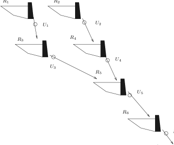
Figure 3: Hydraulic test valley

Volume bounds: The upstream reservoirs 1 and 2 are supposed to have a large storage capacity: on a daily scale, no volume constraints have to be coped with. The other reservoirs are characterized by the ratio of their storage and hourly-discharge capacities. Three sets of storage/discharge ratios are considered:

• $1\mbox{ h }30$ for reservoirs $2$ and $4$, $5\mbox{h}$ for reservoirs $5$ and $6$,

• $0\mbox{ h }30$ for reservoirs $2$ and $4$, $3\mbox{h}$ for reservoirs $5$ and $6$,

• $5\mbox{ h }$ for reservoirs $2$ and $4$, $15\mbox{h}$ for reservoirs $5$ and $6$.

There are no natural inflows.

Cost function: The generation “revenue” $c_{i}(T_{i}(t),t)$ is assumed to be a linear function of the discharge (i.e. $c_{i}(T_{i}(t),t)=p^{\mbox{\small gen}}(t)T_{i}(t)$). Three sequences $(p^{\mbox{\small gen}}(t))_{t\in[0,H[}$ are considered (in Francs per MWh):

• The first ranges from $99$ to $101$. It “switches” from one value to another every $4$ hours. This price vector enables the numerical accuracy of the algorithms to be tested.

• The second remains at $100$ over the whole period except four hours during which it rises up to $500$. Such a choice enables the spinning reserve over a four hour period to be computed. The ability to optimize feasible controls in real-time and in case of emergency is also measured in this way. From a numerical point of view, it is in this case that constraints (7) and (7) are actually active.

• Every four hours, the third switches between $80$ and $120$.

Discharge Constraints: For each plant $U_{i}$, the discharge belongs to a discrete set of values (See Figure 4).

The minimum delay between two discharge variations may be $0$ (D1), $1$ (D2) or $4$ (D3) hours.

The (D4), (D5) and (D6) are deduced from (D1), (D2) or (D3) by supposing the plants $3$ and $4$ are out-of-order (have no discharge capacity).

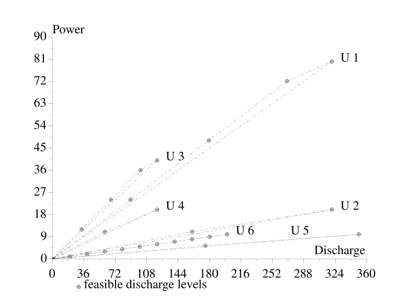
Figure 4: The generation is a piecewise linear function of the discharge

Crossing these factors, it is a $56$ valleys sample which is built up. It may be noticed the non-continuities in the discharge domain are actually sizeable. For the V2 storage/discharge ratio, the choice of a discharge level rather than another modify the hourly discharge by about half the storage capacity !

4.2 Numerical results

The two decomposition algorithms and the process currently in use at EDF have been compared over this sample of valleys.

The “scores” are computed in the following way. For each tested algorithm and each sample of valley, the maximum gain $\sum_{t\in[0,H[}c_{i}(T_{i}(t),t)+C^{\mbox{\small end}}_{i}(V_{i}(H),H)$ obtained by a feasible solution along the iterations is recorded. If no feasible solution is found, this gain is considered to be zero: because there are no natural inflows, a zero discharge solution is possible and its gain is zero.

Then, relative gains (or “scores”) are computed by dividing these gains by those of the best solutions achieved by one of the three processes.

	Alg.	Alg.	Alg.	Alg.
	A	B	C	L
P1 (m.s.)	83.2 %	83.8 %	62.3 %	186 %
P1 (a.f.)	100 %	100%	72 %	0 %
P2 (m.s.)	99.4 %	99.9 %	99.7 %	100 %
P2 (a.f.)	100 %	100%	100 %	0 %
P3 (m.s.)	97.1%	90.4 %	90.8 %	109.2 %
P3 (a.f.)	100%	100 %	100 %	0 %
M (m.s.)	93.2 %	91.4 %	84.3 %	131.8 %
M (a.f.)	100%	100 %	91 %	0 %

Table 1: Mean scores (m.s.) and average feasibility (a.f.) for each “prices system” (P1, P2, P3) and for the whole sample M.

Table 1 gives mean scores (m.s.) and feasibility average rates (f.a.) for the three types of “generation prices” which have been considered (P1, P2, P3) and for the whole sample (M). In every case, the two decomposition methods yield feasible solutions. Considering how significant the non-continuities are it is a remarkable achievement.

In spite of the efficiency of the heuristic process which is currently in use at EDF (Algorithm C) — in more than $90$ percent of the (difficult) cases we have selected, feasible solutions are reached — these methods thus represent a real improvement.

Furthermore, if constraints (8) and (7) are not handled, problem (1) is convex. It can be solved by linear programming. The mean “score” of the non feasible solutions obtained in this way are also indicated in Table 1 (Algorithm L). One may consider that about twenty percents of the current cost of the nonconvexities in the (1) modelling are saved thanks to these decomposition methods.

What CPU time ?

For the valley of six reservoirs we consider, the heuristic resolution today in use at EDF takes about $10$ seconds on a SUN $4/40$. One half of this time is dedicated to the linear optimization the other is used by the six dynamic programming resolution which are necessary to find a solution.

For the prediction strategy, the results presented above correspond to $25$ iterations. Each of these having the same complexity as the heuristic research of a feasible solution, the CPU time required is more or less $2$ minutes.

Our implementation of the price decomposition method uses about $1200$ iterations. This number may seem important. Nevertheless, the subproblems are particularly simple and, for the six reservoirs valleys, CPU time does not exceed $2$ minutes.

If these times are not huge, they multiply by ten CPU times of the current process. Therefore, work is currently undertaken to reduce these CPU times. To our mind, on average, they should be divided by about $5$ in the final implementation by:

• improving the software design,

• avoiding to solve each subproblem at each iteration.

What is the best method ?

We have already noticed the average “score” (M) of the price decomposition is $93.2\%$, the prediction one being $91.4\%$. Should the prediction method be rejected ? We have not made such a choice for two reasons:

• contrary to the price decomposition strategy, the relaxation algorithm generally yields, from the first iterations, a feasible solution,

• if, on average, price decomposition method reaches the best solutions, it does not in every case. Furthermore, if one choose the best of the two solutions these methods yield, it would not be $93.2\%$ or $91.4\%$ but a score of $100\%$ which would be reached. In fact, the tools we are currently developing, on the basis of these first tests, will try to take advantage of each of these methods. By experimentations, we aim at establishing rules which, after considering the characteristics of the valley, choose the best of the two algorithms.

5 Conclusion

Over the $56$ numerical tests which have been carried out, in spite of the mixed-integer constraints which are handled, the decomposition methods considered allow a feasible solution to be systematically found. Moreover, compared to the two-step process currently in use at EDF, those methods yield sizeable savings.

For these reasons, these methods will be used to design new regional level software at Electricité de France.

Furthermore, by proving the robustness of these decomposition approaches, these tests open up new fields of research. A global optimization of generation schedules of several hydraulic valleys, handling coupling constraints (demand constraints), could be achieved in this way.

References

- [1] Maurras J.F., “Optimization of the Flow through Networks with Gains,” Mathematical Programming, Vol. 3, 2, pp. 135-144, 1972.
- [2] Merlin A., Lauzanne B., Maurras J.-F., Auge J. and Ziglioli M., “Optimization of Short-trem Scheduling of EDF Hydraulic Valleys with Coupling Constraints: the OVIDE Model”, Proc. PSCC, pp. 345-354, 1981.
- [3] Ea K., Monti M., Jouve M., Kiener A. “Daily Operational Planning of the EDF Plant Mix: The Octave Model optimizes Lake Plant Discharges”, Proc. PSCC pp. 175-181, 1987.
- [4] Arrow K., Hurwicz L., Uzawa H., “Studies in Linear and Nonlinear Programming,” Standford University Press, Stanford, USA.
- [5] Batut J., Renaud A., “Daily Generation Scheduling with Transmission Constraints : A New Class of Algorithms,” IEEE Transactions on Power Systems, Vol.7, 3, pp. 982-989, August 1992.
- [6] Cohen G., Zhu D.L., “Decomposition Coordination Methods in Large Scale Optimization Problems. The Nondifferentiable Case and the Use of Augmented Lagrangian”, In: J.B. Cruz, Ed. Advances in Large Scale Systems Theory and Applications, Vol. I., JAI Press, Greenwich, Connecticut, 1984.
- [7] Rockafellar R.T., “A Dual Approach to Solving Nonlinear Programming Problems by Unconstrained Optimization”, Mathematical Programming, 5 , pp. 354-373, 1973.
- [8] Batut J., Renaud A., Sandrin P., “A New Software for Generation Rescheduling in the future EDF national control center,” Proc. PSCC Graz,1990.
-
[9]
Takahara Y., Multilevel Approach to Dynamic
Optimization, Report SRC-50-C-64-18, Case
Western Reserve University, Cleveland, Ohio,
1964. -
[10]
Cohen G., Miara B., “Optimization with an
Auxiliary Constraint and Decomposition”, SIAM J. of Control and Optimization, Vol. 28, No. 1, pp. 137-157, January 1990.