A General Compressive Sensing Construct using Density Evolution

Abstract

This paper proposes a general framework to design a sparse sensing matrix $\mathbf{A}\in\mathbb{R}^{m\times n}$, for a linear measurement system $\mathbf{y}=\mathbf{Ax}^{\natural}+\mathbf{w}$, where $\mathbf{y}\in\mathbb{R}^{m}$, $\mathbf{x}^{\natural}\in\mathbb{R}^{n}$, and $\mathbf{w}\in\mathbb{R}^{m}$ denote the measurements, the signal with certain structures, and the measurement noise, respectively. By viewing the signal reconstruction from the measurements as a message passing algorithm over a graphical model, we leverage tools from coding theory in the design of low density parity check codes, namely the density evolution technique, and provide a framework for the design of matrix $\mathbf{A}$. Two design schemes for the sensing matrix, namely, $(i)$ a regular sensing and $(ii)$ a preferential sensing, are proposed and are incorporated into a single framework. As an illustration, we consider the $\ell_{1}$ regularizer, which corresponds to Lasso for both of the schemes. In the regular sensing scenario, our framework can reproduce the classical result of Lasso, i.e., $m\geq c_{0}k\log(n/k)$ after a proper distribution approximation, where $c_{0}>0$ is some fixed constant. In the preferential sensing scenario, we consider the case in which the whole signal is divided into two disjoint parts, namely, high-priority part $\mathbf{x}^{\natural}_{H}$ and low-priority part $\mathbf{x}^{\natural}_{L}$. Then, by formulating the sensing system design as a bi-convex optimization problem, we obtain a sensing matrix $\mathbf{A}$ which provides a preferential treatment for $\mathbf{x}^{\natural}_{H}$. Numerical experiments with both synthetic data and real-world data suggest a significant reduction of the $\ell_{2}$ error in the high-priority part $\mathbf{x}^{\natural}_{H}$ and a slight reduction of the $\ell_{2}$ error in the whole signal $\mathbf{x}^{\natural}$. Apart from the sparse signal with $\ell_{1}$ regularizer, our framework is flexible and capable of adapting the design of the sensing matrix $\mathbf{A}$ to a signal $\mathbf{x}^{\natural}$ with other underlying structures.

Introduction

This paper considers a linear sensing relation as

$$\mathbf{y}=\mathbf{A}\mathbf{x}^{\natural}+\mathbf{w},$$ (1.1)

where $\mathbf{y}\in\mathbb{R}^{m}$ denotes the measurements, $\mathbf{A}\in\mathbb{R}^{m\times n}$ is the sensing matrix, $\mathbf{x}^{\natural}\in\mathbb{R}^{n}$ is the signal to be reconstructed, and $\mathbf{w}\in\mathbb{R}^{m}$ is the measurement noise with iid Gaussian distribution $\mathsf{N}(0,\sigma^{2})$. To reconstruct $\mathbf{x}^{\natural}$ from $\mathbf{y}$, one widely used method is the regularized M-estimator

$$\widehat{\mathbf{x}}=\textup{argmin}_{\mathbf{x}\in\mathbb{R}^{n}}~{}\frac{1}{2\sigma^{2}}{\left\|\mathbf{y}-\mathbf{A}\mathbf{x}\right\|}_{2}^{2}+f(\mathbf{x}),$$ (1.2)

where $f(\cdot)$ is the regularizer used to enforce a desired structure for $\widehat{\mathbf{x}}$. To ensure reliable recovery of $\mathbf{x}^{\natural}$, sensing matrix $\mathbf{A}$ needs to satisfy certain conditions, e.g., the incoherence in Donoho et al., (2005), RIP in Candes et al., (2006); Candès et al., (2006), the neighborhood stability in Meinshausen et al., (2006), irrespresentable condition in Zhao & Yu, (2006), etc. Notice that all the above works treat each entry of $\mathbf{x}^{\natural}$ equally. However, in certain applications, entries of $\mathbf{x}^{\natural}$ may have unequal importance from the recovery perspective. One practical application is the image compression, i.e., JPEG compression, where coefficients corresponding to the high-frequency part are more critical than the rest of coefficients.

In this work, we focus on the sparse sensing matrix $\mathbf{A}$. Leveraging tools from coding theory, namely, density evolution (DE), we propose a heuristic but general design framework of $\mathbf{A}$ to meet the requirements of the signal reconstruction such as placing more importance on the accuracy of a certain components of the signal. At the core of our work is the application of DE in message passing (MP) algorithm, which is also referred to as belief propagation, or sum-product, or min-sum algorithm. These different names are due to its broad spectrum of applications and its constant rediscovery in different fields. In physics, this algorithm existed no later than $1935$, when Bethe used a free-energy functional to approximate the partition function (cf. Mezard & Montanari, (2009)). In the probabilistic inference, Pearl developed it in $1988$ for acyclic Bayesian networks and showed it leads to the exact inference Pearl, (2014). The most interesting thing is its discovery in the coding theory. In early 1960s, Gallager proposed sum-product algorithm to decode low density parity check (LDPC) codes over graphs Gallager, (1962). However, Gallagher work was almost forgotten and was rediscovered again in 90s Berrou & Glavieux, (1996); McEliece et al., (1998). Later Richardson & Urbanke, (2001) equipped it with DE and used it for the design of LDPC codes for capacity achieving over certain channels.

When narrowing down to the compressed sensing (CS), MP has been widely used for signal reconstruction Sarvotham et al., (2006a); Zhang & Pfister, (2012); Kudekar & Pfister, (2010); Eftekhari et al., (2012); Krzakala et al., (2012b, a); Zdeborová & Krzakala, (2016); Donoho et al., (2009); Maleki, (2010) and analyzing the performance under some specific sensing matrices. The following briefly discusses the related work in the sensing matrix.

Related work. In the context of the sparse sensing matrix, the authors in Sarvotham et al., (2006b) first proposed a so-called sudocode construction technique and later presented a decoding algorithm based on the MP in Baron et al., (2009). In Chandar et al., (2010), the non-negative sparse signal $\mathbf{x}^{\natural}$ is considered under the binary sensing matrix. The work in Dimakis et al., (2012) linked the channel encoding with the CS and presented a deterministic way of constructing sensing matrix based on a high-girth LDPC code. In Luby & Mitzenmacher, (2005); Zhang & Pfister, (2012); Eftekhari et al., (2012), the authors considered the verification-based decoding and analyzed its performance with DE. In Kudekar & Pfister, (2010), the spatial coupling is first introduced into CS and is evaluated with the decoding scheme adapted from Luby & Mitzenmacher, (2005). However, all the above mentioned works focused on the noiseless setting, i.e., $\mathbf{w}=\mathbf{0}$ in (1.1). In Krzakala et al., (2012b, a); Zdeborová & Krzakala, (2016), the noisy measurement is considered. A sparse sensing matrix based on spatial coupling is analyzed in the large system limit with replica method and DE. They proved its recovery performance to be optimal when $m$ increases at the same rate of $n$, i.e., $m=O(n)$.

Moreover, in the context of a dense sensing matrix, the analytical tool switches from DE to state evolution (SE), which is first proposed in Donoho et al., (2009); Maleki, (2010). Together with SE comes the approximate message passing (AMP) decoding scheme. The empirical experiments suggest AMP has better scalability when compared with $\ell_{1}$ construction scheme without much scarifice in the performance. Additionally, an exact phase transition formula can be obtained from SE, which predicts the performance of AMP to a good extent. Later, Bayati & Montanari, (2011) provided a rigorous proof for the phase transition property by the conditioning technique from Erwin Bolthausen and Donoho & Montanari, (2016) extended AMP to general M-estimation.

Note that the above mentioned related works are not exhaustive due to their large volume. For a better understanding of the MP algorithm, the DE, and their application to the compressive sensing, we refer the interested readers to Mezard & Montanari, (2009); Montanari, (2012); Zdeborová & Krzakala, (2016). In addition to the work based on MP, there are other works based on LDPC codes or graphical models. Since they are not closely related to ours, we only mention their names without further discussion Xu & Hassibi, (2007a, b); Khajehnejad et al., (2009); Jafarpour et al., (2009); Lu et al., (2012); Zhang et al., (2015); Mousavi et al., (2017).

Contributions. Compared to the previous works exploiting MP Luby & Mitzenmacher, (2005); Zhang & Pfister, (2012); Eftekhari et al., (2012); Kudekar & Pfister, (2010); Krzakala et al., (2012b, a); Zdeborová & Krzakala, (2016); Donoho et al., (2009); Maleki, (2010), our focus is on the sensing matrix design rather than the decoding scheme, which is based on the M-estimator with regularizer. Exploiting the DE, we propose a universal framework which supports both the regular sensing and the preferential sensing for recovering the signal. Taking the sparse recovery with $\ell_{1}$ regularizer as an example, we list our contributions as follows.

• Regular Sensing. We consider the $k$-sparse signal $\mathbf{x}^{\natural}\in\mathbb{R}^{n}$ and associate it with a prior distribution such that each entry is zero with probability $1-k/n$. First we approximate this distribution with Laplacian prior by letting the probability mass near the origin point to be $1-k/n$. Afterwards, we can reproduce the classical results in CS, i.e., $m\geq c_{0}k\log n$.

• Preferential Sensing. We design the sensing matrix that would result in more accurate (or exact) recovery of the high-priority sub-block of the signal relative to the low-priority sub-block. Numerical experiments suggest our framework can $(i)$ reduce the error in the high-priority sub-block significantly; and $(ii)$ yet be able to reduce the error with regard to the whole signal modestly as well. Additionally, we emphasize that although we focus on two levels of priority in signal components in this work, we can easily extend the framework to the scenario where multiple levels of preferential treatment on the signal components are needed, by simply incorporating associated equations into the DE.

Organization. In Sec. 2, we formally state our problem and construct the graphical model. In Sec. 3, we focus on the regular sensing and propose the density evolution framework. In Sec. 4, the framework is further extended to the preferential sensing. Generalizations are presented in Sec. 5, simulation results are put in Sec. 6, and conclusions are drawn in Sec. 7.

Problem Description

We begin this section with a formal statement of our problem. Consider the linear measurement system

$$\mathbf{y}=\mathbf{A}\mathbf{x}^{\natural}+\mathbf{w},\vspace{-1mm}$$

where $\mathbf{y}\in\mathbb{R}^{m}$, $\mathbf{A}\in\mathbb{R}^{m\times n}$, $\mathbf{x}^{\natural}\in\mathbb{R}^{n}$, and $\mathbf{w}\in\mathbb{R}^{m}$, respectively, denote the observations, the sensing matrix, the signal, and the additive sensing noise with its $i$th entry $w_{i}\stackrel{{\scriptstyle\textup{i.i.d}}}{{\sim}}\mathsf{N}(0,\sigma^{2})$. We would like to recover $\mathbf{x}^{\natural}$ with the regularized M-estimator, which is written as

$$\widehat{\mathbf{x}}=\textup{argmin}_{\mathbf{x}}\frac{1}{2\sigma^{2}}{\left\|\mathbf{y}-\mathbf{A}\mathbf{x}\right\|}_{2}^{2}+f(\mathbf{x}),$$

where $f(\cdot)$ is the regularizer used to enforce certain underlying structure for signal $\widehat{\mathbf{x}}$. Our goal is to design a sparse sensing matrix $\mathbf{A}$ which provides preferential treatment for a sub-block of the signal $\mathbf{x}^{\natural}$. In other words, the objective is to have a sub-block of the signal to be recovered with lower probability of error when comparing with the rest of $\mathbf{x}^{\natural}$. Before we proceed, we list our two assumptions:

• Measurement system $\mathbf{A}$ is assumed to be sparse. Further, $\mathbf{A}$ is assumed to have entries with $\mathbb{E}A_{ij}=0$, and $A_{ij}\in\{0,\pm A^{-1/2}\}$, where an entry $A_{ij}=A^{-1/2}$ (or $-A^{1/2}$) implies a positive (negative) relation between the $i$th sensor and the $j$th signal component. Having zero as entry implies no relation.

• The regularizer $f(\mathbf{x})$ is assumed to be separable such that $f(\mathbf{x})=\sum_{i=1}^{n}f_{i}(x_{i})$. If it is not mentioned specifically, we assume all functions $f_{i}(\cdot)$ are the same.

First we transform (1.1) to a factor graph Richardson & Urbanke, (2008). Adopting the viewpoint of Bayesian reasoning, we can reinterpret M-estimator in (1.2) as the maximum a posteriori (MAP) estimator and rewrite it as

$$\widehat{x}=\textup{argmax}_{x}\exp\left(-\frac{{\left\|\mathbf{y}-\mathbf{A}\mathbf{x}\right\|}_{2}^{2}}{2\sigma^{2}}\right)\times\exp\left(-f(\mathbf{x})\right).\vspace{1mm}$$

The first term $\exp\left(-\frac{{\left\|\mathbf{y}-\mathbf{A}\mathbf{x}\right\|}_{2}^{2}}{2\sigma^{2}}\right)$ is viewed as the probability $\mathbb{P}(\mathbf{y}|\mathbf{x})$ while the second term $\exp(-f(\mathbf{x}))$ is regarded as the prior imposed on $\mathbf{x}$. Notice the term $e^{-f(\cdot)}$ may not necessarily be the true prior on $\mathbf{x}^{\natural}$.

As in Montanari, (2012), we associate (1.2) with a factor graph ${\cal G}=\left({\cal V},{\cal E}\right)$, where ${\cal V}$ denotes the node set and ${\cal E}$ is the edge set. First we discuss set ${\cal V}$, which consists of two types of nodes: variable nodes and check nodes. We represent each entry $x_{i}$ as a variable node $v_{i}$ and each entry $y_{a}$ as a check node $c_{a}$. Additionally, we construct a check node corresponds to each prior $e^{-f(x_{i})}$. Then we construct the edge set ${\cal E}$ by: $(i)$ placing an edge between the check node of the prior $e^{-f(x_{i})}$ and the variable node $v_{i}$, and $(ii)$ introducing an edge between the variable node $v_{i}$ and $c_{j}$ iff $A_{ij}$ is non-zero. Thus, the design of $\mathbf{A}$ is transformed to the problem of graph connectivity in ${\cal E}$. Before to proceed, we list the notations used in this work.

Notations. We denote $c,c^{{}^{\prime}},c_{0}>0$ as some fixed positive constants. For two arbitrary real numbers $a,b$, we denote $a\lesssim b$ when there exists some positive constant $c_{0}>0$ such that $a\leq c_{0}b$. Similarly, we define the notation $a\gtrsim b$. If $a\lesssim b$ and $a\gtrsim b$ hold simultaneously, we denote as $a\asymp b$. We have $a\propto b$ when $a$ is proportional to $b$. For two distributions $d_{1}$ and $d_{2}$, we denote $d_{1}\cong d_{2}$ if they are equal up to some normalization.

Sensing Matrix for Regular Sensing

With the aforementioned graphical model, we can view recovering $\mathbf{x}^{\natural}$ as an inference problem, which can be solved via the message-passing algorithm Richardson & Urbanke, (2008). Adopting the same notations as in Montanari, (2012) as shown in Fig. 1, we denote $m_{i\rightarrow a}^{(t)}$ as the message from the variable node $v_{i}$ to check node $c_{a}$ at the $t^{\mathsf{th}}$ round of iteration. Likewise, we denote $\widehat{m}_{a\rightarrow i}^{(t)}$ as the message from the check node $c_{a}$ to variable node $v_{i}$. Then message-passing algorithm is written as

$$m_{i\rightarrow a}^{(t+1)}(x_{i}) \cong e^{-f(x_{i})}\prod_{b\in\partial i\setminus a}\widehat{m}_{b\rightarrow i}^{(t)}(x_{i});$$ (3.1)

$$\widehat{m}_{a\rightarrow i}^{(t+1)}(x_{i}) \cong\int\prod_{j\in\partial a\setminus i}m_{j\rightarrow a}^{(t+1)}(x_{i})\cdot e^{-\frac{\left(y_{a}-\sum_{j=1}^{n}A_{aj}x_{j}\right)^{2}}{2\sigma^{2}}}dx_{j},$$ (3.2)

where $\partial i$ and $\partial a$ denote the neighbors connecting with $v_{i}$ and $c_{a}$, respectively, and the symbol $\cong$ refers to the equality up to the normalization. At the $t$th iteration, we recover $x_{i}$ by maximizing the posterior probability

$$\widehat{x}^{(t)}_{i}=\textup{argmax}_{x_{i}}\mathbb{P}(x_{i}|\mathbf{y})\approx\textup{argmax}_{x_{i}}e^{-f(x_{i})}\prod_{a\in\partial i}\widehat{m}_{a\rightarrow i}^{(t)}(x_{i}).$$ (3.3)

In the design of matrix $\mathbf{A}$, there are some general desirable properties that we wish to hold (specific requirements will be discussed later): $(i)$ a correct signal reconstruction under the noiseless setting; and $(ii)$ minimum number of measurements, or equivalently minimum $m$. Before proceeding, we first introduce the generating polynomials $\lambda(\alpha)=\sum_{i}\lambda_{i}\alpha^{i-1}$ and $\rho(\alpha)=\sum_{i}\rho_{i}\alpha^{i-1}$, which correspond to the degree distributions for variable nodes and check nodes, respectively. We denote the coefficient $\lambda_{i}$ as the fraction of variable nodes with degree $i$, and similarly we define $\rho_{i}$ for the check nodes. An illustration of the generating polynomials $\lambda(\alpha)$ and $\rho(\alpha)$ is shown in Fig. 2.

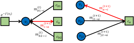
Figure 1: Illustration of the message-passing algorithm, where the square icons represent the check nodes while the circle icons represent the variable nodes.

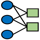
Figure 2: Illustration of the generating polynomials: $\lambda(\alpha)=\frac{1}{3}+\frac{2\alpha}{3}$ and $\rho(\alpha)=\frac{\alpha}{2}+\frac{\alpha^{2}}{2}$. The square icons represent the check nodes while the circle icons represent the variable nodes.

Density evolution

To design the matrix $\mathbf{A}$, we study the reconstruction of $\mathbf{x}^{\natural}$ from $\mathbf{y}$ via the convergence analysis of the message-passing over the factor graph. Due to the parsimonious setting of $\mathbf{A}$, we have ${\cal E}$ to be sparse and propose to borrow a tool known as density evolution (DE) Richardson et al., (2001); Richardson & Urbanke, (2008); Chung, (2000) that is already proven to be very powerful in analyzing the convergence in sparse graphs resulting from LDPC.

Basically, DE views $m_{i\rightarrow a}^{(t)}$ and $\widehat{m}_{a\rightarrow i}^{(t)}$ as RVs and tracks the changes of their probability distribution. When the message-passing algorithm converges, we would expect their distributions to become more concentrated. However, different from discrete RVs, continuous RVs $m_{i\rightarrow a}^{(t)}$ and $\widehat{m}_{a\rightarrow i}^{(t)}$ in our case require infinite bits for their precise representation in general, leading to complex formulas for DE. To handle such an issue, we approximate $m_{i\rightarrow a}^{(t)}$ and $\widehat{m}_{a\rightarrow i}^{(t)}$ as Gaussian RVs, i.e., $m_{i\rightarrow a}\sim\mathsf{N}(\mu_{i\rightarrow a},v_{i\rightarrow a})$ and $\widehat{m}_{a\rightarrow i}\sim\mathsf{N}(\widehat{\mu}_{a\rightarrow i},\widehat{v}_{a\rightarrow i})$, respectively. Since the Gaussian distribution is uniquely determined by its mean and variance, we will be able to reduce the DE to finite dimensions as in Chung, (2000); Krzakala et al., (2012b, a).

In our work, the DE tracks two quantities $E^{(t)}$ and $V^{(t)}$, which denote the deviation from the mean and average of the variance, respectively, and are defined as

$$E^{(t)} =\frac{1}{m\cdot n}\sum_{i=1}^{n}\sum_{a=1}^{m}\left(\mu_{i\rightarrow a}^{(t)}-x^{\natural}_{i}\right)^{2};$$

$$V^{(t)} =\frac{1}{m\cdot n}\sum_{i=1}^{n}\sum_{a=1}^{m}v_{i\rightarrow a}^{(t)}.\vspace{1mm}$$

Then we can show that the DE analysis yields

$$E^{(t+1)}=\mathbb{E}_{\textup{prior}(s)}\mathbb{E}_{z}\bigg{[}h_{\textup{mean}}\bigg{(} s+\sum_{i,j}\rho_{i}\lambda_{j}z\sqrt{\frac{i}{j}E^{(t)}+\frac{A\sigma^{2}}{j}};$$

$$\sum_{i,j}\rho_{i}\lambda_{j}\frac{A\sigma^{2}+iV^{(t)}}{j}\bigg{)}-s]^{2};$$ (3.4)

$$V^{(t+1)}=\mathbb{E}_{\textup{prior}(s)}\mathbb{E}_{z}h_{\textup{var}}\bigg{(} s+\sum_{i,j}\rho_{i}\lambda_{j}z\sqrt{\frac{i}{j}E^{(t)}+\frac{A\sigma^{2}}{j}};$$

$$\sum_{i,j}\rho_{i}\lambda_{j}\frac{A\sigma^{2}+iV^{(t)}}{j}\bigg{)},$$ (3.5)

where $\textup{prior}(\cdot)$ denotes the true prior on the entries of $\mathbf{x}^{\natural}$, and $z$ is a standard normal RV $\mathsf{N}(0,1)$. The functions $h_{\textup{mean}}(\cdot)$ and $h_{\textup{var}}(\cdot)$ are to approximate the mean $\mu_{i\rightarrow a}$ and variance $v_{i\rightarrow a}$, which are given by

$$h_{\textup{mean}}(\mu;v)=\lim_{\gamma\rightarrow\infty}\frac{\int x_{i}e^{-\gamma f(x_{i})}e^{-\frac{\gamma\left(x_{i}-\mu\right)^{2}}{2v}}dx_{i}}{\int e^{-\gamma f(x_{i})}e^{-\frac{\gamma\left(x_{i}-\mu\right)^{2}}{2v}}dx_{i}};$$ (3.6)

$$h_{\textup{var}}(\mu;v)=\lim_{\gamma\rightarrow\infty}\frac{\gamma\int x^{2}_{i}e^{-\gamma f(x_{i})}e^{-\frac{\gamma\left(x_{i}-\mu\right)^{2}}{2v}}dx_{i}}{\int e^{-\gamma f(x_{i})}e^{-\frac{\gamma\left(x_{i}-\mu\right)^{2}}{2v}}dx_{i}}-\left(h_{\textup{mean}}(\mu;v)\right)^{2}.$$

For detailed explanations and the proof, we refer interested readers to the supplementary material.

Sensing matrix design

Once the values of polynomial coefficients $\left\{\lambda_{i}\right\}_{i}$ and $\left\{\rho_{i}\right\}_{i}$ are determined, we can construct a random graph ${\cal G}=({\cal V},{\cal E})$, or equivalently the sensing matrix $\mathbf{A}$, by setting $A_{ij}$ as $\mathbb{P}(A_{ij}=A^{-1/2})=\mathbb{P}(A_{ij}=-A^{-1/2})=\frac{1}{2}$, if there is an edge $(v_{i},c_{j})\in{\cal E}$; otherwise we set $A_{ij}$ to zero. Hence the sensing matrix construction reduces to obtaining the feasible values of $\left\{\lambda_{i}\right\}_{i}$ and $\left\{\rho_{i}\right\}_{i}$ while satisfying certain properties for the signal reconstruction as discussed in the following.

Our first requirement is to have a perfect signal reconstruction under the noiseless scenario ($\sigma^{2}=0$). This implies that

• the algorithm must converge, i.e., $\lim_{t\rightarrow\infty}V^{(t)}=0$;

• the average error should shrink to zero, i.e., $\lim_{t\rightarrow\infty}E^{(t)}=0$.

Second, we wish to minimize the number of measurements. Using the fact that $n\left(\sum_{i}i\lambda_{i}\right)=m\left(\sum_{i}i\rho_{i}\right)=\sum_{i,j}\mathbbm{1}((v_{i},c_{j})\in{\cal E})$, we formulate the above two design criteria as the following optimization problem

$$\min_{\begin{subarray}{c}\boldsymbol{\lambda}\in\Delta_{\mathsf{dv}_{\mathsf{max}}-1};\\ \boldsymbol{\rho}\in\Delta_{\mathsf{dc}_{\mathsf{max}}-1}\end{subarray}}~{}\ \dfrac{m}{n}=\dfrac{\sum_{i\geq 2}i\lambda_{i}}{\sum_{i\geq 2}i\rho_{i}},$$ (3.7)

 s.t. $$~{}\lim_{t\rightarrow\infty}(E^{(t)},V^{(t)})=(0,0);$$ (3.8)

$$~{}\lambda_{1}=\rho_{1}=0,$$ (3.9)

where $\Delta_{d-1}$ denotes the $d$-dimensional simplex, namely, $\Delta_{d-1}\triangleq\{\mathbf{z}\in\mathbb{R}^{d}~{}|~{}\sum_{i}z_{i}=1,z_{i}\geq 0\}$. The constraint in (3.9) is to avoid one-way message passing as in Chung, (2000); Richardson & Urbanke, (2001).

Generally speaking, we need to run DE numerically to check the requirement (3.8) for every possible values of $\left\{\lambda_{i}\right\}_{i}$ and $\left\{\rho_{i}\right\}_{i}$. However, for certain choices of regularizers $f(\cdot)$, we can reduce the requirement (3.8) to a closed-form equation. As an example, we set the prior in (3.1) to be a Laplacian distribution, i.e., $e^{-\beta|x|}$. In this case, the regularizer $f(\cdot)$ in (1.2) becomes $\beta{\left\|\cdot\right\|}_{1}$ and the M-estimator in (1.2) transforms to Lasso Tibshirani, (1996).

Example of regular sensing with a Laplacian prior

Assuming the signal $\mathbf{x}^{\natural}$ is $k$-sparse, i.e., ${\left\|\mathbf{x}^{\natural}\right\|}_{0}\leq k$, we would like to recover $\mathbf{x}^{\natural}$ with the regularizers $\beta{\left\|\cdot\right\|}_{1}$. Following the approaches in Donoho et al., (2009) in the noiseless case, we can show that

$$E^{(t+1)}=~{} \mathbb{E}_{\textup{prior}(s)}\mathbb{E}_{z\sim\mathsf{N}(0,1)}\left[\mathsf{prox}\left(s+a_{1}z\sqrt{E^{(t)}};\beta a_{2}V^{(t)}\right)-s\right]^{2};$$

$$V^{(t+1)}=~{} \mathbb{E}_{\textup{prior}(s)}\mathbb{E}_{z\sim\mathsf{N}(0,1)}$$

$$\cdot \left[\beta a_{2}V^{(t)}\mathsf{prox}^{{}^{\prime}}\left(s+a_{1}z\sqrt{E^{(t)}};\beta a_{2}V^{(t)}\right)\right],$$ (3.10)

where $a_{1}$ is defined as $\sum_{i,j}\rho_{i}\lambda_{j}\sqrt{i/j}$, and $a_{2}$ is defined as $\sum_{i,j}\rho_{i}\lambda_{j}\left(i/j\right)$. Further, operator $\mathsf{prox}(a;b)$ is the soft-thresholding estimator defined as $\textup{sign}(a)\max(|a|-b,0)$, and operator $\mathsf{prox}^{{}^{\prime}}(a;b)$ is the derivative w.r.t. the first argument.

Unlike SE that only tracks $E^{(t)}$ Donoho et al., (2009), our DE takes into account both the average variance $V^{(t)}$ and the deviation from mean $E^{(t)}$. Assuming $V^{(t)}\propto\sqrt{E^{(t)}}$, our DE equation w.r.t. $E^{(t)}$ in (3.3) reduces to a similar form as SE.

Having discussed its relation with SE, we now show that our DE can reproduce the classical results in compressive sensing, namely, $m\geq c_{0}k\log(n/k)=O(k\log n)$ (cf. Foucart, (2011)) under the regular sensing matrix design, i.e., when all variable nodes have the same degree $\mathsf{dv}$ and the check nodes have the same degree $\mathsf{dc}$. Before we proceed, we first approximate the ground-truth distribution with the Laplacian prior. Assuming that the entries of $\mathbf{x}^{\natural}$ are iid and $\mathbf{x}^{\natural}\in\mathbb{R}^{n}$ is $k$-sparse, each entry becomes zero with probability $\left(1-k/n\right)$. Hence we set $\beta$ such that the probability mass within the region $[-c_{0},c_{0}]$ (where $c_{0}$ is some small positive constant) with the Laplacian prior is equal to $1-k/n$. That is

$$\frac{\beta}{2}\int_{|\alpha|\leq c_{0}}e^{-\beta|\alpha|}d\alpha=1-\frac{k}{n}.\vspace{1mm}$$

This results in $\beta=n/(c_{0}n\log(n/k))$. Then we conclude the following

Let $\mathbf{x}^{\natural}$ be a $k$-sparse signal and assume that $\beta$ is set to $n/(c_{0}\log\left(n/k\right))$. Then, the necessary conditions for $\lim_{t\rightarrow\infty}\left(E^{(t)},V^{(t)}\right)=\left(0,0\right)$ in (3.3) results in $a_{1}^{2}\leq n/k$ and $a_{2}\leq n/\left(c_{0}k\log(n/k)\right)$, where $a_{1}$ and $a_{2}$ are defined as $\sum_{i,j}\rho_{i}\lambda_{j}\sqrt{i/j}$ and $\sum_{i,j}\rho_{i}\lambda_{j}\left(i/j\right)$, respectively.

When turning to the regular design, namely, all variable nodes are with the degree $\mathsf{dv}$ and likewise all check nodes are with degree $\mathsf{dc}$, we can write $a_{1}$ and $a_{2}$ as $\sqrt{n/m}$ and $n/m$, respectively. Invoking Thm. 3.3 will then yield the classical result of the lower bound on the number of measurements $m\geq c_{0}k\log(n/k)$. The technical details are deferred to Sec. A. In addition to the Laplacian prior, we also considered the Gaussian prior, i.e., $e^{-\beta{\left\|\mathbf{x}\right\|}_{2}^{2}}$, which makes the M-estimator in (1.2) the ridge regression Hastie et al., (2001). Corresponding discussion is left to Sec. B for interested readers.

Sensing Matrix for Preferential Sensing

Having discussed the regular sensing scheme, this section explains as to how we apply our DE framework to design the sensing matrix $\mathbf{A}$ such that we can provide preferential treatment for different entries of $\mathbf{x}^{\natural}$. For example, the high priority components will be recovered more accurately than the low priority parts of $\mathbf{x}^{\natural}$.

Density evolution

Dividing the entire $\mathbf{x}^{\natural}$ into the high-priority part $\mathbf{x}^{\natural}_{H}\in\mathbb{R}^{n_{H}}$ and low-priority part $\mathbf{x}^{\natural}_{L}\in\mathbb{R}^{n_{L}}$, we separately introduce the generating polynomials $\lambda_{H}(\alpha)=\sum\lambda_{H,i}\alpha^{i-1}$ and $\lambda_{L}(\alpha)=\sum\lambda_{L,i}\alpha^{i-1}$ for the high-priority part $\mathbf{x}^{\natural}_{H}$ and the low-priority part $\mathbf{x}^{\natural}_{L}$, respectively. Note that $\lambda_{H,i}$ (and likewise $\lambda_{L,i}$) denotes the fraction of variable nodes corresponding to high-priority part (low-priority part) with degree $i$. Similarly, we introduce the generating polynomials $\rho_{H}(\alpha)=\sum_{i}\rho_{H,i}\alpha^{i-1}$ and $\rho_{L}(\alpha)=\sum_{i}\rho_{L,i}\alpha^{i-1}$ for the edges of the check nodes connecting to the high-priority part $\mathbf{x}^{\natural}_{H}$ and to the low-priority part $\mathbf{x}^{\natural}_{L}$, respectively.

Generalizing the analysis of the regular sensing, we separately track the average error and variance for $\mathbf{x}^{\natural}_{H}$ and $\mathbf{x}^{\natural}_{L}$. For the high-priority part $\mathbf{x}^{\natural}_{H}$, we define $E_{H}$ as $\sum_{m}\sum_{i\in H}(\mu_{i\rightarrow a}-x^{\natural}_{i})^{2}/(m\cdot n_{H})$ and $V_{H}$ as $\sum_{m}\sum_{i\in H}v_{i\rightarrow a}/(m\cdot n_{H})$, where $n_{H}$ denotes the length of the high-priority part $\mathbf{x}^{\natural}_{H}$. Analogously we define $E_{L}$ and $V_{L}$ for the low-priority part $\mathbf{x}^{\natural}_{L}$. We then write the corresponding DE as

$$E_{H}^{(t+1)} =\mathbb{E}_{\textup{prior}(s)}\mathbb{E}_{z\sim\mathsf{N}(0,1)}\bigg{[}h_{\textup{mean}}\bigg{(}s+z\cdot b^{(t)}_{H,1};b^{(t)}_{H,2}\bigg{)}-s\bigg{]}^{2};$$

$$V^{(t+1)}_{H} =\mathbb{E}_{\textup{prior}(s)}\mathbb{E}_{z\sim\mathsf{N}(0,1)}\bigg{[}h_{\textup{var}}\bigg{(}s+z\cdot b^{(t)}_{H,1};b^{(t)}_{H,2}\bigg{)}\bigg{]},$$ (4.1)

where $b_{H,1}^{(t)}$ and $b_{H,2}^{(t)}$ are defined as

$$b^{(t)}_{H,1} =\sum_{\ell,i,j}\lambda_{H,\ell}\rho_{L,i}\rho_{H,j}\sqrt{\frac{A\sigma^{2}+iE^{(t)}_{L}+jE^{(t)}_{H}}{\ell}};$$

$$b^{(t)}_{H,2} =\sum_{\ell,i,j}\lambda_{H,\ell}\rho_{L,i}\rho_{H,j}\frac{A\sigma^{2}+iV^{(t)}_{L}+jV^{(t)}_{H}}{\ell}.$$

The definitions of $h_{\textup{mean}}$ and $h_{\textup{var}}$ are as in (3.6). Switching the index $H$ with $L$ yields the DE w.r.t. the pair $(E_{L}^{(t+1)},V_{L}^{(t+1)})$. Notice we can also put different regularizers $f_{H}(\cdot)$ and $f_{L}(\cdot)$ for $\mathbf{x}^{\natural}_{H}$ and $\mathbf{x}^{\natural}_{L}$. In this case, we need to modify the regularizers $f(\cdot)$ in (3.6) to $f_{H}(\cdot)$ and $f_{L}(\cdot)$, respectively.

Sensing matrix design

In addition to the constraints used in (3.7), the sensing matrix for preferential sensing must satisfy the following constraint:

Consistency requirement w.r.t. edge number. Consider the total number of edges incident with the high-priority part $\mathbf{x}^{\natural}_{H}$, $\sum_{i\in H}\mathbbm{1}\left((v_{i},c_{a})\in{\cal E}\right)$. From the viewpoint of the variable nodes, we can compute this number as $n_{H}\left(\sum_{i}i\lambda_{H,i}\right)$. Likewise, from the viewpoint of the check nodes, the total number of edges is obtained as $\sum_{i\in H}\mathbbm{1}\left((v_{i},c_{a})\in{\cal E}\right)=m\left(\sum_{i}i\rho_{H,i}\right)$. Since the edge number should be the same with either of the above two counting methods, we obtain

$$\sum_{i\in H}\mathbbm{1}\left[(v_{i},c_{a})\in{\cal E}\right]=n_{H}\left(\sum_{i}i\lambda_{H,i}\right)=m\left(\sum_{i}i\rho_{H,i}\right).\vspace{1mm}$$

Similarly, the consistency requirement for the edges connecting to the low-priority part $\mathbf{x}^{\natural}_{L}$ would give $\sum_{i\in L}\mathbbm{1}\left((v_{i},c_{a})\in{\cal E}\right)=m(\sum_{i}i\rho_{L,i})=n_{L}(\sum_{i}i\lambda_{L,i})$.

Moreover, we may have additional constraints depending on the measurement noise:

• Preferential sensing for the noiseless measurement. In the noiseless setting ($\sigma=0$), we require $V_{H}$ and $V_{L}$ to diminish to zero to ensure the convergence of the MP algorithm. Besides, we require the average error $E_{H}^{(t)}$ in the high-priority part $\mathbf{x}_{H}^{\natural}$ to be zero. Therefore, the requirements can be summarized as

  Requirement .

  In the noiseless setting, i.e., $\sigma=0$, we require the quantities $E_{H}^{(t)},V_{H}^{(t)}$, and $V_{L}^{(t)}$ in (4.1) converge to zero

  $$\lim_{t\rightarrow\infty}\big{(}E_{H}^{(t)},V_{H}^{(t)},V_{L}^{(t)}\big{)}=\left(0,0,0\right),$$ (4.2)

  which implies the MP converges and the high-priority part $\mathbf{x}^{\natural}_{H}$ can be perfectly reconstructed.

  Notice that no constraint is placed on the average error $E_{L}^{(t)}$ for the low-priority part $\mathbf{x}^{\natural}_{L}$, since it is given a lower priority in reconstruction.

• Preferential sensing for the noisy measurement. Different from the noiseless setting, the high-priority part $\mathbf{x}^{\natural}_{H}$ cannot be perfectly reconstructed in the presence of measurement noise, i.e., $\lim_{t\rightarrow\infty}E^{(t)}_{H}>0$. Instead we consider the difference across iterations, namely, $\delta^{(t)}_{E,H}=E^{(t+1)}_{H}-E^{(t)}_{H}$ and $\delta^{(t)}_{E,L}=E^{(t+1)}_{L}-E^{(t)}_{L}$, which corresponds to the convergence rate. To provide an extra protection for the high-priority part $\mathbf{x}^{\natural}_{H}$, we would like $\delta^{(t)}_{H}$ to decrease at a faster rate. Hence, the following requirement:

  Requirement .

  There exits a positive constant $T_{0}$ such that the average error $E^{(t)}_{H}$ converges faster than $E^{(t)}_{L}$ whenever $t\geq T_{0}$, i.e., $\left\lvert\delta^{(t)}_{E,H}\right\rvert\leq\left\lvert\delta^{(t)}_{E,L}\right\rvert$.

Apart from the above constraints, we also require $\lambda_{L,1}=\lambda_{H,1}=\rho_{L,1}=\rho_{H,1}=0$ to avoid one-way message passing Richardson & Urbanke, (2001, 2008); Chung, (2000). Summarizing the above discussion, the design of the sensing matrix $\mathbf{A}$ for minimum number of measurements $m$ reduces to the following optimization problem

$$\min_{\begin{subarray}{c}\boldsymbol{\lambda}_{L}\in\Delta_{\mathsf{dv}_{\mathsf{L}}-1},\\ \boldsymbol{\lambda}_{H}\in\Delta_{\mathsf{dv}_{\mathsf{H}}-1},\\ \boldsymbol{\rho}_{L}\in\Delta_{\mathsf{dc}_{\mathsf{H}}-1},\\ \boldsymbol{\rho}_{H}\in\Delta_{\mathsf{dc}_{\mathsf{L}}-1}\end{subarray}} \frac{m}{n}=\frac{{n_{L}}\left(\sum_{i}i\lambda_{L,i}\right)+{n_{H}}\left(\sum_{i}i\lambda_{H,i}\right)}{\sum_{i}i\left(\rho_{L,i}+\rho_{H,i}\right)};$$ (4.3)

 s.t. $$\frac{\sum_{i}i\lambda_{L,i}}{\sum_{i}i\lambda_{H,i}}\times\ \frac{\sum_{i}i\rho_{H,i}}{\sum_{i}i\rho_{L,i}}=\frac{n_{H}}{n_{L}};$$ (4.4)

$$\textup{Requirement }\eqref{require:noiseless_unequal}\textup{ and }\eqref{require:noisy_unequal};$$ (4.5)

$$\lambda_{L,1}=\lambda_{H,1}=\rho_{L,1}=\rho_{H,1}=0,$$ (4.6)

where $\Delta_{d-1}$ denotes the $d$-dimensional simplex, and the parameters $\mathsf{dv}_{\mathsf{H}}$ and $\mathsf{dc}_{\mathsf{L}}$ denote the maximum degree w.r.t. the variable nodes corresponding to the high-priority part $\mathbf{x}^{\natural}_{H}$ and low-priority part $\mathbf{x}^{\natural}_{L}$, respectively. Similarly we define the maximum degree $\mathsf{dc}_{\mathsf{H}}$ and $\mathsf{dc}_{\mathsf{L}}$ w.r.t the check nodes.

The difficulties of the optimization problem in (4.3) come from two-fold: $(i)$ requirements from DE; and $(ii)$ non-convex nature of (4.3). In the following scenario, we will revisit the example of $\ell_{1}$ regularizer and show how to simplify the optimization problem in (4.3).

Example of preferential sensing with a Laplacian prior

Consider a sparse signal $\mathbf{x}^{\natural}$ whose high-priority part $\mathbf{x}^{\natural}_{H}\in\mathbb{R}^{n_{H}}$ and the low-priority part $\mathbf{x}^{\natural}_{L}\in\mathbb{R}^{n_{L}}$ are $k_{H}$-sparse and $k_{L}$-sparse, respectively. In addition, we assume $\frac{k_{H}}{n_{H}}\gg\frac{k_{L}}{n_{L}}$, implying that the high-priority part $\mathbf{x}^{\natural}_{H}$ contains more data.

Ideally, we need to numerically run the DE update equation in (4.1) to check whether the requirement in (4.5) holds or not, which can be computationally prohibitive. In practice, we would relax these conditions to arrive at some closed forms. The following outlines our relaxation strategy with all technical details being deferred to the supplementary material.

Relaxation of Requirement • ‣ 4.2. First we require the variance to converge to zero, i.e., $\lim_{t\rightarrow\infty}(V^{(t)}_{H},V_{L}^{(t)})=\left(0,0\right)$. The derivation of its necessary condition consists of two parts: $(i)$ we require the point $\left(0,0\right)$ to be a fixed point of the DE equation w.r.t. $V^{(t)}_{H}$ and $V^{(t)}_{L}$; and $(ii)$ we require that the average variance $(V^{(t)}_{H},V^{(t)}_{L})$ to converge in the region where the magnitudes of $V^{(t)}_{H}$ and $V^{(t)}_{L}$ are sufficiently small.

The main technical challenge lies in investigating the convergence of $(V^{(t)}_{H},V^{(t)}_{L})$. Define the difference $\delta_{V,H}^{(t)}$ and $\delta_{V,L}^{(t)}$ across iterations as $\delta_{V,H}^{(t)}\triangleq V^{(t+1)}_{H}-V^{(t)}_{H}$ and $\delta_{V,L}^{(t)}\triangleq V^{(t+1)}_{L}-V^{(t)}_{L}$, respectively. Then, we obtain a linear equation

$$\begin{bmatrix}\delta_{V}^{(H)}(t+1)\\ \delta_{V}^{(L)}(t+1)\end{bmatrix}=\mathbf{L}_{V}^{(t)}\begin{bmatrix}\delta_{V}^{(H)}(t)\\ \delta_{V}^{(L)}(t)\end{bmatrix}$$

via the Taylor-expansion. Imposing the convergence constraints on $V_{H}^{(t)}$ and $V_{L}^{(t)}$, i.e., $\lim_{t\rightarrow\infty}\left(\delta^{(t)}_{V,H},\delta^{(t)}_{V,L}\right)=\left(0,0\right)$, yields the condition $\inf_{t}{\left\|\mathbf{L}^{(t)}_{V}\right\|}_{\textup{OP}}\leq 1$. That is

$$\left[\left(\frac{\beta_{H}k_{H}}{n_{H}}\sum_{\ell}\frac{\lambda_{H,\ell}}{\ell}\right)^{2}+\left(\frac{\beta_{L}k_{L}}{n_{L}}\sum_{\ell}\frac{\lambda_{L,\ell}}{\ell}\right)^{2}\right]$$

$$\times~{} \left[\left(\sum_{i}i\rho_{H,i}\right)^{2}+\left(\sum_{i}i\rho_{L,i}\right)^{2}\right]\leq 1.$$ (4.7)

Then we turn to the behavior of $E^{(t)}_{H}$. Assuming $E^{(t)}_{L}$ converges to a fixed non-negative constant $E_{L}^{(\infty)}$, we would like $E^{(t)}_{H}$ to converge to zero. Following the same strategy as above, we obtain the following condition

$$\frac{k_{H}}{n_{H}}\left(\sum_{\ell}\frac{\lambda_{H,\ell}}{\sqrt{\ell}}\right)^{2}\bigg{[}\bigg{(}\sum_{i}\sqrt{i}\rho_{H,i}\bigg{)}^{2}+\ \bigg{(}\sum_{i}\sqrt{i}\rho_{L,i}\bigg{)}^{2}\bigg{]}\leq 1.$$ (4.8)

The technical details are put in the supplementary material.

Relaxation of Requirement • ‣ 4.2. First we define the difference across iterations as $\delta_{E,H}^{(t)}=E^{(t+1)}_{H}-E^{(t)}_{H}$ and $\delta^{(t)}_{E,L}=E^{(t+1)}_{L}-E^{(t)}_{L}$. Using the Requirement • ‣ 4.2, we perform the Taylor expansion w.r.t. the difference $\delta_{E,H}^{(t)}$ and $\delta^{(t)}_{E,L}$, and obtain the linear equation

$$\begin{bmatrix}\delta_{E,H}^{(t+1)}\\ \delta^{(t+1)}_{E,L}\end{bmatrix}=\begin{bmatrix}L_{E,11}&L_{E,12}\\ L_{E,21}&L_{E,22}\end{bmatrix}\begin{bmatrix}\delta_{E,H}^{(t)}\\ \delta^{(t)}_{E,L}\end{bmatrix}.\vspace{1mm}$$

To ensure the reduction of $\delta_{E,H}^{(t)}$ at a faster rate than $\delta_{E,L}^{(t)}$, we would require $L_{E,11}\leq L_{E,21}$ and $L_{E,12}\leq L_{E,22}$. This results in

$$\frac{k_{H}}{n_{H}}\left(\sum_{\ell}\frac{\lambda_{H,\ell}}{\sqrt{\ell}}\right)^{2}\leq\frac{k_{L}}{n_{L}}\left(\sum_{\ell}\frac{\lambda_{L,\ell}}{\sqrt{\ell}}\right)^{2}.$$ (4.9)

Summarizing the above discussion, we transform the constraint in (4.5) to the closed-form and find the local optimum of (4.3) via an alternating minimization method.

Potential Generalizations

This section discusses two possible generalizations, i.e., non-exponential family priors and reconstruction via a minimum mean square error (MMSE) decoder. The design principles of the sensing matrix are exactly the same as (3.7) and (4.3) except that the DE equations need to be modified.

Non-exponential priors

Previous sections assume the prior to be $e^{-f(\mathbf{x})}$, which belongs to the exponential family distributions. In this subsection, we generalize it to arbitrary distributions $\widehat{\textup{prior}}(\mathbf{x})$. One example of the non-exponential distribution is sparse Gaussian, i.e., $\frac{k}{n}e^{-(x-\mu)^{2}/2\sigma^{2}}+\left(1-\frac{k}{n}\right)\delta(x)$, which is used to model $k$-sparse signals. With the generalized prior, the MP in (3.1) is modified to

$$m_{i\rightarrow a}^{(t+1)}(x_{i}) \cong\widehat{\textup{prior}}(x_{i})\prod_{b\in\partial i\setminus a}\widehat{m}_{b\rightarrow i}^{(t)}(x_{i});$$

$$\widehat{m}_{a\rightarrow i}^{(t+1)}(x_{i}) \cong\int\prod_{j\in\partial a\setminus i}m_{j\rightarrow a}^{(t+1)}(x_{i})\times e^{-\frac{\left(y_{a}-\sum_{j=1}^{n}A_{aj}x_{j}\right)^{2}}{2\sigma^{2}}}dx_{j},$$ (5.1)

and the decoding step at each iteration becomes

$$\widehat{x}^{(t)}_{i}=\textup{argmax}_{x_{i}}\mathbb{P}(x_{i}|\mathbf{y})\approx\textup{argmax}_{x_{i}}\widehat{\textup{prior}}(x_{i})\cdot\prod_{a\in\partial i}\widehat{m}_{a\rightarrow i}^{(t)}(x_{i}).$$ (5.2)

Moreover, the functions $h_{\textup{mean}}\left(\cdot;\cdot\right)$ and $h_{\textup{var}}\left(\cdot;\cdot\right)$ in (3.1) are modified to $\widehat{h}_{\textup{mean}}\left(\cdot;\cdot\right)$ and $\widehat{h}_{\textup{var}}\left(\cdot;\cdot\right)$ as

$$\widehat{h}_{\textup{mean}}(\mu;v)= \lim_{\gamma\rightarrow\infty}\frac{\int x_{i}\cdot e^{\gamma\log\widehat{\textup{prior}}(x_{i})}\cdot e^{-\frac{\gamma\left(x_{i}-\mu\right)^{2}}{2v}}dx_{i}}{\int e^{\gamma\log\widehat{\textup{prior}}(x_{i})}\cdot e^{-\frac{\gamma\left(x_{i}-\mu\right)^{2}}{2v}}dx_{i}};$$

$$\widehat{h}_{\textup{var}}(\mu;v)= \lim_{\gamma\rightarrow\infty}\frac{\gamma\int x^{2}_{i}\cdot e^{\gamma\log\widehat{\textup{prior}}(x_{i})}\cdot e^{-\frac{\gamma\left(x_{i}-\mu\right)^{2}}{2v}}dx_{i}}{\int e^{\gamma\log\widehat{\textup{prior}}(x_{i})}\cdot e^{-\frac{\gamma\left(x_{i}-\mu\right)^{2}}{2v}}dx_{i}}$$

$$-~{} \left(\widehat{h}_{\textup{mean}}(\mu;v)\right)^{2}.\vspace{1mm}$$

Afterwards, we can design the sensing matrix with the same procedure as in (3.7) and (4.3).

MMSE decoder

Notice that both (3.3) and (5.2) reconstruct the signal by minimizing the error probability $\mathbb{P}\left(\widehat{\mathbf{x}}\neq\mathbf{x}^{\natural}\right)$, which can be regarded as a MAP decoder. This subsection considers MMSE decoder, which is to minimize the $\ell_{2}$ error, i.e., ${\left\|\widehat{\mathbf{x}}-\mathbf{x}^{\natural}\right\|}_{2}$. The message-passing procedure stays the same as (5.1) while the decoding procedure needs to be modified to

$$\widehat{x}^{(t)}_{i}=\int x_{i}\mathbb{P}(x_{i}|\mathbf{y})dx_{i}\approx\int\left(x_{i}\cdot\widehat{\textup{prior}}(x_{i})\cdot\prod_{a\in\partial i}\widehat{m}_{a\rightarrow i}^{(t)}(x_{i})\right)dx_{i}.$$

Moreover, the functions $h_{\textup{mean}}(\cdot;\cdot)$ and $h_{\textup{var}}\left(\cdot;\cdot\right)$ in the DE in (3.1) are modified to $\widetilde{h}_{mean}\left(\cdot;\cdot\right)$ and $\widetilde{h}_{\textup{var}}\left(\cdot;\cdot\right)$ as

$$\widetilde{h}_{\textup{mean}}(\mu;v)=\frac{\int x_{i}\cdot\widehat{\textup{prior}}(x_{i})\cdot e^{-\frac{\left(x_{i}-\mu\right)^{2}}{2v}}dx_{i}}{\int\widehat{\textup{prior}}(x_{i})\cdot e^{-\frac{\left(x_{i}-\mu\right)^{2}}{2v}}dx_{i}};$$

$$\widetilde{h}_{\textup{var}}(\mu;v)=\frac{\int x^{2}_{i}\cdot\widehat{\textup{prior}}(x_{i})\cdot e^{-\frac{\left(x_{i}-\mu\right)^{2}}{2v}}dx_{i}}{\int\widehat{\textup{prior}}(x_{i})\cdot e^{-\frac{\left(x_{i}-\mu\right)^{2}}{2v}}dx_{i}}-\left(\widetilde{h}_{\textup{mean}}(\mu;v)\right)^{2}.\vspace{1mm}$$

Having discussed two potential directions of generalization, next we will present the numerical experiments.

Numerical Experiments

This section presents the numerical experiments using both synthetic data and real-world data. We consider the sparse signal and compare the design of preferential sensing with that of the regular sensing. For the simplicity of the code design and the construction of the corresponding sensing matrix, we fix the degrees $\{\rho_{H,i}\}$ and $\{\rho_{L,i}\}$ of the check nodes to $\rho_{H,\mathsf{dc}_{\mathsf{H}}}=1$ and $\rho_{L,\mathsf{dc}_{\mathsf{L}}}=1$, respectively. Therefore, each check node has $\mathsf{dc}_{\mathsf{H}}$ edges connecting to the high-priority part $\mathbf{x}^{\natural}_{H}$ and $\mathsf{dc}_{\mathsf{L}}$ edges connecting to the low-priority part $\mathbf{x}^{\natural}_{L}$. Then we construct the sensing matrix with the algorithm being illustrated in Alg. 1.

We evaluate two types of sensing matrices for the preferential sensing, namely, $\mathbf{A}^{(\textup{init})}_{\textup{preferential}}$ and $\mathbf{A}^{(\textup{final})}_{\textup{preferential}}$, which correspond to the distributions $\{\boldsymbol{\lambda}_{H}\}$ and $\{\boldsymbol{\lambda}_{L}\}$ in the initialization phase and at the final outcome of Alg. 1. As the baseline, we design the sensing matrix $\mathbf{A}_{\textup{regular}}$ via (3.7) which provides regular sensing with an additional constraint which enforces equal edge number with $\mathbf{A}^{(\textup{final})}_{\textup{preferential}}$ for a fair comparison.

Algorithm 1 Design of Sensing Matrix for Preferential Sensing.

1:•  Input: maximum variable node degree $\mathsf{dv}_{\mathsf{max}}$, check node degree $\mathsf{dc}_{\mathsf{H}}$ and $\mathsf{dc}_{\mathsf{L}}$, signal lengths $n_{H}$ and $n_{L}$, sparsity numbers $k_{H}$ and $k_{L}$, and iteration number $T$.

2:•  Initialization: set $\beta_{H}\asymp\log\left(\frac{n_{H}}{k_{L}}\right),\beta_{L}\asymp\log\left(\frac{n_{L}}{k_{L}}\right)$. Then we initialize $\{\lambda_{H,i}\}$ and $\{\lambda_{L,i}\}$ as

$$\min_{\begin{subarray}{c}\boldsymbol{\lambda}_{H}\in\Delta_{\mathsf{dv}_{\mathsf{max}}-1},\\ \boldsymbol{\lambda}_{L}\in\Delta_{\mathsf{dv}_{\mathsf{max}}-1}\end{subarray}}\sum_{i}i\lambda_{H,i},$$

 s.t. $$n_{H}\mathsf{dc}_{\mathsf{L}}\left(\sum_{i}i\lambda_{H,i}\right)=n_{L}\mathsf{dc}_{\mathsf{H}}\left(\sum_{i}i\lambda_{L,i}\right);$$

$$\left(\frac{\beta_{H}k_{H}}{n_{H}}\sum_{\ell}\frac{\lambda_{H,\ell}}{\ell}\right)^{2}+\left(\frac{\beta_{L}k_{L}}{n_{L}}\sum_{\ell}\frac{\lambda_{L,\ell}}{\ell}\right)^{2}$$

$$\leq \quad\frac{1}{(\mathsf{dc}_{\mathsf{H}})^{2}+(\mathsf{dc}_{\mathsf{L}})^{2}};$$

$$\sum_{\ell}\frac{\lambda_{H,\ell}}{\sqrt{\ell}}\leq\frac{\sqrt{n_{H}}}{\sqrt{k_{H}}\sqrt{\mathsf{dc}_{\mathsf{H}}+\mathsf{dc}_{\mathsf{L}}}};$$

$$\lambda_{L,1}=\lambda_{H,1}=0,$$

which is equivalent to (4.3) without the Requirement • ‣ 4.2.

3:•  Iterative Update: denote $\boldsymbol{\lambda}^{(t)}_{H}$ (or $\boldsymbol{\lambda}^{(t)}_{L}$) as the updated version of $\boldsymbol{\lambda}_{(H)}$ (or $\boldsymbol{\lambda}_{(L)}$) at the $t$th iteration.

4: • For time $t=1$ to $T$: update $\boldsymbol{\lambda}^{(t)}_{H}$ and $\boldsymbol{\lambda}^{(t)}_{L}$ by alternating minimization of (4.3) with Requirement • ‣ 4.2 and Requirement • ‣ 4.2 being replaced by (4.3), (4.8), and (4.9).

1. Update $\boldsymbol{\lambda}^{(t)}_{H}$ with $\boldsymbol{\lambda}_{L}$ being fixed to be $\boldsymbol{\lambda}^{(t-1)}_{L}$;

2. Update $\boldsymbol{\lambda}^{(t)}_{L}$ with $\boldsymbol{\lambda}_{H}$ being fixed to be $\boldsymbol{\lambda}^{(t)}_{H}$.

5:•  Output: degree distribution $\boldsymbol{\lambda}^{(T)}_{H}$ and $\boldsymbol{\lambda}^{(T)}_{L}$.

Experiments with synthetic data

Experiment set-up. We fix the check node degrees $\mathsf{dc}_{\mathsf{H}}$ and $\mathsf{dc}_{\mathsf{L}}$ as $5$ and let the maximum variable node degree $\mathsf{dv}_{\mathsf{max}}$ as $50$. The magnitude of the non-zero entries is set to $1$. Then we study the recovery performance with varying $\mathsf{SNR}={\left\|\mathbf{x}^{\natural}\right\|}_{2}^{2}/\sigma^{2}$. The following numerical experiments separately study the impact of the signal length $n_{H}$ and $n_{L}$ and the impact of the sparsity number $k_{H}$ and $k_{L}$.

Impact of sparsity number

We fix the length $n_{H}$ of the high-priority part $\mathbf{x}_{H}^{\natural}$ as $100$ and the length $n_{L}$ of the low-priority part $\mathbf{x}_{L}^{\natural}$ as $400$. The simulation results are plotted in Fig. 3.

We first investigate the recovery performance w.r.t. the high priority part $\mathbf{x}^{\natural}_{H}$. Using the sensing matrix $\mathbf{A}_{\textup{regular}}$ (regular sensing) as the baseline, we conclude that our sensing matrix $\mathbf{A}^{(\textup{final})}_{\textup{preferential}}$ (preferential sensing) achieves better performance when the signal is more sparse. Consider the case when $\mathsf{SNR}=100$. When $k_{H}=k_{L}=10$, the ratio $\|\widehat{\mathbf{x}}_{H}-\mathbf{x}^{\natural}_{H}\|_{2}/\|\mathbf{x}^{\natural}_{H}\|_{2}$ for $\mathbf{A}^{(\textup{final})}_{\textup{preferential}}$ is approximately $0.35$ while that of the $\mathbf{A}_{\textup{regular}}$ is $0.86$. When the sparsity number $k_{H}$ and $k_{L}$ increase to $15$, the improvement is approximately $(0.85-0.4)/0.85\approx 53\%$. When the sparsity number $k_{H}$ and $k_{L}$ increase to $20$, the corresponding improvement further decreases to $(0.95-0.55)/0.95\approx 42\%$.

When turning to the reconstruction error ${\left\|\widehat{\mathbf{x}}-\mathbf{x}^{\natural}\right\|}_{2}/{\left\|\mathbf{x}^{\natural}\right\|}_{2}$ w.r.t. the whole signal, we notice a similar phenomenon, i.e., a sparser signal contributes to better performance. Additionally, we notice the sensing matrix $\mathbf{A}_{\textup{preferential}}^{(\textup{final})}$ achieves significant improvements in comparison to its initialized version $\mathbf{A}^{(\textup{init})}_{\textup{preferential}}$.

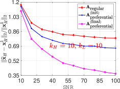
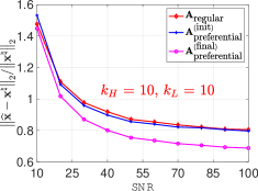
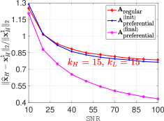
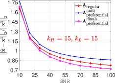
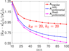
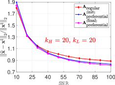
Figure 3: Comparison of preferential sensing vs regular sensing. The length $n_{H}$ of the high-priority part $\mathbf{x}^{\natural}_{H}$ is set as $100$; while the length $n_{L}$ of the low-priority part $\mathbf{x}^{\natural}_{L}$ is set as $400$. (Left panel) We evaluate the reconstruction performance w.r.t. the high-priority part $\|\widehat{\mathbf{x}}_{H}-\mathbf{x}^{\natural}_{H}\|_{2}/\|\mathbf{x}^{\natural}_{H}\|_{2}$. (Right panel) We evaluate the reconstruction performance w.r.t. the whole signal $\|\widehat{\mathbf{x}}-\mathbf{x}^{\natural}\|_{2}/\|\mathbf{x}^{\natural}\|_{2}$.

Impact of signal length

We also studied various settings in which the length $n_{H}$ of the high-priority part $\mathbf{x}^{\natural}_{H}$ is set to $\left\{150,200,250,300\right\}$ and the corresponding length $n_{L}$ of the low-priority part $\mathbf{x}^{\natural}_{L}$ is set to $\left\{600,800,1000,1200\right\}$. The simulation results are plotted in Fig. 4.

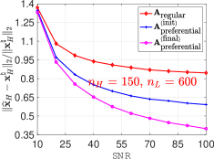
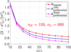
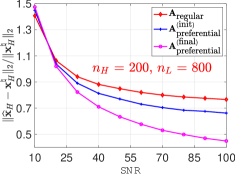
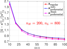
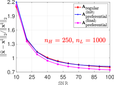
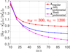
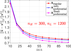
Figure 4: Comparison of preferential sensing vs regular sensing. Both the sparsity number $k_{H}$ and $k_{L}$ are set as $15$. (Left panel) We evaluate the reconstruction performance w.r.t. the high-priority part $\|\widehat{\mathbf{x}}_{H}-\mathbf{x}^{\natural}_{H}\|_{2}/\|\mathbf{x}^{\natural}_{H}\|_{2}$. (Right panel) We evaluate the reconstruction performance w.r.t. the whole signal $\|\widehat{\mathbf{x}}-\mathbf{x}^{\natural}\|_{2}/\|\mathbf{x}^{\natural}\|_{2}$.

Compared to regular sensing, our sensing matrix $\mathbf{A}^{(\textup{final})}_{\textup{preferential}}$ can reduce the error in the high-priority part $\mathbf{x}^{\natural}_{H}$ significantly. For example, when $\mathsf{SNR}=100$, the ratio $\|\widehat{\mathbf{x}}_{H}-\mathbf{x}^{\natural}_{H}\|_{2}/\|\mathbf{x}_{H}^{\natural}\|_{2}$ reduces between $40\%\sim 60\%$ with the sensing matrix $\mathbf{A}^{(\textup{final})}_{\textup{preferential}}$. Meanwhile, w.r.t. the whole signal $\mathbf{x}^{\natural}$, the ratio ${\left\|\widehat{\mathbf{x}}-\mathbf{x}^{\natural}\right\|}_{2}/{\left\|\mathbf{x}^{\natural}\right\|}_{2}$ decreases with a smaller magnitude.

Experiments with real-world data

We compare the performance of sensing matrices for images using $(i)$ MNIST dataset LeCun et al., (1998), which consists of $10000$ images in the testing set and $60000$ images in the training set; and $(ii)$ Lena image.

To obtain a sparse representation for each image, we perform a $2\textup{D}$ Haar transform ${\cal H}(\cdot)$, which generates four sub-matrices being called as the approximation coefficients (at the coarsest level), horizontal detail coefficients, vertical detail coefficients, and diagonal detail coefficients. The approximation coefficients are at the coarsest level and are treated as the high-priority part $\mathbf{x}^{\natural}_{H}$; while the horizontal detail coefficients, vertical detail coefficients, and diagonal detail coefficients are regarded as the low-priority part $\mathbf{x}^{\natural}_{L}$. Hence we can write the sensing relation in (1.1) as

$$\mathbf{y}=\mathbf{A}{\cal H}(\textup{Image})+\mathbf{w},$$ (6.1)

where Image denotes the input image, ${\cal H}(\cdot)$ denotes the vectorized version of the coefficients and is viewed as the sparse ground-truth signal, and $\mathbf{w}$ denotes the sensing noise. The sensing matrix $\mathbf{A}$ is designed such that the approximation coefficients of ${\cal H}(\textup{Image})$ can be better reconstructed.

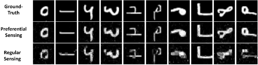
Figure 5: The performance comparison between the sensing matrix for preferential sensing $\mathbf{A}^{(\textup{final})}_{\textup{preferential}}$ and sensing matrix for regular sensing $\mathbf{A}_{\textup{regular}}$. (Top) The ground-truth images. (Middle) The reconstructed images with the sensing matrix $\mathbf{A}^{(\textup{final})}_{\textup{preferential}}$. (Bottom) The reconstructed images with the sensing matrix $\mathbf{A}_{\textup{regular}}$.

Experiments with MNIST

Experiment set-up. We set the images from MNIST as the input, which consists of $10000$ images in the testing set and $60000$ images in the training set with each image being of dimension $28\times 28$.

The whole datasets can be divided into $10$ categories with each category representing a digit from zero to nine. For each digit, we design one unique sensing matrix. The lengths $n_{H}$ and $n_{L}$ are set to $(28/2)^{2}=196$ and $3\times(28/2)^{2}=588$, respectively. The sparsity coefficients $k_{H}$ and $k_{L}$ varied among different digits.

Discussion. To evaluate the performance, we define ratios $r_{H,(\cdot)}$ and $r_{W,(\cdot)}$ as

$$r_{H,(\cdot)} \triangleq\frac{\|\widehat{\mathbf{x}}_{H}-\mathbf{x}^{\natural}_{H}\|_{2}}{\|\mathbf{x}^{\natural}_{H}\|_{2}};$$

$$r_{W,(\cdot)} \triangleq\frac{\|\widehat{\mathbf{x}}-\mathbf{x}^{\natural}\|_{2}}{\|\mathbf{x}^{\natural}\|_{2}},\vspace{1mm}$$

which correspond to the $\ell_{2}$ error in the high-priority part $\mathbf{x}^{\natural}_{H}$ and the entire signal $\mathbf{x}^{\natural}$, respectively. We use the sensing matrix $\mathbf{A}_{\textup{regular}}$ as the benchmark. In addition, we omit the results of $\mathbf{A}^{(\textup{init})}_{\textup{preferential}}$, since the sensing matrix $\mathbf{A}^{(\textup{final})}_{\textup{preferential}}$ has better performance.

The results are listed in Tab. 1. A subset of the reconstructed images are shown in Fig. 5. From Tab. 1 and Fig. 5, we conclude that our sensing matrix $\mathbf{A}^{(\textup{final})}_{\textup{preferential}}$ for the preferential sensing can better preserve the images when comparing with the sensing matrix $\mathbf{A}_{\textup{regular}}$ for the regular sensing.

	Training Set					Testing Set
Digit	$r_{H,(p)}$	$r_{H,(r)}$	$r_{W,(p)}$	$r_{W,(r)}$		$r_{H,(p)}$	$r_{H,(r)}$	$r_{W,(p)}$	$r_{W,(r)}$
$0$	0.28315	$0.5154$	0.44818	$0.60131$		0.30292	$0.45749$	0.46283	$0.56486$
$1$	0.16746	$0.33751$	0.29332	$0.41599$		0.1511	$0.45264$	0.2659	$0.51864$
$2$	0.26303	$0.50365$	0.42984	$0.59959$		0.24896	$0.4233$	0.42216	$0.52556$
$3$	0.24613	$0.43677$	0.42514	$0.53163$		0.26446	$0.46766$	0.43534	$0.56189$
$4$	0.28331	$0.44377$	0.44623	$0.53791$		0.30092	$0.4445$	0.45804	$0.53749$
$5$	0.28405	$0.53511$	0.45727	$0.6198$		0.27258	$0.47044$	0.44382	$0.56622$
$6$	0.28801	$0.39436$	0.45053	$0.51701$		0.27084	$0.5086$	0.44134	$0.59534$
$7$	0.25503	$0.41621$	0.41809	$0.52896$		0.27266	$0.51329$	0.41693	$0.5783$
$8$	0.31263	$0.51918$	0.47618	$0.61492$		0.32731	$0.48163$	0.48699	$0.5837$
$9$	0.30171	$0.54394$	0.45241	$0.61799$		0.27385	$0.55313$	0.43116	$0.62785$

Table 1: The index $i=p$ corresponds to the sensing matrix $\mathbf{A}^{(\textup{final})}_{\textup{preferential}}$ for the preferential sensing; while the index $i=r$ corresponds to the sensing matrix $\mathbf{A}_{\textup{regular}}$ for the regular sensing. We define the ratio $r_{H,(i)}$ ($i=\left\{p,r\right\}$) as the error w.r.t. the high priority part, namely, $\|\widehat{\mathbf{x}}_{H}-\mathbf{x}^{\natural}_{H}\|_{2}/\|\mathbf{x}^{\natural}_{H}\|_{2}$. Similarly we define the ratio $r_{W,(i)}$ ($i=\left\{p,r\right\}$) as the ratio w.r.t. the whole signal, namely, $\|\widehat{\mathbf{x}}-\mathbf{x}^{\natural}\|_{2}/\|\mathbf{x}^{\natural}\|_{2}$. Moreover, we put the results corresponding to the sensing matrix $\mathbf{A}^{(\textup{final})}_{\textup{preferential}}$ in the bold font.

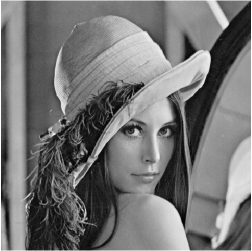
Figure 6: (Left) Ground-truth image. (Middle) Reconstructed image via sensing matrix $\mathbf{A}^{(\textup{final})}_{\textup{preferential}}$ for preferential sensing. (Right) Reconstructed image via sensing matrix $\mathbf{A}_{\textup{regular}}$ for regular sensing.

Experiments with Lena Image

Experiment set-up. We evaluate the benefits of using $\mathbf{A}^{(\textup{final})}_{\textup{preferential}}$ for the Lena image with dimension $512\times 512$. Notice that the sensing matrix would have been prohibitively large if we used the whole image as the input. To put more specifically, we would need a matrix with the width $512^{2}=262144$. To handle such issue, we divide the whole images into a set of sub-blocks with dimensions $32\times 32$ and design one sensing matrix with the width $32^{2}=1024$. For each sub-block, we first obtain a sparse representation with a 2D Haar transform and then reconstruct the signal in (6.1).

Discussion. The comparison of results is plotted in Fig. 6, from which we conclude that the sensing matrix $\mathbf{A}^{(\textup{final})}_{\textup{preferential}}$ has much better performance in image reconstruction in comparison with the sensing matrix $\mathbf{A}_{\textup{regular}}$. The ratios $r_{H,(p)}$ and $r_{H,(r)}$ are computed as $0.0446$ and $0.3029$, respectively; while the ratio $r_{W,(p)}$ and $r_{W,(r)}$ are computed as $0.0709$ and $0.3144$, respectively.

The degree distributions $\lambda_{H}(\cdot)$ and $\lambda_{L}(\cdot)$ of the variable nodes for the sensing matrix $\mathbf{A}^{(\textup{final})}_{\textup{preferential}}$ are obtained as

$$\lambda_{H}(\alpha)$$

$$=0.0057856\alpha+0.025915\alpha^{2}+0.36394\alpha^{3}+0.35183\alpha^{4}$$

$$+0.10333\alpha^{5}+0.04134\alpha^{6}+0.021619\alpha^{7}+0.013508\alpha^{8}$$

$$+0.0094374\alpha^{9}+0.0070906\alpha^{10}+0.0056\alpha^{11}$$

$$+0.0045851\alpha^{12}+0.0038574\alpha^{13}+0.0033145\alpha^{14}$$

$$+0.0028963\alpha^{15}+.0025659\alpha^{16}+0.0022992\alpha^{17}$$

$$+0.0020801\alpha^{18}+0.0018973\alpha^{19}+0.0017428\alpha^{20}$$

$$+0.0016109\alpha^{21}+0.001497\alpha^{22}+0.001398\alpha^{23}$$

$$+0.0013111\alpha^{24}+0.0012344\alpha^{25}+0.0011662\alpha^{26}$$

$$+0.0011053\alpha^{27}+0.0010506\alpha^{28}+0.0010013\alpha^{29}$$

$$+0.0009565\alpha^{30}+0.00091576\alpha^{31}+0.00087852\alpha^{32}$$

$$+0.00084436\alpha^{33}+0.00081292\alpha^{34}+0.00078388\alpha^{35}$$

$$+0.00075697\alpha^{36}+0.00073197\alpha^{37}+0.00070867\alpha^{38}$$

$$+0.00068691\alpha^{39}+0.00066652\alpha^{40}+0.00064738\alpha^{41}$$

$$+0.00062937\alpha^{42}+0.00061238\alpha^{43}+0.00059633\alpha^{44}$$

$$+0.00058114\alpha^{45}+0.00056673\alpha^{46}+0.00055304\alpha^{47}$$

$$+0.00054001\alpha^{48}+0.0005276\alpha^{49};$$

$$\lambda_{L}(\alpha)=\alpha.\vspace{1mm}$$

The check node degrees $\mathsf{dc}_{\mathsf{H}}$ and $\mathsf{dc}_{\mathsf{L}}$ are both set as $4$. Meanwhile, the sensing matrix $\mathbf{A}_{\textup{regular}}$ designed in (3.7) is a regular sensing matrix whose variable node and check node degree distributions are given by $\lambda(\alpha)=\alpha^{2}$ and $\rho(\alpha)=\alpha^{7}$, respectively.

Conclusions

This paper presented a general framework of the sensing matrix design for a linear measurement system. Focusing on a sparse sensing matrix $\mathbf{A}$, we associated it with a graphical model ${\cal G}=({\cal V},{\cal E})$ and transformed the design of $\mathbf{A}$ to the connectivity problem in ${\cal G}$. With the density evolution technique, we proposed two design strategies, i.e., regular sensing and preferential sensing. In the regular sensing scenario, all entries of the signal are recovered with equal accuracy; while in the preferential sensing scenario, the entries in the high-priority sub-block are recovered more accurately (or exactly) relative to the entries in the low-priority sub-block. We then analyzed the impact of the connectivity of the graph on the recovery performance. For the regular sensing, our framework can reproduce the classical result of Lasso, i.e., the number of measurements $m$ should be at least in the order $O(k\log n)$, where $n$ is the length of the signal and $k$ is the sparsity number. For the preferential sensing, our framework can lead to a significant reduction of the reconstruction error in the high-priority part and a modest reduction of the error in the whole signal. Numerical experiments with both synthetic data and real-world data are presented to corroborate our claims.

Appendix A Proof of Thm. 3.3

Proof.

We begin the proof by restating the DE equation w.r.t. $E^{(t+1)}$ and $V^{(t+1)}$ as

$$E^{(t+1)}=\underbrace{\mathbb{E}_{\textup{prior}(s),z\sim\mathsf{N}(0,1)}\left[\mathsf{prox}\left(s+a_{1}z\sqrt{E^{(t)}};\beta a_{2}V^{(t)}\right)-s\right]^{2}}_{\triangleq\Psi_{E}\left(E^{(t)};V^{(t)}\right)};$$

$$V^{(t+1)}=\underbrace{\mathbb{E}_{\textup{prior}(s),z\sim\mathsf{N}(0,1)}\left[\beta a_{2}V^{(t)}\mathsf{prox}^{{}^{\prime}}\left(s+a_{1}z\sqrt{E^{(t)}};\beta a_{2}V^{(t)}\right)\right]}_{\triangleq\Psi_{V}\left(E^{(t)};V^{(t)}\right)}.\vspace{1mm}$$

The derivation of the necessary conditions for $\lim_{t\rightarrow\infty}\left(E^{(t)},V^{(t)}\right)=\left(0,0\right)$ consists of two parts:

• Part I. We verify that $(0,0)$ is a fixed-point of the DE equation;

• Part II. We consider the necessary condition such that DE equation converges within the proximity of the origin points, i.e., $E^{(t)}$ and $V^{(t)}$ are close to zero.

Since Part I can be easily verified, we put our major focus on Part II. Define the difference across iterations as $\delta^{(t)}_{E}=E^{(t+1)}-E^{(t)}$ and $\delta^{(t)}_{V}=V^{(t+1)}-V^{(t)}$, we would like to show $\lim_{t\rightarrow\infty}(\delta_{E}^{(t)},\delta_{V}^{(t)})=\left(0,0\right)$. With Taylor expansion, we obtain

$$\delta^{(t+1)}_{E}=~{} \Psi_{E}\left(E^{(t+1)},V^{(t+1)}\right)-\Psi_{E}\left(E^{(t)},V^{(t)}\right)$$

$$=~{} \left(\frac{\partial\Psi_{E}\left(E,V\right)}{\partial E}\left|{}_{E=E^{(t)},V=V^{(t)}}\right.\right)\cdot\delta_{E}^{(t)}$$

$$+~{} \left(\frac{\partial\Psi_{E}\left(E,V\right)}{\partial V}\left|{}_{E=E^{(t)},V=V^{(t)}}\right.\right)\cdot\delta_{V}^{(t)}$$

$$+~{} O\left(\left(\delta_{E}^{(t)}\right)^{2}\right)+O\left(\left(\delta_{V}^{(t)}\right)^{2}\right).$$ (A.1)

Consider the region where $\delta_{E}^{(t)}$ and $\delta_{V}^{(t)}$ are sufficiently small, we require $\delta_{E}^{(t)}$ and $\delta_{V}^{(t)}$ to converge to zero. Notice the quadratic terms in (A) can be safely omitted in this region. Denote the gradients $\left(\frac{\partial\Psi_{E}\left(E,V\right)}{\partial E}\right)^{(t)}\left|{}_{E=E^{(t)},V=V^{(t)}}\right.$, $\frac{\partial\Psi_{E}\left(E,V\right)}{\partial V}\left|{}_{E=E^{(t)},V=V^{(t)}}\right.$, $\frac{\partial\Psi_{V}\left(E,V\right)}{\partial E}\left|{}_{E=E^{(t)},V=V^{(t)}}\right.$, and $\frac{\partial\Psi_{V}\left(E,V\right)}{\partial V}\left|{}_{E=E^{(t)},V=V^{(t)}}\right.$ as $\left(\frac{\partial\Psi_{E}\left(E,V\right)}{\partial E}\right)^{(t)}$, $\left(\frac{\partial\Psi_{E}\left(E,V\right)}{\partial V}\right)^{(t)}$, $\left(\frac{\partial\Psi_{V}\left(E,V\right)}{\partial E}\right)^{(t)}$, and $\left(\frac{\partial\Psi_{V}\left(E,V\right)}{\partial V}\right)^{(t)}$, respectively. We obtain the linear equation

$$\begin{bmatrix}\delta_{E}^{(t+1)}\\ \delta_{V}^{(t+1)}\end{bmatrix}=~{} \ \underbrace{\begin{bmatrix}\left(\frac{\partial\Psi_{E}\left(E,V\right)}{\partial E}\right)^{(t)}&\left(\frac{\partial\Psi_{E}\left(E,V\right)}{\partial V}\right)^{(t)}\\ \left(\frac{\partial\Psi_{V}\left(E,V\right)}{\partial E}\right)^{(t)}&\left(\frac{\partial\Psi_{V}\left(E,V\right)}{\partial V}\right)^{(t)}\end{bmatrix}}_{\triangleq\mathbf{L}^{(t)}}\begin{bmatrix}\delta_{E}^{(t)}\\ \delta_{V}^{(t)}\end{bmatrix},\vspace{1mm}$$

and would require the lower bound of the operator norm of the matrix $\mathbf{L}^{(t)}$ to be no greater than $1$, i.e., $\inf_{t}{\left\|\mathbf{L}^{(t)}\right\|}_{\textup{OP}}\leq 1$, since otherwise the values of $\delta_{E}^{(t)}$ and $\delta_{V}^{(t)}$ will keep increasing. Exploiting the fact $\frac{\partial\Psi_{V}\left(E,V\right)}{\partial E}=0$, we conclude

$${\left\|\mathbf{L}^{(t)}\right\|}_{\textup{OP}}=\max\left[\left(\frac{\partial\Psi_{E}\left(E,V\right)}{\partial E}\right)^{(t)},\left(\frac{\partial\Psi_{V}\left(E,V\right)}{\partial V}\right)^{(t)}\right].\vspace{1mm}$$

The proof is then concluded by computing the lower bounds of the gradients $\frac{\partial\Psi_{E}\left(E,V\right)}{\partial E}$ and $\frac{\partial\Psi_{V}\left(E,V\right)}{\partial V}$ as

$$\frac{\partial\Psi_{E}\left(E,V\right)}{\partial E}\left|{}_{E=E^{(t)},V=V^{(t)}}\right.$$

$$=~{} a_{1}^{2}\cdot\mathbb{E}_{\textup{prior}(s)}\left[\Phi\left(-\frac{s+a_{2}V^{(t)}}{a_{1}\sqrt{E^{(t)}}}\right)+\Phi\left(\frac{s-a_{2}V^{(t)}}{a_{1}\sqrt{E^{(t)}}}\right)\right]$$

$$\stackrel{{\scriptstyle\small{\raisebox{0.6pt}{\raisebox{-.8pt}{1}⃝}}}}{{=}}~{} \frac{a_{1}^{2}k}{n}\left[\Phi\left(-\frac{c_{0}+a_{2}V^{(t)}}{a_{2}\sqrt{E^{(t)}}}\right)+\Phi\left(\frac{c_{0}-a_{2}V^{(t)}}{a_{1}\sqrt{E^{(t)}}}\right)\right]$$

$$+~{} 2a_{1}^{2}\left(1-\frac{k}{n}\right)\Phi\left(-\frac{a_{2}V^{(t)}}{a_{1}E^{(t)}}\right)$$

$$\stackrel{{\scriptstyle\small{\raisebox{0.6pt}{\raisebox{-.8pt}{2}⃝}}}}{{\rightarrow}}~{} \frac{ka_{1}^{2}}{n}+2a_{1}^{2}\left(1-\frac{k}{n}\right)\Phi\left(-\frac{a_{2}V^{(t)}}{\sqrt{a_{1}E^{(t)}}}\right)\stackrel{{\scriptstyle\small{\raisebox{0.6pt}{\raisebox{-.8pt}{3}⃝}}}}{{\geq}}\frac{ka_{1}^{2}}{n};$$

$$\frac{\partial\Psi_{V}\left(E,V\right)}{\partial V}\left|{}_{E=E^{(t)},V=V^{(t)}}\right.$$

$$=~{} \beta a_{2}\cdot\mathbb{E}_{\textup{prior}(s)}\left[\Phi\left(-\frac{s+a_{2}V^{(t)}}{a_{1}\sqrt{E^{(t)}}}\right)+\Phi\left(\frac{s-a_{2}V^{(t)}}{a_{1}\sqrt{E^{(t)}}}\right)\right]$$

$$\stackrel{{\scriptstyle\small{\raisebox{0.6pt}{\raisebox{-.8pt}{4}⃝}}}}{{=}}~{} \frac{\beta a_{2}k}{n}\left[\Phi\left(-\frac{c_{0}+a_{2}V^{(t)}}{a_{1}\sqrt{E^{(t)}}}\right)+\Phi\left(\frac{c_{0}-a_{2}V^{(t)}}{a_{1}\sqrt{E^{(t)}}}\right)\right]$$

$$+~{} 2\beta a_{2}\left(1-\frac{k}{n}\right)\Phi\left(-\frac{a_{2}V^{(t)}}{a_{1}E^{(t)}}\right)$$

$$\stackrel{{\scriptstyle\small{\raisebox{0.6pt}{\raisebox{-.8pt}{5}⃝}}}}{{\rightarrow}}~{} \frac{k\beta a_{2}}{n}+2\beta a_{2}\left(1-\frac{k}{n}\right)\Phi\left(-\frac{a_{2}V^{(t)}}{\sqrt{a_{1}E^{(t)}}}\right)\stackrel{{\scriptstyle\small{\raisebox{0.6pt}{\raisebox{-.8pt}{6}⃝}}}}{{\geq}}\frac{k\beta a_{2}}{n},$$ (A.2)

where $\Phi(\cdot)=(2\pi)^{-1/2}\int_{-\infty}^{(\cdot)}e^{-z^{2}/2}dz$ is the CDF of the standard normal RV $z$, namely, $z\sim\mathsf{N}(0,1)$. In \raisebox{-.8pt}{1}⃝ and \raisebox{-.8pt}{4}⃝ we use the prior distribution $\textup{prior}(s)=k/n\cdot\mathbbm{1}(c_{0})+(1-k/n)\mathbbm{1}(0)$. Further, in \raisebox{-.8pt}{2}⃝ and \raisebox{-.8pt}{5}⃝ we use the fact

$$\lim_{E^{(t)}\rightarrow 0}\Phi\left(-\frac{c_{0}+a_{2}V^{(t)}}{\sqrt{a_{1}E^{(t)}}}\right)+\Phi\left(\frac{c_{0}-a_{2}V^{(t)}}{\sqrt{a_{1}E^{(t)}}}\right)=1,\vspace{1mm}$$

since $c_{0}\neq 0$. Finally, in \raisebox{-.8pt}{3}⃝ and \raisebox{-.8pt}{6}⃝ we omit the non-negative terms $\Phi(\cdot)$.

∎

Appendix B Example of regular sensing with a Gaussian prior

In addition to the Laplacian prior studied in Subsec. 3.3, we also investigate the Gaussian prior. Assuming the ground-truth $\mathbf{x}^{\natural}$ to be Gaussian distributed with zero mean and unit variance, we would like to recover the signal $\mathbf{x}^{\natural}$ with the regularizer $f(\mathbf{x})={\left\|\mathbf{x}\right\|}_{2}^{2}$. In this case, the DE equation reduces to

$$E^{(t+1)} =\frac{a_{1}^{2}E^{(t)}+a_{2}^{2}(V^{(t)})^{2}}{\left(1+a_{2}V^{(t)}\right)^{2}};$$

$$V^{(t+1)} =\frac{a_{2}V^{(t)}}{1+a_{2}V^{(t)}},$$ (B.1)

where $a_{1},a_{2}$ are defined the same as above. Then we have the following theorem.

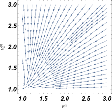
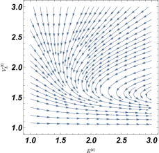
Figure 7: Illustration of DE in (B) when setting $\textup{prior}(s)=\mathbbm{1}(s=1)$. Left panel: $\sum_{i,j}\rho_{i}\lambda_{j}\sqrt{i/j}<1$. Right panel: $\sum_{i,j}\rho_{i}\lambda_{j}\sqrt{i/j}>1$. Notice that the left panel has a fix-point $(0,0)$ while the right panel is with non-zero fix-point.

Provided that $\sum_{i,j}\rho_{i}\lambda_{j}\sqrt{i/j}<1$, the average error $E^{(t)}$ and the variance $V^{(t)}$ decrease exponentially after some iteration index $T$, that is, $E^{(t)}\leq e^{-c_{0}(t-T)}E^{(T)}$ and $V^{(t)}\leq e^{-c_{1}(t-T)}V^{(T)}$ whenever $t\geq T$, where $c_{0},c_{1}>0$ are some fixed constants.

An illustration of the DE in (B) is shown in Fig. 7.

Proof.

We begin the proof by restating that the functions $\mathbb{E}_{z}h_{\textup{mean}}(\cdot;\cdot)$ and $\mathbb{E}_{z}h_{\textup{var}}\left(\textup{mean};\textup{var}\right)$ are written as

$$\mathbb{E}_{z}h_{\textup{mean}}\left(s+a_{1}z\sqrt{E^{(t)}};a_{2}V^{(t)}\right) =\ \frac{a_{1}^{2}E^{(t)}+a_{2}^{2}\left(V^{(t)}\right)^{2}s^{2}}{\left(1+a_{2}V^{(t)}\right)^{2}};$$

$$\mathbb{E}_{z}h_{\textup{var}}\left(s+a_{1}z\sqrt{E^{(t)}};a_{2}V^{(t)}\right) =\ \frac{a_{2}V^{(t)}}{1+a_{2}V^{(t)}},\vspace{1mm}$$

which can be easily verified. Then we prove that $V^{(t)}$ decreases exponentially since $a_{2}>0$ and hence for an arbitrary time index $T_{1}$ the relation

$$V^{(t)}\leq\left(\frac{a_{2}}{1+a_{2}}\right)^{t-T_{1}}V^{(T_{1})}=e^{-c_{1}\left(t-T_{1}\right)}V^{(T_{1})}\vspace{1mm}$$

holds for $t\geq T_{1}$, where $c_{1}$ is defined as $\log(1+a_{2}^{-1})>0$.

Afterwards, we study the behavior of $E^{(t)}$. Denote $V_{S}$ as $\mathbb{E}_{\textup{prior}(s)}(s^{2})$, we have

$$E^{(t+1)}\leq~{} a_{1}^{2}E^{(t)}+\frac{a_{2}V_{S}V^{(t)}}{2}$$

$$\stackrel{{\scriptstyle\small{\raisebox{0.6pt}{\raisebox{-.8pt}{1}⃝}}}}{{\leq}}~{} a_{1}^{2}E^{(t)}+\frac{a_{2}V_{S}}{2}\left(\frac{a_{2}}{1+a_{2}}\right)^{t}V^{(0)},$$ (B.2)

where in \raisebox{-.8pt}{1}⃝ we use the relation $V^{(t)}\leq\left(a_{2}/(1+a_{2})\right)^{t}V^{(0)}$. Define a new sequence $\widetilde{E}^{(t)}=E^{(t)}/a_{1}^{2t}$, we can transform (B) to

$$\widetilde{E}^{(t+1)}=~{} \frac{E^{(t+1)}}{a_{1}^{2(t+1)}}\leq\frac{E^{(t)}}{a_{1}^{2t}}+\frac{a_{2}V_{S}V^{(0)}}{2a_{1}^{2}}\left(\frac{a_{2}}{(1+a_{2})a_{1}^{2}}\right)^{t}$$

$$=~{} \widetilde{E}^{(t)}+\frac{a_{2}V_{S}V^{(0)}}{2a_{1}^{2}}\left(\frac{a_{2}}{(1+a_{2})a_{1}^{2}}\right)^{t},\vspace{1mm}$$

after rearranging the terms. Due to the time-invariance, we also have the relation

$$\widetilde{E}^{(t)}\leq\widetilde{E}^{(t-1)}+\frac{a_{2}V_{S}V^{(0)}}{2a_{1}^{2}}\left(\frac{a_{2}}{(1+a_{2})a_{1}^{2}}\right)^{t-1}.\vspace{1mm}$$

Iterating over all such inequalities, we obtain the equation

$$\widetilde{E}^{(t+1)}\leq\widetilde{E}^{(1)}+\frac{a_{2}V_{S}V^{(0)}}{2a_{1}^{2}}\frac{\frac{a_{2}}{(1+a_{2})a_{1}^{2}}\left(1-\left(\frac{a_{2}}{(1+a_{2})a_{1}^{2}}\right)^{t}\right)}{1-\left(\frac{a_{2}}{(1+a_{2})a_{1}^{2}}\right)},$$

which leads to

$$E^{(t+1)}\leq a_{1}^{2t}E^{(1)}+\underbrace{\frac{a_{2}V_{S}V^{(0)}}{2a_{1}^{2}}\cdot\frac{a_{2}}{1+a_{2}}\frac{a_{1}^{2t}-\left(\frac{a_{2}}{1+a_{2}}\right)^{t}}{1-\frac{a_{2}}{(1+a_{2})a_{1}^{2}}}}_{I}.$$ (B.3)

Since $a_{1}<1$ and $a_{2}/(1+a_{2})<1$, we have the second term $I$ in (B.3) to be negligible as $t$ goes to infinity. Hence we can choose a sufficiently large $T$ such that for $t\geq T$, we have $E^{(t+1)}$ is approximately equal to $a_{1}^{2t}E^{(1)}$ and conclude the exponential decay of $E^{(t)}$. ∎

Discussion of the DE for both regular and irregular designs

First we explain the physical meaning of the quantities $E^{(t)}$ and $V^{(t)}$, which track the average error and the average variance at the $t$th iteration, respectively. Since the physical meaning of $V^{(t)}$ can be easily obtained, we focus on the explanation of $E^{(t)}$. For the convenience of the analysis, we rewrite the MAP estimator as

$$\widehat{\mathbf{x}}=\textup{argmax}_{\mathbf{x}}\exp\left(-\frac{\gamma{\left\|\mathbf{y}-\mathbf{A}\mathbf{x}\right\|}_{2}^{2}}{2\sigma^{2}}\right)\cdot\exp\left(-\gamma f(\mathbf{x})\right),\vspace{1mm}$$

where $\gamma>0$ is a redundant positive constant. Then we restate the message-passing algorithm, which is used to solve the MAP estimator, as

$$\widehat{m}_{a\rightarrow i}^{(t+1)}(x_{i}) \cong\int\prod_{j\in\partial a\setminus i}m_{j\rightarrow a}^{(t)}(x_{i})\times e^{-\frac{\gamma\left(y_{a}-\sum_{j=1}^{n}A_{aj}x_{j}\right)^{2}}{2\sigma^{2}}}dx_{j}$$

$$m_{i\rightarrow a}^{(t+1)}(x_{i}) \cong e^{-\gamma f(x_{i})}\prod_{b\in\partial i\setminus a}\widehat{m}_{b\rightarrow i}^{(t+1)}(x_{i}).\vspace{1mm}$$

The MAP estimator of $\widehat{x}_{i}$ is hence written as

$$\widehat{x}_{i}=\textup{argmax}_{x_{i}}\mathbb{P}\left(x_{i}|\mathbf{y}\right)\approx\textup{argmax}_{x_{i}}e^{-\gamma f(x_{i})}\prod_{a\in\partial i}\widehat{m}_{a\rightarrow i}^{(t)}(x_{i}).\vspace{1mm}$$

Notice that $\widehat{x}_{i}$ can be rewritten as the mean w.r.t. the probability measure $e^{-\gamma f(x_{i})}\prod_{a\in\partial i}\widehat{m}_{a\rightarrow i}^{(t)}$, namely,

$$\widehat{x}_{i}\approx\int_{x_{i}}x_{i}e^{-\gamma f(x_{i})}\ \prod_{a\in\partial i}\widehat{m}_{a\rightarrow i}^{(t)}(x_{i})dx_{i},\vspace{1mm}$$

by letting $\gamma\rightarrow\infty$. Since the mean $\mu_{i\rightarrow a}$ is computed as

$$\mu_{i\rightarrow a}=\int_{x_{i}}x_{i}e^{-\gamma f(x_{i})}\ \prod_{b\in\partial i\setminus a}\widehat{m}_{b\rightarrow i}^{(t)}(x_{i})dx_{i},\vspace{1mm}$$

which is close to $\widehat{x}_{i}$, we obtain the approximation $m^{-1}\sum_{a=1}^{m}(\mu_{i\rightarrow a}-x_{i}^{\natural})^{2}$ as $(\widehat{x}_{i}-x_{i}^{\natural})^{2}$. We then conclude

$$E^{(t)}=\frac{1}{mn}\sum_{i=1}^{n}\sum_{a=1}^{m}\left(\mu_{i\rightarrow a}-x_{i}^{\natural}\right)^{2}\approx\frac{1}{n}\sum_{i=1}^{n}\left(\widehat{x}_{i}-x_{i}^{\natural}\right)^{2},\vspace{1mm}$$

which is approximately the average of error at the $t$th iteration. Having discussed the physical meaning of the quantities $E^{(t)}$ and $V^{(t)}$, we turn to the derivation of the DE equation.

Supporting Lemmas

We begin the derivation with the following lemma, which is stated as Consider the message flow $\widehat{m}_{a\rightarrow i}^{(t+1)}$ from the check node $a$ to the variable node $i$ and approximate it as a Gaussian RV with mean $\widehat{\mu}_{a\rightarrow i}^{(t+1)}$ and variance $\widehat{v}_{a\rightarrow i}^{(t+1)}$, i.e., $\widehat{m}_{a\rightarrow i}^{(t+1)}\sim\mathsf{N}\left(\widehat{\mu}_{a\rightarrow i}^{(t+1)},\widehat{v}_{a\rightarrow i}^{(t+1)}\right)$. Then, we can obtain the following update equation at the $(t+1)$th iteration

$$\widehat{\mu}_{a\rightarrow i}^{(t+1)} =x_{i}+A\sum_{j\in\partial a\setminus i}A_{ai}A_{aj}\left(x_{j}-\ \mu_{j\rightarrow a}^{(t)}\right)+AA_{ai}w_{a};$$

$$\widehat{v}_{a\rightarrow i}^{(t+1)} =A\sigma^{2}+|\partial a|V^{(t)},\vspace{1mm}$$

where $|\partial a|$ denotes the degree of the check node $a$.

Proof.

Consider the message flow $\widehat{m}_{a\rightarrow i}^{(t+1)}$ from check-node to variable node at the $(t+1)$th iteration

$$\widehat{m}_{a\rightarrow i}^{(t+1)}=~{} \frac{1}{Z_{a\rightarrow i}^{t}}\int\prod_{j\in\partial a\setminus i}m_{j\rightarrow a}^{(t)}(x_{j})$$

$$\times~{} \exp\left(-\frac{\gamma\left(y_{a}-\sum_{j=1}A_{aj}x_{j}\right)^{2}}{2\sigma^{2}}\right)dx_{j}.$$ (3.1)

Approximate the message flow $m_{j\rightarrow a}^{(t+1)}$ as a Gaussian RV with mean $\mu_{j\rightarrow a}^{(t+1)}$ and variance $v_{j\rightarrow a}^{(t+1)}$. Plugging into (3.1) yields

$$\widehat{m}_{a\rightarrow i}^{(t+1)}=~{} \frac{1}{Z_{a\rightarrow i}^{t}}\int\prod_{j\in\partial a\setminus i}\exp\left[-\frac{\gamma\left(x_{j}-\mu_{j\rightarrow a}^{(t)}\right)^{2}}{2v_{j\rightarrow a}^{(t+1)}}\right]$$

$$\times~{} \exp\left(-\frac{\gamma\left(y_{a}-\sum_{j=1}A_{aj}x_{j}\right)^{2}}{2\sigma^{2}}\right)dx_{j}.$$ (3.2)

The direct calculation of the above integral involves the cross terms such as $A_{aj_{1}}A_{aj_{2}}x_{j_{1}}x_{j_{2}}$ ($j_{1}\neq j_{2}$), which can be cumbersome. To handle this issue, we adopt the trick in Nishimori, (2001); Krzakala et al., (2012a), whose basic idea is to introduce a redundant variable $\omega$ and exploit the relation

$$e^{-\frac{t^{2}}{2\sigma^{2}}}=\frac{1}{\sqrt{2\pi\sigma^{2}}}\int e^{-\frac{\omega^{2}}{2\sigma^{2}}+\frac{it\omega}{\sigma^{2}}}d\omega,\vspace{1mm}$$

where $t$ is an arbitrary number. As such, we can transform (3.1) to

$$\widehat{m}_{a\rightarrow i}^{(t+1)} \cong\int d\omega\prod_{j\in\partial a\setminus i}dx_{j}\cdot\exp\left[-\frac{\gamma\left(x_{j}-\mu_{j\rightarrow a}^{(t)}\right)^{2}}{2v_{j\rightarrow a}^{(t+1)}}\right]$$

$$\times\exp\left[-\frac{i\omega\gamma\left(y_{a}-\sum_{j=1}A_{aj}x_{j}\right)}{\sigma^{2}}\right]\cdot\exp\left[-\frac{\gamma\omega^{2}}{2\sigma^{2}}\right],$$

which diminishes the cross term $x_{j_{1}}x_{j_{2}}$ ($j_{1}\neq j_{2}$). Rearranging the terms for each $x_{j}$, we can iteratively perform the integral such that

$$\int dx_{j}\cdot\exp\left(-\frac{\gamma\left(x_{j}-\mu_{j\rightarrow a}^{(t)}\right)^{2}}{2v_{j\rightarrow a}^{(t)}}+\frac{i\omega\gamma A_{aj}x_{j}}{\sigma^{2}}\right)$$

$$=~{} \sqrt{\frac{2\pi v_{j\rightarrow a}^{(t)}}{\gamma}}\cdot\exp\left[-\frac{\gamma(\widehat{\mu}_{j\rightarrow a}^{(t)})^{2}}{2\widehat{v}_{j\rightarrow a}^{(t)}}+\frac{v_{j\rightarrow a}^{(t)}\left(\frac{\gamma\mu_{j\rightarrow a}^{(t)}}{v_{j\rightarrow a}^{(t)}}+\frac{i\gamma\omega A_{aj}}{\sigma^{2}}\right)^{2}}{2\gamma}\right]$$

$$=~{} \sqrt{\frac{2\pi v_{j\rightarrow a}^{(t)}}{\gamma}}\cdot\exp\left(-\frac{\gamma\omega^{2}A_{aj}^{2}v_{j\rightarrow a}^{(t)}}{2\sigma^{4}}+\frac{i\gamma\omega A_{aj}\mu_{j\rightarrow a}^{(t)}}{\sigma^{2}}\right).$$

With some algebraic manipulations, we can compute its mean $\widehat{\mu}_{a\rightarrow i}^{(t+1)}$ and its variance $\widehat{v}_{a\rightarrow i}^{(t+1)}$ as

$$\widehat{\mu}_{a\rightarrow i}^{(t+1)} =\frac{A_{ai}\left(y_{a}-\sum_{j\in\partial a\setminus i}A_{aj}\mu_{j\rightarrow a}^{(t)}\right)}{A_{ai}^{2}};$$

$$\widehat{v}_{a\rightarrow i}^{(t+1)} =\ \frac{\sigma^{2}+\sum_{j\in\partial a\setminus i}A_{aj}^{2}v_{j\rightarrow a}^{(t)}}{A_{ai}^{2}}.$$

The following analysis focuses on how to approximate these two values. We begin by the discussion w.r.t. the variance $\widehat{v}_{a\rightarrow i}^{(t+1)}$. Note we have

$$\widehat{v}_{a\rightarrow i}^{(t+1)}\stackrel{{\scriptstyle\small{\raisebox{0.6pt}{\raisebox{-.8pt}{1}⃝}}}}{{\approx}}A\sigma^{2}+\sum_{j\in\partial a\setminus i}v_{j\rightarrow a}^{(t)},\vspace{1mm}$$

where in \raisebox{-.8pt}{1}⃝ we use $A_{ai}^{2}\approx\mathbb{E}\left(A_{ai}^{2}|A_{ai}\neq 0\right)=A^{-1}$ for $i\in\partial a$. As for the sum $\sum_{j\in\partial a\setminus i}v_{j\rightarrow a}^{(t)}$, we can view it to be randomly sampled from the set of variances $\left\{v_{j\rightarrow a}^{(t)}\right\}$ and approximate it as

$$\sum_{j\in\partial a\setminus i}v_{j\rightarrow a}^{(t)}\approx\left(|\partial a|-1\right)V^{(t)}\approx|\partial a|V^{(t)}.\vspace{1mm}$$

Notice that the variance is closely related with the check node degree $|\partial a|$. Having obtained the variance $\widehat{v}_{a\rightarrow i}^{(t+1)}$, we turn to the mean $\widehat{\mu}_{a\rightarrow i}^{(t+1)}$, which is computed as

$$\widehat{\mu}_{a\rightarrow i}^{(t+1)}=~{} \frac{A_{ai}\left(y_{a}-\sum_{j\in\partial a\setminus i}A_{aj}\mu_{j\rightarrow a}^{(t)}\right)}{A_{ai}^{2}}$$

$$\stackrel{{\scriptstyle\small{\raisebox{0.6pt}{\raisebox{-.8pt}{2}⃝}}}}{{\approx}}~{} AA_{ai}\left(A_{ai}x_{i}+\sum_{j\in\partial a\setminus i}A_{aj}\left(x_{j}-\ \mu_{j\rightarrow a}^{(t)}\right)+w_{a}\right)$$

$$\stackrel{{\scriptstyle\small{\raisebox{0.6pt}{\raisebox{-.8pt}{3}⃝}}}}{{\approx}}~{} x_{i}+A\sum_{j\in\partial a\setminus i}A_{ai}A_{aj}\left(x_{j}-\ \mu_{j\rightarrow a}^{(t)}\right)+AA_{ai}w_{a},$$

where in \raisebox{-.8pt}{2}⃝ and \raisebox{-.8pt}{3}⃝ we use the approximation $A^{2}_{ai}\approx A^{-1}$ for $i\in\partial a$.

∎

Derivation of DE

We study the message flow $m_{i\rightarrow a}^{(t+1)}$ from the variable node $i$ to the check node $a$

$$m_{i\rightarrow a}^{(t+1)}\cong e^{-\gamma f(x_{i})}\prod_{b\in\partial i\setminus a}e^{-\frac{\gamma\left(x_{i}-\widehat{\mu}_{b\rightarrow i}^{(t+1)}\right)^{2}}{2\widehat{v}_{b\rightarrow i}^{(t+1)}}}.\vspace{1mm}$$

To begin with, we study the product $\prod_{b\in\partial i\setminus a}\exp\bigg{(}-\frac{\gamma\left(x_{i}-\widehat{\mu}_{b\rightarrow i}^{(t+1)}\right)^{2}}{2\widehat{v}_{b\rightarrow i}^{(t)}}\bigg{)}$. Its variance $\widetilde{v}_{i\rightarrow a}^{(t+1)}$ is approximately computed as

$$\frac{\gamma}{\widetilde{v}_{i\rightarrow a}^{(t+1)}}\approx\ \sum_{b\in\partial i\setminus a}\frac{\gamma}{\widehat{v}_{b\rightarrow i}^{(t+1)}},\vspace{1mm}$$

which yields

$$\widetilde{v}_{i\rightarrow a}^{(t+1)}=\ \left(\frac{|\partial i|-1}{A\sigma^{2}+|\partial a|V^{(t)}}\right)^{-1}\approx\frac{A\sigma^{2}+|\partial a|V^{(t)}}{|\partial i|}.\vspace{1mm}$$

Further, the mean $\widetilde{\mu}_{i\rightarrow a}^{(t+1)}$ is calculated as

$$\widetilde{\mu}_{i\rightarrow a}^{(t+1)}=\left(\sum_{b\in\partial i\setminus a}\frac{\widehat{\mu}_{b\rightarrow i}^{(t+1)}}{\widehat{v}_{b\rightarrow i}^{(t+1)}}\right)/\ \left(\sum_{b\in\partial i\setminus a}\frac{1}{\widehat{v}_{b\rightarrow i}^{(t+1)}}\right)^{-1}$$

$$\stackrel{{\scriptstyle\small{\raisebox{0.6pt}{\raisebox{-.8pt}{1}⃝}}}}{{=}}~{} \ \frac{A\sigma^{2}+|\partial a|V^{(t)}}{|\partial i|}$$

$$\times~{} \left(\sum_{b\in\partial i\setminus a}\frac{x_{i}+A\sum_{j\in\partial b\setminus i}A_{bi}A_{bj}\left(x_{j}-\ \mu_{j\rightarrow b}^{(t)}\right)+AA_{bi}w_{b}}{A\sigma^{2}+|\partial a|V^{(t)}}\right)$$

$$\approx~{} \ x_{i}+\frac{A}{|\partial i|}\ \left[\sum_{j\in\partial b\setminus i}A_{bi}A_{bj}\left(x_{j}-\ \mu_{j\rightarrow b}^{(t)}\right)+\sum_{b\in\partial i\setminus a}A_{bi}w_{b}\right],$$

where in \raisebox{-.8pt}{1}⃝ we invoke Lemma 3.1. We then approximate the term $\sum_{j\in\partial b\setminus i}A_{bi}A_{bj}\left(x_{j}-\ \mu_{j\rightarrow b}^{(t)}\right)$ + $\sum_{b\in\partial i\setminus a}A_{bi}w_{b}$ as a Gaussian RV with its mean being calculated as

$$\mathbb{E}\left[\sum_{b\in\partial i\setminus a}\sum_{j\in\partial b\setminus i}A_{bi}A_{bj}\left(x_{j}-\ \mu_{j\rightarrow b}^{(t)}\right)+\sum_{b\in\partial i\setminus a}A_{bi}w_{b}\right]=0,\vspace{1mm}$$

and its variance as

$$\mathbb{E}\left[\sum_{b\in\partial i\setminus a}\sum_{j\in\partial b\setminus i}A_{bi}A_{bj}\left(x_{j}-\ \mu_{j\rightarrow b}^{(t)}\right)+\sum_{b\in\partial i\setminus a}A_{bi}w_{b}\right]^{2}$$

$$=~{} \mathbb{E}\left[\sum_{b\in\partial i\setminus a}\sum_{j\in\partial b\setminus i}A_{bi}A_{bj}\left(x_{j}-\ \mu_{j\rightarrow b}^{(t)}\right)\right]^{2}+\mathbb{E}\left[\sum_{b\in\partial i\setminus a}A_{bi}w_{b}\right]^{2}$$

$$\approx~{} A^{-2}|\partial i|\sum_{j\in\partial a\setminus i}\left(x_{j}-\mu_{j\rightarrow b}^{(t)}\right)^{2}+A^{-1}\sigma^{2}|\partial i|$$

$$\stackrel{{\scriptstyle\small{\raisebox{0.6pt}{\raisebox{-.8pt}{2}⃝}}}}{{\approx}}~{} |\partial i|\left(A^{-2}|\partial a|E^{(t)}+A^{-1}\sigma^{2}\right).$$

In \raisebox{-.8pt}{2}⃝ we assume the term $\left(x_{j}-\mu_{j\rightarrow b}^{(t)}\right)^{2}$ is randomly sampled among all possible pairs $(i,a)$. Hence for the fixed degree $|\partial i|$ and $|\partial a|$, we can approximate the mean $\widetilde{\mu}_{i\rightarrow a}^{(t+1)}$ as a Gaussian RV with mean $x_{i}+z\sqrt{\left(A\sigma^{2}+|\partial a|E^{(t)}\right)/|\partial i|}$ and variance $\left(A\sigma^{2}+|\partial a|V^{(t)}\right)/|\partial i|$, namely,

$$x\sim\mathsf{N}\left(x_{i}+z\sqrt{\frac{A\sigma^{2}+|\partial a|E^{(t)}}{|\partial i|}},\frac{A\sigma^{2}+|\partial a|V^{(t)}}{|\partial i|}\right),\vspace{1mm}$$

where $z$ is a standard normal RV. Recalling that the distribution of the degrees of the variable node $i$ and check node $a$ satisfies $\mathbb{P}(|\partial i|=\alpha)=\lambda_{\alpha}$ and $\mathbb{P}\left(|\partial a|=\beta\right)=\rho_{\beta}$, we can approximate the distribution of the product $\prod_{b\in\partial i\setminus a}\exp\bigg{[}-\gamma\big{(}x_{i}-\widehat{\mu}_{b\rightarrow i}^{(t)}\big{)}^{2}/(2\widehat{v}_{b\rightarrow i}^{(t)})\bigg{]}$ as the mixture Gaussian $\sum_{i,j}\rho_{i}\lambda_{j}\mathsf{N}\left(z\sqrt{\frac{iE^{(t)}+A\sigma^{2}}{j}},\frac{A\sigma^{2}+iV^{(t)}}{j}\right)$ and further approximate it as a single Gaussian RV with mean $x_{i}+\sum_{i,j}\rho_{i}\lambda_{j}z\sqrt{\frac{iE^{(t)}+A\sigma^{2}}{j}}$ and variance $\sum_{i,j}\rho_{i}\lambda_{j}\frac{A\sigma^{2}+iV^{(t)}}{j}$. Invoking the definitions of $h_{\textup{mean}}(\cdot;\cdot)$ and $h_{\textup{var}}\left(\cdot;\cdot\right)$ as in (3.6), we then approximate the mean $\mu_{i\rightarrow a}^{(t+1)}$ and the variance $v_{i\rightarrow a}^{(t+1)}$ as

$$\mu_{i\rightarrow a}^{(t+1)}\approx h_{\textup{mean}}\bigg{(}x_{i}+ z\sum_{i,j}\rho_{i}\lambda_{j}\sqrt{\frac{iE^{(t)}+A\sigma^{2}}{j}};$$

$$\sum_{i,j}\rho_{i}\lambda_{j}\frac{A\sigma^{2}+iV^{(t)}}{j}\bigg{)};$$

$$v_{i\rightarrow a}^{(t+1)}\approx h_{\textup{var}}\bigg{(}x_{i}+ z\sum_{i,j}\rho_{i}\lambda_{j}\sqrt{\frac{iE^{(t)}+A\sigma^{2}}{j}};$$

$$\sum_{i,j}\rho_{i}\lambda_{j}\frac{A\sigma^{2}+iV^{(t)}}{j}\bigg{)}.\vspace{1mm}$$

Then, the DE w.r.t. the average error $E^{(t+1)}$ is derived as

$$E^{(t+1)}=\frac{1}{mn}\sum_{a=1}^{m}\sum_{i=1}^{n}\left(\mu_{i\rightarrow a}^{(t+1)}-x^{\natural}_{i}\right)^{2}$$

$$\approx~{} \mathbb{E}_{\textup{prior}(s)}\mathbb{E}_{z}\bigg{[}h_{\textup{mean}}\bigg{(}x^{\natural}_{i}+z\sum_{i,j}\rho_{i}\lambda_{j}\sqrt{\frac{iE^{(t)}+A\sigma^{2}}{j}};$$

$$\quad\quad\quad\quad\quad\quad\quad\quad\quad\sum_{i,j}\rho_{i}\lambda_{j}\frac{A\sigma^{2}+iV^{(t)}}{j}\bigg{)}-x_{i}^{\natural}\bigg{]}^{2}.\vspace{1mm}$$

Following a similar method, we obtain the DE w.r.t. the average variance $V^{(t+1)}$ as stated in (3.1). This completes the proof.

Derivation of DE for Irregular Design

Different from the regular design, we separately track the average error and average variance w.r.t. the high-priority part and low-priority part. Then we define four quantities, namely, $E_{L}^{(t)},E_{H}^{(t)}$, $V_{L}^{(t)}$, and $V_{H}^{(t)}$, which are written as

$$E_{L}^{(t)} =\frac{1}{mn_{L}}\sum_{a=1}^{m}\sum_{i\in L}\left(\mu_{i\rightarrow a}^{(t)}-x_{i}^{\natural}\right)^{2};$$

$$E_{H}^{(t)} =\frac{1}{mn_{H}}\sum_{a=1}^{m}\sum_{i\in H}\left(\mu_{i\rightarrow a}^{(t)}-x_{i}^{\natural}\right)^{2};$$

$$V_{L}^{(t)} =\frac{1}{mn_{L}}\sum_{a=1}^{m}\sum_{i\in L}v_{i\rightarrow a}^{(t)};$$

$$V_{H}^{(t)} =\frac{1}{mn_{H}}\sum_{a=1}^{m}\sum_{i\in H}v_{i\rightarrow a}^{(t)},$$

where $n_{H}$ and $n_{L}$ denote the length of the high-priority part $\mathbf{x}^{\natural}_{H}$ and low-priority part $\mathbf{x}^{\natural}_{L}$, respectively. Following the same procedure as above then yields the proof of (4.1). The derivation details are omitted for the clarify of presentation.

Discussion of Subsec. 4.3

We start the discussion by outlining the DE equation w.r.t. $E_{H}^{(t)},E_{L}^{(t)},V_{H}^{(t)},$ and $V_{L}^{(t)}$

$$E_{H}^{(t+1)} =\mathbb{E}_{\textup{prior}(s)}\mathbb{E}_{z\sim\mathsf{N}(0,1)}\left[\mathsf{prox}\left(s+z\cdot b_{H,1}^{(t)};\beta_{H}b_{H,2}^{(t)}\right)-s\right]^{2}$$

$$\triangleq\Psi_{E,H}\left(E_{H}^{(t)},E_{L}^{(t)},V_{H}^{(t)},V_{L}^{(t)}\right);$$

$$E_{L}^{(t+1)} =\mathbb{E}_{\textup{prior}(s)}\mathbb{E}_{z\sim\mathsf{N}(0,1)}\left[\mathsf{prox}\left(s+z\cdot b_{L,1}^{(t)};\beta_{L}b_{L,2}^{(t)}\right)-s\right]^{2}$$

$$\triangleq\Psi_{E,L}\left(E_{H}^{(t)},E_{L}^{(t)},V_{H}^{(t)},V_{L}^{(t)}\right);$$

$$V_{H}^{(t+1)} =\mathbb{E}_{\textup{prior}(s)}\mathbb{E}_{z\sim\mathsf{N}(0,1)}$$

$$\left[\beta_{H}b_{H,2}\cdot\mathsf{prox}^{{}^{\prime}}\left(s+z\cdot b_{H,1}^{(t)};\beta_{H}b_{H,2}^{(t)}\right)\right]$$

$$\triangleq\Psi_{V,H}\left(E_{H}^{(t)},E_{L}^{(t)},V_{H}^{(t)},V_{L}^{(t)}\right);$$

$$V_{L}^{(t+1)} =\mathbb{E}_{\textup{prior}(s)}\mathbb{E}_{z\sim\mathsf{N}(0,1)}$$

$$\left[\beta_{L}b_{L,2}\cdot\mathsf{prox}^{{}^{\prime}}\left(s+z\cdot b_{L,1}^{(t)};\beta_{L}b^{(t)}_{L,2}\right)\right]$$

$$\triangleq\Psi_{V,L}\left(E_{H}^{(t)},E_{L}^{(t)},V_{H}^{(t)},V_{L}^{(t)}\right),$$

where notation $\mathsf{prox}(a;b)$ is the soft-thresholding estimator defined as $\textup{sign}(a)\max(|a|-b,0)$, notation $\mathsf{prox}^{{}^{\prime}}(a;b)$ is the derivative w.r.t. the first argument, and the notations $b_{H,1}^{(t)},b_{H,2}^{(t)},b_{L,1}^{(t)}$, and $b_{L,2}^{(t)}$ are defined as

$$b_{H,1}^{(t)} =\sum_{\ell,i,j}\lambda_{H,\ell}\rho_{H,i}\rho^{L}_{j}\sqrt{\frac{A\sigma^{2}+iE_{H}^{(t)}+jE^{(t)}_{L}}{\ell}};$$

$$b_{H,2}^{(t)} =\sum_{\ell,i,j}\lambda_{H,\ell}\rho_{H,i}\rho^{L}_{j}\frac{A\sigma^{2}+iV^{(t)}_{H}+jV^{(t)}_{L}}{\ell};$$

$$b_{L,1}^{(t)} =\sum_{\ell,i,j}\lambda^{L}_{\ell}\rho_{L,i}\rho_{H,j}\sqrt{\frac{A\sigma^{2}+iE^{(t)}_{L}+jE^{(t)}_{H}}{\ell}};$$

$$b_{L,2}^{(t)} =\sum_{\ell,i,j}\lambda^{L}_{\ell}\rho_{L,i}\rho_{H,j}\frac{A\sigma^{2}+iV^{(t)}_{L}+jV^{(t)}_{H}}{\ell}.$$

Similar to the proof in Sec. A, we define the differences across iterations as

$$\delta^{(t)}_{E,H} \triangleq E^{(t+1)}_{H}-E^{(t)}_{H};~{}~{}\delta^{(t)}_{E,L}\triangleq E^{(t+1)}_{L}-E^{(t)}_{L};$$

$$\delta^{(t)}_{V,H} \triangleq V^{(t+1)}_{H}-V^{(t)}_{H};~{}~{}\delta^{(t)}_{V,L}\triangleq V^{(t+1)}_{H}-V^{(t)}_{H}.\vspace{1mm}$$

Discussion of Eq. (4.3)

This subsection follows the same logic as in Sec. A. We first relax the Requirement • ‣ 4.2 w.r.t. the average variance $V^{(t)}_{H}$ and $V^{(t)}_{L}$. Performing the Taylor-expansion, we obtain

$$\delta_{V,H}^{(t+1)}$$

$$=~{} \Psi_{V,H}\left(V_{H}^{(t+1)},V_{L}^{(t+1)},E_{H}^{(t+1)},E_{L}^{(t+1)}\right)$$

$$-~{} \Psi_{V,H}\left(V_{H}^{(t)},V_{L}^{(t)},E_{H}^{(t)},E_{L}^{(t)}\right)$$

$${=}~{} \left(\frac{\partial\Psi_{V,H}\left(\cdot\right)}{\partial E_{H}}\left|{}_{E_{H}=E_{H}^{(t)},E_{L}=E_{L}^{(t)},V_{H}=V_{H}^{(t)},V_{L}=V_{L}^{(t)}}\right.\right)\delta_{E,H}^{(t)}$$

$$+~{} \left(\frac{\partial\Psi_{V,H}\left(\cdot\right)}{\partial E_{L}}\left|{}_{E_{H}=E_{H}^{(t)},E_{L}=E_{L}^{(t)},V_{H}=V_{H}^{(t)},V_{L}=V_{L}^{(t)}}\right.\right)\delta_{E,L}^{(t)}$$

$$+~{} \left(\frac{\partial\Psi_{V,H}\left(\cdot\right)}{\partial V_{H}}\left|{}_{E_{H}=E_{H}^{(t)},E_{L}=E_{L}^{(t)},V_{H}=V_{H}^{(t)},V_{L}=V_{L}^{(t)}}\right.\right)\delta_{V,H}^{(t)}$$

$$+~{} \left(\frac{\partial\Psi_{V,H}\left(\cdot\right)}{\partial E_{H}}\left|{}_{E_{H}=E_{H}^{(t)},E_{L}=E_{L}^{(t)},V_{H}=V_{H}^{(t)},V_{L}=V_{L}^{(t)}}\right.\right)\delta_{V,L}^{(t)}$$

$$+~{} O\left(\left(\delta_{V,H}^{(t)}\right)^{2}\right)+O\left(\left(\delta_{V,L}^{(t)}\right)^{2}\right).$$ (4.1)

Following the same logic in Sec. A, our derivation consists of two parts:

• Part I. We verify that $(0,0)$ is a fixed point of the DE equation w.r.t. $V^{(t)}_{H}$ and $V^{(t)}_{L}$;

• Part II. We show the DE equation w.r.t. $V^{(t)}_{H}$ and $V^{(t)}_{L}$ converges within the proximity of the origin points.

Our following derivation focuses on showing that DE converges, or equivalently, $\lim_{t\rightarrow\infty}\left(\delta^{(t)}_{V,H},\delta^{(t)}_{V,L}\right)=\left(0,0\right)$, as the second part can be easily verified. We consider the region where $V^{(t)}_{H},V^{(t)}_{L},\delta^{(t)}_{V,H}$, and $\delta^{(t)}_{V,L}$ are sufficiently small and hence can safely omit the quadratic terms in (4.1). Exploiting the fact that $\partial\Psi_{V,H}/\partial E_{H}=0$ and $\partial\Psi_{V,H}/\partial E_{L}=0$, we obtain the linear relation

$$\begin{bmatrix}\delta_{V,H}^{(t+1)}\\ \delta_{V,L}^{(t+1)}\end{bmatrix}=\underbrace{\begin{bmatrix}\left(\frac{\partial\Psi_{V,H}\left(\cdot\right)}{\partial V_{H}}\right)^{(t)}&\ \left(\frac{\partial\Psi_{V,H}\left(\cdot\right)}{\partial V_{L}}\right)^{(t)}\\ \left(\frac{\partial\Psi_{V,L}\left(\cdot\right)}{\partial V_{H}}\right)^{(t)}&\ \left(\frac{\partial\Psi_{V,L}\left(\cdot\right)}{\partial V_{L}}\right)^{(t)}\end{bmatrix}}_{\mathbf{L}^{(t)}_{V}}\begin{bmatrix}\delta_{V,H}^{(t)}\\ \delta_{V,L}^{(t)}\end{bmatrix},\vspace{1mm}$$

where the notation $\left(\frac{\partial\Psi_{V,H}\left(\cdot\right)}{\partial V_{H}}\right)^{(t)}$ is an abbreviation for the gradient

$$\left(\frac{\partial\Psi_{V,H}\left(\cdot\right)}{\partial V_{H}}\right)^{(t)}=\frac{\partial\Psi_{V,H}\left(\cdot\right)}{\partial V_{H}}\left|{}_{E_{H}=E_{H}^{(t)},E_{L}=E_{L}^{(t)},V_{H}=V_{H}^{(t)},V_{L}=V_{L}^{(t)}}\right..\vspace{1mm}$$

Similarly we define the notations $\left({\partial\Psi_{V,H}\left(\cdot\right)}/{\partial V_{L}}\right)^{(t)}$, $\left({\partial\Psi_{V,L}\left(\cdot\right)}/{\partial V_{H}}\right)^{(t)}$, and $\left({\partial\Psi_{V,L}\left(\cdot\right)}/{\partial V_{L}}\right)^{(t)}$. Then we require $\inf_{t}{\left\|\mathbf{L}_{V}^{(t)}\right\|}_{\textup{OP}}\leq 1$. Otherwise, the values of $\delta^{(t)}_{V,H}$ and $\delta^{(t)}_{V,L}$ will keep increasing and stay away from zero. We then lower bound the gradients $\left(\partial\Psi_{V,H}(\cdot)/\partial V_{H}\right)^{(t)}$ and $\left(\partial\Psi_{V,H}(\cdot)/\partial V_{L}\right)^{(t)}$ as

$$\left(\frac{\partial\Psi_{V,H}(\cdot)}{\partial V_{H}}\right)^{(t)}\stackrel{{\scriptstyle\small{\raisebox{0.6pt}{\raisebox{-.8pt}{1}⃝}}}}{{=}}\beta_{H}\left(\sum_{\ell}\frac{\lambda_{H,\ell}}{\ell}\right)\cdot\left(\sum_{i}i\rho_{H,i}\right)$$

$$\times~{} \left[2\left(1-\frac{k_{H}}{n_{H}}\right)\Phi\left(-\frac{\beta_{H}b^{(t)}_{H,2}}{b^{(t)}_{H,1}}\right)+\frac{k_{H}}{n_{H}}\right]$$

$$\stackrel{{\scriptstyle\small{\raisebox{0.6pt}{\raisebox{-.8pt}{2}⃝}}}}{{\geq}}~{} \frac{k_{H}\beta_{H}}{n_{H}}\left(\sum_{\ell}\frac{\lambda_{H,\ell}}{\ell}\right)\cdot\left(\sum_{i}i\rho_{H,i}\right);$$

$$\left(\frac{\partial\Psi_{V,H}(\cdot)}{\partial V_{L}}\right)^{(t)}\stackrel{{\scriptstyle\small{\raisebox{0.6pt}{\raisebox{-.8pt}{3}⃝}}}}{{=}}\beta_{H}\left(\sum_{\ell}\frac{\lambda_{H,\ell}}{\ell}\right)\cdot\left(\sum_{i}i\rho_{L,i}\right)$$

$$\times~{} \left[2\left(1-\frac{k_{H}}{n_{H}}\right)\Phi\left(-\frac{\beta_{H}b^{(t)}_{H,2}}{b^{(t)}_{H,1}}\right)+\frac{k_{H}}{n_{H}}\right]$$

$$\stackrel{{\scriptstyle\small{\raisebox{0.6pt}{\raisebox{-.8pt}{4}⃝}}}}{{\geq}}~{} \frac{k_{H}\beta_{H}}{n_{H}}\left(\sum_{\ell}\frac{\lambda_{H,\ell}}{\ell}\right)\cdot\left(\sum_{i}i\rho_{L,i}\right),$$

where $\Phi(\cdot)=(2\pi)^{-1/2}\int_{-\infty}^{(\cdot)}e^{-z^{2}/2}dz$ is the CDF of the standard normal RV $z$, i.e., $z\sim\mathsf{N}(0,1)$. In \raisebox{-.8pt}{1}⃝ and \raisebox{-.8pt}{3}⃝, we follow the same computation procedure as in (A), and in \raisebox{-.8pt}{2}⃝ and \raisebox{-.8pt}{4}⃝ we drop the non-negative terms $\Phi(\cdot)$. Following a similar procedure, we lower bound the gradients $\left(\partial\Psi_{V,L}(\cdot)/\partial V_{H}\right)^{(t)}$ and $\left(\partial\Psi_{V,L}(\cdot)/\partial V_{L}\right)^{(t)}$ as

$$\left(\frac{\partial\Psi_{V,L}(\cdot)}{\partial V_{H}}\right)^{(t)}\geq~{} \frac{k_{L}\beta_{L}}{n_{L}}\left(\sum_{\ell}\frac{\lambda_{L,\ell}}{\ell}\right)\cdot\left(\sum_{i}i\rho_{H,i}\right);$$

$$\left(\frac{\partial\Psi_{V,L}(\cdot)}{\partial V_{L}}\right)^{(t)}\geq~{} \frac{k_{L}\beta_{L}}{n_{L}}\left(\sum_{\ell}\frac{\lambda_{L,\ell}}{\ell}\right)\cdot\left(\sum_{i}i\rho_{L,i}\right),$$

and conclude the discussion.

Discussion of Eq. (4.8)

This subsection relaxes the requirement $\lim_{t\rightarrow\infty}E^{(t)}_{H}=0$, which consists of two parts:

• Part I. we consider the necessary conditions such that DE equation w.r.t. $E^{(t)}_{H}$ converges;

• Part II. We verify that $0$ is a fixed point of DE w.r.t. $E^{(t)}_{H}$ given that $\lim_{t\rightarrow\infty}\left(V^{(t)}_{H},V^{(t)}_{L}\right)=\left(0,0\right)$.

Since the second part can be easily verified, we focus on the first part. We consider the region where $E_{H}^{(t)}$ and $\delta^{(t)}_{E,H}$ are all sufficiently small and require $\delta_{E,H}^{(t)}$ to converge to zero. Via the Taylor expansion, we obtain the following linear equation

$$\delta^{(t+1)}_{E,H}\approx\left(\frac{\Psi_{E,H}(\cdot)}{\partial E_{H}}\right)^{(t)}\delta^{(t)}_{E,H}+\ \left(\frac{\Psi_{E,H}(\cdot)}{\partial E_{L}}\right)^{(t)}\delta^{(t)}_{E,L},$$ (4.2)

where $\left(\frac{\Psi_{E,H}(\cdot)}{\partial E_{H}}\right)^{(t)}$ denotes the gradient $\frac{\Psi_{E,H}(\cdot)}{\partial E_{H}}$ at the point $\left(E_{H}^{(t)},E_{L}^{(t)},V_{H}^{(t)},V_{L}^{(t)}\right)$. Enforcing the variable $\delta^{(t)}_{E,H}$ to converge to zero, we require

$$\inf_{t}\left[\left(\frac{\Psi_{E,H}(\cdot)}{\partial E_{H}}\right)^{(t)}\right]^{2}+\left[\left(\frac{\Psi_{E,H}(\cdot)}{\partial E_{L}}\right)^{(t)}\right]^{2}\leq 1.\vspace{1mm}$$

Then our goal becomes lower-bounding the gradients, which are written as

$$\left(\frac{\Psi_{E,H}(\cdot)}{\partial E_{H}}\right)^{(t)}\geq\frac{k_{H}b^{(t)}_{H,1}}{n_{H}}\left(\sum_{\ell}\frac{\lambda_{H,\ell}}{\sqrt{\ell}}\right)\left(\sum_{i,j}\frac{i\rho_{H,i}\rho_{L,j}}{\sqrt{iE^{(t)}_{H}+jE^{(t)}_{L}}}\right);$$ (4.3)

$$\left(\frac{\Psi_{E,H}(\cdot)}{\partial E_{L}}\right)^{(t)}\geq\frac{k_{H}b^{(t)}_{H,1}}{n_{H}}\left(\sum_{\ell}\frac{\lambda_{H,\ell}}{\sqrt{\ell}}\right)\left(\sum_{i,j}\frac{j\rho_{H,i}\rho_{L,j}}{\sqrt{iE^{(t)}_{H}+jE^{(t)}_{L}}}\right).$$ (4.4)

Taking the limit $E_{H}^{(t)}\rightarrow 0$, we can conclude the relaxation by simplifying (4.3) and (4.4) as

$$\left(\frac{\Psi_{E,H}(\cdot)}{\partial E_{H}}\right)^{(t)}\geq\frac{k_{H}}{n_{H}}\left(\sum_{\ell}\frac{\lambda_{H,\ell}}{\sqrt{\ell}}\right)^{2}\left(\sum_{i}\sqrt{i}\rho_{H,i}\right)^{2};$$

$$\left(\frac{\Psi_{E,H}(\cdot)}{\partial E_{L}}\right)^{(t)}\geq\frac{k_{H}}{n_{H}}\left(\sum_{\ell}\frac{\lambda_{H,\ell}}{\sqrt{\ell}}\right)^{2}\left(\sum_{i}\sqrt{i}\rho_{L,i}\right)^{2}.$$

Discussion of Eq. (4.9)

The basic idea is to linearize the DE update equation with Taylor expansion and enforce the difference $\delta^{(t)}_{V,H}$ to decrease at a faster rate than $\delta^{(t)}_{V,L}$:

$$\left(\frac{\Psi_{E,H}(\cdot)}{\partial E_{H}}\right)^{(t)}\leq\left(\frac{\Psi_{E,L}(\cdot)}{\partial E_{H}}\right)^{(t)};$$

$$\left(\frac{\Psi_{E,H}(\cdot)}{\partial E_{L}}\right)^{(t)}\leq\left(\frac{\Psi_{E,L}(\cdot)}{\partial E_{L}}\right)^{(t)}.$$ (4.5)

Following the same logic as (4.3) and (4.4), we can lower-bound the gradients $\left(\frac{\Psi_{E,L}(\cdot)}{\partial E_{H}}\right)^{(t)}$ and $\left(\frac{\Psi_{E,L}(\cdot)}{\partial E_{L}}\right)^{(t)}$ as

$$\left(\frac{\Psi_{E,L}(\cdot)}{\partial E_{H}}\right)^{(t)}\geq\frac{k_{L}}{n_{L}}\left(\sum_{\ell}\frac{\lambda_{L,\ell}}{\sqrt{\ell}}\right)^{2}\left(\sum_{i}\sqrt{i}\rho_{H,i}\right)^{2};$$

$$\left(\frac{\Psi_{E,L}(\cdot)}{\partial E_{L}}\right)^{(t)}\geq\frac{k_{L}}{n_{L}}\left(\sum_{\ell}\frac{\lambda_{L,\ell}}{\sqrt{\ell}}\right)^{2}\left(\sum_{i}\sqrt{i}\rho_{L,i}\right)^{2}.$$

Combining with (4.3) will then yield the Requirement • ‣ 4.2.

References

- Baron et al., (2009) Baron, Dror, Sarvotham, Shriram, & Baraniuk, Richard G. 2009. Bayesian compressive sensing via belief propagation. IEEE Transactions on Signal Processing, 58(1), 269–280.
- Bayati & Montanari, (2011) Bayati, Mohsen, & Montanari, Andrea. 2011. The dynamics of message passing on dense graphs, with applications to compressed sensing. IEEE Transactions on Information Theory, 57(2), 764–785.
- Berrou & Glavieux, (1996) Berrou, Claude, & Glavieux, Alain. 1996. Near optimum error correcting coding and decoding: Turbo-codes. IEEE Transactions on communications, 44(10), 1261–1271.
- Candès et al., (2006) Candès, Emmanuel J, Romberg, Justin, & Tao, Terence. 2006. Robust uncertainty principles: Exact signal reconstruction from highly incomplete frequency information. IEEE Transactions on information theory, 52(2), 489–509.
- Candes et al., (2006) Candes, Emmanuel J, Romberg, Justin K, & Tao, Terence. 2006. Stable signal recovery from incomplete and inaccurate measurements. Communications on Pure and Applied Mathematics: A Journal Issued by the Courant Institute of Mathematical Sciences, 59(8), 1207–1223.
- Chandar et al., (2010) Chandar, Venkat, Shah, Devavrat, & Wornell, Gregory W. 2010. A simple message-passing algorithm for compressed sensing. Pages 1968–1972 of: 2010 IEEE International Symposium on Information Theory. IEEE.
- Chung, (2000) Chung, Sae-Young. 2000. On the construction of some capacity-approaching coding schemes. Ph.D. thesis, Massachusetts Institute of Technology.
- Dimakis et al., (2012) Dimakis, Alexandros G, Smarandache, Roxana, & Vontobel, Pascal O. 2012. LDPC codes for compressed sensing. IEEE Transactions on Information Theory, 58(5), 3093–3114.
- Donoho & Montanari, (2016) Donoho, David, & Montanari, Andrea. 2016. High dimensional robust m-estimation: Asymptotic variance via approximate message passing. Probability Theory and Related Fields, 166(3-4), 935–969.
- Donoho et al., (2005) Donoho, David L, Elad, Michael, & Temlyakov, Vladimir N. 2005. Stable recovery of sparse overcomplete representations in the presence of noise. IEEE Transactions on information theory, 52(1), 6–18.
- Donoho et al., (2009) Donoho, David L, Maleki, Arian, & Montanari, Andrea. 2009. Message-passing algorithms for compressed sensing. Proceedings of the National Academy of Sciences, 106(45), 18914–18919.
- Eftekhari et al., (2012) Eftekhari, Yaser, Heidarzadeh, Anoosheh, Banihashemi, Amir H, & Lambadaris, Ioannis. 2012. Density evolution analysis of node-based verification-based algorithms in compressed sensing. IEEE transactions on information theory, 58(10), 6616–6645.
- Foucart, (2011) Foucart, Simon. 2011. Hard thresholding pursuit: an algorithm for compressive sensing. SIAM Journal on Numerical Analysis, 49(6), 2543–2563.
- Gallager, (1962) Gallager, Robert. 1962. Low-density parity-check codes. IRE Transactions on information theory, 8(1), 21–28.
- Hastie et al., (2001) Hastie, Trevor, Tibshirani, Robert, & Friedman, Jerome. 2001. The Elements of Statistical Learning. Springer Series in Statistics. New York, NY, USA: Springer New York Inc.
- Jafarpour et al., (2009) Jafarpour, Sina, Xu, Weiyu, Hassibi, Babak, & Calderbank, Robert. 2009. Efficient and robust compressed sensing using optimized expander graphs. IEEE Transactions on Information Theory, 55(9), 4299–4308.
- Khajehnejad et al., (2009) Khajehnejad, M Amin, Dimakis, Alexandros G, & Hassibi, Babak. 2009. Nonnegative compressed sensing with minimal perturbed expanders. Pages 696–701 of: 2009 IEEE 13th Digital Signal Processing Workshop and 5th IEEE Signal Processing Education Workshop. IEEE.
- Krzakala et al., (2012a) Krzakala, Florent, Mézard, Marc, Sausset, Francois, Sun, Yifan, & Zdeborová, Lenka. 2012a. Probabilistic reconstruction in compressed sensing: algorithms, phase diagrams, and threshold achieving matrices. Journal of Statistical Mechanics: Theory and Experiment, 2012(08), P08009.
- Krzakala et al., (2012b) Krzakala, Florent, Mézard, Marc, Sausset, François, Sun, YF, & Zdeborová, Lenka. 2012b. Statistical-physics-based reconstruction in compressed sensing. Physical Review X, 2(2), 021005.
- Kudekar & Pfister, (2010) Kudekar, Shrinivas, & Pfister, Henry D. 2010. The effect of spatial coupling on compressive sensing. Pages 347–353 of: 2010 48th Annual Allerton Conference on Communication, Control, and Computing (Allerton). IEEE.
- LeCun et al., (1998) LeCun, Yann, Bottou, Léon, Bengio, Yoshua, & Haffner, Patrick. 1998. Gradient-based learning applied to document recognition. Proceedings of the IEEE, 86(11), 2278–2324.
- Lu et al., (2012) Lu, Weizhi, Kpalma, Kidiyo, & Ronsin, Joseph. 2012. Sparse binary matrices of LDPC codes for compressed sensing. Pages 10–pages of: Data compression conference (DCC).
- Luby & Mitzenmacher, (2005) Luby, Michael G, & Mitzenmacher, Michael. 2005. Verification-based decoding for packet-based low-density parity-check codes. IEEE Transactions on Information Theory, 51(1), 120–127.
- Maleki, (2010) Maleki, Mohammad Ali. 2010. Approximate message passing algorithms for compressed sensing. Stanford University.
- McEliece et al., (1998) McEliece, Robert J., MacKay, David J. C., & Cheng, Jung-Fu. 1998. Turbo decoding as an instance of Pearl’s" belief propagation" algorithm. IEEE Journal on selected areas in communications, 16(2), 140–152.
- Meinshausen et al., (2006) Meinshausen, Nicolai, Bühlmann, Peter, et al. 2006. High-dimensional graphs and variable selection with the lasso. The annals of statistics, 34(3), 1436–1462.
- Mezard & Montanari, (2009) Mezard, Marc, & Montanari, Andrea. 2009. Information, physics, and computation. Oxford University Press.
- Montanari, (2012) Montanari, Andrea. 2012. Graphical models concepts in compressed sensing. Compressed Sensing: Theory and Applications, 394–438.
- Mousavi et al., (2017) Mousavi, Ali, Dasarathy, Gautam, & Baraniuk, Richard G. 2017. DeepCodec: Adaptive sensing and recovery via deep convolutional neural networks. Pages 744–744 of: 2017 55th Annual Allerton Conference on Communication, Control, and Computing (Allerton). IEEE.
- Nishimori, (2001) Nishimori, Hidetoshi. 2001. Statistical physics of spin glasses and information processing: an introduction. Clarendon Press.
- Pearl, (2014) Pearl, Judea. 2014. Probabilistic reasoning in intelligent systems: networks of plausible inference. Elsevier.
- Richardson & Urbanke, (2001) Richardson, Thomas J, & Urbanke, Rüdiger L. 2001. The capacity of low-density parity-check codes under message-passing decoding. IEEE Transactions on information theory, 47(2), 599–618.
- Richardson et al., (2001) Richardson, Thomas J, Shokrollahi, Mohammad Amin, & Urbanke, Rüdiger L. 2001. Design of capacity-approaching irregular low-density parity-check codes. IEEE transactions on information theory, 47(2), 619–637.
- Richardson & Urbanke, (2008) Richardson, Tom, & Urbanke, Ruediger. 2008. Modern coding theory. Cambridge university press.
- Sarvotham et al., (2006a) Sarvotham, Shriram, Baron, Dror, & Baraniuk, Richard G. 2006a. Compressed sensing reconstruction via belief propagation. preprint, 14.
- Sarvotham et al., (2006b) Sarvotham, Shriram, Baron, Dror, & Baraniuk, Richard G. 2006b. Sudocodes Fast Measurement and Reconstruction of Sparse Signals. Pages 2804–2808 of: 2006 IEEE International Symposium on Information Theory. IEEE.
- Tibshirani, (1996) Tibshirani, Robert. 1996. Regression shrinkage and selection via the lasso. Journal of the Royal Statistical Society: Series B (Methodological), 58(1), 267–288.
- Xu & Hassibi, (2007a) Xu, Weiyu, & Hassibi, Babak. 2007a. Efficient compressive sensing with deterministic guarantees using expander graphs. Pages 414–419 of: 2007 IEEE Information Theory Workshop. IEEE.
- Xu & Hassibi, (2007b) Xu, Weiyu, & Hassibi, Babak. 2007b. Further results on performance analysis for compressive sensing using expander graphs. Pages 621–625 of: 2007 Conference Record of the Forty-First Asilomar Conference on Signals, Systems and Computers. IEEE.
- Zdeborová & Krzakala, (2016) Zdeborová, Lenka, & Krzakala, Florent. 2016. Statistical physics of inference: Thresholds and algorithms. Advances in Physics, 65(5), 453–552.
- Zhang & Pfister, (2012) Zhang, Fan, & Pfister, Henry D. 2012. Verification decoding of high-rate LDPC codes with applications in compressed sensing. IEEE Transactions on Information Theory, 58(8), 5042–5058.
- Zhang et al., (n.d.) Zhang, Hang, Abdi, Afshin, & Fekri, Faramarz. A General Framework for the Design of Compressive Sensing using Density Evolution. In: IEEE Information Theory Workshop (ITW’21).
- Zhang et al., (2015) Zhang, Jun, Han, Guojun, & Fang, Yi. 2015. Deterministic construction of compressed sensing matrices from protograph LDPC codes. IEEE Signal Processing Letters, 22(11), 1960–1964.
- Zhao & Yu, (2006) Zhao, Peng, & Yu, Bin. 2006. On model selection consistency of Lasso. Journal of Machine learning research, 7(Nov), 2541–2563.