Linearization of transition functions along a certain class of Levi-flat hypersurfaces

Abstract.

We pose a normal form of transition functions along some Levi-flat hypersurfaces obtained by suspension. By focusing on methods in circle dynamics and linearization theorems, we give a sufficient condition to obtain a normal form as a geometrical analogue of Arnol’d’s linearization theorem.

1. Introduction

We study a neighborhood of a Levi-flat hypersurface. Let $X$ be a non-singular complex surface. We say a real hypersurface $M$ of $X$ is Levi-flat if and only if Levi-form of $M$ vanishes identically. Especially, $M$ is Levi-flat when $M$ admits a system of local defining functions $\{\rho_{j}\}_{j}$ such that each $\rho_{j}$ is pluriharmonic (i.e. $\partial\overline{\partial}\rho_{j}=0$).

One of our interests is linearization of transition functions on a neighborhood of a Levi-flat hypersurface. In the study of 1-dimensional complex dynamical systems, it is important to consider whether or not one can find a coordinate by which a function can be regarded as a linear map at a neighborhood of a given fixed point or an invariant curve (linearization, see in §2). In this paper, we will find a normal form of the complex structure of a neighborhood of a Levi-flat hypersurface $M$ by applying a technique for linearization around a circle to the transition functions of a coordinate functions on a neighborhood of $M$. In order to apply such a technique for linearization around a circle, we will focus on a certain class of Levi-flat hypersurfaces, which are constructed by suspension construction.

Let $Y$ be a non-singular compact complex curve and $\mathrm{Diff}^{\omega}_{+}(S^{1})$ be the group of orientation preserving $\mathcal{C}^{\omega}$-diffeomorphisms of $S^{1}$, where $S^{1}$ is the unit circle $\{z\in\mathbb{C}\mid|z|=1\}$. For a given action of the fundamental group $\kappa\colon\pi_{1}(Y,\ast)\to\mathrm{Diff}^{\omega}_{+}(S^{1})$, we consider the quotient space $M$ defined by $Y_{\mathrm{univ}}\times S^{1}/\sim$, where $\sim$ is the relation induced from the action $\kappa$ (i.e. $(z,x)\sim(z\cdot\gamma,\kappa(\gamma)(x))$ for $\gamma\in\pi_{1}(Y,\ast)$) . Then $M$ is said to be obtained by suspension construction of $\kappa\colon\pi_{1}(Y,\ast)\to\mathrm{Diff}^{\omega}_{+}(S^{1})$.

Assume that $M$ is embedded into a non-singular complex surface $X$. Let $\mathcal{U}=\{U_{j}\}$ be a finite covering of $Y$ and $\pi\colon M\to Y$ be the projection. For technical reasons, we assume that there exists a holomorphic submersion $P\colon V\to Y$ on a neighborhood $V$ of $M$ in $X$ which satisfies $P|_{M}=\pi$.

Definition 1.1.

We say that $\{(V_{j},(z_{j},w_{j}))\}$ is a good system of local functions of width $\sigma$ if and only if it satisfies the following conditions.
$(i)$ For each $U_{j}$ and a local coordinate $z_{j}$ of $U_{j}$, $V_{j}$ is a neighborhood of $M_{j}$ in $X$ and $(z_{j},w_{j})$ is a local coordinate on $V_{j}$.
$(ii)$ For each $j$ and $k$, $V_{j}\cap M=M_{j}$ and $(V_{j}\cap V_{k})\cap M=M_{j}\cap M_{k}$ hold.
$(iii)$ There exists a positive number $\sigma_{j}\geq\sigma$ which satisfies the following condition for each $j$: There exists a biholmorphism from $V_{j}$ to $U_{j}\times\{e^{-\sigma_{j}}<|w_{j}|<e^{\sigma_{j}}\}$ which makes the following diagram commutative.

$(iv)$ For each $j$, $M_{j}=\{(z_{j},w_{j})\in V_{j}\mid|w_{j}|=1\}$ holds.

In what follows, we always assume that a system $\{Y,M,\mathcal{U},X,\pi,P\}$ has a good system $\{V_{j},(z_{j},w_{j})\}$ of local functions of width $\sigma$. Then, the hypersurface $M$ has the local defining function determined by $\log|w_{j}|$, from which it follows that $M$ is a Levi-flat hypersurface of $X$. We recall that $M$ has a structure of $S^{1}$-bundle over $Y$. We will say that a system $\{Y,\mathcal{U},\kappa,X,P,\{(V_{j}(z_{j},w_{j}))\},\sigma\}$ is linearizable if there exists a good system of local function system $\{(V^{\prime}_{j},(z_{j},w^{\prime}_{j}))\}$ of width $\sigma^{\prime}$ for $\{Y,\mathcal{U},\kappa,X,P\}$ such that the transition function is written as $w^{\prime}_{k}=t_{jk}w^{\prime}_{j}$ on each $V^{\prime}_{jk}\coloneqq V^{\prime}_{j}\cap V^{\prime}_{k}$, where $t_{jk}\in\mathrm{U}(1)$.

Let

$$\begin{cases}{z_{k}=z_{k}(z_{j})}\\ {w_{k}=f_{kj}(w_{j})}\end{cases}$$

be the transition on $V_{jk}\coloneqq V_{j}\cap V_{k}$. Note that $z_{k}$ does not depend on $w_{j}$ by the condition (iii) in Definition 1.1. Note also that the transition function $f_{kj}$ does not depend on $z_{j}$ (see Lemma 3.8). We call $f_{jk}$ a transversal transition function of $V_{jk}$ for a good systems of local functions $\{(V_{j},(z_{j},w_{j}))\}$. The funcition $f_{kj}$ is an element of $\mathrm{Diff}^{\omega}_{+}(S^{1})$ with a variable $w_{j}$, where we regard $S^{1}$ as $\{|w_{j}|=1\}$. Our aim in this paper is to investigate the linearization of transition functions $\{f_{kj}\}_{j,k}$.

Let $\alpha_{kj}$ and $b_{kj|n}$ be coefficients of the expansion

$$\log\frac{f_{kj}(w_{j})}{w_{j}}\equiv\alpha_{kj}+\sum_{n\neq 0}b_{kj|n}w_{j}^{n}\ (\mathrm{mod}\ 2\pi\sqrt{-1}\,\mathbb{Z}).$$

Note that $\alpha_{kj}\in\sqrt{-1}\mathbb{R}$, since $f_{kj}\in\mathrm{Diff}^{\omega}_{+}(S^{1})$ (see the argument in the proof of Lemma 3.8). If $\alpha(\{(V_{j},(z_{j},w_{j})\})\coloneqq\{(U_{jk},e^{\alpha_{kj}})\}\in\check{C}^{1}(\mathcal{U},\mathrm{U}(1))$ satisfies the 1-cocycle condition, $N=[\{(U_{jk},e^{\alpha_{kj}})\}]\in\check{H}^{1}(\mathcal{U},\mathrm{U}(1))$ can be regarded as a unitary flat line bundle over $Y$, where $\mathrm{U}(1)=\{t\in\mathbb{C}\mid|t|=1\}$. We denote by $b_{kj|n}(\{(V_{j},(z_{j},w_{j}))\})$ the non-zero order coefficients $b_{kj|n}$ for a good system of local functions $\{(V_{j},(z_{j},w_{j}))\}$.

The main result is the following.

Theorem 1.2.

Let $Y$ be a compact complex curve, $\mathcal{U}=\{U_{j}\}$ a finite open covering of $Y$, and $\pi\colon M\to Y$ an $S^{1}$-bundle over $Y$ constructed by suspension associated to an action $\kappa\colon\pi_{1}(Y,\ast)\to\mathrm{Diff}^{\omega}_{+}(S^{1})$. Let $X$ be a complex surface which has $M$ as a Levi-flat hypersurface. Assume that there exists a holomorphic submersion $P\colon V\to Y$ which satisfies $P|_{M}=\pi$, where $V$ is a neighborhood of $M$ in $X$. Assume also that there exists a good system of local functions $\{(V_{j,0},(z_{j},w_{j,0}))\}$ of width $\sigma_{0}$ for $Y,\mathcal{U},\kappa,X$ and $P$. Then, the system $\{Y,\mathcal{U},\kappa,X,P,\{(V_{j,0},(z_{j},w_{j,0}))\},\sigma_{0}\}$ is linearizable if the following conditions $(i),(ii),(iii)$ hold.
$(i)$ The 1-cochain $\alpha(\{(V_{j,0},(z_{j},w_{j,0}))\})=\{(U_{jk},e^{\alpha_{kj}})\}\in\check{C}^{1}(\mathcal{U},\mathrm{U}(1))$ satisfies the 1-cocycle condition and $N=[\{(U_{jk},e^{\alpha_{kj}})\}]$ satisfies $(C_{0},\mu,K)$-Diophantine condition, in the sense of Definition 2.7 (see §2), where $C_{0}>0,\mu>1$, and $K$ is a constant determined only by $Y$ and $\mathcal{U}$.
$(ii)$ For non-zero order coefficients $b_{kj|n,0}=b_{kj|n}(\{(V_{j,0},(z_{j},w_{j,0}))\})$ associated to the transversal transition function $f_{kj,0}$ of $\{(V_{j},(z_{j},w_{j,0}))\}$, there exists a constant $\eta_{0}\in(0,\min\{\pi,(1-\mu^{-\frac{1}{\mu+1}})\frac{\sigma_{0}}{4}\})$ such that

$$\max_{j,k}\sup_{e^{-\sigma_{0}}<|p|<e^{\sigma_{0}}}\left|\sum_{n\neq 0}\,b_{kj|n,0}\,p^{n}\right|<\min\left\{\eta_{0},\ \frac{\eta_{0}^{\mu+1}}{(1+e^{\sigma_{0}})C_{1}\mu}\right\}$$

holds, where $C_{1}$ is a constant which depends only on $C_{0},\mu$ and $\sigma_{0}$.
$(iii)$ For any good system of local functions $\{(V_{j},(z_{j},w_{j})\}$ which has $[\alpha(\{(V_{j},(z_{j},w_{j}))\})]=N$ as a unitary flat line bundle over $Y$, a 1-cochain $\{(U_{jk},b_{kj|n})\}\in\check{C}^{1}(\mathcal{U},\mathcal{O}_{Y}(N^{n}))$ satisfies the 1-coboundary condition.

Comparing with Arnol’d’s linearization theorem (Theorem 2.4) and Ueda’s linearization theorem (Theorem 2.3), we will explain the conditions $(i)$, $(ii)$, and $(iii)$. The condition $(i)$ is the more detailed version of Diophantine condition. The condition $(ii)$ corresponds to the assumption for the estimate of a perturbation in Arnol’d’s linearization theorem. The condition $(iii)$ corresponds to vanishing of obstruction classes in Ueda’s proof.

Main result can be applied to finding a criterion of simultaneous linearization of circle diffeomorphisms (see §4). In this sense, Theorem 1.2 can be regarded as a generalization of Arnol’d’s linearization theorem.

Our idea and main result can be explained as a geometrical analogue of Arnold’s linearization theorem. For proving Theorem 1.2, we use Kolmogorov-Arnol’d-Moser (KAM) theory, which is used in the proof of Arnold’s linearization theorem (Theorem 2.4) in [CG] [SM]. In [U], Ueda investigated linearization on a neighborhood of a compact complex curve embedded holomorphically in a complex surface as a geometrical analogue of Siegel’s linearization theorem (Theorem 2.3).

In §2, we introduce preliminaries about linearization theorems. In §2.1 we will explain the expansion of transition functions. In §2.2 and §2.3, we will see two linearization theorems in one-dimensional dynamics and Ueda’s linearization theorem. In §3, we will apply a method in §2.2 to a Levi-flat hypersurface constructed by suspension and show Theorem 1.2. In §4, I will introduce a simple example on the main result and obtain a sufficient condition for simultaneous linearization of circle diffeomorphisms. In §5, I will discuss the relation between the expansion of transition functions and a rotation number.

2. Preliminaries

2.1. Dynamical system of a circle diffeomorphism

In this section, we will review some fundamental facts on 1-dimensional dynamical systems.

For $f\in\mathrm{Diff}^{\omega}_{+}(S^{1})$, we say that a homeomorphism $F\colon\mathbb{R}\to\mathbb{R}$ is a lift of $f$ if $F$ satisfies a relation $e^{2\pi\sqrt{-1}F(x)}=f(e^{2\pi\sqrt{-1}x})$. The following limit is called the rotation number of $f$:

$$\rho(f)\coloneqq\lim_{m\to\infty}\frac{F^{\circ m}(x)-x}{m}\ (\mathrm{mod}\ \mathbb{Z}).$$

It is known that $\rho(f)$ exists and is independent of a choice of $F$ and a point $x\in\mathbb{R}$. We have the Fourier expansion of the lift of $f\in\mathrm{Diff}^{\omega}_{+}(S^{1})$ as below.

$$F(x)=x+F_{0}+\sum_{n\neq 0}F_{n}e^{2\pi\sqrt{-1}nx}.$$

By letting $w=e^{2\pi\sqrt{-1}x}$ and taking the logarithm, we obtain

$$\log\frac{f(w)}{w}=2\pi\sqrt{-1}F_{0}+\sum_{n\neq 0}2\pi\sqrt{-1}F_{n}w^{n}.$$

Note that there exists a branch of $\displaystyle{\log\frac{f(w)}{w}}$ globally on the annulus $A\coloneqq\{e^{-\sigma}<|w|<e^{\sigma}\}$ for $\sigma>0$.

Lemma 2.1.

There exists $h\in H^{0}(A,\mathcal{O}_{A})$ such that $e^{h}=g$ holds, where $\displaystyle{g(w)=\frac{f(w)}{w}}$.

By considering the exponential sheaf exact sequence

one obtains the exact sequence of cohomology groups

It is sufficient to check $\phi(g)=0$. We can calculate $\phi(g)$ as

$$\phi(g)=\int_{\gamma}\frac{g^{\prime}(w)}{w}dw,$$

where $\gamma$ is a loop in the annulus $A$ which generates the fundamental group $\pi_{1}(A,\ast)$. We can easily check

$$\frac{g^{\prime}(w)}{w}=\frac{f^{\prime}(w)}{f(w)}-\frac{1}{w}.$$

Since $f\in\mathrm{Diff}^{\omega}_{+}(S^{1})$, it is shown that $\phi(g)=0$.

2.2. Linearization theorems in 1-dimensional dynamics

Here we survey some studies of the local behavior of a holomorphic function on a neighborhood of a fixed point. Let $f$ be a holomorphic function which admits the origin as a fixed point. Suppose that $f$ has the expansion $f(z)=\Lambda z+b_{2}z^{2}+b_{3}z^{3}+\cdots$ on a neighborhood of the origin. A number $\Lambda$ is called the multiplier of $f$ at the fixed point. It is known that a classification of a fixed point is given according to the multiplier $\Lambda$.

Definition 2.2.

An irrational number $\theta$ is said to be Diophantine if and only if there exist $c>0$ and $B>1$ so that

$$\left|\theta-\frac{p}{q}\right|\geq\frac{c}{q^{B}}$$

for any rational number $p/q\ (p,q\in\mathbb{Z},q>0)$.

We assume that $\Lambda=e^{2\pi\sqrt{-1}\theta}$ holds for an irrational number $\theta$. In this case, the fixed point 0 is called an irrational neautral fixed point. The following theorem is known as an important linearization theorem at an irrational neutral fixed point.

Theorem 2.3 (Siegel’s linearization theorem [S]).

Let $f$ be a holomorphic function which has the origin as an irrational fixed point with multiplier $e^{2\pi\sqrt{-1}\theta}$. When $\theta$ satisfies Diophantine condition, then there exists a holomorphic map $\psi$ on a neighborhood of the origin such that $\psi$ satisfies $\psi(0)=0$, $\psi^{\prime}(0)=1$, and $(\psi^{-1}\circ f\circ\psi)(z)=e^{2\pi\sqrt{-1}\theta}z$.

When $\psi$ as in Theorem 2.3 exists, we say that $f$ is linearizable on a neighborhood of 0. To show the linearizablity of $f$ is equivalent to solve the following equation called Schröder’s equation:

$$\psi(e^{2\pi\sqrt{-1}\theta}z)=f(\psi(z)).$$

We define $\widehat{f}$ and $\widehat{\psi}$ by $f(z)=e^{2\pi\sqrt{-1}\theta}z+\widehat{f}(z)$ and $\psi(z)=z+\widehat{\psi}(z)$. Furthemore suppose that the function $\widehat{\psi}$ can be written as $\widehat{\psi}(z)=a_{2}z^{2}+\cdots$. Then, Schröder’s equation can be rewritten as $\widehat{\psi}(e^{2\pi\sqrt{-1}\theta}z)-e^{2\pi\sqrt{-1}\theta}\widehat{\psi}(z)=\widehat{f}(\widehat{\psi}(z))$, which leads that $a_{n}$ can be determined by $a_{2},\cdots a_{n-1},b_{2},\cdots,b_{n}$ inductively. In Siegel’s original method, he estimated $a_{n}$ and proved the convergence of $\widehat{\psi}$.

The following Theorem 2.4 is a counterpart of 2.3 in circle dynamics.

Theorem 2.4 (Arnold’s linearization theorem [A], Theorem 7.2 of §2.7 in [CG], cf. Theorem 12.3.1 [KH]).

Let $\alpha\in[0,1)$ be a number which satisfies Diophantine condition and $\sigma$ be a positive constant. Then there exists a positive constant $\delta$ such that, if $f$ is any element of $\mathrm{Diff}^{\omega}_{+}(S^{1})$ with $\rho(f)=\alpha$ which extends to be analytic and univalent on the annulus $\{e^{-\sigma}<|z|<e^{\sigma}\}$ and satisfies $|f(z)-e^{2\pi\sqrt{-1}\alpha}z|<\delta$ on $\{e^{-\sigma}<|z|<e^{\sigma}\}$, then $f$ is linearizable on the annulus $\{e^{-\sigma^{\prime}}<|z|<e^{\sigma^{\prime}}\}$, where $0<\sigma^{\prime}<\sigma$.

Arnol’d’s theorem can be regarded as the linearizaition along the unit circle. This theorem can be proven by a different strategy from that of Siegel for Theorem 2.3. The proof in [CG] is based on a simple case in KAM theory. In Arnol’d’s proof, we inductively change the coordinates along the unit circle and estimate the non-linear part of $f$. Details of this technique will be explained in §3.

2.3. Ueda’s linearization theorem

Siegel’s linearization theorem can be generalized in a geometric sense, which is known as Ueda’s linearization theorem ([U]). Let $C$ be a compact complex curve which is holomorphically embedded in a complex surface $S$ with the topologically trivial normal bundle $N_{C/S}$. Note that $\{S_{j}\}$ is a finite open covering of a neighborhood of $C$ in $S$. For $S_{j}$, let $s_{j}$ be a defining function of $S_{j}\cap C$ in $S_{j}$. We suppose that, for any $j$ and $k$, there exists $t_{kj}\in\mathrm{U}(1)$ such that $s_{k}=t_{kj}s_{j}+O(s_{j}^{2})$. Ueda gave a sufficient condition for the existence of an open covering $\{S^{\prime}_{j}\}$ and a system of defining functions $\{s^{\prime}_{j}\}$ such that $s^{\prime}_{k}=t_{kj}s^{\prime}_{j}$ holds by using Diophantine condition of the normal bundle $N_{C/S}$. Diophantine condition in Ueda’s sense is defined by focusing on an invariant distance $d$ of $\mathrm{Pic}^{0}(C)$, where the invariant property of the distance $d$ means that the following holds for any $E_{1},E_{2},G\in\mathrm{Pic}^{0}(C)$:

$$d(E_{1},E_{2})=d(E_{1}^{-1},E_{2}^{-1})=d(E_{1}\otimes G,E_{2}\otimes G).$$

Definition 2.5.

For $E\in\mathrm{Pic}^{0}(C)$ which satisfies $E^{\otimes n}\neq\textup{\mbox{1}\mbox{l}}$ for any $n$, $E$ is said to be Diophantine if and only if the following holds:

$$-\log d(\textup{\mbox{1}\mbox{l}},E^{\otimes n})=O(\log n)\ (n\to\infty).$$

By using Diophantine condition of a flat line bundle and the following theorem, he found some estimates of coefficients of transition functions at a neighborhood on $C$ and showed the linearization theorem ([U]).

Theorem 2.6 (Lemma 4 in [U]).

There exists a positive constant $K=K(C,\mathcal{W})$ such that the following holds for any flat line bundle $E$ and any $\mathcal{G}\in C^{0}(\mathcal{W},\mathcal{O}(E))$:

$$d(\textup{\mbox{1}\mbox{l}},E)||\mathcal{G}||\leq K||\delta\mathcal{G}||,$$

where $\delta$ is the coboundary map from $\check{C}^{0}(\mathcal{W},\mathcal{O}(E))$ to $\check{C}^{1}(\mathcal{W},\mathcal{O}(E))$ and the norms is defined by

$$||\mathcal{G}^{0}||\coloneqq\max_{j}\sup_{p\in W_{j}}|g_{j}(p)|$$

and

$$||\mathcal{G}^{1}||\coloneqq\max_{j,k}\sup_{p\in W_{j}\cap W_{k}}|g_{jk}(p)|$$

for a 0-cochain $\mathcal{G}^{0}=\{(W_{j},g_{j})\}\in C^{0}(\mathcal{W},\mathcal{O}(E))$ and a 1-cochain $\mathcal{G}^{1}=\{(W_{j}\cap W_{k},g_{jk})\}\in C^{1}(\mathcal{W},\mathcal{O}(E))$.

In this paper, by using $K$ in Theorem 2.6, we will classify Diophantine condition in more detail as follows.

Definition 2.7.

Let $C$ be a compact complex curve, $\mathcal{W}$ be a finite open covering of $C$, and $K$ be the constant as in Theorem 2.6. The unitary flat bundle $E$ on $C$ is said to satisfy $(C_{0},\mu,K)$-Diophantine condition for $C_{0}>0$ and $\mu>1$ if and only if

$$C_{0}n^{\mu-1}d(\textup{\mbox{1}\mbox{l}},E^{\otimes n})\geq K$$

holds for any $n=1,2,\dots$.

3. Proof of main theorem

3.1. Outline of proof

In this section, for $Y,\mathcal{U},\kappa$, $X$, and $P$ given in §1, we will prove Theorem 1.2. From Theorem 2.6, we obtain a constant $K=K(Y,\mathcal{U})$.

Let $\{(V_{j,0},(z_{j},w_{j,0}))\}$ be an initial good system of local functions of width $\sigma_{0}>0$ over $Y,\mathcal{U},\kappa$, $X$, and $P$. Assume that $\{Y,\mathcal{U},\kappa,X,P,\{(V_{j,0},(z_{j},w_{j,0}))\},\sigma_{0}\}$ satisfies the assumption $(i),(ii),(iii)$ in Theorem 1.2. In §3.3, we will explain how to retake of coordinates so that the $\mathcal{L}^{\infty}$-norm of the non-linear part of the transversal transition function becomes smaller. By making width $\sigma_{0}$ slightly smaller, together with the assumption $(iii)$ in Theorem 1.2, one can obtain a function which renew a coordinate $w_{j,0}\mapsto w_{j,1}$ on a neighborhood of $M_{j}$ not by changing a unitary flat line bundle $N=[\{(U_{jk},e^{\alpha_{jk}})\}]$ over $Y$. By an inductive procedure, we obtain $\{(V_{j,m},(z_{j},w_{j,m}))\}$ as a good system of local functions of width $\sigma_{m}$ retaken $m$-times from the initial system $\{(V_{j,0},(z_{j},w_{j,0}))\}$. Since $N$ is not changed by the procedure, a transversal transition $f_{kj,m}\in\mathrm{Diff}^{\omega}_{+}(S^{1})$ on $V_{kj,m}=V_{j,m}\cap V_{k,m}$ has the same non-zero order part of $f_{kj,0}$as $\alpha_{kj}$. Therefore, by Lemma 2.1, it is checked that $f_{kj,m}$ has the Laurent expansion

$$\log\frac{f_{kj,m}(w_{j,m})}{w_{j,m}}=\alpha_{kj}+\sum_{n\neq 0}b_{kj|n,m}w_{j,m}^{n}\ (\mathrm{mod}\ 2\pi\sqrt{-1}\,\mathbb{Z}).$$

We will denote the sum $\displaystyle{\sum_{n\neq 0}b_{kj|n,m}w_{j,m}^{n}}$ by $\widehat{f}_{kj,m}$. We define the norm by

$$||\widehat{f}_{kj,m}||_{\sigma_{m}}\coloneqq\sup_{e^{-\sigma_{m}}<|w_{j,m}|<e^{\sigma_{m}}}\left|\widehat{f}_{kj,m}(w_{j,m})\right|.$$

Our goal is to prove that $||\widehat{f}_{kj,m}||_{\sigma_{m}}$ converges to zero. For proving the main theorem, it is sufficient to show the following statement.

Theorem 3.1.

Assume that $\{Y,\mathcal{U},\kappa,X,P,\{(V_{j,0},(z_{j},w_{j,0}))\},\sigma_{0}\}$ satisfies the assumption in Theorem 1.2. Define $\delta_{m},\sigma_{m}$ and $\eta_{m}$ inductively by

$$\delta_{0}=\min\left\{\eta_{0},\ \frac{\eta_{0}^{\mu+1}}{(1+e^{\sigma_{0}})C_{1}\mu}\right\},$$

$$\eta_{m+1}=\mu^{-\frac{1}{\mu+1}}\eta_{m},$$

$$\delta_{m+1}=(1+e^{\sigma_{0}})C_{1}\frac{\delta_{m}^{2}}{\eta_{m}^{\mu+1}},$$

and

$$\sigma_{m+1}=\sigma_{m}-4\eta_{m},$$

where $C_{0}>0$ and $\mu>1$ are constants such that $N$ is $(C_{0},\mu,K)$-Diophantine, $\sigma>0$ is the initial width, $\eta_{0}$ satisfies $0<\eta_{0}<\min\{\pi,(1-\mu^{-\frac{1}{\mu+1}})\frac{\sigma_{0}}{4}\}$ and $C_{1}$ is a constants which depends only on $C_{0},\mu$ and $\sigma_{0}$ (see Lemma 3.5) .

Then, the following holds for any $m$:

$$\max_{j,k}||\widehat{f}_{kj,m}||_{\sigma_{m}}<\delta_{m}\leq\min\left\{\eta_{m},\ \frac{\eta_{m}^{\mu+1}}{(1+e^{\sigma_{0}})C_{1}\mu}\right\}.$$

Recall that $K=K(Y,\mathcal{U})$ is invariant under the inductive procedure. Note that $\delta_{m}\to 0$, since $\eta_{m}\to 0$ and $\delta_{m}<\eta_{m}$. Vanishing of the limit of $\delta_{m}$ allows to deduce that $||\widehat{f}_{kj,m}||_{\sigma_{m}}\to 0$ as $m\to\infty$. From the definition of $\{\sigma_{m}\}$, one can check directly that the limit of $\sigma_{m}$ is a positive constant.

In what follows, $\{(V_{j,m},(z_{j},w_{j,m}))\}$ is a good system of local functions retaken $m$-times and satisfies the inductive assertion as above. In §3.2, we will give some estimates of transition functions $f_{kj,m}$. In §3.3, we will explain a function of retaking coordinates $w_{j,m}\to w_{j,m+1}$. In §3.4, we will define renewed transition functions $f_{kj,m+1}$ from $f_{kj,m}$ and give an estimate of $f_{kj,m+1}$.

3.2. Review of transition function

The transition on $V_{jk,m}\coloneqq V_{j,m}\cap V_{k,m}$ is given by

$$\begin{cases}{z_{k}=z_{k}(z_{j})}\\ {w_{k,m}=f_{kj,m}(w_{j,m})}\end{cases}.$$

We denote an expansion of $f_{kj,m}\in\mathrm{Diff}^{\omega}_{+}(S^{1})$ by

$$\log\frac{w_{k,m}}{w_{j,m}}=\log\frac{f_{kj,m}(w_{j,m})}{w_{j,m}}\equiv\alpha_{kj}+\sum_{n\neq 0}b_{kj|n,m}w_{j,m}^{n}\ (\mathrm{mod}\ 2\pi\sqrt{-1}\,\mathbb{Z}).$$

Lemma 3.2.

For any $n\neq 0$, the following holds:

$$|b_{kj|n,m}|\leq||\widehat{f}_{kj}||_{\sigma_{m}}e^{-|n|\sigma_{m}}.$$

Proof. From the definition,

$$|b_{kj|n,m}|\leq\frac{1}{2\pi}\int_{\gamma}\left|\log\frac{f_{kj,m}(w_{j,m})}{w_{j,m}}\right|\frac{d|w_{j,m}|}{|w_{j,m}|^{n+1}},$$

where $\gamma$ is a generating loop. Considering the loop $\gamma=\{|w_{j,m}|=e^{\pm\sigma_{m}}\}$, we obtain the inequality. ∎

3.3. A function of retaking coordinates

In this section, we will define the renewed coordinate $\{(z_{j},w_{j,m+1})\}$ from the coordinate $\{(z_{j},w_{j,m})\}$ by suitably constructing the function $\psi_{j,m}$:

$$w_{j,m}=\psi_{j,m}(w_{j,m+1}).$$

The function $\psi_{j,m}$ will be constructed by using the function

$$\widehat{\psi}_{j,m}(w^{\prime})=\sum_{n\neq 0}a_{j|n,m}w^{\prime n},$$

where $a_{j|n,m}$ are suitably chosen constants so that

$$\widehat{\psi}_{j,m}(w^{\prime})\coloneqq\log\frac{\psi_{j,m}(w^{\prime})}{w^{\prime}}$$

holds. Let us explain how to construct of $a_{j|n,m}$. We obtain $\psi_{j,m}$ from the simplified Scröder’s equation

(1) $$\widehat{f}_{kj,m}(w_{j,m+1})+\widehat{\psi}_{j,m}(w_{j,m+1})-\widehat{\psi}_{k,m}(e^{\alpha_{kj}}w_{j,m+1})=0$$

(see Observation 3.4). By using power series, it turns out that $a_{j|n,m}$ should satisfy

$$b_{kj|n,m}+a_{j|n,m}-(e^{\alpha_{kj}})^{n}a_{k|n,m}=0.$$

It is easily checked that this condition is equivalent to the existence of $\{a_{j|n,m}\}$ which satisfies $\delta_{n,m}^{0}(\{(U_{j},a_{j|n,m})\})=\{(U_{jk},b_{kj|n,m})\}$, where

$$\delta_{n,m}^{0}:\check{C}^{0}(\mathcal{U},\mathcal{O}_{Y}(N^{n}))\to\check{C}^{1}(\mathcal{U},\mathcal{O}_{Y}(N^{n}))\\$$

is the coboundary map. From the assumption $(iii)$ in Theorem1.2, one can find $\{a_{j|n,m}\}$ which satisfies the condition above. In this situation, since the uniqueness of $\{a_{j|n,m}\}$ follows from the compactness of $Y$ and the unitary-flatness of $N$, we can apply Theorem 2.6 to $\{a_{j|n,m}\}$ and $\{b_{kj|n,m}\}$ to conclude that

$$d(\textup{\mbox{1}\mbox{l}},N^{\otimes n})\max_{j}|a_{j|n,m}|\leq K\max_{j,k}|b_{kj|n,m}|.$$

Recall that $K$ does not depend on $n$ and $m$. From an invariant property $d(\textup{\mbox{1}\mbox{l}},N^{\otimes n})=d(\textup{\mbox{1}\mbox{l}},N^{\otimes(-n)})$,

$$C_{0}|n|^{\mu-1}d(\textup{\mbox{1}\mbox{l}},N^{\otimes n})\geq K$$

holds for any $n\neq 0$ if $N$ satisfies $(C_{0},\mu,K)$-Diophantine condition. By combining these estimates, we obtain the following:

Lemma 3.3.

If $N$ satisfies $(C_{0},\mu,K)$-Diophantine condition,

$$\max_{j}|a_{j|n,m}|\leq C_{0}|n|^{\mu-1}\max_{j,k}|b_{kj|n,m}|$$

holds for any $n\neq 0$.

In this manner, we obtain a function of retaking coordinates

$$\widehat{\psi}_{j,m}(w_{j,m+1})=\sum_{n\neq 0}a_{j|n,m}w_{j,m+1}^{n}$$

(the convergence of $\widehat{\psi}_{j,m}$ will be proven later in this section).

Observation 3.4.

Here let us explain the simplified Schröder’s equation (1). For simplicity assume that transitions on $V_{jk,m+1}$ is linear: $w_{j,m+1}=e^{\alpha_{kj}}w_{j,m+1}$. Then, functions of retaking coordinates satisfy

$$\alpha_{kj}=\log\frac{w_{k,m+1}}{w_{j,m+1}} =\log\left(\frac{w_{k,m+1}}{w_{k,m}}\cdot\frac{w_{k,m}}{w_{j,m}}\cdot\frac{w_{j,m}}{w_{j,m+1}}\right)$$

$$=-\widehat{\psi}_{k,m}(w_{k,m+1})+\log\frac{w_{k,m}}{w_{j,m}}+\widehat{\psi}_{j,m}(w_{j,m+1}).$$

Thus, we obtain $\widehat{f}_{kj,m}(w_{j,m})+\widehat{\psi}_{j,m}(w_{j,m+1})-\widehat{\psi}_{k,m}(w_{k,m+1})=0$ as Schröder’s equation. All we have to do is to find the solution of this, which is not easy. Instead of solving Schröder’s equation, we consider (1) as a simplified Schröder’s equation. ∎

For $\sigma^{\prime}>0$, we define the norm $||\cdot||_{\sigma^{\prime}}$ by

$$||\widehat{\psi}_{j,m}||_{\sigma^{\prime}}\coloneqq\sup_{e^{-\sigma^{\prime}}<|w_{j,m+1}|<e^{\sigma^{\prime}}}|\widehat{\psi}_{j,m}(w_{j,m+1})|$$

Next, we estimate the norm of the function of retaking coordinates.

Lemma 3.5.

There exists a constant $C_{1}$ which depends only on $C_{0},\mu$, and $\sigma_{0}$ such that

$$||\widehat{\psi}_{j,m}||_{\sigma_{m}-\lambda}\leq C_{1}\cdot\max_{j,k}||\widehat{f}_{kj,m}||_{\sigma_{m}}\cdot\lambda^{-\mu}.$$

holds for any $\lambda\in(0,\sigma_{m})$.

Proof. From Lemma 3.2 and Lemma 3.3, we have

$$||\widehat{\psi}_{j,m}||_{\sigma_{m}-\lambda} =\sup_{e^{-(\sigma_{m}-\lambda)}<|w_{j,m+1}|<e^{\sigma_{m}-\lambda}}\left|\sum_{n\neq 0}a_{j|n,m}\,w_{j,m+1}^{n}\right|$$

$$\leq\sum_{n\neq 0}|a_{j|n,m}|\,e^{(\sigma_{m}-\lambda)|n|}$$

$$\leq\sum_{n\neq 0}C_{0}|n|^{\mu-1}\cdot\max_{j,k}|b_{kj|n,m}|\cdot e^{(\sigma_{m}-\lambda)|n|}$$

$$\leq 2C_{0}\cdot\max_{j,k}||\widehat{f}_{kj,m}||_{\sigma_{m}}\cdot\sum_{n\geq 1}n^{\mu-1}e^{-n\lambda}.$$

The sum in the right hand side can be calculated as follows:

$$\sum_{n\geq 1}n^{\mu-1}e^{-n\lambda}\leq e^{-\lambda}\cdot\sum_{n\geq 1}n(n+1)\cdots(n+\mu-2)(e^{-\lambda})^{n-1}=\frac{e^{-\lambda}\cdot(\mu-1)!}{(1-e^{-\lambda})^{\mu}}\leq\frac{(\mu-1)!}{(1-e^{-\lambda})^{\mu}}.$$

From the convexity of the function $x\mapsto 1-e^{-x}$, for any $\lambda$ which satisfies $0<\lambda<\sigma_{m}<\sigma_{0}$, the following holds:

$$\frac{1-e^{-\lambda}}{\lambda}>\frac{1-e^{-\sigma_{0}}}{\sigma_{0}}.$$

Hence, we obtain

$$||\widehat{\psi}_{j,m}||_{\sigma_{m}-\lambda}\leq 2C_{0}\cdot\max_{j,k}||\widehat{f}_{kj,m}||_{\sigma_{m}}\cdot\frac{{\sigma_{0}}^{\mu}(\mu-1)!}{(1-e^{-\sigma_{0}})^{\mu}}\cdot\lambda^{-\mu}.$$

Letting $\displaystyle{C_{1}=\frac{2C_{0}\,\sigma_{0}^{\mu}(\mu-1)!}{(1-e^{-\sigma_{0}})^{\mu}}}$, the statement is proven. ∎

We shall check the well-definedness of retaking coordinates. Let $V_{j,m}(\sigma^{\prime})\coloneqq\{e^{-\sigma^{\prime}}<|w_{j,m}|<e^{\sigma^{\prime}}\}$ and $V_{j,m+1}(\sigma^{\prime})\coloneqq\{e^{-\sigma^{\prime}}<|w_{j,m+1}|<e^{\sigma^{\prime}}\}$. For coordinates $w_{j,m}$ and $w_{j,m+1}$, note that the renewed transversal transition function $f_{kj,m+1}$ is defined by

$$w_{j,m+1}\mapsto f_{kj,m+1}(w_{j,m+1})=(\psi_{k,m}^{-1}\circ f_{kj,m}\circ\psi_{j,m})(w_{j,m+1}).$$

Recall that $\sigma_{m}-\nu\eta_{m}$ is positive for $\nu=1,2,3,4$ by definitions of $\{\sigma_{m}\}$ and $\{\eta_{m}\}$.

Proposition 3.6.

The function $f_{kj,m+1}$ is well-defined as a map from $V_{j,m+1}(\sigma_{m}-4\eta_{m})$ to $V_{k,m+1}(\sigma_{m}-\eta_{m})$.

Proof. We prove this theorem by checking the following properties.

1. $\psi_{j,m}(V_{j,m+1}(\sigma_{m}-4\eta_{m}))\subset V_{j,m}(\sigma_{m}-3\eta_{m})$

2. $f_{kj,m}(V_{j,m}(\sigma_{m}-3\eta_{m}))\subset V_{k,m}(\sigma_{m}-2\eta_{m})$

3. $V_{k,m}(\sigma_{m}-2\eta_{m})\subset\psi_{k,m}(V_{k,m+1}(\sigma_{m}-\eta_{m}))$

4. $\psi_{k,m}^{-1}$ is univalent on $V_{k,m}(\sigma_{m}-2\eta_{m})$

Note that $\psi_{j,m}$ is well-defined on $V_{j,m+1}(\sigma_{m}-\lambda)$ for $0<\lambda<\sigma_{m}$ by Lemma 3.5. From Lemma 3.5, for $\nu=1,2,3,4$, we obtain

$$||\widehat{\psi}_{j,m}||_{\sigma_{m}-\nu\eta_{m}} \leq C_{1}\cdot(\nu\eta_{m})^{-\mu}\cdot\left(\max_{j,k}||\widehat{f}_{kj}||_{\sigma_{m}}\right)$$

$$<C_{1}\cdot(\nu\eta_{m})^{-\mu}\cdot\frac{\eta_{m}^{\mu+1}}{(1+e^{\sigma_{0}})C_{1}\mu}<\eta_{m}$$

by the inductive assumption $\displaystyle{\max_{j,k}||\widehat{f}_{kj}||_{\sigma_{m}}<\frac{\eta_{m}^{\mu+1}}{(1+e^{\sigma_{0}})C_{1}\mu}}$. Therefore one has

$$|\log|\psi_{j,m}(w_{j,m+1})|-\log|w_{j,m+1}|| =|\operatorname{Re}\,(\widehat{\psi}_{j,m}(w_{j,m+1}))|$$

$$<|\widehat{\psi}_{kj,m}(w_{j,m+1})|$$

$$<\eta_{m}$$

on $V_{j,m+1}(\sigma_{m}-4\eta_{m})$, which proves the assertion (1). The assertion (2) is proven from the following inequality for $w_{j,m}\in V_{j,m}(\sigma_{m}-3\eta_{m})$ and the inductive assumption:

$$|\log|f_{kj,m}(w_{j})|-\log|w_{j,m}|| =|\operatorname{Re}\,(\widehat{f}_{kj,m}(w_{j,m}))|$$

$$<|\widehat{f}_{kj,m}(w_{j,m})|$$

$$<\max_{j,k}||\widehat{f}_{kj,m}||_{\sigma_{m}}$$

$$<\delta_{m}<\eta_{m}.$$

To prove (3) and (4), we shall use the following lemma.

Lemma 3.7.

$$\sup_{|\operatorname{Re}\,\zeta|<\sigma_{m}-\eta_{m}}\left|\frac{d}{d\zeta}\widehat{\psi}_{k,m}(e^{\zeta})\right|\leq\frac{1}{1+e^{\sigma_{0}}}.$$

Proof. By using power series expression of $\widehat{\psi}_{k,m}$ and the same argument as in the proof of Lemma 3.5, one has

$$\sup_{|\operatorname{Re}\,\zeta|<\sigma_{m}-\eta_{m}}\left|\frac{d}{d\zeta}\widehat{\psi}_{k,m}(e^{\zeta})\right| \leq 2C_{0}\cdot\max_{j,k}||\widehat{f}_{kj,m}||_{\sigma_{m}}\cdot\sum_{n\geq 1}n^{\mu}e^{-n\eta_{m}}$$

$$\leq 2C_{0}\cdot\max_{j,k}||\widehat{f}_{kj,m}||_{\sigma_{m}}\cdot\frac{\mu!\,e^{-\eta_{m}}}{(1-e^{-\eta_{m}})^{\mu+1}}$$

$$=C_{1}\mu\cdot\max_{j,k}||\widehat{f}_{kj,m}||_{\sigma_{m}}\cdot\left(\frac{1-e^{-\sigma_{0}}}{\sigma_{0}(1-e^{-\eta_{m}})}\right)^{\mu}\cdot\frac{1}{e^{\eta_{m}}-1}.$$

Thus we have

$$\sup_{|\operatorname{Re}\,\zeta|<\sigma_{m}-\eta_{m}}\left|\frac{d}{d\zeta}\widehat{\psi}_{k,m}(e^{\zeta})\right| \leq C_{1}\mu\cdot\max_{j,k}||\widehat{f}_{kj,m}||_{\sigma_{m}}\cdot\frac{1}{\eta_{m}^{\mu}(e^{\eta_{m}}-1)}.$$

Therefore the assertion follows from $\displaystyle{\max_{j,k}||\widehat{f}_{kj,m}||_{\sigma_{m}}<\frac{\eta_{m}^{\mu+1}}{(1+e^{\sigma_{0}})C_{1}\mu}}$ and the inequality $\displaystyle{\frac{\eta_{m}}{e^{\eta_{m}}-1}<1}$. ∎
Furthermore we shall prove the following.

Lemma 3.8.

It follows that $\psi_{k,m}(S^{1})=S^{1}$, where $S^{1}$ is identified with $\{|w_{k,m+1}|=1\}$.

Proof. By considering a contour integral over the unit circle, one has

$$b_{kj|n,m}=\frac{1}{2\pi}\int_{0}^{2\pi}\log\left(\frac{f_{kj,m}(e^{\sqrt{-1}\theta})}{e^{\sqrt{-1}\theta}}\right)e^{-n\sqrt{-1}\theta}d\theta.$$

Taking conjugation of $b_{kj|n,m}$,

$$\overline{b_{kj|n,m}}=\frac{1}{2\pi}\int_{0}^{2\pi}\overline{\log\left(\frac{f_{kj,m}(e^{\sqrt{-1}\theta})}{e^{\sqrt{-1}\theta}}\right)}e^{n\sqrt{-1}\theta}d\theta.$$

Since $f_{kj}\in\mathrm{Diff}^{\omega}_{+}(S^{1})$, $b_{kj|n,m}=-b_{kj|-n,m}$ holds. From this relation one has

$$\delta^{0}_{n,m}(\{(U_{j},a_{j|n,m})\})=\delta^{0}_{n,m}(\{(U_{j},-\overline{a_{j|-n,m}})\})=\{(U_{jk},b_{kj|n,m})\}.$$

One also has $H^{0}(\mathcal{U},\mathcal{O}_{Y}(N^{\otimes n}))=0$ since $N^{\otimes n}\neq\textup{\mbox{1}\mbox{l}}$ holds for any $n\neq 0$ and $Y$ is compact. Therefore it follows that $a_{j|n,m}=-\overline{a_{j|-n,m}}$ holds from $\{(U_{j},a_{j|n,m}-(-\overline{a_{j|-n,m}}))\}\in H^{0}(\mathcal{U},\mathcal{O}_{Y}(N^{\otimes n}))$. One can easily check

$$\psi^{\prime}_{k,m}(w_{j,m+1})=(1+w_{j,m+1}\widehat{\psi}^{\prime}_{k,m}(w_{j,m+1}))e^{\widehat{\psi}_{k,m}(w_{j,m+1})}.$$

This calculation and Lemma 3.7 lead that $\psi_{k,m}$ has no critical point in $V_{j,m+1}(\sigma_{m}-2\eta_{m})$. Thus $\psi_{k,m}$ is a local homeomorphism on a neighborhood of the unit circle, from which it follows that $\psi_{k,m}(S^{1})=S^{1}$ holds. ∎

Lemma 3.9.

The function $\psi_{k,m}$ is one-to-one on the unit circle $S^{1}=\{|w_{j,m+1}|=1\}$.

Proof. Let $\Psi_{k,m}$ be a lift of $\psi_{k,m}$ which is described as below:

$$\Psi_{k,m}(x)=\frac{1}{2\pi\sqrt{-1}}\log\psi_{k,m}(e^{2\pi\sqrt{-1}x})\ (x\in\mathbb{R}).$$

Calculating directly, one has

$$\Psi_{k,m}(x)=x+\frac{1}{2\pi\sqrt{-1}}\widehat{\psi}_{k,m}(e^{2\pi\sqrt{-1}x}).$$

From Lemma 3.7,

$$\frac{d\Psi_{k,m}(x)}{dx}=1+\left.\frac{d}{d\zeta}\widehat{\psi}_{k,m}(e^{\zeta})\right|_{\zeta=2\pi\sqrt{-1}x}<1+\frac{1}{1+e^{\sigma_{0}}}<2$$

holds. Supposing the degree of $\psi_{k,m}|_{S^{1}}$ is larger than 2, it contradicts this estimate from the mean value theorem. ∎
By considering Rouché’s theorem, we can check the well-definedness of $\psi_{k,m}^{-1}$ (see §A).

3.4. The estimate of renewed transition functions and proof of Theorem 3.1

The renewed transition function $f_{kj,m+1}$ satisfies

$$\widehat{f}_{kj,m+1}(w_{j,m+1})=\widehat{f}_{kj,m}(w_{j,m})+\widehat{\psi}_{j,m}(w_{j,m+1})-\widehat{\psi}_{k,m}(w_{j,m+1}).$$

Combining (1) and this equation, we obtain

(2) $$|\widehat{f}_{kj,m+1}(w_{j,m+1})| \leq|\widehat{f}_{kj,m}(w_{j,m})-\widehat{f}_{kj,m}(w_{j,m+1})|\ \ \ \ \ \ \$$

$$\ \ \ \ \ \ \ \ \ \ +|\widehat{\psi}_{k,m}(e^{\alpha_{kj}}w_{j,m+1})-\widehat{\psi}_{k,m}(w_{k,m+1})|.$$

Claim 3.10.

If the inductive assumption $\displaystyle{\max_{j,k}||\widehat{f}_{kj,m}||_{\sigma_{m}}<\delta_{m}}$ holds, then the renewed function $f_{kj,m+1}$ satisfies $\displaystyle{\max_{j,k}||\widehat{f}_{kj,m+1}||_{\sigma_{m+1}}<\delta_{m+1}}$.

Proof. On the first term of the right hand side of (2), for $w_{j,m+1}\in V_{j,m+1}(\sigma_{m}-4\eta_{m})$, one can estimate as the following:

$$|\widehat{f}_{kj,m}(w_{j,m})-\widehat{f}_{kj,m}(w_{j,m+1})| =\left|\int_{\log w_{j,m+1}}^{\log w_{j,m}}\frac{d}{d\zeta}\widehat{f}_{kj,m}(e^{\zeta})\right|$$

$$\leq\left|\log\frac{w_{j,m}}{w_{j,m+1}}\right|\cdot\sup_{|\mathrm{Re}\zeta|<\sigma_{m}-\eta_{m}}\left|\frac{d}{d\zeta}\widehat{f}_{kj,m}(e^{\zeta})\right|$$

$$\leq||\widehat{\psi}_{j,m}||_{\sigma_{m}-4\eta_{m}}\cdot\sup_{|\mathrm{Re}\zeta|<\sigma_{m}-\eta_{m}}\left|\frac{d}{d\zeta}\widehat{f}_{kj,m}(e^{\zeta})\right|.$$

From Lemma 3.5, we can easily show $\displaystyle{||\widehat{\psi}_{j,m}||_{\sigma_{m}-4\eta_{m}}<\frac{C_{1}\delta_{m}}{\eta_{m}^{\mu}}}$ from Lemma 3.5. By using Cauchy’s integral expression, the followings holds:

$$\sup_{|\mathrm{Re}\zeta|<\sigma_{m}-\eta_{m}}\left|\frac{d}{d\zeta}\widehat{f}_{kj,m}(e^{\zeta})\right| \leq\sup_{|\mathrm{Re}\zeta|<\sigma_{m}-\eta_{m}}|e^{\zeta}|\cdot\left|\frac{1}{2\pi\sqrt{-1}}\int_{|\xi-e^{\zeta}|=\eta_{m}}\frac{\widehat{f}_{kj,m}(\xi)}{(\xi-e^{\zeta})^{2}}d\xi\right|$$

$$\leq\frac{e^{\sigma_{m}}\delta_{m}}{2\pi}\int_{0}^{2\pi}\frac{1}{\eta_{m}^{2}}\cdot\eta_{m}\ d\theta$$

$$=\frac{e^{\sigma_{m}}\delta_{m}}{\eta_{m}}<\frac{e^{\sigma_{0}}\delta_{m}}{\eta_{m}}.$$

Hence one has

$$|\widehat{f}_{kj,m}(w_{j,m})-\widehat{f}_{kj,m}(w_{j,m+1})|<\frac{C_{1}\delta_{m}}{\eta_{m}^{\mu}}\cdot\frac{e^{\sigma_{0}}\delta_{m}}{\eta_{m}}=\frac{e^{\sigma_{0}}C_{1}\delta_{m}^{2}}{\eta_{m}^{\mu+1}}.$$

Next, for the second term of (2), we have the estimate as below by using Lemma 3.7:

$$|\widehat{\psi}_{k,m} (e^{2\pi\sqrt{-1}\alpha_{kj}}w_{j,m+1})-\widehat{\psi}_{k,m}(w_{k,m+1})|=\left|\int_{\alpha_{kj}+\log w_{j,m+1}}^{\log w_{k,m+1}}\frac{d}{d\zeta}\left(\widehat{\psi}_{k,m}(e^{\zeta})\right)d\zeta\right|$$

$$\leq\left|\log w_{k,m+1}-(\alpha_{kj}+\log w_{j,m+1})\right|\cdot\sup_{|\mathrm{Re}\zeta|<\sigma_{m}-\eta_{m}}\left|\frac{d}{d\zeta}\left(\widehat{\psi}_{k,m}(e^{\zeta})\right)\right|$$

$$<||\widehat{f}_{kj,m+1}||_{\sigma_{m}-4\eta_{m}}\cdot\frac{1}{1+e^{\sigma_{0}}}.$$

Therefore, it follows that

$$||\widehat{f}_{kj,m+1}||_{\sigma_{m}-4\eta_{m}}\leq\frac{e^{\sigma_{0}}C_{1}\delta_{m}^{2}}{\eta_{m}^{\mu+1}}+\frac{||\widehat{f}_{kj,m+1}||_{\sigma_{m}-4\eta_{m}}}{1+e^{\sigma_{0}}}.$$

Solving for $||\widehat{f}_{kj,m+1}||_{\sigma_{m}-4\eta_{m}}$ gives

$$\max_{j,k}||\widehat{f}_{kj,m+1}||_{\sigma_{m+1}}<(1+e^{\sigma_{0}})C_{1}\frac{\delta_{m}^{2}}{\eta_{m}^{\mu+1}}=\delta_{m+1}.$$

∎
Finally we need to prove $\delta_{m+1}<\eta_{m+1}$ and $\displaystyle{\delta_{m+1}<\frac{\eta_{m+1}^{\mu+1}}{(1+e^{\sigma_{0}})C_{1}\mu}}$ under the inductive assumption. The former inequality can be proven as below:

$$\delta_{m+1}=(1+e^{\sigma_{0}})C_{1}\frac{1}{\eta_{m}^{\mu+1}}\delta_{m}^{2} <(1+e^{\sigma_{0}})C_{1}\frac{1}{\eta_{m}^{\mu+1}}\left(\frac{\eta_{m}^{\mu+1}}{(1+e^{\sigma_{0}})C_{1}\mu}\right)^{2}$$

$$=\frac{1}{(1+e^{\sigma_{0}})C_{1}\mu}\cdot\frac{1}{\mu}\eta_{m}^{\mu+1}$$

$$=\frac{\eta_{m+1}^{\mu+1}}{(1+e^{\sigma_{0}})C_{1}\mu}.$$

The latter is shown as

$$\delta_{m+1} <(1+e^{\sigma_{0}})C_{1}\frac{1}{\eta_{m}^{\mu+1}}\cdot\frac{\eta_{m}^{\mu+1}}{(1+e^{\sigma_{0}})C_{1}\mu}\cdot\delta_{m}$$

$$=\mu^{-1}\delta_{m}$$

$$<\mu^{-\frac{1}{\mu+1}}\eta_{m}$$

$$=\eta_{m+1}.$$

It is easily checked that $\delta_{m}$ converges to zero by $\delta_{m}<\eta_{m}$ and the limit of $\sigma_{m}$ is non-zero. ∎
Therefore the main theorem follows from Theorem 3.1

4. Example

In this section, we give a simple example and see that we get a sufficient condition for simultaneous linearization as a consequence of the main theorem. Let $f_{1}$ and $f_{2}$ be elements of $\mathrm{Diff}^{\omega}_{+}(S^{1})$. For the simultaneous linearization of $f_{1}$ and $f_{2}$, we construct a Levi-flat hypersurface which has a structure of $S^{1}$-bundle as below. Let $Y$ be a compact Riemann surface with genus $2$. We give a finite covering $\mathcal{U}=\{U_{j}\}_{j=0,1,2}$ of $Y$ as below (see Figure 2). The intersections are denoted by $\{U_{0j}^{+},U_{0j}^{-}\}_{j=1,2}$ as Figure 2.

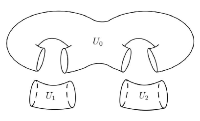
Figure 1.

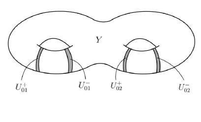
Figure 2.

Define a fundamental group action $\kappa\colon\pi_{1}(Y,\ast)\to\mathrm{Diff}^{\omega}_{+}(S^{1})$ by letting $\kappa(\alpha_{1})=f_{1}$, $\kappa(\alpha_{2})=f_{2}$, and $\kappa(\beta_{1})=\kappa(\beta_{2})=\mathrm{id}_{S^{1}}$ for generating loops $\alpha_{1},\alpha_{2},\beta_{1}$, and $\beta_{2}$ (see Figure 3).

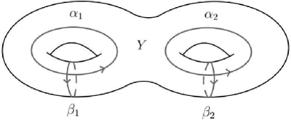
Figure 3.

By considering extending a domain of $f_{1}$ and $f_{2}$ along the unit circle, one obtains a non-singular complex surface $X$ which has a Levi-flat hypersurface $M$ constructed by suspension of $\kappa$. Let $\pi\colon M\to Y$ be the projection and $P$ be a holomorphic submersion as in §1. For the good system of local functions $\{(V_{j},(z_{j},w_{j}))\}$ of $\sigma>0$ over $\{Y,\mathcal{U},\kappa,X,P\}$, we define the transversal transition on each $V_{01}^{+},V_{01}^{-},V_{02}^{+}$, and $V_{02}^{-}$, where $\{V_{0j}^{\epsilon}\}_{\epsilon=+,-,\ j=1,2}$ are the connected components of the intersection $M_{0j}=M_{0}\cap M_{j}=\pi^{-1}(U_{0})\cap\pi^{-1}(U_{j})\ (j=1,2)$. Denote by $w_{j}=f_{j0}^{+}(w_{0})=f_{j}(w_{0})$ the transition on $V_{0j}^{+}$ and by $w_{j}=f_{j0}^{-}(w_{0})=w_{0}$ the transition $V_{0j}^{-}$ for each $j=1,2$. Then, the Laurent expansions for transition functions are written as below:

$$\log\frac{f_{j0}^{+}(w_{0})}{w_{0}} =\log\frac{f_{j}(w_{0})}{w_{0}}\equiv\alpha_{j0}^{+}+\sum_{n\neq 0}b_{j0|n}^{+}w_{0}^{n},$$

$$\log\frac{f_{j0}^{-}(w_{0})}{w_{0}} =\log\frac{\mathrm{id}(w_{0})}{w_{0}}\equiv\alpha_{j0}^{-}\equiv 0.$$

In this situation, since $U_{0}\cap U_{1}\cap U_{2}=\emptyset$, any Čech 1-cochain over $Y$ satisfies 1-cocycle condition. Therefore one obtains

$$N=[\alpha(\{(V_{j},(z_{j},w_{j}))\})]=[\{(U_{0j}^{+},e^{\alpha_{j0}^{+}}),(U_{0j}^{-},1)\}_{j=1,2}]\in\check{H}^{1}(\mathcal{U},\mathrm{U}(1))$$

and

$$[b_{n}(\{(V_{j},(z_{j},w_{j}))\})]=[\{(U_{0j}^{+},b_{j0|n}^{+}),(U_{0j}^{-},0)\}_{j=1,2}].$$

Proposition 4.1.

Let $f_{1}$, $f_{2}$, $Y$, $\mathcal{U}$, $\kappa$, $X$, and $P$ be as above and $\{(V_{j},(z_{j},w_{j}))\}_{j=0,1,2}$ be the good system of local functions of width $\sigma$. If the followings hold, then $f_{1}$ and $f_{2}$ are simultaneous linearizable.
$(i)$ The unitary flat line budle $N$ over $Y$ satisfies $(C_{0},\mu,K)$-Diophantine condition with the constant $K=K(Y,\mathcal{U})$ obtained by Theorem 2.6.
$(ii)$

$$\max_{j=1,2}\sup_{e^{-\sigma}<|p|<e^{\sigma}}\left|\sum_{n\neq 0}b_{j0|n}^{+}p^{n}\right|<\min\left\{\eta_{0},\ \frac{\eta_{0}^{\mu+1}}{(1+e^{\sigma})C_{1}\mu}\right\}$$

for the constant $\eta_{0}\in(0,\min\{\pi,(1-\mu^{-\frac{1}{\mu+1}})\frac{\sigma}{4}\})$ and the constant $C_{1}$ which depends only on $\sigma,C_{0}$ and $\mu$.
$(iii)$ The 1-cohomology group $[b_{n}(\{(V^{\prime}_{j},(z_{j},w^{\prime}_{j}))\})]$ is cohomologous to $0$ for any good system of local functions $\{(V^{\prime}_{j},(z_{j},w^{\prime}_{j}))\}$ which satisfies $[\alpha(\{(V^{\prime}_{j},(z_{j},w^{\prime}_{j}))\})]=N$.

Proof. From Theorem 1.2, the system $\{Y,\mathcal{U},\kappa,X,P,\{(V_{j},(z_{j},w_{j}))\},\sigma\}$ is linearizable. Then, there exist the functions of retaking coordinates $\psi_{j}(u_{j})=w_{j}\ (j=0,1,2)$ and the good system of local function $\{(V^{\prime}_{j},(z_{j},u_{j}))\}_{j=0,1,2}$ whose transition is the linear map $u_{j}=e^{\alpha_{j0}^{\epsilon}}u_{0}$ for each $\epsilon=+,-$ and $j=1,2$. One obtains the following relations:

$$(\psi_{j}^{-1}\circ f_{j0}^{\epsilon}\circ\psi_{0})(u_{0})=e^{\alpha_{j0}^{\epsilon}}u_{0}.$$

Therefore we obtain the followings for each $j=1,2$:

$$(\psi_{j}^{-1}\circ f_{j}\circ\psi_{0})(u_{0})=e^{\alpha_{j0}^{\epsilon}}u_{0}$$

$$(\psi_{j}^{-1}\circ\psi_{0})(u_{0})=u_{0}.$$

Hence, one can check $(\psi_{0}^{-1}\circ f_{j}\circ\psi_{0})(u_{0})=e^{\alpha_{j0}^{+}}u_{0}$ for each $j=1,2$. That is simultaneous linearization of $f_{1}$ and $f_{2}$. Since $f_{j}$ is conjugated to the rotation $w\mapsto e^{\alpha_{j0}^{+}}w$, $\alpha_{j0}^{+}\equiv 2\pi\sqrt{-1}\rho(f_{j})\ (\mathrm{mod}\ 2\pi\sqrt{-1}\,\mathbb{Z})$ holds, where $\rho(f_{j})$ is the rotation number of $f_{j}$. ∎

5. Discussion

In this paper, we considered a function $f\in\mathrm{Diff}^{\omega}_{+}(S^{1})$ which has the Laurent expansion

$$\log\frac{f(w)}{w}=\alpha+\sum_{n\neq 0}b_{n}w^{n}.$$

Comparing the condition of main theorem with the assumption in Arnol’d’s linearization theorem, we should check a relation of the constant term of Laurent expansion as above and the rotation number of $f$. As is seen the example in §4, sometimes $\alpha$ turns out to be equal to $2\pi\sqrt{-1}\rho(f)$ modulo $2\pi\sqrt{-1}\mathbb{Z}$.

Question 5.1.

Assume that $\alpha$ is a constant term Laurent expansion of $\displaystyle{\log\frac{f(w)}{w}}$. Then, will $e^{\alpha}=e^{2\pi\sqrt{-1}\rho(f)}$ always hold?

Acknowledgment. The author would like to thank Takayuki Koike for fruitful comments. This work was partly supported by Osaka Central Advanced Mathematical Institute: MEXT Joint Usage/Research Center on Mathematics and Theoretical Physics JPMXP0619217849.

Appendix A Complement of Proposition 3.6

In this part, we will show the consequence of checking the well-definedness of the map $\psi_{k,m}^{-1}$. In what follows, we use the notation in proof of Lemma 3.9. Let $\Psi_{k,m}$ be a lift of the map $\psi_{k,m}|_{S^{1}}$. For a given point $w_{0}\in V_{k,m}(\sigma_{m}-\eta_{m})$, let $\widetilde{w}_{0}$ be a point in $B(\sigma_{m}-2\eta_{m})\coloneqq\{|\operatorname{Im}\,z|<(\sigma_{m}-2\eta_{m})/2\pi\}$ which satisfies $e^{2\pi\sqrt{-1}\widetilde{w}_{0}}=w_{0}$. We define a domain $D\subset\mathbb{C}$ by

$$D=\left\{z\in\mathbb{C}\ ;|\operatorname{Im}\,z|<\frac{\sigma_{m}-\eta_{m}}{2\pi},|\operatorname{Re}\,z-\operatorname{Re}\,\widetilde{w}_{0}|<\frac{1}{2}\right\}$$

(see Figure 4). We define holomorphic functions $g_{1},g_{2}$ on a neighborhood of $D$ by

$$g_{1}(z)=z-\widetilde{w}_{0}$$

$$g_{2}(z)=\Psi_{k,m}(z)-z$$

Lemma A.1.

For any $z\in\partial D$, $|g_{1}(z)|>|g_{2}(z)|$ holds.

Proof. One has

$$|g_{1}(z)|\geq\min\left\{\frac{1}{2},\ \frac{1}{2\pi}\eta_{m}\right\}.$$

From the definition, $\{\eta_{m}\}$ is monotonically decreasing. Thus, one obtains

$$\frac{1}{2\pi}\eta_{m}<\frac{1}{2\pi}\eta_{0}<\frac{1}{2}$$

under the assumption $\eta_{0}<\pi$. Considering the relation

$$\Psi_{k,m}(z)=z+\frac{1}{2\pi\sqrt{-1}}\widehat{\psi}_{k,m}(e^{2\pi\sqrt{-1}z}),$$

one has

$$|g_{2}(z)|=\frac{1}{2\pi}\sup_{z\in\partial D}|\widehat{\psi}_{k,m}(e^{2\pi\sqrt{-1}z})|<\frac{1}{2\pi}\eta_{m}.$$

Therefore, $\displaystyle{|g_{1}(z)|\geq\frac{1}{2\pi}\eta_{m}>|g_{2}(z)|}$ holds. ∎

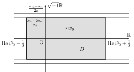
Figure 4. The domain $D$ is independent of the imaginary part of $\widetilde{w}_{0}$

Proposition A.2.

Let $S^{1}$ be the unit circle. Then $\psi_{k,m}^{-1}(S^{1})=S^{1}$ holds.

Proof. Suppose that there exists a point $a\in\psi_{k,m}^{-1}(S^{1})\backslash S^{1}$. Since the map $\psi_{k,m}$ is one-to-one on $S^{1}$ and has no critical point on $V_{k,m}(\sigma_{m}-\eta_{m})$, there exists a positive constant $\varepsilon>0$ such that $\psi_{k,m}|_{V_{k,m}(\varepsilon)}$ is isomorphism to the image and $a\notin V_{k,m}(\varepsilon)$ holds. Considering

$$|\log|\psi_{k,m}(a)|-\log|a||<\eta_{m},$$

one obtains that $a\in V_{k,m}(\eta_{m})$ holds. Thus, it is sufficient to consider the case of $\eta_{m}<\varepsilon$. In what follows, suppose that $a\in V_{k,m}(\eta_{m})\backslash V_{k,m}(\varepsilon)$. Let $\mathscr{C}$ be the connected component of $\psi_{k,m}^{-1}(S^{1})$ which has $a$. Recall that each connected component of $\psi_{k,m}^{-1}(S^{1})$ is real $\mathcal{C}^{\infty}$ curve in $V_{k,m}(\eta_{m})\backslash V_{k,m}(\varepsilon)$.

Figure 5. The thin annulus along $S^{1}$ is $V_{k,m}(\varepsilon)$. Considering the reflection principle, without loss of generality, we may assume that $\mathscr{C}$ lies inside $V_{k,m}(\varepsilon)$.

Then, one can find out that $\mathscr{C}$ is a Jordan curve in $V_{k,m}(\eta_{m})\backslash V_{k,m}(\varepsilon)$. Suppose that $\mathscr{C}$ lies inside of $S^{1}$ (see Figure 5). Denote by $\Omega$ the region enclosed by the curve $\mathscr{C}$. In this case, the region $\Omega$ satisfies $\Omega\cap\Delta(e^{-\eta_{m}})=\emptyset$ or $\Omega\supset\Delta(e^{-\eta_{m}})$, where $\Delta(e^{-\eta_{m}})$ is the circle around the origin with radius $e^{-\eta_{m}}$. In the former case, consider the harmonic function $h(w)=\log|\psi_{k,m}(w)|$. It will contradict that $\psi_{k,m}$ has no critical point. In the letter case, it is sufficient to consider the function $h$ on $\Omega\backslash\overline{\Delta(e^{-\eta_{m}})}$. ∎

From Lemma A.1, applying Rouché’s theorem, one finds that $\Psi_{k,m}(z)=\widetilde{w}_{0}$ and $\Psi_{k,m}(z)=z$ have the same number of zeros in $D$. Considering the case of $w_{0}\in S^{1}$ (i.e. $\operatorname{Im}\,\widetilde{w}_{0}$ = 0), we obtain $\#\{D\mid\Psi_{k,m}(z)=z\}=\#\{D\mid\Psi_{k,m}(z)=\widetilde{w}_{0}\}=1$. Remark that the domain $D$ is defined independently of $\operatorname{Im}\,\widetilde{w}_{0}$. Therefore, for arbitrary $|\operatorname{Im}\,\widetilde{w}_{0}|<\frac{\sigma_{m}-2\eta_{m}}{2\pi}$, one finds $\#\{D\mid\Psi_{k,m}(z)=\widetilde{w}_{0}\}=1$. Consequently one can define $\psi^{-1}_{k,m}$ on $V_{k,m}(\sigma_{m}-2\eta_{m})$.

References

- [A] V. I. Arnold, Small denominators. I: On the mappings of the circumference onto itself, Isv. Akad. Nauk, Math series , 25, 1, (1961), p. 21–96. Transl. A. M. S, 2nd series, 46, p. 213–284.
- [CG] Lennart Carleson and Theodore W. Gamelin, “COMPLEX DYNAMICS”, Universitext: Tracts in Mathematics Springer–Verlag 1993.
- [KH] Anatole Katok and Boris Hasselblatt, “Introduction to the Modern Theory of Dynamical Systems”,Cambridge University PressEncyclopedia Math. Appl., 54, Cambridge Univ. Press, 1995.
- [KU] T. Koike and T. Uehara, A gluing construction of K3 surfaces, arXiv:1903.01444.
- [S] C. L. Siegel, Iteration of analytic functions, Ann. Math. 43, 607–612 (1942).
- [SM] C.L. Siegel and J.K. Moser, “Lectures on Celestial Mechanics”, Springer-Verlag (1971).
- [U] Tetsuo Ueda, On the neighborhood of a compact complex curve with topologically trivial normal bundle, Math. Kyoto Univ., 22 (1983), 583–607.
- [Y] Jean-Crhistophe Yoccoz, “Analytic linearization of circle diffeomorphisms Dynamical systemsand small divisors”(Cetraro, 1998), 125-173, Lecture Notes in Math., 1784, Fond.CIME/CIME Found. Subser., Springer, Berlin, (2002).