PICASSO: Unleashing the Potential of GPU-centric Training for Wide-and-deep Recommender Systems

Abstract

The development of personalized recommendation has significantly improved the accuracy of information matching and the revenue of e-commerce platforms. Recently, it has two trends: 1) recommender systems must be trained timely to cope with ever-growing new products and ever-changing user interests from online marketing and social network; 2) state-of-the-art recommendation models introduce deep neural network (DNN) modules to improve prediction accuracy. Traditional CPU-based recommender systems cannot meet these two trends, and GPU-centric training has become a trending approach. However, we observe that GPU devices in training recommender systems are underutilized, and they cannot attain an expected throughput improvement as what it has achieved in Computer Vision (CV) and Neural Language Processing (NLP) areas. This issue can be explained by two characteristics of these recommendation models: First, they contain up to a thousand of input feature fields, introducing fragmentary and memory-intensive operations; Second, the multiple constituent feature interaction submodules introduce substantial small-sized compute kernels. To remove this roadblock to the development of recommender systems, we propose a novel framework named PICASSO to accelerate the training of recommendation models on commodity hardware. Specifically, we conduct a systematic analysis to reveal the bottlenecks encountered in training recommendation models. We leverage the model structure and data distribution to unleash the potential of hardware through our packing, interleaving, and caching optimization. Experiments show that PICASSO increases the hardware utilization by an order of magnitude on the basis of state-of-the-art baselines and brings up to 6$\times$ throughput improvement for a variety of industrial recommendation models. Using the same hardware budget in production, PICASSO on average shortens the walltime of daily training tasks by 7 hours, significantly reducing the delay of continuous delivery.

I Introduction

Figure 1: The trend of WDL approaches from the perspective of a business task in Alibaba. The average GPU utilization of these models is collected from the training workloads by an in-house optimized Tensorflow in PS training strategy. The statistics show that along with the performance improvement, training WDL models does not take full advantage of the GPU resources by the canonical training frameworks (which reach 95%+ GPU utilization when training CV or NLP models of same scale).

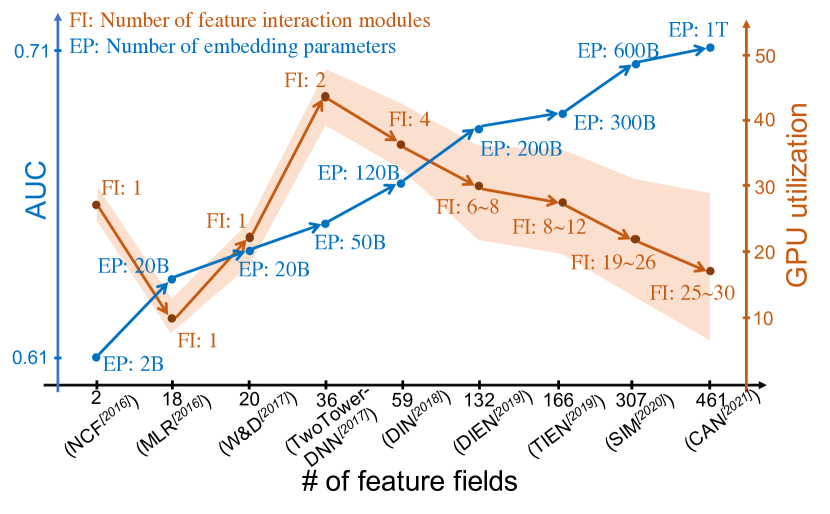
Recommender systems have nowadays become the key for higher revenue, user engagement, and customer retention on social network and E-commerce platforms. To cope with the explosive data growth, recommender systems are quickly evolving from collaborative filtering [1] (CF) to deep neural network (DNN) models and consistently improving the task accuracy, as shown in Fig. 1. Starting from Google’s Wide&Deep [2], the innovation of industrial-scale recommendation models [3, 4, 5, 6, 7, 8] follows two trends: 1) the embedding layer becomes wider, consuming up to thousands of feature fields [6]; 2) the feature interaction layer is going deeper [6, 7, 8] by leveraging multiple DNN submodules over different subsets of features. We denote these models as Wide-and-Deep Learning (WDL) Recommendation Models.

The industrial WDL models must be periodically re-trained to reflect user interest drift and new hot spots timely and accurately. Hence, high training throughput is critical for WDL models to catch up streaming data and reduce the latency of continuous delivery [9]. Training the state-of-the-art WDL models via Parameter Server (PS) [10] on a large-scale distributed CPU cluster is time-consuming owing to insufficient computation capability to accomplish deep feature interactions. Recent work, represented by Facebook’s TorchRec, Baidu’s PaddleBox [11], and NVIDIA’s HugeCTR prefer a GPU-centric synchronous training framework on WDL workloads because high-end NVIDIA GPU (e.g., NVIDIA Tesla V100) has a 30x higher single precision FLOPS over Intel CPU . Most of these efforts do improve the training throughput by leveraging GPU devices. However, we observe substantial hardware underutilization (e.g., measured GPU utilization) along with the growing number of feature fields and feature interaction modules, as illustrated in Fig. 1. This implies that the WDL training workloads are far from achieving the peak performance of hardware, and a further acceleration shall be anticipated. Although customizing hardware for a specific WDL workload pattern could be an option [12], there are following concerns: 1) We have various WDL designs owning markedly different workload patterns (e.g., the number of feature fields, the submodules of feature interaction layer), and new WDL models are emerging monthly; 2) For public cloud usage, commodity hardware is preferred for the sake of budget and elasticity. Thus, we raise two questions of What causes the hardware underutilization issue in training WDL models?, and Can we address this issue from software system’s perspective? We conduct a systematic analysis (detailed in §II) across a variety of WDL workloads and obtain implications as follows:

1. WDL model training has fragmentary operations within embedding and feature interaction layers because of the massive number (up to thousands) of feature fields, which brings in a non-trivial overhead of launching operations (e.g., issuing a CUDA kernel to CUDA streams) and hardware underutilization.

2. The embedding layer of WDL model mainly consists of memory-intensive and communication-intensive operations (in distributed environments), while the feature interaction and multi-layer perceptron (MLP) own computation-intensive operations. The computing resource would be underutilized in processing the large volume of embedding parameters and leads to a pulse-like GPU usage.

We then propose a novel framework with Packing, Interleaving and Caching Augmented Software System Optimization (PICASSO) to answer the above two questions. First, we create fine-grained embedding feature groups. Operations within the same group are packed to reduce the number of fragmentary operations; Second, operations from distinct groups are interleaved from both of data level and kernel level to improve hardware utilization; Third, we develop a data distribution-aware caching mechanism leveraging the large volume of DRAM and the high bandwidth of GPU device memory.

Evaluation shows that PICASSO significantly improves the GPU utilization during training a variety of industrial WDL models, and it accelerates the throughput by an order of magnitude compared to state-of-the-art generic training frameworks. PICASSO has been deployed in our in-house training cluster, appearing as XDL2 within Alibaba and HybridBackend in AliCloud. The delay to continuous delivery is decreased from 8.6 hours to 1.4 hours on average, which is unprecedented inside Alibaba and instructive to the community. We summarize the main contributions of this paper as follows:

1. We analyze the hardware underutilization and reveal the cause when training WDL models by GPU-centric synchronous frameworks.

2. We propose PICASSO that resolves the underutilization issue with a software-system approach that is applicable to commodity hardware.

3. We build a system that sustains our daily production workloads with up to a trillion parameters and petabytes of training data, achieving 6x training performance speedup on average without increasing the budget. PICASSO has been released for public cloud usage .

Figure 2: A Standard architecture of WDL, 1) The embedding layer ingests multiple fields of features (as opposed to NLP tasks with only one field of “word”), adopts various hashing or numerical operations, and queries embedding (in various dimension) from memory; 2) The feature interaction layer processes the fetched feature embeddings through a number of feature interaction modules; 3) the outputs of the modules are concatenated and fed to the multi-layer perception (MLP) for yielding final predictions.

II Implication from Analyzing Workloads

II-A Architecture of WDL Models

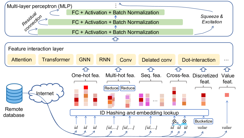
WDL models share a typical architecture as shown in Fig. 2: Data Transmission Layer processes streamed training data in the form of categorical feature identity (ID) as well as dense feature vectors. Categorical feature IDs usually have a varying length (i.e., multi-hot or non-tabular data), and they can reach up to tens or hundreds of MBytes within a batch. Normally, the data is stored in remote databases and requires a transmission via Ethernet;

Embedding Layer projects a high-dimensional feature space of sparse categorical features to a low-dimensional embedding feature space. The embedding parameters are represented by dense vectors named feature embedding, and they are stored in DRAM in the form of embedding tables. Each feature embedding can be queried by its categorical feature ID to get trained in WDL. Since a large volume of feature embeddings would be queried from DRAM per training batch, the embedding layer is dominated by memory-intensive operations.

Figure 3: Distribution of categorical feature IDs across representative WDL datasets.

Figure 4: Low-level projection of the standard architecture of WDL models: the multiple feature fields and constituent feature interaction modules would duplicate a large number of operations in the computation graph.

Feature Interaction Layer would first organize feature embeddings from the embedding layer into several groups. Each group applies an individual feature interaction module, such as GRU [13] and Transformer [14], to extract useful information from intra-group feature embeddings. The outputs of the constituent feature interaction modules are then concatenated to form a final output of the feature interaction layer. There could be tens of constituent feature interaction modules to engage different subsets of feature embedding, yielding up to hundreds of thousands of operations.

MLP builds fully-connected layers to provide final predictions by the training data of a batch. MLP also contains computation-intensive architectural units such as batch normalization [15] and residual connection [16]. It is worth noting that the accuracy loss is usually intolerable in many business scenarios. Thus, generic acceleration strategies (e.g., half-precision, quantized pruning [17], gradient staleness) may only apply to a fraction of WDL models.

II-B Data Distribution in WDL Workload

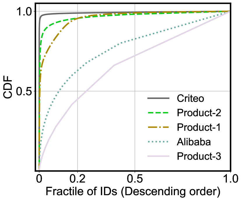
The categorical feature IDs of each feature field are usually skewed or non-uniformly distributed. We investigate the data distribution of five representative WDL datasets (statistics are listed in Tab. II) and Fig. 4. When being sorted in a descending order by frequency, 20% of IDs will cover 70% by average and up to 99% of the training data. Therefore, it is beneficial to cache frequently accessed data when training WDL models.

II-C Distributed Training Strategies of WDL Model

In general, three types of training strategies are adopted in training WDL models in a GPU-centric distributed system:

Parameter Server (PS) Strategy [10] is still the de facto training strategy applied in industry, where training data is partitioned across multiple worker nodes while model parameters are partitioned across multiple server nodes. Worker nodes would pull down model parameters from server nodes and train them by using local partitioned training data; By the end of each iteration, worker nodes would push up corresponding gradients back to server nodes asynchronously to update the parameters.

Data-parallel (DP) Strategy is the default distributed training strategy by frameworks such as Tensorflow [18] and PyTorch [19]. The training data is evenly partitioned across all worker nodes while the model parameters are replicated across all worker nodes. It uses a collective communication primitive named Allreduce to aggregate gradients and thus updates local replica of model parameters synchronously.

Model-parallel (MP) Strategy [20, 21] has no server nodes. Instead, it partitions and stores all parameters across multiple worker nodes. It then uses a collective communication primitive named AllToAllv to exchange data among all worker nodes synchronously.

II-D Characterization of WDL Workload

We first conduct a low-level projection of WDL workloads to the underlying hardware, and we then summarize three representative workload patterns.

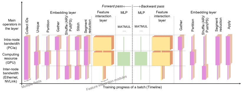
Each WDL layer consists of a set of operators from the algorithmic perspective. An operator is normally implemented as a kernel in programs, and their invocations during the training are referred as the operations. The execution of an operation requires various hardware resources. Fig. 4 illustrates a low-level projection of a standard WDL model trained within a distributed system with respect to three types of hardware resources: intra-node bandwidth (e.g, DRAM and PCIe bandwidth), computing resource (e.g., GPU Streaming Multiprocessors (SM)), and inter-node bandwidth (NVLink and Ethernet bandwidth). In distributed training of WDL models, the embedding layer mainly consists of the following operators: Unique (eliminate redundant categorical feature IDs to reduce memory access overhead), Partition (partition categorical feature IDs into local IDs and remote IDs), Gather (query local IDs from embedding tables), Shuffle (communicate remote worker nodes to fetch feature embeddings belonging to remote IDs), Stitch (concatenate locally queried feature embeddings and remotely fetched feature embeddings), and SegmentReduction (pooling feature embedding by segments, e.g., summation of behaviour feature embeddings from the same user). The embedding layer has a majority of operators bounded by a dominant type of hardware resource (e.g., the Shuffle operator is bounded by inter-node bandwidth). The feature interaction layer and MLP have operators mainly bounded by computation resources. Similarly, the backward pass can be treated as a mirror image of the forward pass. In a synchronous GPU-centric training system, this low-level projection indicates that the hardware resource usage is sporadic, which implies that, at a time, the training would be bounded by one type of hardware resource while the other types of resource are underutilized.

This projection reflects three characteristics of WDL workloads compared to CV and NLP workloads.

• Embedding layer and feature interaction layer involve a massive number of small-sized operations (i.e., embedding of single feature field could involve hundreds of operations, and WDL workload would have to process up to thousands of feature fields), which has a significant launch overhead.

• The invocations of the same operator from the embedding layer by different feature fields would race for the same type of hardware resource at a time, which bounds the throughput when the hardware resource is relatively strained (e.g., PCIe bandwidth between CPU and GPU).

• The skewed data distribution as described in §II-B would cause unbalanced hardware resource usage across worker nodes in distributed systems, which shall compromise the throughput during synchronous training.

Figure 5: Worker-side breakdown of the three WDL models by PS and MP strategies (“exposed” indicates the period when the operation blocks all the others).

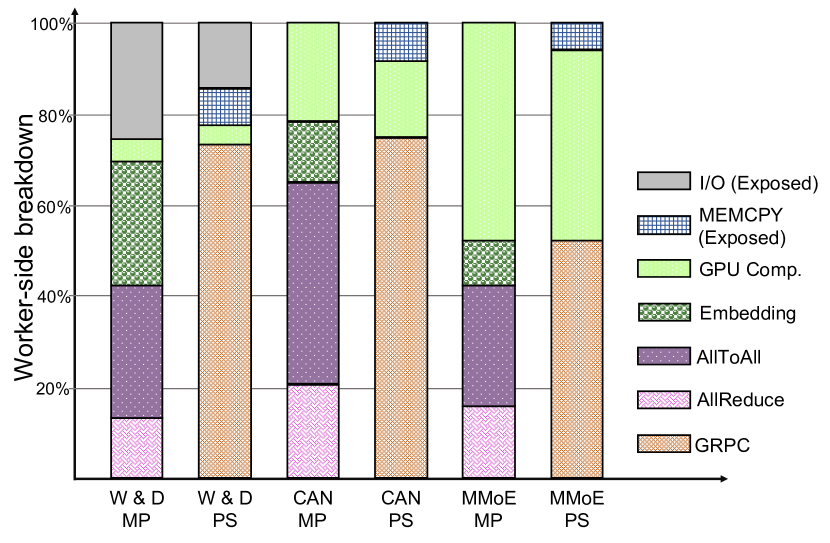
We probe into the statistics of WDL workloads from a cluster of NVIDIA Tesla V100s (“EFLOPS” in Tab. I) at Alibaba Cloud (composed of commodity hardware devices, as specified in [22]). The models are implemented by Tensorflow under either PS strategy or MP strategy as introduced in §II-C. We observe three representative patterns from the profiling and worker-side performance breakdown, as shown in Fig. 5.

• I/O&Memory Intensive Workload. WDL models represented by W&D [2] have substantial data transmission and embedding lookup operations, where the I/O may not be fully overlapped by the other procedures, as shown in Fig. 5. I/O&Memory intensive models emerge along with the prosperity of feature engineering and transferable pretrained embedding, where massive feature fields should be tackled to achieve the best accuracy. Even with I/O optimization, the exposed I/O and memory access still occupy around 20% of the total training walltime in Fig. 5.

• Communication Intensive Workload. This type of workload spends most of the time in communication-related operations. The large volume of communication from fetching remote high-dimensional embedding features as well as the frequent parameter exchange from high-order cross features cause severe communication overhead in distributed WDL workloads. We take CAN [8] for instance, which is recently derived from DIN [4] and DLRM [23]. CAN contains a combination of feature interaction modules over a substantial number of feature fields, and therefore it brings up an extensive communication overhead by around 60% in MP mode and 70% in PS mode as shown in Fig. 5.

• Computation Intensive Workload. Some WDL models are throttled by computation operations, since deep and complex WDL models benefit from the advancement in the domain of CV and NLP. A variant of MMoE [24], which is derived from canonical DIN [4] and owns 71 experts at MLP, serves for scenario-aware CTR prediction in our business. In Fig. 5, MMoE spends about 50% of the training time in arithmetic calculations. In practice, computation-intensive WDL models tend to work for scenarios of multiple sub-tasks [25] (e.g., multi-objective learning, meta-learning), super-complicated computation [26] (e.g., extremely-deep network over a number of feature fields), and multi-modal co-training [27].

III System Design of PICASSO

In this section, we first introduce the overall architecture of PICASSO, which accommodates the hardware topology of GPU-centric training cluster and thus allows a hybrid distributed training strategy for WDL models. Second, we introduce a three-fold key idea of accelerating training by improving hardware utilization.

III-A Hybrid Distributed Training Strategy

Figure 6: PICASSO allows the hybrid strategy of MP and DP, where embedding parameters are partitioned across PICASSO-Executors (MP), and dense parameters are replicated across PICASSO-Executors (DP). Besides, canonical DP and MP are also supported by PICASSO.

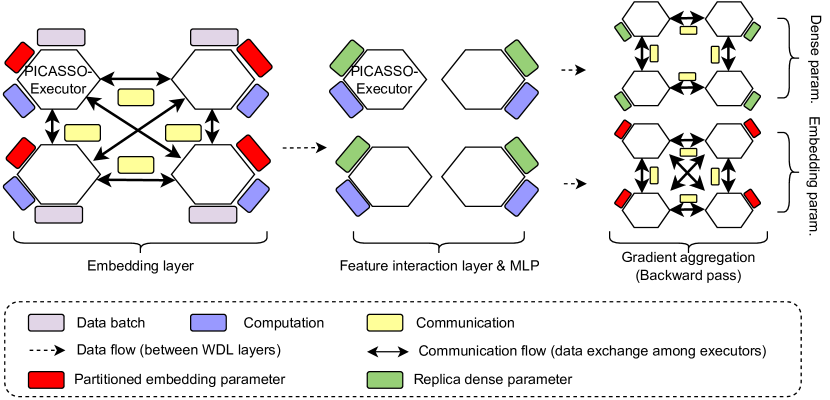
We propose the architecture of PICASSO in Fig. 6, which is designed for GPU-centric clusters. One such cluster usually consists of multiple homogeneously configured machines (cluster node), and each machine instead has a heterogeneous architecture, including processors (e.g., Intel CPU), accelerators (e.g., NVIDIA GPU), and the uncore system (e.g., DRAM). In addition, there are interconnects like PCIe and NVLink among components within a machine, and all these machines are further connected through Ethernet as a distributed system. Correspondingly, PICASSO sets up multiple PICASSO-Executors, which are mapped to different machines in the cluster. Each PICASSO-Executor has heterogeneous hardware resource: 1) GPU Stream Multiprocessor (SM) and CPU physical cores as computation resource; 2) hierarchical memory subsystem made of GPU device memory, DRAM, Intel Persistent Memory, and SSD (if accessible) as memory storage resource; 3) hierarchical interconnects like NVLink, PCIe, InfiniBand, and Ethernet as communication resource.

With this architecture, PICASSO can customize hybrid distributed training strategies for different layers within WDL model as follows:

• The embedding layer has a tremendous volume of embedding parameters, and it adopts a model-parallel (MP) strategy. The embedding parameters are partitioned across all PICASSO-Executors and stored within the hierarchical memory subsystem. The parameters are exchanged synchronously among PICASSO-Executors via the AllToAllv collective communication primitive.

• Feature interaction layer and MLP have a much smaller volume of parameters than the embedding layer. We adopt a data-parallel (DP) strategy for those two layers, where the parameters are replicated across all PICASSO-Executors and aggregated via the Allreduce primitive.

III-B Packing

Figure 7: Illustration of packing optimization: a) Without packing, looking up feature embedding from three embedding tables requires a total of 18 operators; b) By D-packing and K-packing, PICASSO reduces the total number of operators to 4 packed operators.

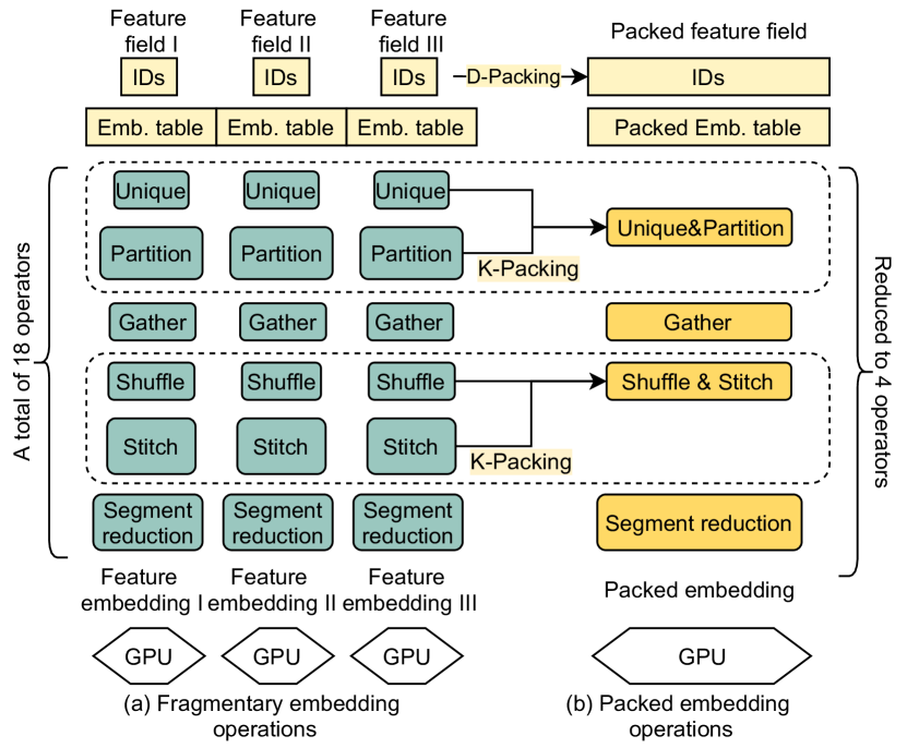
To address the fragmentary operations as described in §II-D, we propose a Packing method that effectively reduces the number of operations from two aspects:

Figure 8: (a) D-Interleaving starts from MLP to eliminate GPU device memory capacity bounds; (b) D-Interleaving starts from the embedding layer to reduce overhead. (c) K-Interleaving the packed and non-packed embedding operations on different hardware resource.

Data-Packing (D-Packing). When categorical feature IDs from different feature fields are fed into the same operator within the embedding layer, PICASSO combines categorical feature IDs into a single packed ID tensor. Thus, we can launch a single operation (named packed operation) to process the packed data, which fits into the Single-Instruction-Multiple-Data (SIMD) programming paradigm [28] of NVIDIA GPU devices. Also, it significantly reduces the overhead of launching a massive number of operations onto GPU devices.

In addition, a naive strategy of packing up all categorical feature IDs into a single tensor may cause severe throughput issues. For instance, industrial-scale recommender systems usually implement embedding tables by using a hashmap to accommodate the growing amount of feature embedding. A massive number (million-level) of concurrent querying requests shall suffer from the low-level locks of a hashmap. Therefore, we pack up categorical feature IDs when their embedding tables share the same feature dimension. Thus, we obtain packed operations with the number proportional to that of distinct feature dimensions. Nevertheless, some packed operations may still encounter too many concurrent queries to compromise the throughput of the hashmap due to skewed data distribution and large feature dimensions. We propose a method to evaluate the execution cost by estimating the parameter volume (the number of floats) within packed operations as shown in Equation 1.

$$\text{CalcVParam}(T)=N\sum_{t\in T}(t_{\text{dim}}\sum_{\text{ID}\in t}\text{ID}_{\text{freq}}),$$ (1)

where $N$ refers to the total number of categorical feature IDs, $T$ refers to a packed embedding table, $t_{\text{dim}}$ denotes the feature dimension of an embedding table, and $\text{ID}_{\text{freq}}$ refers to the frequency of a categorical feature ID. $N$ and $\text{ID}_{\text{freq}}$s would be obtained from the statistics in the warm-up iterations. If a packed operation has a high $\text{CalcVParam}(T)$ above average, we shall further evenly split it into multiple shards. For instance, suppose that we have one packed operation for all embedding tables with a feature dimension of 8 and the data distribution is uniform. For embedding tables with a dimension of 32, we will create four shards of packed operations, each with a quarter of these embedding tables.

Kernel-Packing (K-Packing). Kernel fusion is already a widely adopted optimization for deep learning systems. There are mainly two approaches: 1) hand-written huge kernels; 2) compilation-based code generation. Huge kernels, such as fusing the whole embedding layer into a single CUDA kernel, would miss the opportunity of interleaving operations bounded by distinct hardware resources (see details in §III-C). Compilation-based code generation relies on static input and output shapes from each operator to infer the suitable sizes for generated kernels. However, categorical feature IDs induce dynamic operator shapes that disrupt the efficiency of compilation techniques like Tensorflow XLA. In contrast, our kernel-packing evaluates all kernels by their hardware resource utilization, and they are grouped into computation-intensive kernels, memory-intensive kernels, and communication-intensive kernels. We only fuse up kernels from the same kernel group and leave opportunities for interleaving their execution across different kernel groups.

Fig. 7 illustrates the process of our packing optimization. Categorical feature IDs are first grouped together (i.e., D-Packing). Each group of categorical feature IDs is fed into a fused kernel (i.e., K-Packing) named Unique&Partition to eliminate memory access and data communication from redundant IDs. The categorical feature IDs would be fetched from their local partition of embedding tables. We then develop another fused kernel named Shuffle&Stitch to fulfill a stitched output of the shuffle kernel and remove the explicit stitch kernel.

III-C Interleaving

After applying the Packing optimization, we further develop two types of Interleaving optimization to improve utilization across different hardware resources.

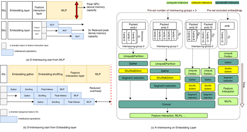
Data-Interleaving(D-Interleaving): When WDL model is trained with large batch sizes (e.g., tens of thousand), operations would suffer from various hardware bounds. For instance, the footprint of GPU device memory from intermediate tensors (the so-called feature map in Tensorflow) is proportional to the data batch size. Because the capacity of GPU device memory is restricted (e.g., 32GBytes in NVIDIA Tesla V100), large batch size is likely to cause an out-of-memory (OOM) issue and crash the training. However, large batch size is usually desired for both high accuracy and throughput in WDL training. Therefore, PICASSO adopts a micro-batch-based data interleaving (D-interleaving) approach that allows users to slice and interleave workloads starting from a specified layer of WDL models. To address the OOM issue of GPU device memory, we can divide the output embedding of feature interaction layer into several micro batches and apply D-Interleaving on MLP, where the peak GPU device memory usage can be amortized as shown in Fig. 8 (a). Also, we can divide categorical feature IDs into several micro batches and apply D-Interleaving to the rest of the training Fig. 8 (b). By default, we evenly divide data into micro batches to attain a load balancing, and the micro-batch size can be estimated by:

$$\text{BS}_{\text{micro}}=\min_{\text{op}\in\text{layer}}(\text{RBound}_{\text{op}}/\text{RInstance}_{\text{op}}),$$ (2)

where $\text{BS}_{\text{micro}}$ is the estimated micro-batch size, $\text{RBound}_{\text{op}}$ denotes the bound value of an operator’s dominant hardware resource (e.g., GPU device memory capacity), and $\text{RInstance}_{\text{op}}$ denotes the cost per data instance from an operator’s dominant hardware resource. Since the shape of an operator from the embedding layer is usually dynamic, no analytical values from Equation 2 can be deduced in advance. Instead, we determine their values empirically or experimentally from warm-up iterations of training.

Kernel-Interleaving(K-Interleaving): The Packing mechanism transforms hundreds of operations into a small number of packed operations. However, the packed operations from different embedding tables still race for the same hardware resource. For instance, when all the Shuffle&Stitch operations are launched concurrently, the Ethernet bandwidth would throttle the training throughput. We propose a Kernel-Interleaving (K-Interleaving) optimization that establishes control dependencies among groups of packed operations as shown in Fig. 8. To ensure that a so-called Interleaving group would not be bounded by various hardware resources, we first determine the capacity of each interleaving group, denoted as $\text{Capacity}_{\text{g}}$, in terms of processed parameters by:

$$\text{Capacity}_{\text{g}}=\min_{\text{op}\in\text{layer}}(\text{RBound}_{\text{op}}/\text{RParam}_{\text{op}}),$$ (3)

where $\text{RBound}_{\text{op}}$ has the same definition as in Equation 2 and $\text{RParam}_{\text{op}}$ denotes the cost of training a parameter from an operator’s dominant hardware resource. Here, we simply treat the parameter volume as the cost in embedding lookup and exchange.

We could also change the number of interleaving groups by proportionally modifying $\text{Capacity}_{\text{g}}$ in PICASSO. It is worth noting that we allow users to specify a preset excluded embedding, where the packed operations have no control dependencies on the other K-Interleaving groups. For instance, when the output (feature embedding) of some operations will not be concatenated with other feature embedding for the downstream layers, K-Interleaving can advance their downstream operations.

III-D Caching

Figure 9: Gather embedding vectors (e.g., “Emb-8002”) via Cache approach upon HybridHash.

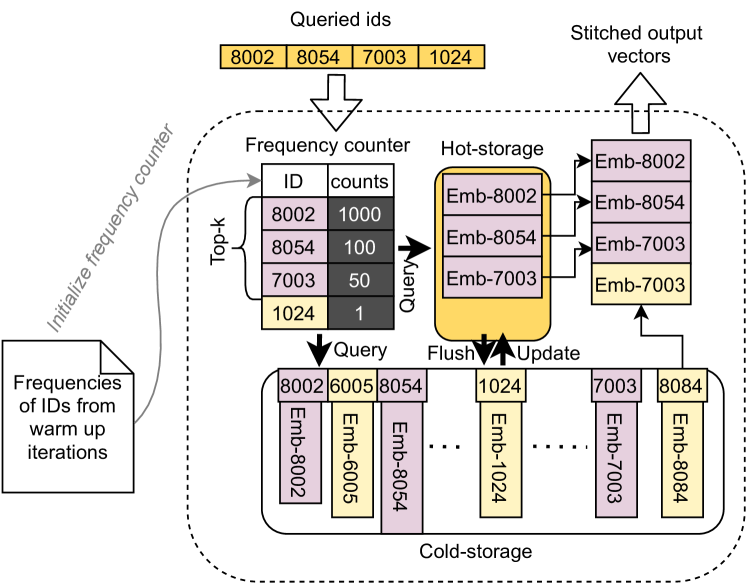
Caching is a widely applied system technique that utilizes the hierarchical memory subsystem to reduce memory access latency. However, the effectiveness of caching, i.e., the cache hit ratio, depends on multiple factors such as the data distribution and the access pattern. In §II-B, we observe that only 20% of the categorical feature IDs are being queried in a high frequency, which motivates us to propose an optimization named HybridHash. It aims to eliminate two hardware bounds: 1) The DRAM has a large capacity but is bounded by the memory access bandwidth; 2) The GPU device memory has a high bandwidth but is bounded by the limited capacity.

As shown in Fig. 9, HybridHash serves as a hashmap to store, fetch, and update embedding parameters. We refer to GPU device memory as the Hot-storage and DRAM as the Cold-storage. Unlike other GPU-based hashmap solutions, we consider Hot-storage as an expensive resource, which shall avoid any waste of its capacity. Therefore, we place the hashmap, a sparse data structure, on Cold-storage and utilize Hot-storage only as a scratchpad to store and update the frequently accessed embedding. Recall from §II-B that categorical feature IDs in WDL workload follow a certain distribution. It is reasonable to record the frequency of each queried ID from the hashmap during a predefined number of warm-up iterations. HybridHash then periodically loads the top-$k$ ($k$ would be determined by the size of Hot-storage) frequent embedding from Cold-storage to Hot-storage to retain the hottest categorical feature IDs. After the warm-up steps, the majority of ID queries are expected to hit in Hot-storage, and missed queries can be handled by Cold-storage. Note that HybridHash would place all data on Hot-storage when its capacity is found to be far beyond the total size of embedding tables during the warm-up steps. In addition, HybridHash can be extended to a multiple-level cache system, including devices like Intel’s persistent memory and SSD. The algorithm of HybridHash is shown in Algorithm 1. L9-12 depict the steps to collect statistics during the warmup iterations, L14-22 introduce the rules to get embedding, and L23-26 define the procedures to update the content in Hot-storage.

Algorithm 1 Algorithm of HybridHash

1:procedure HybridHash(IDs, itr) CStore: cold storage to hold hashmap

2:HStore: hot storage as a cache

3:FCounter: a host-side counter to record ID’s frequency

4:warmup_iters: iterations to warm up Hybridhash

5:flush_iters: flush HStore by top features in CStore every flush_iters

6:IDs: categorical feature IDs to query

7:itr: current iteration

8:     if $\text{itr}<\text{warmup\_iters}$ then

9:         for $\forall id\in\text{IDs}$ do

10:              $\text{FCounter}(id)\leftarrow\text{FCounter}(id)+1$

11:              $feat(id)\leftarrow\text{CStore}(id)$

12:         end for

13:     else

14:         for $\forall id\in\text{IDs}$ do

15:              if $id$ is found in HStore then

16:                  $feat\_hot(id)\leftarrow\text{HStore}(id)$

17:              else

18:                  $feat\_cold(id)\leftarrow\text{CStore}(id)$

19:              end if

20:              $\text{FCounter}(id)\leftarrow\text{FCounter}(id)+1$

21:         end for

22:         $feat=feat\_hot\cup feat\_cold$

23:         if $\text{itr}\%\text{flush\_iters}=0$ then

24:              $hot\_ids\leftarrow\text{top-}k(\text{FCounter})$

25:              $\text{HStore}\leftarrow\text{CStore}(hot\_ids)$

26:         end if

27:     end if

28:return $feat$

29:end procedure

IV Experiment

In this section, we conduct extensive experiments to answer the following research questions:

• RQ1: To what extent does PICASSO improve training throughput by unleashing the hardware potential compared to the state-of-the-art generic frameworks with computation optimizations?

• RQ2: How do the software system optimizations in PICASSO affect the utilization of each hardware resource?

• RQ3: How does PICASSO perform on the diversified WDL model architectures and feature fields?

IV-A Experimental Setup

We conduct the experiments on PICASSO from two aspects: 1) Benchmarking the performance of PICASSO with state-of-the-art frameworks on public datasets. 2) Evaluating the design of PICASSO by production-ready datasets and three representative models. Tab. I summarizes our testbeds, including public-accessible machines from AliCloud (Gn6e) for the performance benchmarking, as well as an on-premise cluster of Tesla-V100 (EFLOPS) for the system design evaluation.

TABLE I: Specification of testbeds (per node)

Cluster	CPU	GPU	DRAM	Network
Gn6e	Xeon 8163 (96 cores)	8xTesla V100-SXM2 (256GB HBM2)	724GB DDR4	32Gbps (TCP)
EFLOPS	Xeon 8269CY (104 cores)	1xTesla V100S-PCIe (32GB HBM2)	512GB DDR4	100Gbps (RDMA)

Testing Models and Datasets. DLRM [23] is a benchmarking model proposed by Facebook and adopted by MLPerf; DeepFM [3], derived from Wide&Deep model, is widely applied in industrial recommender systems; DIN [4] and DIEN [5] are two models training multi-field categorical data with complicated feature interaction modules. We also utilize the three representative models discussed in §II for a system-design evaluation.

For benchmarking datasets, we collect: 1) Criteo [29], a widely adopted click-through-rate (CTR) dataset by Kaggle and MLPerf [30], and 2) Alibaba[7], an open-sourced industrial-level CTR dataset. For a system-design evaluation, we use in-house production datasets at Alibaba, which has a large number of one- or multi-hot categorical features. The statistics of these datasets are depicted in Tab. II. The datasets are placed on a remote server to download via network. Following common industrial settings, the models would go through only one epoch of the entire dataset and adopt a full-precision training to avoid accuracy loss.

TABLE II: Statistics of datasets in experiments (lengths of sequential features are shown in parentheses)

Dataset	Instances	# numeric features	# sparse feature fields	Model	Emb. dim.	# of params
Criteo	4B	13	26	DLRM/ DeepFM	128	6B
Alibaba	13M	0	1,207 (7+12$\times$100)	DIN/ DIEN	4	6B
Product-1	Infinite	10	204	W&D	8$\sim$32	160B
Product-2	Infinite	0	1,834 (334+30$\times$50)	CAN	8$\sim$200	1T
Product-3	Infinite	0	584 (84+10$\times$50)	MMoE	12$\sim$128	1T

State-of-the-art Training Frameworks. We evaluate and compare the performance of PICASSO with mainstream open-sourced WDL training frameworks, including: Tensorflow-PS (abbr. TF-PS) of version 1.15 [31] with an asynchronous PS training strategy (one PS on CPU and multiple workers on GPUs). NVLink does not work in this training mode; PyTorch of version 1.8 [32] with a hybrid training strategy on WDL models with AllToAll communication (over NCCL) developed by Facebook. The embedding tables towards different feature fields are manually placed on different GPUs based on their sizes; Horovod [33] on PyTorch distributed data-parallel (DDP) mode with an Allreduce communication.

Evaluation Metrics. A group of metrics are employed in our experiments for comprehensive measurements:

• AUC is a standard CTR metric to evaluate the accuracy;

• Performance refers to the throughput of training system (instances per second per node (IPS)) and training walltime (GPU core hours);

• GPU SM Utilization is the fraction of time, when at least one warp was active on a multiprocessor, averaged over all SMs;

• Bandwidth Utilization is the measured network (PCIe / NVLink / RDMA) bandwidth.

We use NVIDIA’s DCGM [34] to inspect the metrics of device utilization on our testbeds.

Figure 10: Walltime in GPU core hours of training the four models completely by the compared training systems.

Figure 11: CDF of SM utilization of training DLRM during the entire process by the four compared systems.

Figure 12: PCIe and NVLink bandwidth consumption of training DLRM by the four compared systems.

IV-B Evaluation on Benchmarks (RQ1)

We first examine the performance of PICASSO on one Gn6e cluster node over benchmarking tasks. We tune the batch sizes for each framework’s best throughput while maintaining the models’ accuracy.

TABLE III: AUC of trained models by four training systems

	PICASSO	PyTorch	TF-PS	Horovod
DLRM	0.8025 (42K)	0.8025 (7K)	0.8024 (6K)	0.8025 (10K)
DeepFM	0.8007 (30K)	0.8007 (7K)	0.8007 (7K)	0.8007 (8K)
DIN	0.6331 (32K)	0.6329 (20K)	0.6327 (16K)	0.6329 (24K)
DIEN	0.6345 (32K)	0.6344 (16K)	0.6340 (12K)	0.6343 (24K)

Accuracy and Throughput. The AUCs, with corresponding batch sizes per GPU device, are listed in Tab. III. For DLRM and DeepFM, PICASSO achieves the same AUC with PyTorch and Horovod, which is better than the asynchronous training by TF-PS. For DIN and DIEN, PICASSO even obtains a slightly improved accuracy than the others, which is instructive for industrial practice.

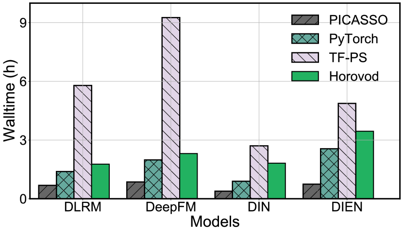
In terms of throughput, Fig. 12 records the training walltime of models by the four frameworks. TF-PS has the worst performance among the four because of extensive data exchange and PCIe congestion between server and worker nodes. Horovod and PyTorch have much-improved performance over TF-PS due to the usage of collective communication primitives (i.e., Allreduce and AllToAll). PICASSO presents the best performance, and the advantage is more remarkable on DIN and DIEN due to the relatively complicated workload patterns (a hybrid of memory-, and computation-intensive layers; and Alibaba dataset has a higher sparsity than Criteo). The result shows that PICASSO impressively accelerates the training by at least 1.9$\times$, and up to 10$\times$ compared to the baseline framework (TF-PS).

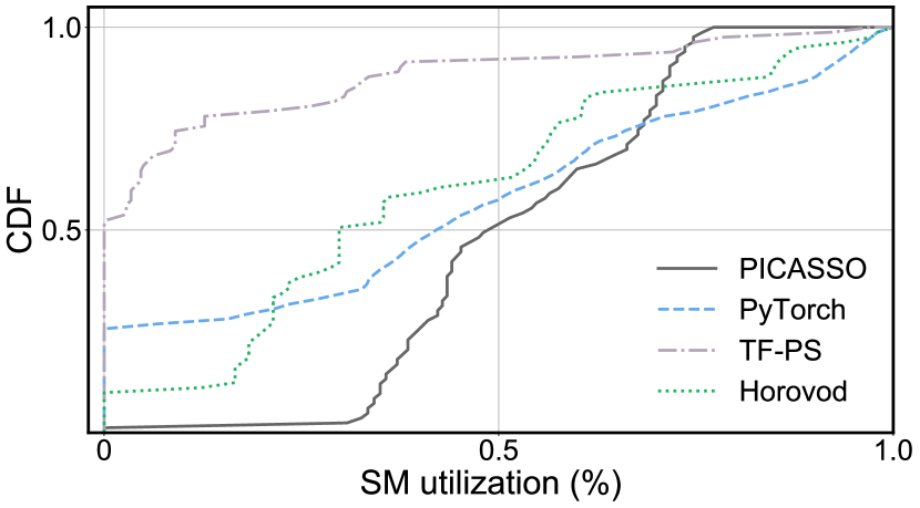
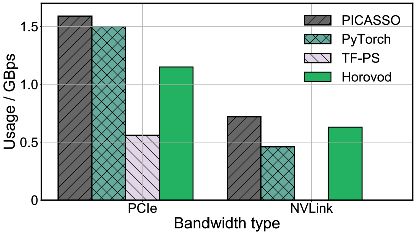
Hardware Utilization. We then investigate the runtime utilization of the underlying hardware when training the DLRM model, and we plot the GPU SM utilization and NVLink/PCIe bandwidth consumption in a 10-millisecond granularity in Fig. 12 and Fig. 12. Although the other frameworks optimize some phases of training (e.g., PyTorch and Horovod present intermittent high GPU SM utilization), they suffer from certain bottlenecks implied from the large CDF area of low GPU SM utilization. In contrast, PICASSO has barely any area of low GPU SM utilization, meaning that the bottlenecks on this testbed are effectively addressed by the software system optimization. In terms of bandwidth utilization, PICASSO is much better than the TF-PS baseline as leveraging the collective communication primitives and the hardware coherency via NVLink. When compared to Horovod and PyTorch, PICASSO still slightly improves bandwidth usage due to pipelines in interleaving. The improvement of hardware utilization indicates that though the generic frameworks have pushed the computation efficiency to a peak level, PICASSO still succeeds to unleash the potential of the underlying hardware resources.

Figure 13: Training performance of the three models by the three training systems in the in-house cluster.

Figure 14: Training performance by using 1 to 11 interleaving groups. The three models own 16, 19, 11 packed embedding respectively.

Figure 15: Training performance of scaling-out of PICASSO ranging from 1 to 128 workers in the in-house cluster.

IV-C Evaluation of System Design (RQ2)

TABLE IV: Ablation study on PICASSO

		IPS	PCIe (GBps)	Comm. (Gbps)	SM util. (%)
W&D	PICASSO	22,825	1.57	2.48	32
	w/o Packing	17,827	1.54	1.84	23
	w/o Interleaving	16,218	1.49	1.69	21
	w/o Caching	19,264	1.51	2.07	25
CAN	PICASSO	12,218	2.59	8.50	62
	w/o Packing	8,769	2.55	6.66	45
	w/o Interleaving	7,957	2.02	6.94	43
	w/o Caching	10,829	2.60	7.41	51
MMoE	PICASSO	2,546	2.31	6.61	98
	w/o Packing	2,270	2.27	6.10	96
	w/o Interleaving	1,319	1.87	3.80	64
	w/o Caching	2,401	2.28	6.44	98

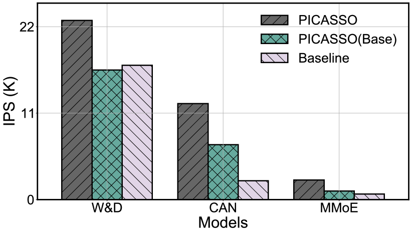
Industrial WDL workloads are usually much more complicated than the benchmarking workloads, regarding both model architecture and data distribution. We investigate the effectiveness of PICASSO in industry services by W&D, CAN, and MMoE models over industrial datasets. Meanwhile, we measure the fine-grained contribution of packing, interleaving and caching by training throughput. The evaluation is conducted over 16 nodes in the EFLOPS cluster if not specified explicitly. We use the commonly-used asynchronous PS strategy of Tensorflow at Alibaba as the baseline. We also implement PICASSO without software system optimization, denoted as “PICASSO(Base)”, which can be seen as a pure hybrid-parallel training strategy framework. Fig. 15 depicts the IPS, where we observe a 4$\times$ acceleration on CAN and MMoE. We then dive into the software system optimizations via an ablation study.

Ablation Study. We remove the software system optimization from PICASSO, in turn, to verify its effect on WDL tasks and collect metrics in Tab. IV.

By using the packing approach, the fragmentary operations on feature embedding are packed together, leading to an improvement on IPS by 30% and the correspondingly increased hardware usage of PCIe, network and GPU SMs. The interleaving approach utilizes pipelines to hide memory access and network latency by computation-intensive operations. Obviously, MMoE owns the most complicated computation workload among the three models and thus benefits most from this optimization. The interleaving approach significantly raises the performance of MMoE by 93%. This is consistent with the analysis that the two models suffer heavy computation load, and PICASSO helps diffuse the pulse-like GPU usage throughout the entire training process. W&D, not having sufficient computation, would benefit from the data-interleaving to mitigate the congestion on PCIe and network. Caching relies on leveraging the distribution of input data. Thus, we run 100 steps as a warm-up to collect the statistics and then set the Hot-storage size to 1GB on GPU memory to maintain the unique IDs’ hit ratio above 20% within each batch. HybridHash improves the performance by up to 13%, which attributes to a balanced utilization of PCIe and GPUs.

TABLE V: Number of operations in computational graph

Model	# of operations		# of packed embedding
	Baseline	PICASSO	Baseline	PICASSO
W&D	100,039	14,882 (14.9%)	204	16 (7.8%)
CAN	381,364	67,985 (17.8%)	364	19 (5.2%)
MMoE	300,524	75,217 (25.0%)	94	11 (11.7%)

Effectiveness of Packing. WDL models tend to own fragmentary operations for the multi-field embedding and feature interactions. We dump the computational graph of the three models through Baseline and PICASSO, and the number of operations and packed embedding are shown in Tab. V. The statistic implies that PICASSO dramatically reduces the fragmentary operations, even if the interleaving optimization supplements a certain amount of operations to pipeline the executions.

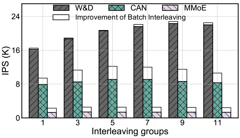
Interleaving Groups. The number of interleaving groups affects the efficiency of the embedding layer. Fig. 15 shows the throughput by varying the number of K-interleaving groups. Obviously, the communication-intensive workloads, i.e., W&D and CAN, can benefit from the increased interleaving as the combination of packed embedding uniformizes the usage of each hardware resource. We also see that the batch interleaving contributes differently to the models. The result reflects that utilizing more micro-batches would greatly improve the performance of the computation-intensive workload, i.e., CAN and MMoE, by meeting the saturation of GPU. It reveals that the interleaving strategies are effective for WDL workloads when there is sufficient input data and underutilized hardware.

TABLE VI: Hit ratio and IPS by varying the size of Hot-storage

Hot-Storage	W&D		CAN		MMoE
	Hit ratio	IPS	Hit ratio	IPS	Hit ratio	IPS
256MB	9%	-11%	20%	-19%	9%	-3%
512MB	18%	-5%	28%	-10%	16%	-1%
1GB	24%	+0%	37%	+0%	21%	+0%
2GB	28%	+1%	44%	+5%	24%	+0%
4GB	31%	-3%	45%	+2%	27%	-2%

Size of Hot-storage. In the industrial WDL workload, it is impossible to foresee the size of the embedding tables since the model should constantly deal with the newly-emerged categorical feature IDs. We set the size of Hot-storage to 1GB in the previous evaluations to ensure 20% hit ratio. Tab. VI depicts the cache hit ratio and improvement of IPS by varying the size of Hot-storage. Larger cache size carries more embedding, yet we find an apparent marginal effect of the hit ratio when the cache size reaches above 2GB. Although the large cache hits more ID queries, the occupation of GPU memory forces the training to compromise the batch size, leading to a slight reduction in the overall throughput. Hence, it is no need to pursue high cache hit ratio by setting an excessively large cache size in WDL workload.

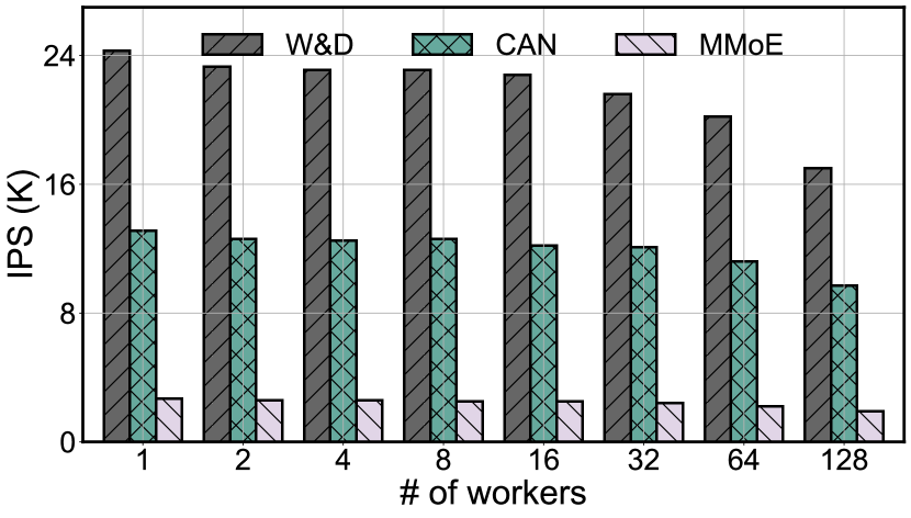
Scaling Out. We scale out the training clusters from one PICASSO-Executor to 128 PICASSO-Executors and illustrate the performance by IPS in Fig. 15. The correlation between IPS and the number of PICASSO-Executors shows that PICASSO achieves near-linear scalability on CAN and MMoE while attaining a sublinear throughput on W&D. This result implies that PICASSO can amortize the additional communication overhead from the increasing number of PICASSO-Executors and handle large-scale WDL training.

IV-D Applicability Experiment (RQ3)

TABLE VII: Training throughput of 12 AUC prediction models by PICASSO and in-house XDL.

Model	Batch size	GPU SM utilization	IPS
LR [35]	20K $\xrightarrow{}$ 36K (20K x 2)	9 $\xrightarrow{}$ 22 (+144%)	12.0K $\xrightarrow{}$ 25.9K (+115%)
W&D [2]	19K $\xrightarrow{}$ 36K (18K x 2)	21 $\xrightarrow{}$ 35 (+67%)	14.7K $\xrightarrow{}$ 22.2K (+50%)
TwoTowerDNN[36]	12K $\xrightarrow{}$ 36K (12K x 3)	35 $\xrightarrow{}$ 97 (+177%)	4.7K $\xrightarrow{}$ 12.1K (+160%)
DLRM [23]	10K $\xrightarrow{}$ 30K (10K x 3)	38 $\xrightarrow{}$ 98 (+158%)	3.8K $\xrightarrow{}$ 10.4K (+171%)
DCN [37]	14K $\xrightarrow{}$ 36K (12K x 3)	56 $\xrightarrow{}$ 92 (+64%)	9.0K $\xrightarrow{}$ 13.7K (+52%)
xDeepFM [38]	6K $\xrightarrow{}$ 20K (5K x 4)	45 $\xrightarrow{}$ 98 (+117%)	3.1K $\xrightarrow{}$ 5.9K (+89%)
ATBRG [39]	3K $\xrightarrow{}$ 6K (3K x 2)	13 $\xrightarrow{}$ 26 (+100%)	0.8K $\xrightarrow{}$ 1.4K (+82%)
DIN [4]	15K $\xrightarrow{}$ 45K (15K x 3)	34 $\xrightarrow{}$ 80 (+135%)	7.5K $\xrightarrow{}$ 16.0K (+113%)
DIEN [5]	15K $\xrightarrow{}$ 45K (15K x 3)	29 $\xrightarrow{}$ 75 (+159%)	7.3K $\xrightarrow{}$ 15.6K (+115%)
DSIN [40]	9K $\xrightarrow{}$ 27K (9K x 3)	40 $\xrightarrow{}$ 93 (+133%)	4.7K $\xrightarrow{}$ 9.8K (+111%)
CAN [8]	12K $\xrightarrow{}$ 48K (12K x 4)	17 $\xrightarrow{}$ 75 (+341%)	3.9K $\xrightarrow{}$ 12.1K (+210%)
STAR [25]	2K $\xrightarrow{}$ 8K (2K x 4)	32 $\xrightarrow{}$ 98 (+206%)	0.6K $\xrightarrow{}$ 2.0K (+215%)

Varying Feature Interactions. We further investigate the performance of PICASSO on more industrial-scale WDL models with various types of feature interaction modules. We select 12 AUC prediction models, and tune the hyperparameters to ensure the convergence of the models. The models are slightly modified to cope with the Product-2 dataset. To show the adaptability of PICASSO, we take the in-house optimized XDL as the baseline to train those models in synchronous PS training mode. The performance of the 12 models is listed in Table VII. Obviously, the proposed PICASSO significantly improves the GPU utilization compared to the in-house optimized XDL [41] framework. It indicates that with the software system optimization, PICASSO is able to be aware of the hardware bound, and unleash the hardware potential for various WDL model architectures.

TABLE VIII: Performance of CAN by varying number of feature fields on synthetic dataset

Feature field	1	2	3	4	5	6	7	8
PICASSO	12.20	6.14	4.13	3.13	2.50	2.09	1.82	1.61
AP	12.20	6.10	4.07	3.05	2.44	2.03	1.74	1.53
Increment	0.0%	+0.6%	+1.7%	+2.5%	+2.6%	+2.7%	+4.3%	+5.3%
XDL	2.40	1.18	0.75	0.56	0.42	0.36	0.31	0.25
AP	2.40	1.20	0.80	0.60	0.48	0.40	0.34	0.30
Increment	0.0%	-1.5%	-6.8%	-6.1%	-13.1%	-9.6%	-10.3%	-15.3%

Increasing Feature Fields. We present the performance of PICASSO by varying the number of feature fields. As currently we do not operate business that ingests thousands of feature fields, we make a synthetic dataset by duplicating the feature fields of Product-2. Therefore, the number of feature fields becomes an integral multiple of 364 in the data source. Correspondingly, we duplicate the feature interaction layers to process the synthetic dataset. The outputs of the feature interaction layers are concatenated together to feed to a mutual MLP. Tab. VIII depicts the IPS by PICASSO and the in-house optimized XDL, as well as the theoretical IPS by arithmetic progression (AP). Though the requirements of the underlying hardware resources increase by the number of feature fields, PICASSO performs slightly better than AP due to the packing of the fragmentary operations. In contrast, the PS baseline suffers from the massive operations by the large number of feature fields and the constituent feature interactions, thereby presenting significant IPS drop compared to AP.

Discussion. Evaluations show that PICASSO successfully unleashes the potential of hardware resources, where PICASSO uniformizes the hardware usage for high overall hardware utilization (RQ2) and provides diversified optimization for WDL models with different attributes (RQ3). Employing super-large batch size in training requires certain auxiliary approaches (e.g., global batch normalization [42], Lamb optimizer [43]), which can be applied in PICASSO through implementation in Tensorflow. Obviously, should we deploy customized hardware to enhance specific hardware resources, or if particular WDL tasks presented high tolerance for accuracy loss from the precision-lossy mechanisms, the performance of PICASSO will surely be further improved.

V Deployment in Production

TABLE IX: Performance of PICASSO at Alibaba Cloud

	Average task walltime (h)	GPU SM util. (%)	Bandwidth (Gbps)
XDL	8.6	15	1.412 (TCP)
PICASSO	1.4	75	6.851 (TCP+RDMA)

We implement PICASSO on top of Tensorflow. It has been deployed in our on-premises clusters since October 2020 to serve business of online and offline WDL tasks, including information retrieval, advertisement bidding, recommendation, and search ranking. Since we deployed PICASSO, training throughput has been greatly improved, and impressive performance has been achieved in a number of highly-promoted sales. In-house sophisticated scheduling and failover-recovery strategies are employed by PICASSO for robust training [44, 45], which are beyond this paper’s scope.

The arithmetic computation is still very heavy in training state-of-the-art WDL designs. Benefiting from popular CV and NLP training acceleration approaches, we have applied the latest solutions, such as GPU acceleration libraries (e.g., CUTLASS [46] and CuDNN [47]), operator-level graph replacement [48], compiler optimization [49], and quantitative communication[50] to PICASSO. We also implement topology-aware communication[51] to avoid IO tasks on GPU devices from the same node competing for limited NIC resources. These accelerations are orthogonal to the optimization of PICASSO. We provide users with a flexible interface to invoke these methods when tuning their design. Other emerging technologies can be integrated into PICASSO via the Tensorflow ecosystem.

We instrument a production training cluster of one Tesla-V100 per worker, which runs hundreds of daily WDL workloads. These workloads present remarkably different training intensities by various input features, embedding dimensions, feature interaction modules, and shapes of MLP. We record job statistics of the succeeded training tasks from Jun. 1st, 2021, to Nov. 15th, 2021. To make a comparison, we prepare previously deployed XDL [41] in another production cluster with comparable types of workloads. The results in Tab. IX show that PICASSO brings around 6$\times$ performance acceleration on average and contributes to improving the utilization of underlying hardware. The throughput acceleration reduces the delay of daily continuous delivery by 7 hours on average. We further probe into several representative models (with entirely different model architecture and data distribution) from the monitored cluster and present the required walltime over 128 Tesla-V100s to train petabyte-scale data accumulated by one year as shown in Tab. X. The statistics reveal that PICASSO reduces model training of 100-billion-scale parameters from one month to 2 days. Moreover, regarding a WDL model with 1-trillion-scale parameters (one of the currently largest models satisfying real-time inference throughput demand in our business), the training completes within nine days, while the baseline framework is estimated to occupy the resources for more than three months. This training acceleration is critical in the latest ML/DL trends of providing high WDL business value.

VI Related Work

We summarize the trending research approaches with respect to training WDL jobs into three categories as follows:

Hardware Customization. For a specific WDL workload with a high business value, it is profitable to customize the hardware itself to achieve a cutting-edge performance and throughput. AIBox/PaddleBox [52, 53] leverages non-volatile memory to drastically reduce the training scale from an MPI cluster with hundreds of CPUs to a single machine with 8 GPUs. HugeCTR/Merlin is a customized framework running on NVIDIA’s DGX-1/DGX-2 supernodes equipped with high-end interconnects named NV-Switch. Zion [12] and RecSpeed [54] customize their node specification for DLRM [23] and its variants by adding more NICs and RoCEs to alleviate the I/O bottleneck. Nevertheless, hardware customization is still expensive and a waste of resources when facing rapid shifts in WDL designs. Further, training systems upon customized hardware are difficult to scale out on cloud elastically.

TABLE X: Walltime (GPU-core hour) to train data accumulated by one year (“P” indicates the predicted walltime)

Model scale	$\sim$ 1B	$\sim$ 10B	$\sim$ 100B	$\sim$ 1T
XDL	2,072	11,013	88,129 (P)	323,480 (P)
PICASSO	747	2,285	6,091	27,256

Subsystem Optimization. Subsystem optimization diagnoses specific bottlenecks and improves the performance of certain workloads. For example, the communication protocol in BytePS [55] accelerates the data exchange in PS strategy. Kraken [56] develops memory-efficient table structure to hold parameters of embedding layers. ScaleFreeCTR [57] utilizes GPU to accelerate the embedding lookup of parameters stored in DRAM. Het [58] introduces staleness to embedding update which is suitable for the WDL designs with small-size local embedding tables. These optimizations are likely to miss opportunities of improving overall performance systematically owing to the unawareness of either sparse manipulation or intensive computation of WDLs, while precision-lossy operations like staleness would do harm to the E-commerce WDL models.

Generic DNN Training Optimization. There are already a variety of proposed training frameworks targeting dense models from domains such as CV and NLP. These frameworks provide meticulous strategies for splitting and pipelining workloads during training. Megatron [59] speeds up the transformer module in NLP workloads. GPipe [60] implements pipeline over mini batches, and Pipedream [61] further fills the bubble between forward and backward pass by weight stashing. GShard [62] relies on a compilation approach to shard parameters and activations. Unfortunately, WDL models are usually sensitive to numeric precision and gradient staleness [63, 64, 65], and WDL workload has much more operators on dynamic shape of data than CV and NLP models. Hence, these generic DNN training optimizations may not apply to WDL workload at an industrial scale.

VII Conclusion

In this paper, we introduce PICASSO, a deep learning training system upon Tensorflow, to accelerate the training of WDL models on commodity hardware with the awareness of model architecture and data distribution. With the investigation of representative workloads at Alibaba Cloud, we design an advantageous training framework and provide workload-aware software optimization: 1) packing the embedding tables and the subsequent operations to reduce the fragmentary operations that are not friendly to GPU-centric training; 2) interleaving the embedding layer and the feature interaction to diffuse the pulse-like usage throughout the entire training process; 3) caching the frequently-visited categorical IDs to expedite the repeated embedding queries. Product deployment at Alibaba Cloud demonstrates that a 1-trillion parameter WDL model through one-year petabyte-scale data can be efficiently trained in 27,256 GPU core hours, significantly reducing the training cost by a factor of 12. PICASSO helps decrease the delay of daily continuous delivery by 7 hours, which is crucially important for state-of-the-art recommender systems.

References

- [1] J. B. Schafer, D. Frankowski, J. Herlocker, and S. Sen, “Collaborative filtering recommender systems,” in The adaptive web. Springer, 2007, pp. 291–324.
- [2] H.-T. Cheng, L. Koc, J. Harmsen, T. Shaked, T. Chandra, H. Aradhye, G. Anderson, G. Corrado, W. Chai, M. Ispir et al., “Wide & deep learning for recommender systems,” in Proceedings of the 1st workshop on deep learning for recommender systems, 2016, pp. 7–10.
- [3] H. Guo, R. TANG, Y. Ye, Z. Li, and X. He, “Deepfm: A factorization-machine based neural network for ctr prediction,” in Proceedings of the Twenty-Sixth International Joint Conference on Artificial Intelligence, IJCAI-17, 2017, pp. 1725–1731.
- [4] G. Zhou, X. Zhu, C. Song, Y. Fan, H. Zhu, X. Ma, Y. Yan, J. Jin, H. Li, and K. Gai, “Deep interest network for click-through rate prediction,” in Proceedings of the 24th ACM SIGKDD International Conference on Knowledge Discovery & Data Mining, 2018, pp. 1059–1068.
- [5] G. Zhou, N. Mou, Y. Fan, Q. Pi, W. Bian, C. Zhou, X. Zhu, and K. Gai, “Deep interest evolution network for click-through rate prediction,” in Proceedings of the AAAI conference on artificial intelligence, vol. 33, 2019, pp. 5941–5948.
- [6] M. Naumov, D. Mudigere, H.-J. M. Shi, J. Huang, N. Sundaraman, J. Park, X. Wang, U. Gupta, C.-J. Wu, A. G. Azzolini et al., “Deep learning recommendation model for personalization and recommendation systems,” arXiv preprint arXiv:1906.00091, 2019.
- [7] P. Qi, X. Zhu, G. Zhou, Y. Zhang, Z. Wang, L. Ren, Y. Fan, and K. Gai, “Search-based user interest modeling with lifelong sequential behavior data for click-through rate prediction,” in Proceedings of the 29th ACM International Conference on Information & Knowledge Management, 2020.
- [8] G. Zhou, W. Bian, K. Wu, L. Ren, Q. Pi, Y. Zhang, C. Xiao, X.-R. Sheng, N. Mou, X. Luo et al., “Can: Revisiting feature co-action for click-through rate prediction,” arXiv preprint arXiv:2011.05625, 2020.
- [9] L. Chen, “Continuous delivery: Huge benefits, but challenges too,” IEEE software, vol. 32, no. 2, pp. 50–54, 2015.
- [10] M. Li, D. G. Andersen, J. W. Park, A. J. Smola, A. Ahmed, V. Josifovski, J. Long, E. J. Shekita, and B.-Y. Su, “Scaling distributed machine learning with the parameter server,” in 11th USENIX Symposium on Operating Systems Design and Implementation (OSDI 14), 2014, pp. 583–598.
- [11] W. Zhao, D. Xie, R. Jia, Y. Qian, R. Ding, M. Sun, and P. Li, “Distributed hierarchical gpu parameter server for massive scale deep learning ads systems,” in Proceedings of Machine Learning and Systems, I. Dhillon, D. Papailiopoulos, and V. Sze, Eds., vol. 2, 2020, pp. 412–428.
- [12] M. Smelyanskiy, “Zion: Facebook next-generation large memory training platform,” in 2019 IEEE Hot Chips 31 Symposium (HCS). IEEE Computer Society, 2019, pp. 1–22.
- [13] J. Chung, C. Gulcehre, K. Cho, and Y. Bengio, “Empirical evaluation of gated recurrent neural networks on sequence modeling,” NIPS 2014 Workshop on Deep Learning, 2014.
- [14] A. Vaswani, N. Shazeer, N. Parmar, J. Uszkoreit, L. Jones, A. N. Gomez, Ł. Kaiser, and I. Polosukhin, “Attention is all you need,” in Advances in neural information processing systems, 2017, pp. 5998–6008.
- [15] S. Ioffe and C. Szegedy, “Batch normalization: Accelerating deep network training by reducing internal covariate shift,” in Proceedings of the 32nd International Conference on International Conference on Machine Learning - Volume 37, 2015, p. 448–456.
- [16] K. He, X. Zhang, S. Ren, and J. Sun, “Deep residual learning for image recognition,” in Proceedings of the IEEE conference on computer vision and pattern recognition, 2016, pp. 770–778.
- [17] D. Alistarh, D. Grubic, J. Li, R. Tomioka, and M. Vojnovic, “Qsgd: Communication-efficient sgd via gradient quantization and encoding,” Advances in Neural Information Processing Systems, vol. 30, pp. 1709–1720, 2017.
- [18] H.-T. Cheng, Z. Haque, L. Hong, M. Ispir, C. Mewald, I. Polosukhin, G. Roumpos, D. Sculley, J. Smith, D. Soergel et al., “Tensorflow estimators: Managing simplicity vs. flexibility in high-level machine learning frameworks,” in Proceedings of the 23rd ACM SIGKDD International Conference on Knowledge Discovery and Data Mining, 2017, pp. 1763–1771.
- [19] S. Li, Y. Zhao, R. Varma, O. Salpekar, P. Noordhuis, T. Li, A. Paszke, J. Smith, B. Vaughan, P. Damania, and S. Chintala, “Pytorch distributed: Experiences on accelerating data parallel training,” Proc. VLDB Endow., vol. 13, no. 12, p. 3005–3018, 2020.
- [20] J. Dean, G. S. Corrado, R. Monga, K. Chen, M. Devin, Q. V. Le, M. Z. Mao, M. Ranzato, A. Senior, P. Tucker et al., “Large scale distributed deep networks,” 2012.
- [21] S. Kim, G.-I. Yu, H. Park, S. Cho, E. Jeong, H. Ha, S. Lee, J. S. Jeong, and B.-G. Chun, “Parallax: Sparsity-aware data parallel training of deep neural networks,” in Proceedings of the Fourteenth EuroSys Conference 2019, 2019, pp. 1–15.
- [22] J. Dong, Z. Cao, T. Zhang, J. Ye, S. Wang, F. Feng, L. Zhao, X. Liu, L. Song, L. Peng et al., “Eflops: Algorithm and system co-design for a high performance distributed training platform,” in 2020 IEEE International Symposium on High Performance Computer Architecture (HPCA). IEEE, 2020, pp. 610–622.
- [23] D. Mudigere, Y. Hao, J. Huang, A. Tulloch, S. Sridharan, X. Liu, M. Ozdal, J. Nie, J. Park, L. Luo et al., “software hardware co-design for fast and scalable training of deep learning recommender system,” arXiv preprint arXiv:2104.05158, 2021.
- [24] Z. Zhao, L. Hong, L. Wei, J. Chen, A. Nath, S. Andrews, A. Kumthekar, M. Sathiamoorthy, X. Yi, and E. Chi, “Recommending what video to watch next: a multitask ranking system,” in Proceedings of the 13th ACM Conference on Recommender Systems, 2019, pp. 43–51.
- [25] X.-R. Sheng, L. Zhao, G. Zhou, X. Ding, Q. Luo, S. Yang, J. Lv, C. Zhang, and X. Zhu, “One model to serve all: Star topology adaptive recommender for multi-domain ctr prediction,” in Proceedings of the 29th ACM International Conference on Information & Knowledge Management, 2021.
- [26] A. W. Senior, R. Evans, J. Jumper, J. Kirkpatrick, L. Sifre, T. Green, C. Qin, A. Žídek, A. W. Nelson, A. Bridgland et al., “Improved protein structure prediction using potentials from deep learning,” Nature, vol. 577, no. 7792, pp. 706–710, 2020.
- [27] Y. Wei, X. Wang, L. Nie, X. He, R. Hong, and T.-S. Chua, “Mmgcn: Multi-modal graph convolution network for personalized recommendation of micro-video,” in Proceedings of the 27th ACM International Conference on Multimedia, 2019, pp. 1437–1445.
- [28] D. A. Patterson and J. L. Hennessy, Computer Organization and Design ARM Edition: The Hardware Software Interface. Morgan kaufmann, 2016.
- [29] C. AILab, “Download criteo 1tb click logs dataset,” https://ailab.criteo.com/download-criteo-1tb-click-logs-dataset/.
- [30] M. Association, “Machine learning innovation to benefit everyone,” https://mlperf.org/.
- [31] Google, “Tensorflow release 1.15.0,” https://github.com/tensorflow/tensorflow/releases/tag/v1.15.0.
- [32] Facebook, “Pytorch,” https://github.com/pytorch/pytorch.
- [33] A. Sergeev and M. Del Balso, “Horovod: fast and easy distributed deep learning in tensorflow,” arXiv preprint arXiv:1802.05799, 2018.
- [34] N. Corporation, “Manage and monitor gpus in cluster environments,” https://developer.nvidia.com/dcgm.
- [35] K. Gai, X. Zhu, H. Li, K. Liu, and Z. Wang, “Learning piece-wise linear models from large scale data for ad click prediction,” arXiv preprint arXiv:1704.05194, 2017.
- [36] M. Fan, J. Guo, S. Zhu, S. Miao, M. Sun, and P. Li, “Mobius: towards the next generation of query-ad matching in baidu’s sponsored search,” in Proceedings of the 25th ACM SIGKDD International Conference on Knowledge Discovery & Data Mining, 2019, pp. 2509–2517.
- [37] R. Wang, B. Fu, G. Fu, and M. Wang, “Deep & cross network for ad click predictions,” in Proceedings of the ADKDD’17, 2017, pp. 1–7.
- [38] J. Lian, X. Zhou, F. Zhang, Z. Chen, X. Xie, and G. Sun, “xdeepfm: Combining explicit and implicit feature interactions for recommender systems,” in Proceedings of the 24th ACM SIGKDD International Conference on Knowledge Discovery & Data Mining, 2018, pp. 1754–1763.
- [39] Y. Feng, B. Hu, F. Lv, Q. Liu, Z. Zhang, and W. Ou, “Atbrg: Adaptive target-behavior relational graph network for effective recommendation,” in Proceedings of the 43rd International ACM SIGIR Conference on Research and Development in Information Retrieval, 2020, pp. 2231–2240.
- [40] Y. Feng, F. Lv, W. Shen, M. Wang, F. Sun, Y. Zhu, and K. Yang, “Deep session interest network for click-through rate prediction,” in Proceedings of the Twenty-Eighth International Joint Conference on Artificial Intelligence, IJCAI-19. International Joint Conferences on Artificial Intelligence Organization, 2019, pp. 2301–2307.
- [41] B. Jiang, C. Deng, H. Yi, Z. Hu, G. Zhou, Y. Zheng, S. Huang, X. Guo, D. Wang, Y. Song et al., “Xdl: an industrial deep learning framework for high-dimensional sparse data,” in Proceedings of the 1st International Workshop on Deep Learning Practice for High-Dimensional Sparse Data, 2019, pp. 1–9.
- [42] T. Chen, S. Kornblith, M. Norouzi, and G. Hinton, “A simple framework for contrastive learning of visual representations,” in International conference on machine learning. PMLR, 2020, pp. 1597–1607.
- [43] Y. You, J. Li, S. Reddi, J. Hseu, S. Kumar, S. Bhojanapalli, X. Song, J. Demmel, K. Keutzer, and C.-J. Hsieh, “Large batch optimization for deep learning: Training bert in 76 minutes,” in ICLR, 2019.
- [44] Y. Huang, Y. Shi, Z. Zhong, Y. Feng, J. Cheng, J. Li, H. Fan, C. Li, T. Guan, and J. Zhou, “Yugong: Geo-distributed data and job placement at scale,” Proceedings of the VLDB Endowment, vol. 12, no. 12, pp. 2155–2169, 2019.
- [45] Y. Feng, Z. Liu, Y. Zhao, T. Jin, Y. Wu, Y. Zhang, J. Cheng, C. Li, and T. Guan, “Scaling large production clusters with partitioned synchronization,” in 2021 USENIX Annual Technical Conference (USENIXATC 21), 2021, pp. 81–97.
- [46] N. Corporation, “Cutlass: Fast linear algebra in cuda c++,” https://developer.nvidia.com/blog/cutlass-linear-algebra-cuda/, may 21, 2018.
- [47] ——, “Nvidia cuda®deep neural network library,” https://developer.nvidia.com/CUDNN/.
- [48] T. Chen, T. Moreau, Z. Jiang, L. Zheng, E. Yan, H. Shen, M. Cowan, L. Wang, Y. Hu, L. Ceze et al., “TVM: An automated end-to-end optimizing compiler for deep learning,” in 13th USENIX Symposium on Operating Systems Design and Implementation (OSDI 18), 2018, pp. 578–594.
- [49] J. Dean, “Machine learning for systems and systems for machine learning,” in Presentation at 2017 Conference on Neural Information Processing Systems, 2017.
- [50] P. Jiang and G. Agrawal, “A linear speedup analysis of distributed deep learning with sparse and quantized communication,” in Proceedings of the 32nd International Conference on Neural Information Processing Systems, 2018, pp. 2530–2541.
- [51] J. Dong, S. Wang, F. Feng, Z. Cao, H. Pan, L. Tang, P. Li, H. Li, Q. Ran, Y. Guo et al., “Accl: Architecting highly scalable distributed training systems with highly efficient collective communication library,” IEEE Micro, vol. 41, no. 5, pp. 85–92, 2021.
- [52] W. Zhao, J. Zhang, D. Xie, Y. Qian, R. Jia, and P. Li, “Aibox: Ctr prediction model training on a single node,” in Proceedings of the 28th ACM International Conference on Information and Knowledge Management, 2019, pp. 319–328.
- [53] W. Zhao, D. Xie, R. Jia, Y. Qian, R. Ding, M. Sun, and P. Li, “Distributed hierarchical gpu parameter server for massive scale deep learning ads systems,” in Proceedings of the 3rd MLSys Conference, 2020.
- [54] S. Krishna and R. Krishna, “Accelerating recommender systems via hardware” scale-in”,” arXiv preprint arXiv:2009.05230, 2020.
- [55] Y. Peng, Y. Zhu, Y. Chen, Y. Bao, B. Yi, C. Lan, C. Wu, and C. Guo, “A generic communication scheduler for distributed dnn training acceleration,” in Proceedings of the 27th ACM Symposium on Operating Systems Principles, 2019, pp. 16–29.
- [56] M. Xie, K. Ren, Y. Lu, G. Yang, Q. Xu, B. Wu, J. Lin, H. Ao, W. Xu, and J. Shu, “Kraken: memory-efficient continual learning for large-scale real-time recommendations,” in 2020 SC20: International Conference for High Performance Computing, Networking, Storage and Analysis (SC). IEEE Computer Society, 2020, pp. 278–294.
- [57] H. Guo, W. Guo, Y. Gao, R. Tang, X. He, and W. Liu, “Scalefreectr: Mixcache-based distributed training system for ctr models with huge embedding table,” in SIGIR, 2021.
- [58] X. Miao, H. Zhang, Y. Shi, X. Nie, Z. Yang, Y. Tao, and B. Cui, “Het: Scaling out huge embedding model training via cache-enabled distributed framework,” Proc. VLDB Endow., pp. 1–9, 2021.
- [59] M. Shoeybi, M. Patwary, R. Puri, P. LeGresley, J. Casper, and B. Catanzaro, “Megatron-lm: Training multi-billion parameter language models using model parallelism,” arXiv preprint arXiv:1909.08053, 2019.
- [60] Y. Huang, Y. Cheng, A. Bapna, O. Firat, M. X. Chen, D. Chen, H. Lee, J. Ngiam, Q. V. Le, Y. Wu et al., “Gpipe: Efficient training of giant neural networks using pipeline parallelism,” in NeurIPS, 2019.
- [61] D. Narayanan, A. Harlap, A. Phanishayee, V. Seshadri, N. R. Devanur, G. R. Ganger, P. B. Gibbons, and M. Zaharia, “Pipedream: generalized pipeline parallelism for dnn training,” in Proceedings of the 27th ACM Symposium on Operating Systems Principles, 2019, pp. 1–15.
- [62] D. Lepikhin, H. Lee, Y. Xu, D. Chen, O. Firat, Y. Huang, M. Krikun, N. Shazeer, and Z. Chen, “Gshard: Scaling giant models with conditional computation and automatic sharding,” in ICLR, 2021.
- [63] A. Xu, Z. Huo, and H. Huang, “Step-ahead error feedback for distributed training with compressed gradient,” in Proceedings of the AAAI Conference on Artificial Intelligence, vol. 35, no. 12, 2021, pp. 10 478–10 486.
- [64] H. Zhuang, Z. Weng, F. Luo, T. Kar-Ann, H. Li, and Z. Lin, “Accumulated decoupled learning with gradient staleness mitigation for convolutional neural networks,” in International Conference on Machine Learning. PMLR, 2021, pp. 12 935–12 944.
- [65] Z. Cai and N. Vasconcelos, “Rethinking differentiable search for mixed-precision neural networks,” in Proceedings of the IEEE/CVF Conference on Computer Vision and Pattern Recognition, 2020, pp. 2349–2358.