SplitNets: Designing Neural Architectures
for Efficient Distributed Computing on Head-Mounted Systems

Abstract

We design deep neural networks (DNNs) and corresponding networks’ splittings to distribute DNNs’ workload to camera sensors and a centralized aggregator on head mounted devices to meet system performance targets in inference accuracy and latency under the given hardware resource constraints. To achieve an optimal balance among computation, communication, and performance, a split-aware neural architecture search framework, SplitNets, is introduced to conduct model designing, splitting, and communication reduction simultaneously. We further extend the framework to multi-view systems for learning to fuse inputs from multiple camera sensors with optimal performance and systemic efficiency. We validate SplitNets for single-view system on ImageNet as well as multi-view system on 3D classification, and show that the SplitNets framework achieves state-of-the-art (SOTA) performance and system latency compared with existing approaches.

1 Introduction

Figure 1: AR/VR device with multiple intelligent AI cameras.

Figure 2: Distributed inference with sensors and an aggregator. In this work, we focus on single/multi-view classification tasks.

Advantages	$\bm{\downarrow}$ Comm. Cost	$\bm{\downarrow}$ Peak Sensor Mem.	$\bm{\uparrow}$ Parallelism	$\bm{\uparrow}$ Hardware Utilization	Privacy Preserving
All on sensors	✓	✗	✓	✗	✓
All on aggregator	✗	✓	✗	✗	✗
Distributed computing	✓	✓	✓	✓	✓

Table 1: Comparison of different DNN computing offload paradigms.

Components	System factors to be considered
[regular] Sensor	$\square$ $\checkmark$ Computation capability    $\square$ $\checkmark$ Peak memory constraint    $\square$ $\checkmark$ Number of sensors (i.e., parallelism)
Comm.	$\square$ $\checkmark$ Communication bandwidth
Aggregator	$\square$ $\checkmark$ Computation capability
Whole system	$\square$ $\checkmark$ Task performance (e.g., accuracy)    $\square$ $\checkmark$ Overall latency = on-sen. latency         + comm. latency + on-agg. latency

Table 2: Factors need to be balanced when distributing DNN computation. The listed factors are interwoven with each other and have to be considered holistically.

Virtual Reality (VR) and Augmented Reality (AR) are becoming increasingly prevailing as one of the next-generation computing platforms [3]. Head mounted devices (HMD) for AR/VR feature multiple cameras to support various computer vision (CV) / machine learning (ML) powered human-computer interaction functions, such as object classification [40, 61], hand-tracking [19] and SLAM [38].

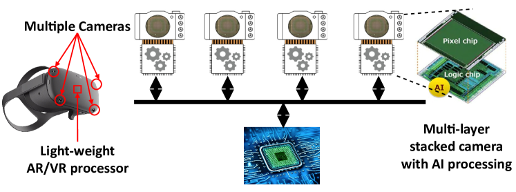
Due to the recent advances of camera technologies, tiny multi-layer stacked cameras with AI computing capability arise [32, 33], as depicted in Figure 1. Because of the small form factor, these intelligent cameras have highly constrained resources compared with general purpose mobile or data center grade AI processors. However, each camera is still capable of performing pre-processing directly after image acquisition, significantly reducing expensive raw image data movement. In a modern HMD system, the distributed intelligent stacked image sensors and a central AR/VR processor (aggregator) form the hardware backbone to realize complex CV/ML functions on device [3, 14, 13].

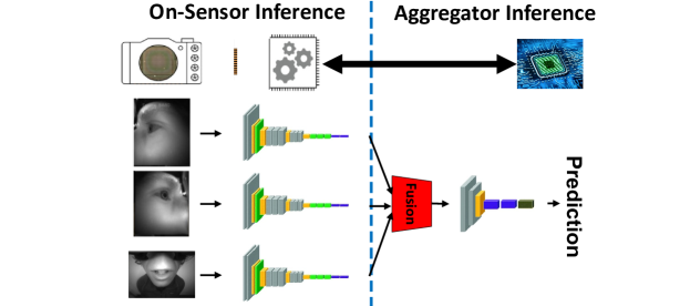
Within such systems, it’s natural to split the machine learning workload for an application between the sensors and the centralized computer (aggregator). As is shown in Figure 2, for an application that requires multiple layers of convolutional neural networks and fusion of multiple input sources, the early layers can be distributed to the on-sensor processing. The feature fusion and rest of processing are on the aggregator. This way, overall system latency can be improved by leveraging direct parallel processing on sensors and reduced sensor-aggregator communication.

The success of distributed computing for DNNs between sensors and aggregator heavily relies on the network architecture to satisfy the application and hardware system constraints such as memory, communication bandwidth, latency target and etc.. Prior work [27, 28, 10, 39] searches network partitions (i.e., the splitting points) for existing models in either exhaustive or heuristic manners. Some work [11, 46, 36, 4, 45] manually injects a bottleneck module into the model to reduce communication. However, these methods sometimes obtain naive splitting results (i.e., splitting after the last layer) [28] and lead to performance degradation [35].

The challenge of splitting DNNs comes from the complicated mutual-impact of many model and hardware factors. For example, existing (hand-crafted and searched) model architectures are designed without considering distributed computing over multiple computing modelities, and thus not suitable for splitting in the first place. In addition, the position of the splitting point as well as the inserted compression module will simultaneously impact model performance, computation offload, communication, and hardware utilization in different directions [37]. Heuristic and rule-based methods are limited in this context.

In this work, we adapt the neural architecture search (NAS) approach to automatically search split-aware model architectures targeting the distributed computing systems on AR/VR glasses. We propose the SplitNets framework that jointly optimizes the task performance and system efficiency subject to resource constraints of the mobile AR/VR system featuring smart sensors. We specifically answer the following two questions:

1. Can we jointly search for optimal network architectures and their network splitting solution between sensors and the aggregator while satisfying resource constraints imposed by the underlining hardware?

2. Can we learn an optimal network architecture to compress and fuse features from multiple sensors to the aggregator and achieve SOTA performance and efficiency compared with conventional centralized models?

We design SplitNets, a split-aware NAS framework, for efficient and flexible searching of the splitting module in the network in the distributed computing context where the splitting module is able to split the network, compress features along the channel dimension for communication saving as well as view fusion for multi-view tasks.

We introduce a series of techniques for module initialization and sampling to stabilize the training with information bottlenecks and mitigate introduced accuracy degradation. We further extend SplitNets to support searching of splitting modules with view fusion for multi-view tasks. To our best knowledge, it is the first framework supporting the position searching of information compression / fusion in a multi-input neural network. Overall, our contributions are summarized as follows:

• We propose SplitNets, a split-aware NAS framework, for efficient and flexible position searching of splitting modules for single / multi-view task.

• We introduce splitting modules for single- and multi- view tasks which can achieve model splitting, feature compression, as well as view fusion simultaneously. To search the optimal position of the splitting module, we propose to use separate supernets for sensors and the aggregator respectively, and stitch them together to form the split-aware model of interest, using the shared splitting module as the joint point. In addition, we combine the compression- / recovery- / fusion- based splitting module design with custom weights initialization, and a novel candidate networks sampling strategy to mitigate the accuracy drop due to model partition.

• We evaluate SplitNets with single-view classification and multi-view 3D classification. Empirical observations validate the importance of joint model and splitting position search to improve both task and system performance. Our results show that optimized network architectures and model partitions discovered by SplitNets significantly outperform existing solutions and fit the distributed computing system well on AR/VR glasses.

2 Background and Related Work

We consider a system that consists of three kinds of components, $V$ sensors, one aggregator, and communication interfaces between any of sensors and the aggregator. For simplicity, we assume that sensors are homogeneous.

A DNN is a composition of layers / computation which can be distributed to sensors and aggregator. Compared with on-sensor computing (All-on-sensor) and conventional mobile computing (All-on-aggregator), distributed computing has the flexibility to achieve a better balance between computation and communication, and enable high utilization of hardware, as summarized in Table 1.

A challenge is to determine a splitting point in the DNN. The on-sensor (on-sen.) part $f_{\texttt{sen}}$, which is composed of all layers of the DNN before the splitting point, is executed on sensors’ processors. The feature ${\mathbf{z}}$ generated by each sensor will be uploaded to the aggregator. The on-aggregator (on-agg.) part $f_{\texttt{agg}}$, which consists of all remaining layers of the DNN after the splitting point, receives ${\mathbf{z}}$ and finishes its computation on the computationally more capable aggregator processor.

The problem of finding the optimal splitting point can be summarized as follows,

$$\begin{split}\min_{f_{\texttt{sen}},f_{\texttt{agg}}}T_{\texttt{sen}}(f_{\texttt{sen}},{\mathbf{x}})+T_{\texttt{comm}}({\mathbf{z}})&+T_{\texttt{agg}}(f_{\texttt{agg}},{\mathbf{z}})\\ \text{where}\quad{\mathbf{z}}=f_{\texttt{sen}}({\mathbf{x}})\\ \text{s.t.}\quad\mathcal{L}(f_{\texttt{agg}}\circ f_{\texttt{sen}};\mathcal{D}^{\texttt{val}})&\leq\mathrm{Loss\ \ target}\\ \operatorname{PeakMem}(f_{\texttt{sen}},{\mathbf{x}})&\leq\operatorname{Mem}_{\texttt{sen}},\\ \end{split}$$ (1)

where $T(\cdot,\leavevmode\nobreak\ \cdot)$ is latency measurement function and $\mathcal{L}$ is the loss function, e.g., cross entropy. $\operatorname{PeakMem}(\cdot,\leavevmode\nobreak\ \cdot)$ measures the peak memory consumption of the on-sensor part, and $\operatorname{Mem}_{\texttt{sen}}$ is the memory size of a sensor processor.

To find the optimal splitting point, one has to take several factors into consideration simultaneously as summarized in Table 2. Existing solutions only consider a fraction of these factors via heuristic or exhaustive approaches [27, 28, 10, 39]. DNNs typically have tens or even hundreds of layers. Therefore, exhaustive searching with retraining is costly. Some literature proposes injecting a hand-crafted compression module to reduce the feature communication [11, 46, 36, 4, 45]. However, manually designing and inserting the compression module not only lead to high engineering effort and training cost, but also result in sub-optimal system performance and accuracy degradation.

In addition, previous methods all consider to split existing models like VGG [47] and ResNet [22]. However, those models may not be suitable for splitting. For example, Kang et al. [28] profiles seven models and finds that their best splitting points typically fall in the first or the last layers. Furthermore, injecting compression module to existing models usually leads to significant accuracy drop [36].

Other work proposes dedicated lossy (or lossless) compression techniques to reduce intermediate activation and save communication, including compressive sensing [59], pruning [26] and quantization [29, 6, 8]. SplitNets are orthogonal to, and can benefit from these prior approaches.

3 Split-Aware NAS

We adapt NAS to solve the constrained optimization in Equation 1. The goal is to minimize the systemic latency $T_{\texttt{sen}}+T_{\texttt{comm}}+T_{\texttt{agg}}$, and improve task performance while satisfying the hardware constraints.

We search the whole model $f_{\texttt{sen}}\circ f_{\texttt{agg}}$ and the position of splitting point, denoted as Split-Aware- NAS (or SA-NAS). This way, all layers before (or after) the splitting point will compose $f_{\texttt{sen}}$ or $f_{\texttt{agg}}$, respectively. In addition, we also consider a splitting module which is inserted at the position of splitting point. The feature compression in the splitting module can reduce communication cost by reducing the channel size $c$ of feature tensor ${\mathbf{z}}\in\mathbb{R}^{c\times s\times s}$, but could affect training stability and result in loss of task performance. We propose several approaches to mitigate the issue. The splitting module evolves along with $f_{\texttt{sen}}$ and $f_{\texttt{agg}}$ during SA-NAS as elaborated in Section 3.1.3. Eventually, the searched network must have exactly one splitting module.

Preliminary: Two-stage NAS Previous NAS approaches that leverage evolutionary search [43, 42, 50, 58] or reinforcement learning [52, 62, 63, 64] require excessive training due to the large number of models to be trained in a single experiment. Recent advancement of NAS decouples the model training and architecture search into two separate stages [60, 18, 7, 5, 55] that significantly reduces the training cost. In a two-stage NAS framework, the model training stage optimizes a supernet and its all sub-networks with weight-sharing. In the subsequent architecture optimization stage, sub-networks are searched based on system constraints to yield the best task and system performance trade-off. Due to the above advantages, we construct our SA-NAS based on two-stage NAS framework.

3.1 Building and Training Supernet (Stage 1)

Backbone of Supernet We build the supernet’s search space following FBNet-V3 [9] which uses the MobileNetv2 block (denoted as MB, a.k.a., inverted residual block) [44] as meta architecture. Check Appendix C for more details. We augment the supernet with SA-NAS specific search space (Figure 3) for our experiments as discussed in the following two sections.

3.1.1 SA-NAS for Single-View SplitNets

Now we elaborate how to search SplitNets for a single-view task (e.g., ImageNet classification), on searching the position of a splitting module, as shown in Figure 3.

Figure 3: Architecture sampling space in training SA-NAS. Both on-sen. and on-agg. networks consist of multiple phases with each containing a split module, flexible blocks before stride, a stride-2 block, and flexible blocks after stride. The splitting module can be a reduce operator (on-sen., green) or a recover / fuse operator (on-agg., purple). SA-NAS also includes standard NAS search space (blue) such as input resolution, channel widths, and etc.

Figure 4: SA-NAS for single-view SplitNets. At each training step, several sub-networks are sampled from the search space. A sub-network is specified by a set of choices including on-sen. blocks, splitting position, on-agg. blocks and blocks’ configurations. For single-view, weight-sharing between on-sen. and on-agg. blocks are enabled since they are learning similar features.

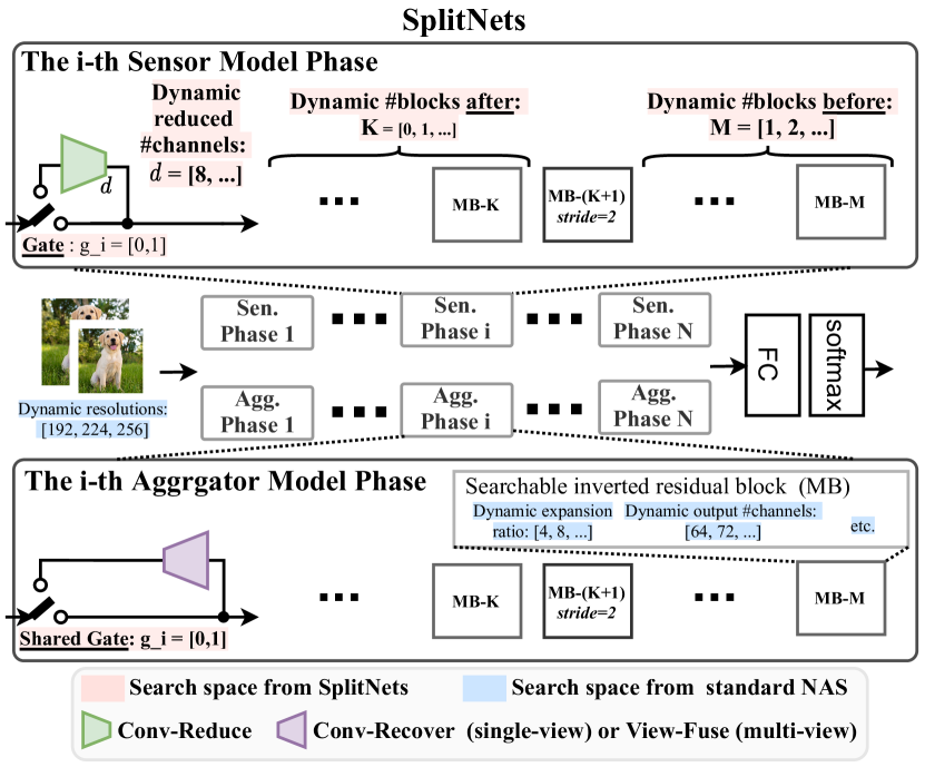
The splitting module for single-view tasks consists of two parts, Conv-Reduce and Conv-Recover, which will be discussed in  Section 3.1.3 for their architectures and initialization strategy. The splitting module could be inserted after any of inverted residual block (MB) in a supernet theoretically. However, instead of equipping every MB with a candidate splitting module, we divide a supernet into several phases and insert one splitting module for each phase to reduce the number of splitting positions to be optimized.

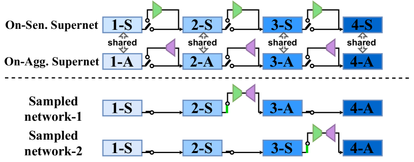
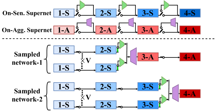
Suppose a supernet has $N$ stride-2 MB blocks, We divide the whole model into $N$ phases where each phase has one stride-2 MB block. Within a phase, MB blocks before the stride-2 block have the same spatial size and similar channel sizes. We then insert one Conv-Reduce (green trapezium, Figure 3) layer $\phi:\mathbb{R}^{c\times s\times s}\rightarrow\mathbb{R}^{d\times s\times s}$ in each phase for the on-sensor supernet, associated with a gate variable ${\textnormal{g}}_{i}\in\{0,\leavevmode\nobreak\ 1\}$ indicating whether this layer is selected. A corresponding Conv-Recover (purple trapezium, Figure 3) layer $\phi^{\prime}:\mathbb{R}^{d\times s\times s}\rightarrow\mathbb{R}^{c\times s\times s}$ will be inserted into the on-aggregator supernet. Conv-Recover layer shares the same gate variable with Conv-Reduce, meaning that they are always selected, or not, at the same time. Using Conv-Recover allows weight-sharing of a block between different sampled sub-networks specified by different Conv-Reduce selections during training.

The number of MB blocks before (variable $M$) and after (variable $K$) the splitting module can be adjusted freely and searched through SA-NAS. This provides us with full search space of the splitting point at fine granularity, as well as a small amount of candidate networks to train. In particular, on-sen. and on-agg. blocks at the same depth learn similar features and can share weights for single-view problems.

In sub-network sampling, once a splitting module (i.e., $g_{i}=1$) is selected, we take blocks before splitting from the on-sensor supernet and blocks after splitting from the on-aggregator supernet, and stitch them together using splitting module as the joint point to form a sampled network as illustrated in Figure 4.

Eventually, we need exactly one splitting module. Therefore, gate vector ${\mathbf{g}}=\left({\textnormal{g}}_{1},\dots,{\textnormal{g}}_{M}\right)$ is restricted to a one-hot vector in the resource-constrained architecture search stage. However, during supernet training, we are free to insert more splitting modules to help reduce the maximum performance loss (see  Appendix D).

Figure 5: SA-NAS for multi-view SplitNets. A convolution layer (Conv-Reduce, purple trapezium) to reduce input’s channel size on the sensor side. The reduced input from $V$ views will be concatenated together (View-Fuse, green trapezium) on the aggregator. In this example, 3-A and 3-S are learning features for local view and mixed views respectively, thus their weights cannot be shared.

3.1.2 SA-NAS for Multi-View SplitNets

With $V$ sensors in the system, $V$ images are captured from different perspectives. Each sensor processes its captured image with the on-sen. model. Afterwards, a fusion module on the aggregator will fuse the compressed $V$ features from sensors and the on-agg. model further transforms the fused features to the final result.

Similar to searching the position of splitting module (i.e., Conv-Reduce and Conv-Recover) for single-view tasks, we now use SA-NAS to search the position of splitting module (i.e., Conv-Reduce and View-Fuse) for multi-view tasks. Compared with single-view case, we keep the Conv-Reduce layers in the on-sen. supernet, but replace the Conv-Recover layers in the on-agg. supernet with View-Fuse layers to aggregate features across multiple views as illustrated in Figure 5.

Different from single-view case, no weight sharing can be performed between the on-sen. and on-agg. supernets because on-agg. network learns to process fused representation which contains mixed information from $V$ views, while on-sen. supernet processes only local information. In other words, blocks on-sen. and on-agg. have radically different functionalities, and it is sub-optimal to enforce a shared block to play these two roles simultaneously.

3.1.3 Architecture of Splitting Module

Single-View: Reduce and Recover Inspired by  [11, 46, 36, 4, 45], we adopt a straight-forward implementation for the splitting module in SA-NAS. As illustrated in Figure 3, we use two convolution layers to compress features: $\phi:\mathbb{R}^{c\times s\times s}\rightarrow\mathbb{R}^{d\times s\times s}$ and recover features: $\phi^{\prime}:\mathbb{R}^{d\times s\times s}\rightarrow\mathbb{R}^{c\times s\times s}$ on channel dimension, where $d$ can be searched by SA-NAS. In SA-NAS, $\phi$ and $\phi^{\prime}$ are always selected simultaneously.

Multi-View: Reduce and Fuse Prior work has proposed intricate fusion architecture like recurrent and graph neural networks targeting different applications [49, 34, 20, 16].

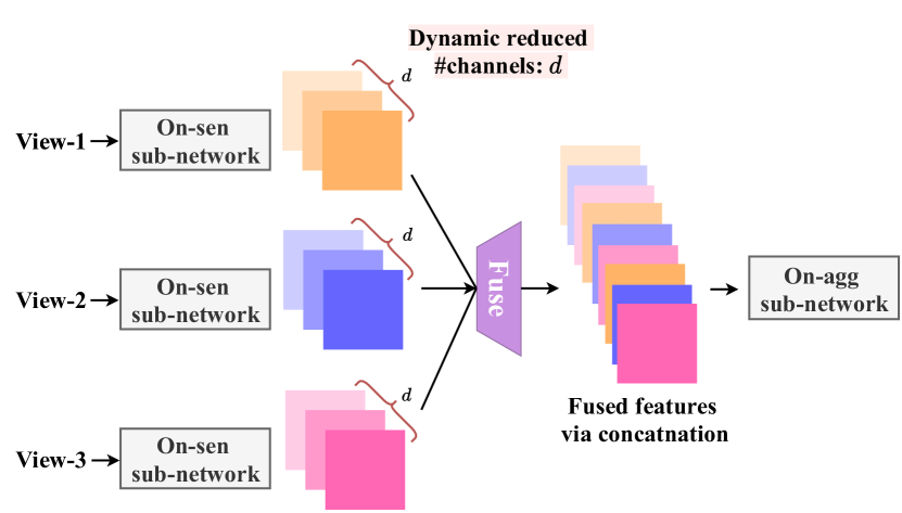
Similar to the single-view, multi-view splitting module uses a convolution layer $\phi:\mathbb{R}^{c\times s\times s}\rightarrow\mathbb{R}^{d\times s\times s}$ for communication saving, and then fuses these reduced features from $V$ views together with the View-Fuse layer. Without loss of generality, we use a highly simplified fusion operation - concatenation (See Appendix B). View-Fuse will concatenate $V$ views together along the channel dimension $\texttt{concat}\left(V\times\mathbb{R}^{d\times s\times s}\right)\rightarrow\mathbb{R}^{V\cdot d\times s\times s}$.

Despite of the extreme simplicity of fusion architecture, we empirically show that searching the splitting (i.e., fusion) position jointly with network architecture using SA-NAS achieves considerable accuracy improvement, compared with SOTA approaches with dedicated fusion layers (see Section 4).

Initialization Method	Weights’ Variance	Average
Kaiming Fan-In or -Out [21]	${\frac{2}{k^{2}\cdot{{c_{\mathrm{in}}}}}}$ or ${\frac{2}{k^{2}{{c_{\mathrm{out}}}}}}$	No
Xavier [17]	${\frac{2}{k^{2}\cdot{{(c_{\mathrm{in}}+c_{\mathrm{out}})/2}}}}$	Arithmetic
Ours	${\frac{2}{k^{2}{{\sqrt{c_{\mathrm{in}}\cdot c_{\mathrm{out}}}}}}}$	Geometric

Table 3: Comparison of different initialization approaches. Equations in this table assume the activation function as ReLU.

Split-aware Weights Initialization As is also observed by  [36], adding compression / fusion modules into supernet training process degrades the training stability and yields suboptimal training performance. We find that the issue is caused by the gradient of the compression module. In practice, the gradients of the compression layer are $>$10$\times$ bigger than regular layers, starting from initialization.

Take Kaiming initialization as an example [21]. Its Fan-In mode is to ensure that the output of each layer has zero mean and unit variance , so the output magnitude will not explode in the forward pass. Similarly, the backward pass of a convolution layer is also a convolution but with the transposed weight matrix ${\mathbf{W}}^{T}$, and applying the same idea will lead to Fan-Out mode .

Either Fan In or Fan Out works well for standard neural architectures because most of layers’ input channel size $c_{\mathrm{in}}$ and output channel size $c_{\mathrm{out}}$ are similar (see Table 3). However, for Conv-Reduce and Conv-Recover, $c_{\mathrm{in}}$ and $c_{\mathrm{out}}$ are very different, thus Kaiming and Xavier cannot reconcile both forward and backward at the same time.

In order to mitigate this conflict, we use a new initialization strategy by replacing $c_{\mathrm{in}}$ or $c_{\mathrm{out}}$ with their geometic average $\sqrt{c_{\mathrm{in}}\cdot c_{\mathrm{out}}}$. Using geometric average allows us to find a better compromise between forward and backward passes and significantly improve training stability and final accuracy as shown in Appendix F.

3.2 Resource-constrained searching (Stage 2)

After the supernet training stage, all candidate networks are fully optimized. The next step is to search the optimal network which satisfies system constraints. Since two-stage NAS decouples the training and searching, the system constraints are fully configurable. In addition, one does not have to redo the costly supernet training when the system constraints change.

Since the searching space of supernet is extremely huge, evolution algorithm is adopted to accelerate the searching process [60, 18, 7, 5, 55]. Specifically, we mutate and crossover pairs of current generation’s networks to generate their children networks. All children networks are evaluated and selected according to their hardware and task performance. The selected children networks will be used to populate candidate networks for the next generation. After several generations, optimal networks can be found.

We consider two kinds of hardware constraints simultaneously. 1) Soft constraints, such as overall latency under the same task accuracy: Children networks with top-$k$ smallest latency’s will be selected. 2) Hard constraints, such as peak memory usage: Regardless of accuracy and performance, only children networks that satisfy all hard constraints can be selected to the next generation.

Figure 6: Hardware model for the target system. On-sensor compute uses a less advanced technology node (16nm) with limited on-chip memory. Smart sensors are connected to an aggregator using a shared 1.2 Gb/s bus. Aggregator uses advanced process (7nm) and has faster compute with larger memory.

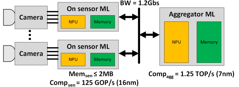
System Hardware Modeling Given a sampled network, its hardware performance is modeled through a hardware simulator. In this work, we use a hardware simulator customized for a realistic HMD system [40, 61] with smart sensors (see Figure 6). The on-sensor processor is equipped with a 16nm neural processing unit (NPU) with peak performance of $\operatorname{Comp}_{\texttt{sen}}=125$ GOP/s and peak memory of $\operatorname{Mem}_{\texttt{sen}}=2$ MB. The aggregator processor is modeled with a powerful 7nm NPU with peak performance of $\operatorname{Comp}_{\texttt{agg}}=1.25$ TOP/s and sufficient on-chip memory. The communication between the sensors and the aggregator is modeled with a high-performance shared bus for HMD with peak bandwidth of $\operatorname{BW}_{\texttt{comm}}=1.2$ Gbs. The high speed bus will be shared between multiple sensors in practice. More implementation details are summarized in the appendix.

4 Results

We validate that SplitNets can satisfy all system hardware constraints and find an optimized model with competitive accuracy and the best system performance compared with SOTA models crafted by hands or searched by standard NAS methods. Specifically, we evaluate our SplitNets for single-view system on ImageNet classification (Section 4.1) and SplitNets for multi-view system on 3D classification (Section 4.2).

Figure 7: Left: Comparison of SplitNets with prior approaches using different network architectures on ImageNet from Table 4. Right: Visualization of SplitNets searched models’ accuracy (dashed line and the right y-axis) and overall latency breakdown (the stacking bar plot and the left y-axis). Each searched model’s overall latency is represented by a vertical stacked bar. From bottom to top of each bar, the length’s of three colors represent $T_{\texttt{sen}},\leavevmode\nobreak\ T_{\texttt{comm}},\leavevmode\nobreak\ T_{\texttt{agg}}$ respectively.

HW Constraints

Method

Backbone

Top-1

On-sensor

Comm.

On-aggregator

Overall Latency

#Params

#OPs

Peak

Latency

Size

Latency

#Params

#OPs

Latency

$\operatorname{Mem}_{\texttt{sen}}$ $\leq$ 2MB $\operatorname{Comp}_{\texttt{sen}}$ (16nm) = $\mathbf{125}$ GOP/s $\operatorname{Comp}_{\texttt{agg}}$ (7nm) = $\mathbf{1.25}$ TOP/s $\operatorname{BW}_{\texttt{comm}}$ = 37.5 MB/s $*$: For all models, We assume weights and activation are quantized to 8-bit without loss of accuracy.

All-on-sen.

MobileNet-v2

71.88

3.51M

301M

5.90MB

2.46ms

0

0

0

0

0

2.46ms

MNASNet-1.0§

73.46

4.38M

314M

5.59MB

2.52ms

0

0

0

0

0

2.52ms

EfficientNet-B0§

77.13

5.30M

386M

7.70MB

3.09ms

0

0

0

0

0

3.09ms

ResNet-152

78.31

60.2M

11.5G

120 MB

92.1ms

0

0

0

0

0

92.1ms

RegNetX-3.2GF§

78.36

15.3M

3.18G

29.3MB

25.4ms

0

0

0

0

0

25.4ms

All-on-agg.

MobileNet-v2

71.88

0

0

0

0

$3\cdot 224^{2}$

4.01ms

3.51M

301M

0.24ms

4.25ms

MNASNet-1.0§

73.46

0

0

0

0

$3\cdot 224^{2}$

4.01ms

4.38M

314M

0.25ms

4.26ms

EfficientNet-B0§

77.13

0

0

0

0

$3\cdot 224^{2}$

4.01ms

5.3M

386M

0.31ms

4.32ms

ResNet-152

78.31

0

0

0

0

$3\cdot 224^{2}$

4.01ms

60.2M

11.5G

9.21ms

13.2ms

RegNetX-3.2GF§

78.36

0

0

0

0

$3\cdot 224^{2}$

4.01ms

15.3M

3.18G

2.54ms

6.60ms

Neurosurgeon

MobileNet-v2

71.88

0

0

0

0

$3\cdot 224^{2}$

4.01ms

3.51M

301M

0.24ms

4.25ms

MNASNet-1.0§

73.46

82.0K

103 M

1.29MB

0.83ms

$80\cdot 14^{2}$

0.84ms

4.30M

212M

0.17ms

1.82ms

EfficientNet-B0§

77.13

0

0

0

0

$3\cdot 224^{2}$

4.01ms

5.3M

386M

0.31ms

4.32ms

ResNet-152

78.31

0

0

0

0

$3\cdot 224^{2}$

4.01ms

60.2M

11.5G

9.21ms

13.2ms

RegNetX-3.2GF§

78.36

0

0

0

0

$3\cdot 224^{2}$

4.01ms

15.3M

3.18G

2.54ms

6.60ms

Head Distill

ResNet-152†

75.13$\bm{\downarrow}$

12.8K

125M

0.82MB

1.00ms

$12\cdot 29^{2}$

0.27ms

60.8M

11.8G

9.45ms

10.72ms

DenseNet-169†

72.03$\bm{\downarrow}$

12.8K

125M

0.82MB

1.00ms

$12\cdot 29^{2}$

0.27ms

14.9M

3.27G

2.61ms

3.88ms

Inception-v3†

75.78$\bm{\downarrow}$

12.8K

223M

1.45MB

1.78ms

$12\cdot 38^{2}$

0.46ms

24.1M

5.03G

4.02ms

6.26ms

SplitNets

A§

73.15

93.4K

63.7M

0.68MB

0.51ms

$18\cdot 12^{2}$

0.07ms

6.73M

372M

0.30ms

0.88ms

B§

73.45

0.12M

70.5M

1.00MB

0.56ms

$18\cdot 12^{2}$

0.07ms

7.43M

402M

0.32ms

0.95ms

C§

76.98

92.8K

98.6M

1.14MB

0.79ms

$18\cdot 16^{2}$

0.13ms

7.63M

727M

0.58ms

1.49ms

D§

77.42

208K

137 M

1.52MB

1.10ms

$18\cdot 16^{2}$

0.13ms

7.85M

831M

0.66ms

1.88ms

E§

78.56

211K

214 M

1.54MB

1.71ms

$18\cdot 18^{2}$

0.16ms

7.85M

1050M

0.84ms

2.71ms

F§

78.91

98.0K

194 M

1.76MB

1.55ms

$32\cdot 36^{2}$

1.11ms

8.13M

1.18G

0.94ms

3.59ms

Table 4: Overall latency comparison on single-sensor system for ImageNet classification task. Green (or red) numbers mean the on-sensor memory consumption is less (or more) than a sensor’s memory constraint. ^§: The backbone model is from NAS methods.  ^†: The model, splitting point and accuracy are directly from “Head Distill” [36].

Method	Backbone	#Params	#OPs	Fusion			Top-1
				Position	Feature size	Arch.
MVCNN-su	VGG-M	90.5M	34.6G	Last Conv	$512\cdot 13^{2}$	View-Pool	81.1
MVCNN-su	MobileNet-v3	2.54M	661M	Last Conv	$576\cdot\leavevmode\nobreak\ 7^{2}$	View-Pool	86.0
MVCNN-su	MNASNet-0.5	2.22M	1.24G	Last Conv	$1280\cdot 7^{2}$	View-Pool	91.4
MVCNN-su	EfficientNet-B0	5.29M	4.62G	Last Conv	$1280\cdot 7^{2}$	View-Pool	92.1
MVCNN-new	VGG-11	132 M	90.0G	Last Conv	$512\cdot\leavevmode\nobreak\ 7^{2}$	View-Pool	88.7
MV-LSTM	ResNet-18	11.2M	21.9G	Last Conv	$512\cdot\leavevmode\nobreak\ 7^{2}$	Bi-LSTM	89.1
SeqViews	VGG-19	144M	235 G	Penultimate FC	$4096\cdot 1$	Bi-RNN	89.3
Auto-MVCNN	AM-c24	2.10M	3.20G	Last Conv	-	Searched	90.5
Auto-MVCNN	AM-c36	4.70M	6.90G	Last Conv	-	Searched	91.0
SplitNets	A	1.39M	513M	6-th (tot.   8) block	$16\cdot 6^{2}$	Concat.	92.3
SplitNets	B	2.44M	759M	8-th (tot. 13) block	$6\cdot 12^{2}$	Concat.	93.0
SplitNets	C	2.32M	1.83G	8-th (tot. 13) block	$6\cdot 14^{2}$	Concat.	93.8

Table 5: Performance comparison on multi-view 3D classification for MVCNN-su [48], MVCNN-new [49], MV-LSTM [34], SeqViews [20], Auto-MVCNN [31], and SplitNets. We assume that all models are not pre-trained on ImageNet.

Figure 8: We compare achieved accuracy as a function of the ratio, #OPs on one sen. / (#OPs on one sen. + #OPs on the agg.). Since prior methods conduct fusion around the final layer, their ratios are $\sim$1. In contrast, SplitNets are able to explore various positions and pick the best one.

4.1 Single-view Task: ImageNet

For the distributed computing with a single-view system, we use the public large-scale single-view classification dataset, ImageNet, to train and test the method and evaluate performance. Results are summarized in Table 4.

HW Constraints

Split

Backbone

Top-1

On-each-sensor

Comm.

On-aggregator

Overall Latency

#Params

#OPs

Peak

Latency

Size

Latency

#Params

#OPs

Latency

Sensor $\times$ 12 Aggregator $\times$ 1 $\operatorname{BW}_{\texttt{comm}}$ = 12.5 MB/s $*$: The others are same as as Table 4.

All-on-agg.

VGG-11

88.7

0

0

0

0

$3\cdot 224^{2}$

12.0ms

132 M

90.0G

73.2ms

84.9ms

ResNet-18

89.1

0

0

0

0

$3\cdot 224^{2}$

12.0ms

11.7M

21.8G

17.7ms

29.7ms

MobileNet-v3

86.0

0

0

0

0

$3\cdot 224^{2}$

12.0ms

2.55M

661M

0.58ms

12.6ms

MNASNet-0.5 †

91.4

0

0

0

0

$3\cdot 224^{2}$

12.0ms

2.22M

1.24G

1.01ms

13.0ms

EfficientNet-B0 †

92.1

0

0

0

0

$3\cdot 224^{2}$

12.0ms

5.29M

4.62G

3.76ms

15.8ms

Split at fusion

VGG-11

88.7

9.22M

7.49G

12.4MB

59.9ms

$512\cdot 7^{2}$

2.00ms

123M

123M

0.10ms

62.1ms

ResNet-18

89.1

11.2M

1.81G

12.8MB

14.5ms

$512\cdot 7^{2}$

2.00ms

0.51M

0.51M

0.40ns

16.5ms

MobileNet-v3

86.0

0.93M

54.9M

1.38MB

0.44ms

$576\cdot 7^{2}$

2.26ms

1.62M

1.62M

1.29ns

2.71ms

MNASNet-0.5§

91.4

0.94M

103M

1.54MB

0.83ms

$1280\cdot 7^{2}$

5.03ms

1.28M

1.28M

1.03ns

5.83ms

EfficientNet-B0§

92.1

4.01M

385M

6.42MB

3.08ms

$1280\cdot 7^{2}$

5.03ms

1.28M

1.28M

1.03ns

8.03ms

SplitNets

A§

92.3

0.14M

41.8M

0.06MB

0.33ms

$16\cdot 6^{2}$

0.05ms

1.25M

11.4M

0.01ms

0.39ms

B§

93.0

0.17M

58.7M

0.08MB

0.47ms

$6\cdot 12^{2}$

0.07ms

2.27M

55.4M

0.06ms

0.59ms

C§

93.8

0.18M

147M

0.11MB

1.17ms

$6\cdot 14^{2}$

0.09ms

2.15M

73.3M

0.07ms

1.34ms

Table 6: Overall latency comparison on a multi-sensor system with a 3D classification task. Since 12 sensors are assumed in this task, each sensor is allocated 12.5MB/s bandwidth. Green (or red) numbers mean the on-sensor memory consumption is less (or more) than a sensor’s memory constraint. ^§: The backbone model is from NAS methods.

SplitNets training / searching configurations In supernet training, we sample 5 kinds of networks (see  Appendix D) and optimize for 360 epochs with batch size 4096 using the standard training receipt from [54]. In resource-constrained searching, we sample 512 candidate networks with 20 generations using evolution algorithm [9, 54, 55].

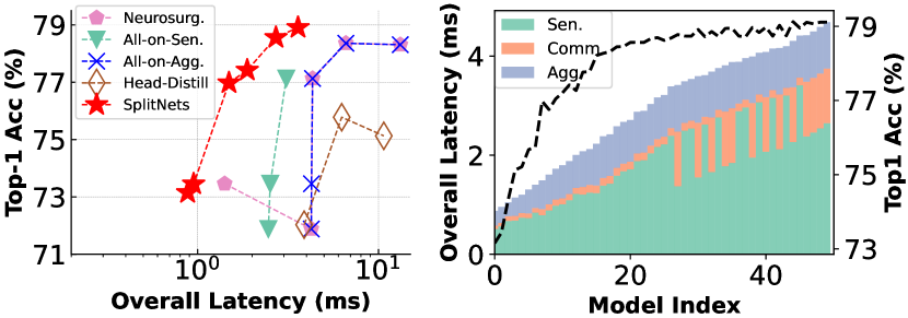
Comparing SplitNets against SOTA Methods we compare SplitNets against several existing models which are handcrafted or searched by existing NAS methods. The compared models include MobileNet-v2 [44], MNASNet [52], EfficientNet [53], ResNet [22], DenseNet [25], Inception-v3 [51], and RegNet [41], where the first three architectures are specifically designed for mobile on-device computing. To make the evaluation more realistic to real-time applications [32], we assume each of the four sensors is allocated 25% bandwidth of the shared bus. We also assume that all models’ weights and activation are quantized to 8-bit without accuracy degradation. (And literature has shown this assumption is reasonable. [56, 30, 12, 15]) If models have larger bitwidth, SplitNets will benefit more because the communication saving from feature compression is more pronounced.

We compare SA-NAS approach with four baseline model split methods:

• “All-on-sen.”: All computation happens on the sensor. The communication overhead is negligible but the peak memory often exceeds sensor’s memory capacity. In our experiments, we discover that all existing models, even lightweight ones, require $>$5MBs peak memory, which are too large for on-sensor deployment.

• “All-on-agg.”: Transmit raw image to aggregator and perform all computation on aggregator. Communication becomes the bottleneck, and the system is not scalable with increasing number of sensors.

• “Neurosurgeon [28]”: a heuristic method which profiles each layer and exhaustively searches every possible splitting position to find the optimal partition. Neurosurgeon performs the model split for many networks and finds that the optimal split often falls in the beginning or the last layer, which degenerates to “All-on-agg.” or “All-on-sen.”. We apply “Neurosurgeon [28]” on recent efficient architectures and observe similar results. This validates the necessity of joint designing network and the split.

• “Head Distill [23]”: a method that first manually determines the position of splitting point and then replaces the head part with a smaller networks through knowledge distillation. This approach is able to significantly reduce the communication cost compared with “All-on-agg.” and satisfy the hardware constraints. However, “Head Distill [23]” introduces 1.5%-3.6% accuracy drop even for parameter-redundant architectures like ResNet-152, DenseNet-169, and Inception-v3. Also, exhaustively searching the splitting point and hyper-parameters of the on-sen. network in  [23] also requires redoing the costly training, which is inefficient for deployment.

In the bottom of Table 4, we report a series of networks searched by SA-NAS. Under different accuracy targets, SplitNets consistently outperforms prior methods (“Neurosurgeon” [28] and “Head Distill” [23]) on overall latency while satisfying all hardware constraints. In addition, SplitNets are able to balance the workload of sensor and aggregator and make trade-off among communication, accuracy and computation when system hardware configuration changes (See  Appendix H).

4.2 Multi-view Task: 3D Classification

Figure 9: Left: Accuracy (stars and the right y-axis) and overall latency breakdown (the stacking bar plot and the left y-axis) of searched networks by SplitNets. Each searched model’s overall latency is represented by a vertical stacked bar. From bottom to top of each bar, the length’s of three colors represent $T_{\texttt{sen}},\leavevmode\nobreak\ T_{\texttt{comm}},\leavevmode\nobreak\ T_{\texttt{agg}}$ respectively. Right: Visualization of three searched networks by SplitNets. The length of vertical lines represents the output channel size of a convolution layer. Dash means that the stride size is two. The green and purple trapezoids are Conv-Reduce and View-Fuse. Among the three networks, the first and third networks conduct fusion either too ‘late’ or too ‘early’, leading sub-optimal task and system performance.

We also evaluate SplitNets on a multi-view system with 3D Warehouse classification dataset that consists of 3D CAD models from 40 categories. CAD models in this benchmark come from 3D Warehouse [1]. Each 3D object is captured from 12 different views by 12 sensors, where each view is a 2D image of size $3\times 224\times 224$.

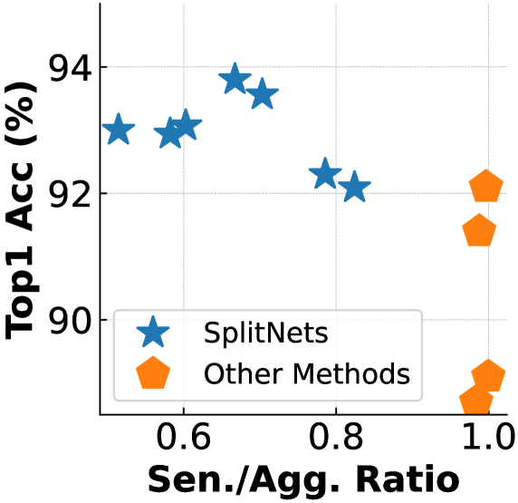
Searching Fusion Module’s Position Benefits Accuracy In Table 5, we compare the task performance of SplitNets models against existing models with various backbones [47, 52, 24, 53, 22] with dedicated fusion modules [31]. We assume all models are trained from scratch. Prior methods do not have the flexibility in adjusting the position of fusion module, and typically fuse features after the last convolution. SplitNets are able to explore all possible fusion positions (Figure 9, Right) and learn to pick the optimal split. Despite of the simplicity of fusion used, SplitNets significantly outperforms prior methods with fewer parameters and less computation.

Superior Overall Latency with SOTA Accuracy We further demonstrate the benefits of SplitNets for distributed computing on a 12-sensor system in Table 6. Compared to single-view system, multi-view system has heavier communication burden because multiple sensors have to share a single serial communication bus. As a result, the communication advantage of SplitNets is more pronounced. We visualize networks found by SplitNets in Figure 9. The position of fusion module keeps changing given different latency and accuracy targets. Interestingly, the best accuracy is not strictly correlated with the largest model which further validates the necessity of searching the best model instead of increasing model size.

5 Conclusion and Discussion

In summary, we introduce SplitNets with SA-NAS for efficient partition and inference of ML models on-device with distributed smart sensors. The proposed SA-NAS approach enables end-to-end model search with flexible positioning of a splitting module for single-view and multi-view problems. The resource-constrained searching successfully identifies model architectures that reduce overall system latency, satisfy hardware constraints, while maintaining high accuracy. Empirical results on ImageNet (single-view) and 3D Classification (multi-view) show that our approach can discover SOTA network architectures and model splitting solutions for distributed computing systems on AR/VR glasses.

Limitations and future work. The hardware model we adopt leverages an analytical model combing different hardware modalities, which are calibrated separately. Full system simulation with cycle accurate hardware models could be deployed for more precise latency evaluation.

Appendix A Multi-View Classification Dataset

We also evaluate SplitNets on a multi-view system with 3D Warehouse classification dataset that consists of 12,311 CAD models from 40 categories. CAD models in this benchmark come from 3D Warehouse [1]. For each object, 12 views are obtained by rotating the object every 30 degrees along the gravity direction. Using multiple views is necessary to obtain high classification accuracy according to prior work [16]. We use the same training and testing split as in [57]. For our experiments, the reported metric is per-class accuracy.

Input Resolution		{192, 224, 256, 288}
Model Phase	Block	NAS Search Space		SA-NAS Search Space
Model Phase	Block	Channel	Expansion Ratio	Depth Before Split Module	Depth After Split Module	Reduced channel $d$ Module
-	Conv	{16,24}	{1}	-	-	-
Phase 1	MBConv-1	{16,24}	{1}	{2,3,4,5}	{1,2,3}	{4,6,8}
	MBConv-2	{24,32}	{4,5,6}
Phase 2	MBConv-3	{32,40}	{4,5,6}	{1,2,3}	{1,2,3}	{6,8,10}
Phase 3	MBConv-4	{64,72}	{4,5,6}	{1,2,3}	{4,5,6,7,8,9}	{10,14,18}
	MBConv-5	{112,120,128}	{4,5,6}
Phase 4	MBConv-6	{192,200,208,216}	{6}	{1,2,3,4}	{2,3,4,5,6}	{16,24,32}
	MBConv-7	{216,224}	{6}
-	MBPool	{1792,1984}	{6}	-	-	-

Table 7: The supernet architecture configuration and search spaces for single-view SplitNets on ImageNet.

Appendix B Interlacing Concatenation for View Fusion

In Section 3.1.3, we introduce a splitting module for multi-view systems, consisting of two layers Conv-Reduce and View-Fuse. Since we mainly focus on searching the position of View-Fuse (i.e., the position of splitting module), we introduce a simple fusion operation - concatenation. More specifically, we concatenate features from $V$ views in an interlacing way along the channel dimension as illustrated in Figure 10. In the interlacing concatenation, we first concatenate the first channel from $V$ views, then repeat the same operation for the second channels, and so on. We adopt interlacing concatenation because the number of channels of each view is dynamically sampled during training and interlacing concatenation guarantees that the $i$-th channel of the fused features is always from the $(i\ \textrm{mod}\ V)$-th view.

Appendix C Supernet Configuration

As we mentioned in Section 3, We build the supernet’s search spaces mainly based on [9, 54] with some extra search spaces from our SA-NAS as shown in Figure 3. Search spaces from standard NAS [9, 54] include number of layers, output channel size and expand ratio of each inverted residual block (MB). Following [9, 54], we use Swish as activation function. The supernet architecture configuration and search space for single-view SplitNets on ImageNet are summarized in Table 7.

Appendix D Sampling Strategy of Splitting Modules for Supernet Training

Figure 10: Illustration of interlacing concatenation. Interlacing concatenation guarantees that the $i$-th channel of the fused features is always from the $(i\ \textrm{mod}\ V)$-th view. In the example of this figure, $V=3$.

D.1 Single-View SplitNets

In supernet training, we jointly train multiple sub-networks sampled from the supernet at each iteration. Various sampling strategies can be used [5, 60, 9, 54]. For example, BigNAS [60] samples three kinds of networks: 1) the largest sub-network (“max”); 2) the smallest sub-network (“min”); 3) several randomly sub-sampled networks. Since the largest sub-network usually has better accuracy, it can be used as teacher to supervise other sub-networks via knowledge distillation losses [23]. Some variants of this “sandwich” sampling strategy are also proposed like sampling sub-networks according to their predicted accuracy [54].

Compared with previous work, we have different interests on sub-networks. Eventually, we want to find the optimal architecture with exact one splitting module. However, as an information bottleneck, splitting module will inevitably introduce accuracy degradation. During training, we aim to minimize this degradation by improving the accuacy lower bound. We insert multiple splitting modules to help sub-networks increase tolerance of splitting modules. Inspired by BigNAS [60] and AttentiveNAS [54], we sample five sub-networks per iteration to train jointly.

1. “Max with zero hot”: The largest sub-network without splitting module can be treated as the best Pareto architecture. Training this sub-network helps improve the accuracy upper bound of all sub-networks.

2. “Max with all hot”: The largest sub-network with all $N$ splitting modules contains all weights in the supernet. Training this sub-network ensures all weights are updated at least once per iteration.

3. “Min with zero hot”: The smallest sub-network without splitting module contains weights which are shared across all sub-networks. Training this sub-network helps the optimization of the most frequently shared weights.

4. “Min with all hot”: The smallest sub-network with all $N$ splitting modules can be treated as the worst Pareto architecture. Training this sub-network helps improve the accuracy lower bound of the all sub-networks.

5. ‘Random with one hot”: A randomly sampled sub-network with exact one splitting module is the sub-network we are interested in during the second stage and final deployment.

Figure 11: Training curves of four different sub-networks sampled from the supernet for single-view SplitNets. “max” (or “min”) indicts the maximum (or “minimum”) sub-network sampled from the supernet. “all hot” (or “zero hot”) means that the sampled sub-network contains all possible (or none of) splitting modules. The drop of performance introduced (green line against orange line and blue line against magenta line) by inserting splitting module is mitigated. The red triangles are sampled sub-networks with one splitting module (i.e., “Random with one hot”). The green and pink lines can be treated as the upper and lower bounds of sub-networks.

Figure 12: Comparison between our new sampling strategy (solid lines) and baseline “sandwich” sampling strategy (dashed lines) for single-view SplitNets as elaborated in Section D.1. Our new sampling strategy helps reduce accuracy drop in SplitNets due to splitting modules. For example, the discrepancy between solid blue and pink lines is significantly smaller than discrepancy between dashed blue and pink lines.

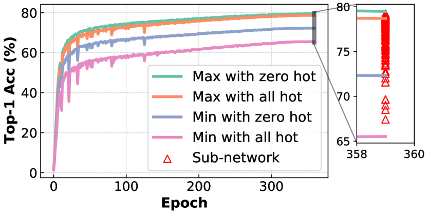
We visualize training curves of aforementioned sub-networks in Figure 11. The red triangles are some sampled sub-networks with one splitting module. Their accuracy is bounded by the “Max with zero hot” and “Min with all hot” sub-networks.

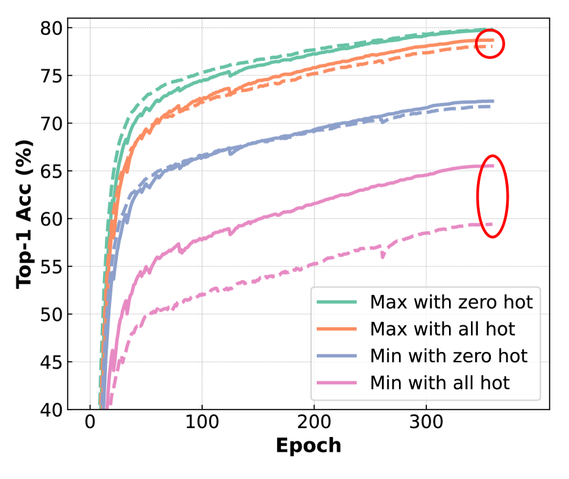
In addition, we compare our new sampling strategy against the baseline “sandwich” sampling strategy, which replaces “Max with all hot” (and “Min with all hot”) with “Max with one hot” (and “Min with one hot”) during supernet training. From Figure 12, we find that sampling more than one splitting modules during training helps reduce accuracy drop introduced by splitting modules in SplitNets. For example, the discrepancy between solid blue and pink lines is significantly smaller than discrepancy between dashed blue and pink lines.

D.2 Multi-View SplitNets

For multi-view SplitNets, each splitting module contains a fusion operation which can only be performed once for one network. So we are not able to sample more than one splitting modules during neither supernet training nor architecture searching. We use the baseline “sandwich” sampling strategy for multi-view SplitNets.

Appendix E Analysis of Different Initializations

As we discussed in Section 3.1.3, both forward and backward passes of a convolution layer can be expressed by convolution operations. The goal of initialization is to ensure the magnitude of output (and gradient) does not explode during forward (and backward) pass as shown in the following two equations,

$$\texttt{CONV}_{\mathrm{forward}}\left({\mathbf{W}},{\mathbf{x}}_{l}\right)={\mathbf{y}}_{l}\sim\mathcal{N}(0,1)$$ (2)

$$\texttt{CONV}_{\mathrm{backward}}\left({\mathbf{W}}^{T},\frac{\partial\mathcal{L}}{\partial{\mathbf{y}}_{l}}\right)=\frac{\partial\mathcal{L}}{\partial{\mathbf{x}}_{l}}\sim\mathcal{N}(0,1),$$ (3)

where we assume the activation function as ReLU [22], ${\mathbf{x}}_{l+1}=\operatorname{max}({\mathbf{y}}_{l},0)$. Solving Equation 2 or Equation 3 leads to Kaiming Fan-In or Kaiming Fan-Out [21],

$${\mathbf{W}} \sim\mathcal{N}\left(0,\frac{2}{k^{2}\cdot c_{\mathrm{in}}}\right)\quad\quad\textsc{(Fan-In)}$$ (4)

$${\mathbf{W}} \sim\mathcal{N}\left(0,\frac{2}{k^{2}\cdot c_{\mathrm{out}}}\right)\quad\ \ \textsc{(Fan-Out)},$$ (5)

where $k$ is kernel size and $c_{\mathrm{in}}$ (and $c_{\mathrm{out}}$) is the input (and output) channel size.

In a splitting module, the difference between input and output channel sizes is usually enormous. For example, in a certain Conv-Reduce, we have $c_{\mathrm{in}}=256$ and $c_{\mathrm{out}}=8$. In this case, Fan-In mode’s weights variance is $\frac{256}{8}=32$ times larger than Fan-Out’s. Choosing either Fan-In or Fan-Out will cause the other one’s variance too large or too small. Although Xavier [17]’s arithmetic average of $c_{\mathrm{in}}$ and $c_{\mathrm{out}}$ may mitigate this issue, it is far from enough because arithmetic average between two numbers is dominated by the larger one, $0.5\cdot(256+8)\gg 8$.

Our split-aware initialization adopts geometric average instead of arithmetic average to make a better balance between forward and backward, $\sqrt{c_{\mathrm{in}}\cdot c_{\mathrm{out}}}$. In the next section, we empirically show that supernet training can benefit from our split-aware initialization.

Appendix F Empirical Comparison of Different Initializations

Figure 13: Accuracy comparison between Kaiming and our split-aware initalizations on the “Max with all hot” sub-network.

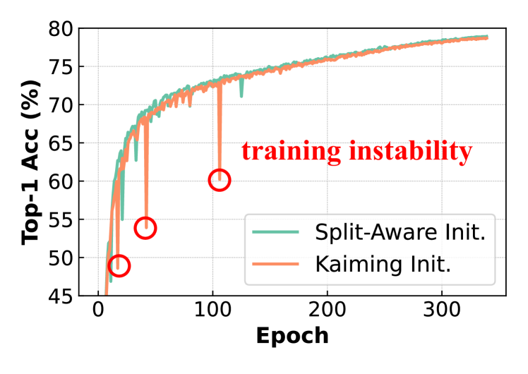
We compare our split-aware initialization against Kaiming initialization (Fan-In) on “Max with all hot” sub-network’s accuracy for ImageNet in Figure 13. Our split-aware initialization improves training stability as well as final accuracy (by 0.3%). In addition, if the base learning rate (0.05 in Figure 13) is slightly increased, conventional initialization will lead to divergence in training.

Appendix G Hardware Modeling

As discussed in Section 3.2, we use a hardware simulator customized for a realistic head mounted device. The on-sen. processor is equipped with a 16nm neural processing unit (NPU) with peak performance of $\operatorname{Comp}_{\texttt{sen}}=125$ GOP/s. So, the latency of on-sensor part (in Equation 1) can thus be approximately computed via $T_{\texttt{sen}}(f_{\texttt{sen}},{\mathbf{x}})=\operatorname{OP}(f_{\texttt{sen}},{\mathbf{x}})/\operatorname{Comp}_{\texttt{sen}}$, where $\operatorname{OP}(\cdot,\cdot)$ is the profiling function through cycle-accurate simulation for measuring the number of operations given model and input. In addition, the on-sen. processor’s peak memory is $\operatorname{Mem}_{\texttt{sen}}=2$ MB. Thus, the peak memory consumption of the on-sen part cannot exceed this peak memory constraint $M(f_{\texttt{sen}},{\mathbf{x}})\leq\operatorname{Mem}_{\texttt{sen}}$. When computing the peak memory consumption ($M(\cdot,\cdot)$), we consider the memory of both weights and activations: $M(f_{\texttt{sen}},{\mathbf{x}})=M_{\texttt{W}}(f_{\texttt{sen}})+M_{\texttt{A}}(f_{\texttt{sen}},{\mathbf{x}})$, where $M_{\texttt{W}}(f_{\texttt{sen}})$ is the memory consumption for storing all weights of $f_{\texttt{sen}}$ and $M_{\texttt{A}}(f_{\texttt{sen}},{\mathbf{x}})$ measures the peak memory consumption of activation taking residual connections into consideration. In this work, we consider homogeneous sensors which can represent most of AR/VR devices like Quest2 [2]. We leave the extension of SplitNets as a future work when heterogeneous sensors occur.

Appendix H Adaptability of SplitNets

Figure 14: Evolution of the best architectures when on-sen. processor’s peak computation performance increases. SA-NAS can automatically put more and wider layers on sensors.

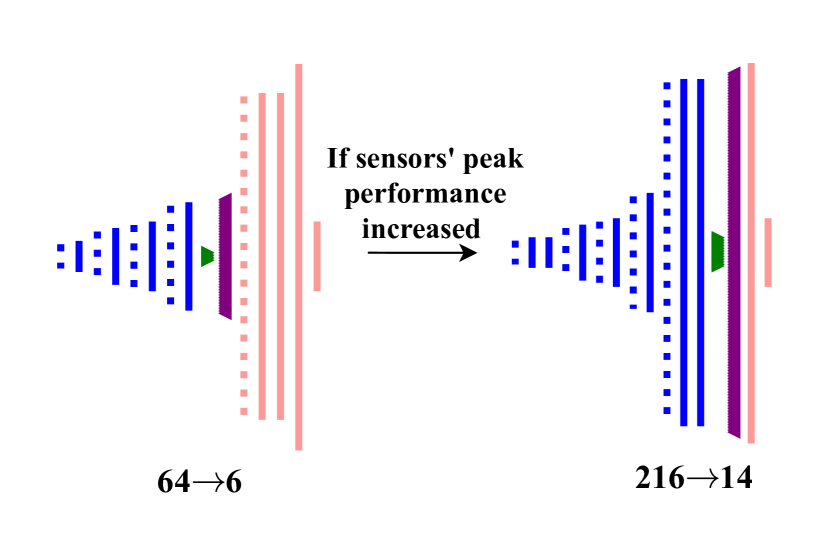
As we discussed in Section 3, two-stage NAS decouples the supernet training (stage 1) and architecture searching (stage 2). As a result, when the hardware configuration changes, one just needs to rerun the stage 2 without retraining the supernet. In this section, we change the hardware configuration and observe how the searched architectures evolve to fit the change of hardware configuration. Specifically, we increase the computation capability of on-sen. processors by four times and show the change of architectures with the best accuracy for the multi-view task in Figure 14. The left architecture is the best network for the default hardware configuration ($\operatorname{Comp}_{\texttt{sen}}=125$ GOP/s) from Table 6 (SplitNets-C). If on-sen. processors’ peak computation performance is increased by 4$\times$, SA-NAS can automatically put more and wider layers on-sen. and reduce the number of on-agg. layers to make a better trade-off. The network on the right achieves a better performance (94.0% top-1 accuracy) and lower latency (0.62 ms) compared with the left one.

References

- [1] 3d warehouse. https://3dwarehouse.sketchup.com/.
- [2] Oculus quest 2: Our most advanced new all-in-one vr headset.
- [3] Micheal Ambrash. Creating the future: Augmented reality, the next human-machine interface. pages 1–4, 2021.
- [4] Juliano S Assine, Eduardo Valle, et al. Single-training collaborative object detectors adaptive to bandwidth and computation. arXiv preprint arXiv:2105.00591, 2021.
- [5] Han Cai, Chuang Gan, Tianzhe Wang, Zhekai Zhang, and Song Han. Once for all: Train one network and specialize it for efficient deployment. In International Conference on Learning Representations, 2020.
- [6] Hyomin Choi and Ivan V Bajić. Deep feature compression for collaborative object detection. In 2018 25th IEEE International Conference on Image Processing (ICIP), pages 3743–3747. IEEE, 2018.
- [7] Xiangxiang Chu, Bo Zhang, and Ruijun Xu. Fairnas: Rethinking evaluation fairness of weight sharing neural architecture search. In Proceedings of the IEEE/CVF International Conference on Computer Vision, pages 12239–12248, 2021.
- [8] Robert A Cohen, Hyomin Choi, and Ivan V Bajić. Lightweight compression of neural network feature tensors for collaborative intelligence. In 2020 IEEE International Conference on Multimedia and Expo (ICME), pages 1–6. IEEE, 2020.
- [9] Xiaoliang Dai, Alvin Wan, Peizhao Zhang, Bichen Wu, Zijian He, Zhen Wei, Kan Chen, Yuandong Tian, Matthew Yu, Peter Vajda, and Joseph E. Gonzalez. Fbnetv3: Joint architecture-recipe search using neural acquisition function. CoRR, abs/2006.02049, 2020.
- [10] Amir Erfan Eshratifar, Mohammad Saeed Abrishami, and Massoud Pedram. Jointdnn: An efficient training and inference engine for intelligent mobile cloud computing services. IEEE Transactions on Mobile Computing, 2019.
- [11] Amir Erfan Eshratifar, Amirhossein Esmaili, and Massoud Pedram. Bottlenet: A deep learning architecture for intelligent mobile cloud computing services. In 2019 IEEE/ACM International Symposium on Low Power Electronics and Design (ISLPED), pages 1–6. IEEE, 2019.
- [12] Steven K Esser, Jeffrey L McKinstry, Deepika Bablani, Rathinakumar Appuswamy, and Dharmendra S Modha. Learned step size quantization. ICLR, 2020.
- [13] Abrash et al. Creating the future: Augmented reality, the next human-machine interface. IEEE IEDM, 2021.
- [14] Pinkham et al. Near-sensor dist. dnn processing for ar/vr. IEEE ESTCS, 2021.
- [15] Angela Fan, Pierre Stock, Benjamin Graham, Edouard Grave, Rémi Gribonval, Herve Jegou, and Armand Joulin. Training with quantization noise for extreme model compression. ICLR, 2021.
- [16] Yifan Feng, Zizhao Zhang, Xibin Zhao, Rongrong Ji, and Yue Gao. Gvcnn: Group-view convolutional neural networks for 3d shape recognition. In Proceedings of the IEEE Conference on Computer Vision and Pattern Recognition, pages 264–272, 2018.
- [17] Xavier Glorot and Yoshua Bengio. Understanding the difficulty of training deep feedforward neural networks. In Proceedings of the thirteenth international conference on artificial intelligence and statistics, pages 249–256. JMLR Workshop and Conference Proceedings, 2010.
- [18] Zichao Guo, Xiangyu Zhang, Haoyuan Mu, Wen Heng, Zechun Liu, Yichen Wei, and Jian Sun. Single path one-shot neural architecture search with uniform sampling. In European Conference on Computer Vision, pages 544–560. Springer, 2020.
- [19] Shangchen Han, Beibei Liu, Randi Cabezas, Christopher D Twigg, Peizhao Zhang, Jeff Petkau, Tsz-Ho Yu, Chun-Jung Tai, Muzaffer Akbay, Zheng Wang, et al. Megatrack: monochrome egocentric articulated hand-tracking for virtual reality. ACM Transactions on Graphics (TOG), 39(4):87–1, 2020.
- [20] Zhizhong Han, Mingyang Shang, Zhenbao Liu, Chi-Man Vong, Yu-Shen Liu, Matthias Zwicker, Junwei Han, and CL Philip Chen. Seqviews2seqlabels: Learning 3d global features via aggregating sequential views by rnn with attention. IEEE Transactions on Image Processing, 28(2):658–672, 2018.
- [21] Kaiming He, Xiangyu Zhang, Shaoqing Ren, and Jian Sun. Delving deep into rectifiers: Surpassing human-level performance on imagenet classification. In Proceedings of the IEEE international conference on computer vision, pages 1026–1034, 2015.
- [22] Kaiming He, Xiangyu Zhang, Shaoqing Ren, and Jian Sun. Deep residual learning for image recognition. In Proceedings of the IEEE conference on computer vision and pattern recognition, pages 770–778, 2016.
- [23] Geoffrey Hinton, Oriol Vinyals, and Jeff Dean. Distilling the knowledge in a neural network. arXiv preprint arXiv:1503.02531, 2015.
- [24] Andrew Howard, Mark Sandler, Grace Chu, Liang-Chieh Chen, Bo Chen, Mingxing Tan, Weijun Wang, Yukun Zhu, Ruoming Pang, Vijay Vasudevan, et al. Searching for mobilenetv3. In Proceedings of the IEEE/CVF International Conference on Computer Vision, pages 1314–1324, 2019.
- [25] Gao Huang, Zhuang Liu, Laurens Van Der Maaten, and Kilian Q Weinberger. Densely connected convolutional networks. In Proceedings of the IEEE conference on computer vision and pattern recognition, pages 4700–4708, 2017.
- [26] Mikolaj Jankowski, Deniz Gündüz, and Krystian Mikolajczyk. Joint device-edge inference over wireless links with pruning. In 2020 IEEE 21st International Workshop on Signal Processing Advances in Wireless Communications (SPAWC), pages 1–5. IEEE, 2020.
- [27] Hyuk-Jin Jeong, InChang Jeong, Hyeon-Jae Lee, and Soo-Mook Moon. Computation offloading for machine learning web apps in the edge server environment. In 2018 IEEE 38th International Conference on Distributed Computing Systems (ICDCS), pages 1492–1499. IEEE, 2018.
- [28] Yiping Kang, Johann Hauswald, Cao Gao, Austin Rovinski, Trevor Mudge, Jason Mars, and Lingjia Tang. Neurosurgeon: Collaborative Intelligence Between the Cloud and Mobile Edge. In Proceedings of the Twenty-Second International Conference on Architectural Support for Programming Languages and Operating Systems. ACM, 2017.
- [29] Guangli Li, Lei Liu, Xueying Wang, Xiao Dong, Peng Zhao, and Xiaobing Feng. Auto-tuning neural network quantization framework for collaborative inference between the cloud and edge. In International Conference on Artificial Neural Networks, pages 402–411. Springer, 2018.
- [30] Yuhang Li, Xin Dong, and Wei Wang. Additive powers-of-two quantization: An efficient non-uniform discretization for neural networks. ICLR, 2019.
- [31] Zhaoqun Li, Hongren Wang, and Jinxing Li. Auto-mvcnn: Neural architecture search for multi-view 3d shape recognition. arXiv preprint arXiv:2012.05493, 2020.
- [32] Chiao Liu, Andrew Berkovich, Qing Chao, Song Chen, Ziyun Li, Hans Reyserhove, Syed Shakib Sarwar, and Tsung-Hsun Tsai. Intelligent vision sensors for ar/vr. In Imaging Systems and Applications, pages ITu5G–1. Optical Society of America, 2020.
- [33] Chiao Liu, Andrew Berkovich, Song Chen, Hans Reyserhove, Syed Shakib Sarwar, and Tsung-Hsun Tsai. Intelligent vision systems–bringing human-machine interface to ar/vr. In 2019 IEEE International Electron Devices Meeting (IEDM), pages 10–5. IEEE, 2019.
- [34] Chao Ma, Yulan Guo, Jungang Yang, and Wei An. Learning multi-view representation with lstm for 3-d shape recognition and retrieval. IEEE Transactions on Multimedia, 21(5):1169–1182, 2018.
- [35] Yoshitomo Matsubara, Sabur Baidya, Davide Callegaro, Marco Levorato, and Sameer Singh. Distilled split deep neural networks for edge-assisted real-time systems. In Proceedings of the 2019 Workshop on Hot Topics in Video Analytics and Intelligent Edges, pages 21–26, 2019.
- [36] Yoshitomo Matsubara, Davide Callegaro, Sabur Baidya, Marco Levorato, and Sameer Singh. Head network distillation: Splitting distilled deep neural networks for resource-constrained edge computing systems. IEEE Access, 8:212177–212193, 2020.
- [37] Yoshitomo Matsubara, Marco Levorato, and Francesco Restuccia. Split computing and early exiting for deep learning applications: Survey and research challenges. arXiv preprint arXiv:2103.04505, 2021.
- [38] Raul Mur-Artal, Jose Maria Martinez Montiel, and Juan D Tardos. Orb-slam: a versatile and accurate monocular slam system. IEEE transactions on robotics, 31(5):1147–1163, 2015.
- [39] Daniele Jahier Pagliari, Roberta Chiaro, Enrico Macii, and Massimo Poncino. Crime: Input-dependent collaborative inference for recurrent neural networks. IEEE Transactions on Computers, 2020.
- [40] Guofang Qin and Guoliang Qin. Virtual reality video image classification based on texture features. Complexity, 2021, 2021.
- [41] Ilija Radosavovic, Raj Prateek Kosaraju, Ross Girshick, Kaiming He, and Piotr Dollár. Designing network design spaces. In Proceedings of the IEEE/CVF Conference on Computer Vision and Pattern Recognition, pages 10428–10436, 2020.
- [42] Esteban Real, Alok Aggarwal, Yanping Huang, and Quoc V Le. Regularized evolution for image classifier architecture search. In Proceedings of the aaai conference on artificial intelligence, volume 33, pages 4780–4789, 2019.
- [43] Esteban Real, Sherry Moore, Andrew Selle, Saurabh Saxena, Yutaka Leon Suematsu, Jie Tan, Quoc V Le, and Alexey Kurakin. Large-scale evolution of image classifiers. In International Conference on Machine Learning, pages 2902–2911. PMLR, 2017.
- [44] Mark Sandler, Andrew G. Howard, Menglong Zhu, Andrey Zhmoginov, and Liang-Chieh Chen. Mobilenetv2: Inverted residuals and linear bottlenecks. In 2018 IEEE Conference on Computer Vision and Pattern Recognition, CVPR 2018, Salt Lake City, UT, USA, June 18-22, 2018, pages 4510–4520. Computer Vision Foundation / IEEE Computer Society, 2018.
- [45] Marion Sbai, Muhamad Risqi U Saputra, Niki Trigoni, and Andrew Markham. Cut, distil and encode (cde): Split cloud-edge deep inference. In 2021 18th Annual IEEE International Conference on Sensing, Communication, and Networking (SECON), pages 1–9. IEEE, 2021.
- [46] Jiawei Shao and Jun Zhang. Bottlenet++: An end-to-end approach for feature compression in device-edge co-inference systems. In 2020 IEEE International Conference on Communications Workshops (ICC Workshops), pages 1–6. IEEE, 2020.
- [47] Karen Simonyan and Andrew Zisserman. Very deep convolutional networks for large-scale image recognition. In International Conference on Learning Representations, 2015.
- [48] Hang Su, Subhransu Maji, Evangelos Kalogerakis, and Erik Learned-Miller. Multi-view convolutional neural networks for 3d shape recognition. In Proceedings of the IEEE international conference on computer vision, pages 945–953, 2015.
- [49] Jong-Chyi Su, Matheus Gadelha, Rui Wang, and Subhransu Maji. A deeper look at 3d shape classifiers. In Proceedings of the European Conference on Computer Vision (ECCV) Workshops, pages 0–0, 2018.
- [50] Masanori Suganuma, Mete Ozay, and Takayuki Okatani. Exploiting the potential of standard convolutional autoencoders for image restoration by evolutionary search. In International Conference on Machine Learning, pages 4771–4780. PMLR, 2018.
- [51] Christian Szegedy, Vincent Vanhoucke, Sergey Ioffe, Jon Shlens, and Zbigniew Wojna. Rethinking the inception architecture for computer vision. In Proceedings of the IEEE conference on computer vision and pattern recognition, pages 2818–2826, 2016.
- [52] Mingxing Tan, Bo Chen, Ruoming Pang, Vijay Vasudevan, Mark Sandler, Andrew Howard, and Quoc V. Le. Mnasnet: Platform-aware neural architecture search for mobile. In IEEE Conference on Computer Vision and Pattern Recognition, CVPR 2019, Long Beach, CA, USA, June 16-20, 2019, pages 2820–2828. Computer Vision Foundation / IEEE, 2019.
- [53] Mingxing Tan and Quoc V. Le. Efficientnet: Rethinking model scaling for convolutional neural networks. In Kamalika Chaudhuri and Ruslan Salakhutdinov, editors, Proceedings of the 36th International Conference on Machine Learning, ICML 2019, 9-15 June 2019, Long Beach, California, USA, volume 97 of Proceedings of Machine Learning Research, pages 6105–6114. PMLR, 2019.
- [54] Dilin Wang, Meng Li, Chengyue Gong, and Vikas Chandra. Attentivenas: Improving neural architecture search via attentive sampling. In Proceedings of the IEEE/CVF Conference on Computer Vision and Pattern Recognition, 2021.
- [55] Hanrui Wang, Zhanghao Wu, Zhijian Liu, Han Cai, Ligeng Zhu, Chuang Gan, and Song Han. Hat: Hardware-aware transformers for efficient natural language processing. In Annual Conference of the Association for Computational Linguistics, 2020.
- [56] Kuan Wang, Zhijian Liu, Yujun Lin, Ji Lin, and Song Han. Haq: Hardware-aware automated quantization with mixed precision. In IEEE Conference on Computer Vision and Pattern Recognition (CVPR), 2019.
- [57] Zhirong Wu, Shuran Song, Aditya Khosla, Fisher Yu, Linguang Zhang, Xiaoou Tang, and Jianxiong Xiao. 3d shapenets: A deep representation for volumetric shapes. In Proceedings of the IEEE conference on computer vision and pattern recognition, pages 1912–1920, 2015.
- [58] Lingxi Xie and Alan Yuille. Genetic cnn. In Proceedings of the IEEE international conference on computer vision, pages 1379–1388, 2017.
- [59] Shuochao Yao, Jinyang Li, Dongxin Liu, Tianshi Wang, Shengzhong Liu, Huajie Shao, and Tarek Abdelzaher. Deep compressive offloading: Speeding up neural network inference by trading edge computation for network latency. In Proceedings of the 18th Conference on Embedded Networked Sensor Systems, pages 476–488, 2020.
- [60] Jiahui Yu, Pengchong Jin, Hanxiao Liu, Gabriel Bender, Pieter-Jan Kindermans, Mingxing Tan, Thomas Huang, Xiaodan Song, Ruoming Pang, and Quoc Le. Bignas: Scaling up neural architecture search with big single-stage models. In European Conference on Computer Vision, pages 702–717. Springer, 2020.
- [61] Lim Jia Zheng, James Mountstephens, and Jason Teo. Four-class emotion classification in virtual reality using pupillometry. Journal of Big Data, 7(1):1–9, 2020.
- [62] Zhao Zhong, Junjie Yan, Wei Wu, Jing Shao, and Cheng-Lin Liu. Practical block-wise neural network architecture generation. In Proceedings of the IEEE conference on computer vision and pattern recognition, pages 2423–2432, 2018.
- [63] Barret Zoph and Quoc V Le. Neural architecture search with reinforcement learning. arXiv preprint arXiv:1611.01578, 2016.
- [64] Barret Zoph, Vijay Vasudevan, Jonathon Shlens, and Quoc V Le. Learning transferable architectures for scalable image recognition. In Proceedings of the IEEE conference on computer vision and pattern recognition, pages 8697–8710, 2018.