FedCorr: Multi-Stage Federated Learning for Label Noise Correction

Abstract

Federated learning (FL) is a privacy-preserving distributed learning paradigm that enables clients to jointly train a global model. In real-world FL implementations, client data could have label noise, and different clients could have vastly different label noise levels. Although there exist methods in centralized learning for tackling label noise, such methods do not perform well on heterogeneous label noise in FL settings, due to the typically smaller sizes of client datasets and data privacy requirements in FL. In this paper, we propose FedCorr, a general multi-stage framework to tackle heterogeneous label noise in FL, without making any assumptions on the noise models of local clients, while still maintaining client data privacy. In particular, (1) FedCorr dynamically identifies noisy clients by exploiting the dimensionalities of the model prediction subspaces independently measured on all clients, and then identifies incorrect labels on noisy clients based on per-sample losses. To deal with data heterogeneity and to increase training stability, we propose an adaptive local proximal regularization term that is based on estimated local noise levels. (2) We further finetune the global model on identified clean clients and correct the noisy labels for the remaining noisy clients after finetuning. (3) Finally, we apply the usual training on all clients to make full use of all local data. Experiments conducted on CIFAR-10/100 with federated synthetic label noise, and on a real-world noisy dataset, Clothing1M, demonstrate that FedCorr is robust to label noise and substantially outperforms the state-of-the-art methods at multiple noise levels.

85(17.5,259.5) ©2022 IEEE. Personal use of this material is permitted. Permission from IEEE must be obtained for all other uses, in any current or future media, including reprinting/republishing this material for advertising or promotional purposes, creating new collective works, for resale or redistribution to servers or lists, or reuse of any copyrighted component of this work in other works.

1 Introduction

Federated learning (FL) is a promising solution for large-scale collaborative learning, where clients jointly train a machine learning model, while still maintaining local data privacy [26, 37, 20]. However, in real-world FL implementations over heterogeneous networks, there may be differences in the characteristics of different clients due to diverse annotators’ skill, bias, and hardware reliability [4, 38]. Client data is rarely IID and frequently imbalanced. Also, some clients would have clean data, while other clients may have data with label noise at different noise levels. Hence, the deployment of practical FL systems would face challenges brought by discrepancies in two aspects i): local data statistics [26, 21, 13, 5], and ii): local label quality [4, 38]. Although recent works explored the discrepancy in local data statistics in FL, and learning with label noise in centralized learning (CL), there is at present no unified approach for tackling both challenges simultaneously in FL.

The first challenge has been explored in recent FL works, with a focus on performance with convergence guarantees [22, 27]. However, these works have the common implicit assumption that the given labels of local data are completely correct, which is rarely the case in real-world datasets.

The second challenge can be addressed by reweighting [7, 4, 31] or discarding [36] those client updates that are most dissimilar. In these methods, the corresponding clients are primarily treated as malicious agents. However, dissimilar clients are not necessarily malicious and could have label noise in local data that would otherwise still be useful after label correction. For FL systems, the requirement of data privacy poses an inherent challenge for any label correction scheme. How can clients identify their noisy labels to be corrected without needing other clients to reveal sensitive information? For example, [38] proposes label correction for identified noisy clients with the guidance of extra data feature information exchanged between clients and server, which may lead to privacy concerns.

Figure 1: An overview of FedCorr, organized into three stages. Algorithm steps are numbered accordingly.

Label correction and, more generally, methods to deal with label noise, are well-studied in CL. Yet, even state-of-the-art CL methods for tackling label noise [18, 3, 30, 8, 9, 40, 33, 35], when applied to local clients, are inadequate in mitigating the performance degradation in the FL setting, due to the limited sizes of local datasets. These CL methods cannot be applied on the global sever or across multiple clients due to FL privacy requirements. So, it is necessary and natural to adopt a more general framework that jointly considers the two discrepancies, for a better emulation of real-world data heterogeneity. Most importantly, privacy-preserving label correction should be incorporated in training to improve robustness to data heterogeneity in FL.

In this paper, we propose a multi-stage FL framework to simultaneously deal with both discrepancy challenges; see Fig. 1 for an overview. To ensure privacy, we introduce a dimensionality-based filter to identify noisy clients, by measuring the local intrinsic dimensionality (LID) [11] of local model prediction subspaces. Extensive experiments have shown that clean datasets can be distinguished from noisy datasets by the behavior of LID scores during training [25, 24]. Hence, in addition to the usual local weight updates, we propose that each client also sends an LID score to the server, which is a single scalar representing the discriminability of the predictions of the local model. We then filter noisy samples based on per-sample training losses independently for each identified noisy client, and relabel the large-loss samples with the predicted labels of the global model. To improve training stability and alleviate the negative impact caused by noisy clients, we introduce a weighted proximal regularization term, where the weights are based on the estimated local noise levels. Furthermore, we finetune the global model on the identified clean clients and relabel the local data for the remaining noisy clients.

Our main contributions are as follows:

• We propose a general multi-stage FL framework FedCorr to tackle data heterogeneity, with respect to both local label quality and local data statistics.

• We propose a general framework for easy generation of federated synthetic label noise and diverse (e.g. non-IID) client data partitions.

• We identify noisy clients via LID scores, and identify noisy labels via per-sample losses. We also propose an adaptive local proximal regularization term based on estimated local noise levels.

• We demonstrate that FedCorr outperforms state-of-the-art FL methods on multiple datasets with different noise levels, for both IID and non-IID data partitions.

2 Related work

2.1 Federated methods

In this paper, we focus on three closely related aspects of FL: generation of non-IID federated datasets, methods to deal with non-IID local data, and methods for robust FL.

The generation of non-IID local data partitions for FL was first explored in [26], based on dividing a given dataset into shards. More recent non-IID data partitions are generated via Dirichlet distributions [13, 1, 31].

Recent federated optimization work mostly focus on dealing with the discrepancy in data statistics of local clients and related inconsistency issues  [21, 32, 1]. For instance, FedProx deals with non-IID local data, by including a proximal term in the local loss functions [21], while FedDyn uses a dynamic proximal term based on selected clients [1]. SCAFFOLD [15] is another method suitable for non-IID local data that uses control variates to reduce client-drift. In [13] and [27], adaptive FL optimization methods for the global server are introduced, which are compatible with non-IID data distributions. Moreover, the Power-of-Choice (PoC) strategy [6], a biased client selection scheme that selects clients with higher local losses, can be used to increase the rate of convergence.

There are numerous works on improving the robustness of FL; these include robust aggregation methods [31, 19, 7], reputation mechanism-based contribution examining [36], credibility-based re-weighting [4], distillation-based semi-supervised learning [14], and personalized multi-task learning [19]. However, these methods are not designed for identifying noisy labels. Even when these methods are used to detect noisy clients, either there is no mechanism for further label correction at the noisy clients [31, 19, 36, 7], or the effect of noisy labels is mitigated with the aid of an auxiliary dataset, without any direct label correction [4, 14]. One notable exception is [38], which carries out label correction during training by exchanging feature centroids between clients and server. This exchange of centroids may lead to privacy concerns, since centroids could potentially be used as part of reverse engineering to reveal non-trivial information about raw local data.

In contrast to these methods, FedCorr incorporates the generation of diverse local data distributions with synthetic label noise, together with noisy label identification and correction, without privacy leakage.

2.2 Local intrinsic dimension (LID)

Informally, LID [11] is a measure of the intrinsic dimensionality of the data manifold. In comparison to other measures, LID has the potential for wider applications as it makes no further assumptions on the data distribution beyond continuity. The key underlying idea is that at each datapoint, the number of neighboring datapoints would grow with the radius of neighborhood, and the corresponding growth rate would then be a proxy for “local” dimension.

LID builds upon this idea [12] via the geometric intuition that the volume of an $m$-dimensional Euclidean ball grows proportionally to $r^{m}$ when its radius is scaled by a factor of $r$. Specifically, when we have two $m$-dimensional Euclidean balls with volumes $V_{1}$, $V_{2}$, and with radii $r_{1}$, $r_{2}$, we can compute $m$ as follows:

$$\frac{V_{2}}{V_{1}}=\bigg{(}\frac{r_{2}}{r_{1}}\bigg{)}^{m}\Rightarrow m=\frac{\log(V_{2}/V_{1})}{\log(r_{2}/r_{1})}.\\$$ (1)

We shall now formally define LID. Suppose we have a dataset consisting of vectors in $\mathbb{R}^{n}$. We shall treat this dataset as samples drawn from an $n$-variate distribution $\smash{\overline{\mathcal{D}}}$. For any $x\in\mathbb{R}^{n}$, let $Y_{x}$ be the random variable representing the (non-negative) distance from $x$ to a randomly selected point $y$ drawn from $\smash{\overline{\mathcal{D}}}$, and let $F_{Y_{x}}(t)$ be the cumulative distribution function of $Y_{x}$. Given $r>0$ and a sample point $x$ drawn from $\smash{\overline{\mathcal{D}}}$, define the LID of $x$ at distance $r$ to be

$$\operatorname{LID}_{x}(r):=\lim_{\varepsilon\to 0}\frac{\log F_{Y_{x}}((1+\varepsilon)r)-\log F_{Y_{x}}(r)}{\log(1+\varepsilon)},\\$$

provided that it exists, i.e. provided that $F_{Y_{x}}(t)$ is positive and continuously differentiable at $t=r$. The LID at $x$ is defined to be the limit $\operatorname{LID}_{x}=\lim_{r\to 0}\operatorname{LID}_{x}(r)$. Intuitively, the LID at $x$ is an approximation of the dimension of a smooth manifold containing $x$ that would “best” fit the distribution $\smash{\overline{\mathcal{D}}}$ in the vincinity of $x$.

Estimation of LID: By treating the smallest neighbor distances as “extreme events” associated to the lower tail of the underlying distance distribution, [2] proposes several estimators of LID based on extreme value theory. In particular, given a set of points $\mathcal{X}$, a reference point $x\in\mathcal{X}$, and its $k$ nearest neighbors in $\mathcal{X}$, the maximum-likelihood estimate (MLE) of $x$ is:

$$\widehat{\text{LID}}(x)=-\bigg{(}\frac{1}{k}\smash{\sum_{i=1}^{k}}\log\frac{r_{i}(x)}{r_{max}(x)}\bigg{)}^{-1},$$ (2)

where $r_{i}(x)$ denotes the distance between $x$ and its $i$-th nearest neighbor, and $r_{max}(x)$ is the maximum distance from $x$ among the $k$ nearest neighbors.

3 Proposed Method

In this section, we introduce FedCorr, our proposed multi-stage training method to tackle heterogeneous label noise in FL systems (see Algorithm 1). Our method comprises three stages: pre-processing, finetuning and usual training. In the first stage, we sample the clients without replacement using a small fraction to identify noisy clients via LID scores and noisy samples via per-sample losses, after which we relabel the identified noisy samples with the predicted labels of the global model. The noise level of each client is also estimated in this stage. In the second stage, we finetune the model with a typical fraction on relatively clean clients, and use the finetuned model to further correct the samples for the remaining clients. Finally, in the last stage, we train the model via the usual FL method (FedAvg [26]) using the corrected labels at the end of the second stage.

Algorithm 1 FedCorr (Red and Black line numbers in the pre-processing stage refer to operations for clients and server, respectively.)

Inputs: $N$ (number of clients), $T_{1}$, $T_{2}$, $T_{3}$, $\mathcal{D}=\{\mathcal{D}_{i}\}_{i=1}^{N}$ (dataset), $w^{(0)}$ (initialized global model weights).
Output: Global model $f_{G}^{\text{final}}$

1:// Federated Pre-processing Stage

2:$(\hat{\mu}_{1}^{(0)},\dots,\hat{\mu}_{N}^{(0)})\leftarrow(0,\dots,0)$ // estimated noise levels

3:for $t=1$ to $T_{1}$ do

4:   $\mathcal{S}=$Shuffle$(\{1,\dots,N\})$

5:   $w_{inter}\leftarrow w^{(t-1)}$   // intermediary weights

6:   for $k\in\mathcal{S}$ do

7:      $w_{k}^{(t)}\leftarrow$ weights that minimize loss function (5)

8:      Upload weights $w_{k}^{(t)}$ and LID score to server    

9:   Update global model $w^{(t)}\leftarrow w_{inter}$

10:   Divide all clients into clean set $\mathcal{S}_{c}$ and noisy set $\mathcal{S}_{n}$ based on cumulative LID scores via GMM

11:   for noisy client $k\in\mathcal{S}_{n}$ do

12:      Divide $\mathcal{D}_{k}$ into clean subset $\mathcal{D}^{c}_{k}$ and noisy subset $\mathcal{D}^{n}_{k}$ based on per-sample losses via GMM

13:       $\hat{\mu}_{k}^{(t)}\leftarrow\frac{|\mathcal{D}^{n}_{k}|}{|\mathcal{D}_{k}|}$ // update estimated noise level

14:       $y_{k}^{(i)}\leftarrow\operatorname*{arg\,max}f(x_{k}^{(i)};w^{(i)})$, $\forall(x_{k}^{(i)},y_{k}^{(i)})\in\mathcal{D}_{k}^{n}$    

15:

16:// Federated Finetuning Stage

17:$\mathcal{S}_{c}\leftarrow\{k|k\in\mathcal{S},\mu_{k}<0.1\}$, $\mathcal{S}_{n}\leftarrow\mathcal{S}\setminus\mathcal{S}_{c}$.

18:for $t=T_{1}+1$ to $T_{1}+T_{2}$ do

19:   Update $w_{k}^{(t)}$ by usual FedAvg among clients in $\mathcal{S}_{c}$

20:for Noisy client $k\in\mathcal{S}_{n}$ do

21:    $y_{k}^{(i)}\leftarrow\operatorname*{arg\,max}f(x_{k}^{(i)};w^{(i)})$, $\forall(x_{k}^{(i)},y_{k}^{(i)})\in\mathcal{D}_{k}$

22:

23:// Usual Federated Learning Stage

24:for $t=T_{1}+T_{2}+1$ to $T_{1}+T_{2}+T_{3}$ do

25:   Update $w_{k}^{(t)}$ by usual FedAvg among all clients

26:return$f_{G}^{\text{final}}:=f(\cdot;w^{(T_{1}+T_{2}+T_{3})})$

3.1 Preliminaries

Consider an FL system with $N$ clients and an $M$-class dataset $\mathcal{D}=\{\mathcal{D}_{k}\}_{k=1}^{N}$, where each $\mathcal{D}_{k}=\{(x_{k}^{i},y_{k}^{i})\}_{i=1}^{n_{k}}$ denotes the local dataset for client $k$. Let $\mathcal{S}$ denote the set of all $N$ clients, and let $w^{(t)}_{k}$ (resp. $w^{(t)}$) denote the local model weights of client $k$ (resp. global model weights obtained by aggregation) at the end of communication round $t$. At the end of round $t$, the global model $f_{G}^{(t)}$ would have its weights $w^{(t)}$ updated as follows:

$$w^{(t)}\leftarrow\sum_{\smash{k\in\mathcal{S}_{t}}}\frac{\smash{|\mathcal{D}_{k}|}}{\sum_{i\in\mathcal{S}_{t}}|\mathcal{D}_{i}|}w_{k}^{(t)},$$ (3)

where $\mathcal{S}_{t}\subseteq\mathcal{S}$ is the subset of selected clients in round $t$.

For the rest of this subsection, we shall give details on client data partition, noise model simulation, and LID score computation. These are three major aspects of our proposed approach to emulate data heterogeneity, and to deal with the discrepancies in both local data statistics and label quality.

Data partition. We consider both IID and non-IID heterogeneous data partitions in this work. For IID partitions, the whole dataset $\mathcal{D}$ is uniformly distributed at random among $N$ clients. For non-IID partitions, we first generate an $N\times M$ indicator matrix $\Phi$, where each entry $\Phi_{ij}$ indicates whether the local dataset of client $i$ contains class $j$. Each $\Phi_{ij}$ shall be sampled from the Bernoulli distribution with a fixed probability $p$. For each $1\leq j\leq M$, let $\upsilon_{j}$ be the sum of entries in the $j$-th column of $\Phi$; this equals the number of clients whose local datasets contain class $j$. Let $\boldsymbol{q}_{j}$ be a vector of length $\upsilon_{j}$, sampled from the symmetric Dirichlet distribution with the common parameter $\alpha_{Dir}>0$. Using $\boldsymbol{q}_{j}$ as a probability vector, we then randomly allocate the samples within class $j$ to these $\upsilon_{j}$ clients. Note that our non-IID data partition method provides a general framework to control the variability in both class distribution and the sizes of local datasets (see Fig. 2).

Figure 2: Depiction of non-IID partitions for different parameters.

Noise model. To emulate label noise in real-world data, we shall introduce a general federated noise model framework. For simplicity, this work only considers instance-independent label noise. This framework has two parameters $\rho$ and $\tau$, where $\rho$ denotes the system noise level (ratio of noisy clients) and $\tau$ denotes the lower bound for the noise level of a noisy client. Every client has a probability $\rho$ of being a noisy client, in which case the local noise level for this noisy client is determined randomly, by sampling from the uniform distribution $\textit{U}(\tau,1)$. Succinctly, the noise level of client $k$ (for $k=1,\dots,N$) is

$$\mu_{k}=\begin{cases}u\sim\textit{U}(\tau,1),&\text{with probability }\rho;\\ 0,&\text{with probability }1-\rho.\end{cases}$$ (4)

When $\mu_{k}\neq 0$, the $100\cdot\mu_{k}\%$ noisy samples are chosen uniformly at random, and are assigned random labels, selected uniformly from the $M$ classes.

LID scores for local models. In this paper, we associate LID scores to local models. Consider an arbitrary client with local dataset $\mathcal{D}$ and current local model $f(\cdot)$. Let $\mathcal{X}:=\{f(x)\}_{\smash{x\in\mathcal{D}}}$ be the set of prediction vectors, and for each $x\in\mathcal{D}$, compute $\widehat{LID}(f(x))$ w.r.t. the $k$ nearest neighbors in $\mathcal{X}$, as given in (2). We define the LID score of $(\mathcal{D},f)$ to be the average value of $\widehat{LID}(f(x))$ over all $x\in\mathcal{D}$. Note that as the local model $f(\cdot)$ gets updated with each round, the corresponding LID score will change accordingly.

Experiments have shown that given the same training process, models trained on a dataset with label noise tend to have larger LID scores as compared to models trained on the same dataset with clean labels [25, 24]. Intuitively, the prediction vectors of a well-trained model, trained on a clean dataset, would cluster around $M$ possible one-hot vectors, corresponding to the $M$ classes. However, as more label noise is added to the clean dataset, the prediction vector of a noisy sample would tend to be shifted towards the other clusters, with different noisy samples shifted in different directions. Hence, the prediction vectors near each one-hot vector would become “more diffuse” and would on average span a higher dimensional space.

3.2 Federated pre-processing stage

FedCorr begins with the pre-processing stage, which iteratively evaluates the quality of the dataset of each client, and relabels identified noisy samples. This pre-processing stage differs from traditional FL in the following aspects:

• All clients will participate in each iteration. Clients are selected without replacement, using a small fraction.

• An adaptive local proximal term is added to the loss function, and mixup data augmentation is used.

• Each client computes its LID score and per-sample cross-entropy loss after local training and sends its LID score together with local model updates to the server.

Client iteration and fraction scheduling.
The pre-processing stage is divided into $T_{1}$ iterations. In each iteration, every client participates exactly once. Every iteration is organized by communication rounds, similar to the usual FL, but with two key differences: a small fraction is used, and clients are selected without replacement. Each iteration ends when all clients have participated.

It is known that large fractions could help improve the convergence rate[26], and a linear speedup could even be achieved in the case of convex loss functions[29]. However, large fractions have a weak effect in non-IID settings, while intuitively, small fractions would yield aggregated models that deviate less from local models; cf. [23]. These observations inspire us to propose a fraction scheduling scheme that combines the advantages of both small and large fractions. Specifically, we sample clients using a small fraction without replacement in the pre-processing stage, and use a typical larger fraction with replacement in the latter two stages. By sampling without replacement during pre-processing, we ensure all clients participate equally for the evaluation of the overall quality of labels in local datasets.

Mixup and local proximal regularization.
Throughout the pre-processing stage, for client $k$ with batch $(X_{b},Y_{b})=\{(x_{i},x_{j})\}_{i=1}^{n_{b}}$ (where $n_{b}$ denotes batch size), we use the following loss function:

$$\small L(X_{b})=L_{CE}\left(f_{k}^{(t)}(\tilde{X}_{b}),\tilde{Y}_{b}\right)+\beta\hat{\mu}_{k}^{(t-1)}\big{\|}w_{k}^{(t)}-w^{(t-1)}\big{\|}^{2}.\\$$ (5)

Here, $f_{k}^{(t)}=f(\cdot;w_{k}^{(t)})$ denotes the local model of client $k$ in round $t$, and $w^{(t-1)}$ denotes the weights of the global model obtained in the previous round $t-1$. The first term in (5) represents the cross-entropy loss on the mixup augmentation of $(X_{b},Y_{b})$, while the second term in (5) is an adaptive local proximal regularization term, where $\hat{\mu}_{k}^{(t-1)}$ is the estimated noise level of client $k$ to be defined later. It should be noted that our local proximal regularization term is only applied in the pre-processing stage.

Recall that mixup [41] is a data augmentation technique that favors linear relations between samples, and that has been shown to exhibit strong robustness to label noise [3, 18]. Mixup generates new samples $(\tilde{x},\tilde{y})$ as convex combinations of randomly selected pairs of samples $(x_{i},y_{i})$ and $(x_{j},y_{j})$, given by $\tilde{x}=\lambda x_{i}+(1-\lambda)x_{j}$, $\tilde{y}=\lambda y_{i}+(1-\lambda)y_{j}$, where $\lambda\sim\text{Beta}(\alpha,\alpha)$, and $\alpha\in(0,\infty)$. (We use $\alpha=1$ in our experiments.) Intuitively, mixup achieves robustness to label noise due to random interpolation. For example, if $(x_{i},\hat{y}_{i})$ is a noisy sample and if $y_{i}$ is the true label, then the negative impact caused by an incorrect label $\hat{y}_{i}$ is alleviated when paired with a sample whose label is $y_{i}$.

Our adaptive local proximal regularization term is scaled by $\hat{\mu}_{k}^{(t-1)}$, which is the estimated noise level of client $k$ computed at the end of round $t-1$. (In particular, this term would vanish for clean clients.) The hyperparameter $\beta$ is also incorporated to control the overall effect of this term. Intuitively, if a client’s dataset has a larger discrepancy from other local datasets, then the corresponding local model would deviate more from the global model, thereby contributing a larger loss value for the local proximal term.

Identification of noisy clients and noisy samples.
To address the challenge of heterogeneous label noise, we shall iteratively identify and relabel the noisy samples. In each iteration of this pre-processing stage, where all clients will participate, every client will compute the LID score and per-sample loss for its current local model (see Algorithm 1, lines 3-9). Specifically, when client $k$ is selected in round $t$, we train the model $f_{k}^{(t)}$ on the local dataset $\mathcal{D}_{k}$ and then compute the LID score of $(\mathcal{D}_{k},f_{k}^{(t)})$ via (2). Note that our proposed framework preserves the privacy of client data, since in comparison to the usual FL, there is only an additional LID score sent to the server, which is a single scalar that reflects only the predictive discriminability of the local model. Since the LID score is computed from the predictions of the output layer (of the local model), knowing this LID score does not reveal information about the raw input data. This additional LID score is a single scalar, hence it has a negligible effect on communication cost.

At the end of iteration $t$, we shall perform the following three steps:

1. The server first computes a Gaussian Mixture Model (GMM) on the cumulative LID scores of all $N$ clients. Using this GMM, the set of clients $\mathcal{S}$ is partitioned into two subsets: $\mathcal{S}_{n}$ (noisy clients) and $\mathcal{S}_{c}$ (clean clients).

2. Each noisy client $k\in\mathcal{S}_{n}$ locally computes a new GMM on the per-sample loss values for all samples in the local dataset $\mathcal{D}_{k}$. Using this GMM, $\mathcal{D}_{k}$ is partitioned into two subsets: a clean subset $\mathcal{D}_{k}^{c}$, and a noisy subset $\mathcal{D}_{k}^{n}$. We observe that the large-loss samples are more likely to have noisy labels. The local noise level of client $k$ can then be estimated by $\hat{\mu}_{k}^{(t)}=|\mathcal{D}_{k}^{n}|/|\mathcal{D}_{k}|$ if $k\in\mathcal{S}_{n}$, and $\hat{\mu}_{k}^{(t)}=0$ otherwise.

3. Each noisy client $k\in\mathcal{S}_{n}$ performs relabeling of the noisy samples by using the predicted labels of the global model as the new labels. In order to avoid over-correction, we only relabel those samples that are identified to be noisy with high confidence. This partial relabeling is controlled by a relabel ratio $\pi$ and a confidence threshold $\theta$. Take noisy client $k$ for example: We first choose samples from $\mathcal{D}_{k}^{n}$ that corresponds to the top-$\pi\cdot|\mathcal{D}_{k}^{n}|$ largest per-sample cross-entropy losses. Next, we obtain the prediction vectors of the global model, and relabel a sample only when the maximum entry of its prediction vector exceeds $\theta$. Thus, the subset $\widetilde{\mathcal{D}_{k}^{n}}^{\prime}$ of samples to be relabeled is given by

   $$\smash{\widetilde{\mathcal{D}_{k}^{n}}} =\operatorname*{arg\,max}_{\tilde{\mathcal{D}}\subseteq\mathcal{D}_{k}^{n}\atop|\tilde{\mathcal{D}}|=\pi\cdot|\mathcal{D}_{k}^{n}|}L_{CE}(\tilde{\mathcal{D}};f_{G}^{(t)});$$ (6)

   $$\smash{\widetilde{\mathcal{D}_{k}^{n}}^{\prime}} =\big{\{}(x,y)\in\smash{\widetilde{\mathcal{D}_{k}^{n}}}\big{|}\max(f_{G}^{(t)}(x))\geq\theta\big{\}};$$ (7)

   where $f_{G}^{(t)}$ is the global model at the end of iteration $t$.

Why do we use cumulative LID scores in step 1?
In deep learning, it has been empirically shown that when training on a dataset with label noise, the evolution of the representation space of the model exhibits two distinct phases: (1) an early phase of dimensionality compression, where the model tends to learn the underlying true data distribution, and (2) a later phase of dimensionality expansion, where the model overfits to noisy labels [25].

We observed that clients with larger noise levels tend to have larger LID scores. Also, the overlap of LID scores between clean and noisy clients would increase during training. This increase could be due to two reasons: (1) the model may gradually overfit to noisy labels, and (2) we correct the identified noisy samples after each iteration, thereby making the clients with low noise levels less distinguishable from clean clients. Hence, the cumulative LID score (i.e., the sum of LID scores in all past iterations) is a better metric for distinguishing noisy clients from clean clients; see the top two plots in Fig. 3 for a comparison of using LID score versus cumulative LID score. Furthermore, the bottom two plots in Fig. 3 show that cumulative LID score has a stronger linear relation with local noise level.

3.3 Federated finetuning stage

We aim to finetune the global model $f_{G}$ on relatively clean clients over $T_{2}$ rounds and further relabel the remaining noisy clients. The aggregation at the end of round $t$ is given by the same equation (3), with one key difference: $\mathcal{S}_{t}$ is now a subset of $\mathcal{S}_{c}=\{k|1\leq k\leq N,\hat{\mu}_{k}^{(T_{1})}\leq\kappa\}$, where $\kappa$ is the threshold used to select relatively clean clients based on the estimated local noise levels $\hat{\mu}_{1}^{(T_{1})},...,\hat{\mu}_{N}^{(T_{1})}$.

At the end of the finetuning stage, we relabel the remaining noisy clients $\mathcal{S}_{n}=\mathcal{S}\setminus\mathcal{S}_{c}$ with the predicted labels of $f_{G}$. Similar to the correction process in the pre-processing stage, we use the same confidence threshold $\theta$ to control the subset of samples to be relabeled; see (7).

3.4 Federated usual training stage

In this final stage, we train the global model over $T_{3}$ rounds via the usual FL (FedAvg) on all the clients, using the labels corrected in the previous two training stages. We also incorporate this usual training stage with three FL methods to show that methods based on different techniques can be well-incorporated with FedCorr, even if they are not designed specifically for robust FL; see Sec. 4.2.

Figure 3: Empirical evaluation of LID score (left) and cumulative LID score (right) after 5 iterations on CIFAR-10 with noise model $(\rho,\tau)=(0.6,0.5)$, and with IID data partition, over 100 clients. Top: probability density function and estimated GMM; bottom: LID/cumulative LID score vs. local noise level for each client.

Dataset CIFAR-10 CIFAR-100 Clothing1M Size of $\mathcal{D}_{train}$ 50,000 50,000 1,000,000 # of classes 10 100 14 # of clients 100 50 500 Fraction $\gamma$ 0.1 0.1 0.02 Architecture ResNet-18 ResNet-34 pre-trained ResNet-50

Table 1: List of datasets used in our experiments.

4 Experiments

Setting Method Best Test Accuracy (%) $\pm$ Standard Deviation (%) $\rho=0.0$ $\rho=0.4$ $\rho=0.6$ $\rho=0.8$ $\tau=0.0$ $\tau=0.0$ $\tau=0.5$ $\tau=0.0$ $\tau=0.5$ $\tau=0.0$ $\tau=0.5$ Centralized (for reference) JointOpt 93.73$\pm$0.21 92.29$\pm$0.37 92.11$\pm$0.21 91.26$\pm$0.46 88.42$\pm$0.33 89.18$\pm$0.29 85.62$\pm$1.17 DivideMix 95.64$\pm$0.05 96.39$\pm$0.09 96.17$\pm$0.05 96.07$\pm$0.06 94.59$\pm$0.09 94.21$\pm$0.27 94.36$\pm$0.16 Federated FedAvg 93.11$\pm$0.12 89.46$\pm$0.39 88.31$\pm$0.80 86.09$\pm$0.50 81.22$\pm$1.72 82.91$\pm$1.35 72.00$\pm$2.76 FedProx 92.28$\pm$0.14 88.54$\pm$0.33 88.20$\pm$0.63 85.80$\pm$0.41 85.25$\pm$1.02 84.17$\pm$0.77 80.59$\pm$1.49 RoFL 88.33$\pm$0.07 88.25$\pm$0.33 87.20$\pm$0.26 87.77$\pm$0.83 83.40$\pm$1.20 87.08$\pm$0.65 74.13$\pm$3.90 ARFL 92.76$\pm$0.08 85.87$\pm$1.85 83.14$\pm$3.45 76.77$\pm$1.90 64.31$\pm$3.73 73.22$\pm$1.48 53.23$\pm$1.67 JointOpt 88.16$\pm$0.18 84.42$\pm$0.70 83.01$\pm$0.88 80.82$\pm$1.19 74.09$\pm$1.43 76.13$\pm$1.15 66.16$\pm$1.71 DivideMix 77.96$\pm$0.15 77.35$\pm$0.20 74.40$\pm$2.69 72.67$\pm$3.39 72.83$\pm$0.30 68.66$\pm$0.51 68.04$\pm$1.38 Ours 93.82$\pm$0.41 94.01$\pm$0.22 94.15$\pm$0.18 92.93$\pm$0.25 92.50$\pm$0.28 91.52$\pm$0.50 90.59$\pm$0.70

Table 2: Average (5 trials) and standard deviation of the best test accuracies of various methods on CIFAR-10 with IID setting at different noise levels ($\rho$: ratio of noisy clients, $\tau$: lower bound of client noise level). The highest accuracy for each noise level is boldfaced.

Method Best Test Accuracy (%) $\pm$ Standard Deviation(%) $\rho=0.0$ $\rho=0.4$ $\rho=0.6$ $\rho=0.8$ $\tau=0.0$ $\tau=0.5$ $\tau=0.5$ $\tau=0.5$ JointOpt (CL) 72.94$\pm$0.43 65.87$\pm$1.50 60.55$\pm$0.64 59.79$\pm$2.45 DivideMix (CL) 75.58$\pm$0.14 75.43$\pm$0.34 72.26$\pm$0.58 71.02$\pm$0.65 FedAvg 72.41$\pm$0.18 64.41$\pm$1.79 53.51$\pm$2.85 44.45$\pm$2.86 FedProx 71.93$\pm$0.13 65.09$\pm$1.46 57.51$\pm$2.01 51.24$\pm$1.60 RoFL 67.89$\pm$0.65 59.42$\pm$2.69 46.24$\pm$3.59 36.65$\pm$3.36 ARFL 72.05$\pm$0.28 51.53$\pm$4.38 33.03$\pm$1.81 27.47$\pm$1.08 JointOpt 67.49$\pm$0.36 58.43$\pm$1.88 44.54$\pm$2.87 35.25$\pm$3.02 DivideMix 45.91$\pm$0.27 43.25$\pm$1.01 40.72$\pm$1.41 38.91$\pm$1.25 Ours 72.56$\pm$2.07 74.43$\pm$0.72 66.78$\pm$4.65 59.10$\pm$5.12

Table 3: Average (5 trials) and standard deviation of the best test accuracies on CIFAR-100 with IID setting.

Method$\backslash$($p,\alpha_{Dir}$) $(0.7,10)$ $(0.7,1)$ $(0.3,10)$ FedAvg 78.88$\pm$2.34 75.98$\pm$2.92 67.75$\pm$4.38 FedProx 83.32$\pm$0.98 80.40$\pm$0.94 73.86$\pm$2.41 RoFL 79.56$\pm$1.39 72.75$\pm$2.21 60.72$\pm$3.23 ARFL 60.19$\pm$3.33 55.86$\pm$3.30 45.78$\pm$2.84 JointOpt 72.19$\pm$1.59 66.92$\pm$1.89 58.08$\pm$2.18 DivideMix 65.70$\pm$0.35 61.68$\pm$0.56 56.67$\pm$1.73 Ours 90.52$\pm$0.89 88.03$\pm$1.08 81.57$\pm$3.68

Table 4: Average (5 trials) and standard deviation of the best test accuracies of different methods on CIFAR-10 with different non-IID setting. The noise level is $(\rho,\tau)=(0.6,0.5)$.

Settings FedAvg FedProx RoFL ARFL JointOpt Dividemix Ours FL 70.49 71.35 70.39 70.91 71.78 68.83 72.55 CL - - - - 72.23 74.76 -

Table 5: Best test accuracies on Clothing1M with non-IID setting. CL results are the accuracies reported in corresponding papers.

In this section, we conduct experiments in both IID (CIFAR-10/100 [16]) and non-IID (CIFAR-10, Clothing1M[34]) data settings, at multiple noise levels, to show that FedCorr is simultaneously robust to both local label quality discrepancy and data statistics discrepancy. To demonstrate the versatility of FedCorr, we also show that various FL methods can have their performances further improved by incorporating the first two stages of FedCorr. We also conduct an ablation study to show the effects of different components of FedCorr. Details on data partition and the noise model used have already been given in Sec. 3.1.

4.1 Experimental Setup

Baselines. There are two groups of experiments.

In the first group, we demonstrate that FedCorr is robust to discrepancies in both data statistics and label quality. We compare FedCorr with the following state-of-the-art methods from three categories: (1) methods to tackle label noise in CL (JointOpt [30] and DivideMix [18]) applied to local clients; (2) classic FL methods (FedAvg[26] and FedProx[21]); and (3) FL methods designed to be robust to label noise (RoFL[38] and ARFL[7]). For reference, we also report experimental results on JointOpt and DivideMix in CL, so as to show the performance reduction of these two methods when used in FL.

In the second group, we demonstrate the versatility of FedCorr. We examine the performance improvements of three state-of-the-art methods when the first two stages of FedCorr are incorporated. These methods are chosen from three different aspects to improve FL: local optimization (FedDyn [1]), aggregation (Median [39]) and client selection (PoC [6]).

Method Best Test Accuracy (%) $\pm$ Standard Deviation (%) $\rho=0.0$ $\rho=0.4$ $\rho=0.6$ $\rho=0.8$ $\tau=0.0$ $\tau=0.0$ $\tau=0.5$ $\tau=0.0$ $\tau=0.5$ $\tau=0.0$ $\tau=0.5$ Ours 93.82$\pm$0.41 94.01$\pm$0.22 94.15$\pm$0.18 92.93$\pm$0.25 92.50$\pm$0.28 91.52$\pm$0.50 90.59$\pm$0.70 Ours w/o correction 92.85$\pm$0.66 93.71$\pm$0.20 93.60$\pm$0.21 92.15$\pm$0.29 91.77$\pm$0.65 90.48$\pm$0.56 88.77$\pm$1.10 Ours w/o frac. scheduling 86.05$\pm$1.47 85.59$\pm$1.10 78.44$\pm$7.90 80.29$\pm$2.62 77.96$\pm$3.65 76.67$\pm$3.48 72.71$\pm$5.03 Ours w/o local proximal 93.37$\pm$0.05 93.64$\pm$0.15 93.46$\pm$0.17 92.34$\pm$0.14 91.74$\pm$0.47 90.45$\pm$0.94 88.74$\pm$1.72 Ours w/o finetuning 92.71$\pm$0.18 93.06$\pm$0.15 92.62$\pm$0.28 91.41$\pm$0.14 89.31$\pm$0.90 89.62$\pm$0.40 83.81$\pm$2.59 Ours w/o usual training 93.11$\pm$0.10 93.53$\pm$0.17 93.46$\pm$0.14 92.16$\pm$0.24 91.50$\pm$0.51 90.62$\pm$0.59 88.97$\pm$1.37 Ours w/o mixup 90.63$\pm$0.70 88.83$\pm$1.88 91.34$\pm$0.39 87.79$\pm$0.89 87.50$\pm$1.33 87.86$\pm$0.53 83.29$\pm$1.78

Table 6: Ablation study results (average and standard deviation of 5 trials) on CIFAR-10.

Implementation details. We choose different models and number of clients $N$ for each dataset; see Tab. 1. For data pre-processing, we perform normalization and image augmentation using random horizontal flipping and random cropping with padding=4. We use an SGD local optimizer with a momentum of 0.5, with a batch size of 10 for CIFAR-10/100 and 16 for Clothing1M. With the exception of JointOpt and DivideMix used in FL settings, we shall always use 5 local epochs across all experiments. For FedCorr, we always use the same hyperparameters on the same dataset. In particular, we use $T_{1}=5,10,2$ for CIFAR-10, CIFAR-100, Clothing1M, respectively. For fraction scheduling, we use the fraction $\gamma=\frac{1}{N}$ in the pre-processing stage, and we use the fractions specified in Tab. 1 for the latter two stages. Further implementation details can be found in the supplementary material; see Appendix B.

Figure 4: Best test accuracies of three FL methods combined with FedCorr on CIFAR-10/100 with multiple $\rho$ and fixed $\tau=0.5$.

4.2 Comparison with state-of-the-art methods

IID settings. We compare FedCorr with multiple baselines at different noise levels, using the same configuration. Tab. 2 and Tab. 3 show the results on CIFAR-10 and CIFAR-100, respectively. In summary, FedCorr achieves best test accuracies across all noise settings tested on both datasets, with particularly significant outperformance in the case of high noise levels. Note that we have implemented JointOpt and DivideMix in both centralized and federated settings to show the performance reduction ($10\%\sim 30\%$ lower for best accuracy) when these CL methods are applied to local clients in FL. Furthermore, the accuracies in CL can also be regarded as upper bounds for the accuracies in FL. Remarkably, the accuracy gap between DivideMix in CL and FedCorr in FL is $<4\%$ even in the extreme noise setting $(\rho,\tau)=(0.8,0.5)$. In the centralized setting, we use the dataset corrupted with exactly the same scheme as in the federated setting. For the federated setting, we warm up the global model for 20 rounds with FedAvg to avoid introducing additional label noise during the correction process in the early training stage, and we then apply JointOpt or DivideMix locally on each selected client, using 20 local training epochs.

Non-IID settings. To evaluate FedCorr in more realistic heterogeneous data settings, we conduct experiments using the non-IID settings as described in Sec. 3.1, over different values for $(p,\alpha_{Dir})$. Tab. 4 and Tab. 5 show the results on CIFAR-10 and Clothing1M, respectively. Note that we do not add synthetic label noise to Clothing1M, since it already contains real-world label noise. For CIFAR-10, FedCorr consistently outperforms all baselines by at least $7\%$. For Clothing1M, FedCorr also achieves the highest accuracy in FL, and this accuracy is even higher than the reported accuracy of JointOpt in CL.

Combination with other FL methods. We also investigate the performance of three state-of-the-art methods, when the first two stages of FedCorr are incorporated. As shown in Fig. 4, we consistently obtain significant accuracy improvements on CIFAR-10/100 for various ratios of noisy clients.

4.3 Ablation study

Tab. 6 gives an overview of the effects of the components in FedCorr. Below, we consolidate some insights into what makes FedCorr successful:

• All components help to improve accuracy.

• Fraction scheduling has the largest effect. The small fraction used in the pre-processing stage helps to capture local data characteristics, as it avoids information loss brought by aggregation over multiple models.

• The highest accuracy among different noise levels is primarily achieved at a low noise level (e.g. $\rho=0.4$) and not at the zero noise level, since additional label noise could be introduced during label correction.

5 Conclusion

We present FedCorr, a general FL framework that jointly tackles the discrepancies in both local label quality and data statistics, and that performs privacy-preserving label correction for identified noisy clients. Our experiments demonstrate the robustness and outperformance of FedCorr at multiple noise levels and diverse data settings.

In its current formulation, FedCorr does not consider dynamic participation in FL, whereby clients can join or leave training at any time. New clients joining much later would always have relatively lower cumulative LID scores, which means new noisy clients could be categorized incorrectly as clean clients. Thus, further work is required to handle dynamic participation.

Supplementary Material for
FedCorr: Multi-Stage Federated Learning for Label Noise Correction

Appendix A Outline

As part of supplementary material for our paper titled “FedCorr: Multi-Stage Federated Learning for Label Noise Correction”, we provide further details, organized into the following sections:

• Appendix B introduces the implementation details for our method and baselines.

• Appendix C provides further details on our experiments.

  • Sec. C.1 gives additional experiment results on CIFAR-100 with a non-IID data partition.

  • Sec. C.2 shows that FedCorr is model-agnostic, via a comparison of the test accuracies and the distributions of cumulative LID scores, using different model architectures.

  • Sec. C.3 gives a comparison of the communication efficiency of different methods.

  • Sec. C.4 explains why cumulative LID scores are preferred over LID scores for identifying noisy clients.

  • Sec. C.5 demonstrates the effectiveness of both the label noise identification and the label correction process in FedCorr.

  • Sec. C.6 gives further details on the ablation study results for FedCorr.

  • Sec. C.7 provides further intuition on the non-IID data settings used in our experiments, via explicit illustrations of the corresponding non-IID data partitions on CIFAR-10, over 100 clients.

• Appendix D discusses the potential negative societal impact of FedCorr.

Appendix B Implementation details

Hyperparameters CIFAR-10 CIFAR-100 Clothing1M $\#$ of iterations in stage 1, $T_{1}$ 5 10 2 $\#$ of rounds in stage 2, $T_{2}$ 500 450 50 $\#$ of rounds in stage 3, $T_{3}$ 450 450 50 Confidence threshold, $\theta$ 0.5 0.5 0.9 Relabel ratio, $\pi$ 0.5 0.5 0.8 Learning rate 0.03 0.01 0.001

Table 7: Hyperparameters of FedCorr on different datasets.

All experiments were implemented using Pytorch. Among the baselines, we reimplemented FedAvg [26], FedProx [21], JointOpt [30], DivideMix [18] and PoC [6], and we used the official implementations of FedDyn [1] and ARFL [7]. For RoFL and Median, we used their unofficial implementations. For all methods, we use an SGD local optimizer with a momentum of 0.5 and no weight decay, with a batch size of 10 for CIFAR-10/100 and 16 for Clothing1M. Note that at each noise level, we used the same training hyperparameters for both IID and non-IID data partitions.

For the implementation of each federated learning (FL) method, we define its total communication cost to be the cumulative number of clients that participate in training. For example, if a client participates in 10 communication rounds, then that client would contribute 10 to the total communication cost. For every method except JointOpt and DivideMix, we always reimplement the method using 5 local epochs per communication round, and the same total communication cost for each dataset, which corresponds to 1000 rounds of FedAvg for CIFAR-10/100 with fraction 0.1, and corresponds to 200 rounds of FedAvg for Clothing1M with fraction 0.02. Settings for JointOpt and DivideMix are discussed below.

In the rest of this section, we give full details on all remaining hyperparameters used for each method. For baseline methods, we also provide brief descriptions of their main underlying ideas.

• FedCorr. We fixed $k=20$ for LID estimation, $\alpha=1$ for mixup, and $\beta=5$ for the proximal regularization term in all reported experiments. All remaining hyperparameters can be found in Tab. 7. Note that the total communication cost for FedCorr is the same as for other baselines. Take CIFAR-10 for example: In each iteration of the pre-processing stage of FedCorr, every client participates exactly once. In contrast, in each communication round of our other baselines, only a fraction of 0.1 of the clients would participate. Hence, one iteration in the pre-processing stage of FedCorr has 10 times the total communication cost of one communication round of the other baselines.

  For the latter two stages of FedCorr, we used the usual 0.1 as our fraction. Hence the total communication cost of the entire implementation of FedCorr equals $100T_{1}+10T_{2}+10T_{3}=10000$; this is the same total communication cost for implementing FedAvg over $1000$ communication rounds with fraction 0.1.

• JointOpt [30] is one of the state-of-the-art centralized methods for tackling label noise, which alternately updates network parameters and corrects labels using the model prediction vectors. It introduced $\alpha_{Jo}$ and $\beta_{Jo}$ as two additional hyperparameters. In the centralized setting, we used the hyperparameters given in Tab. 8. In particular, we considered a total of seven noise settings, which we have divided into two groups: low noise levels (first four settings) and high noise levels (last three settings). Within each group, we used the same hyperparameters. Note that the hyperparameters are not exactly the same as those given in [30], as we used different architectures and different frameworks to generate synthetic label noise. In the federated setting, we used $\alpha_{Jo}=1.2$, $\beta_{Jo}=0.8$ and a learning rate of $0.01$ for CIFAR-10/100. To boost performance, we used a warm-up process for CIFAR-10/100: We first trained using FedAvg over 20 communication rounds with 5 local epochs per communication round, after which we started using JointOpt for local training over 80 communication rounds with 20 local epochs per communication round. For Clothing1M, we used $\alpha_{Jo}=1.2$, $\beta_{Jo}=0.8$, and a learning rate of $0.001$. As we used a ResNet-50 that is already pretrained on ImageNet, no warm-up process was used for our Clothing1M experiments. We trained using JointOpt over 40 communication rounds with 10 local epochs per round.

  $(\rho,\tau)$ $\alpha_{Jo}$ $\beta_{Jo}$ Learning rate Low noise levels 1.2 1.5 0.1 $(0.0,0.0),(0.4,0.0),(0.4,0.5),(0.6,0.0)$ High noise levels 1.2 0.8 0.2 $(0.6,0.5),(0.8,0.0),(0.8,0.5)$

  Table 8: Hyperparameters of JointOpt in the centralized setting on CIFAR-10/100.

• DivideMix [18] is another state-of-the-art centralized method, which dynamically divides the training data into labeled (clean) and unlabeled (noisy) data, and trains the model in a semi-supervised manner. For CIFAR-10/100, we used the same two groups of noise settings, as described in the above configuration for JointOpt. The only hyperparameter we tuned is $\lambda_{Div}$, which is a hyperparameter specific to DivideMix. For low noise levels, we used $\lambda_{Div}=0$ (resp. $\lambda_{Div}=25$) for CIFAR-10 (resp. CIFAR-100). For high noise levels, we used $\lambda_{Div}=25$ (resp. $\lambda_{Div}=150$) for CIFAR-10 (resp. CIFAR-100). For all other hyperparameters for CIFAR-10/100, we used the values given in [18]. For Clothing1M, we use $\lambda_{Div}=25$ and a learning rate of $0.01$; for all other hyperparameters, we used the values given in [18]. We used the same warm-up process for CIFAR-10/100, and we used the same number of communication rounds and number of local epochs for all datasets, as described above in our configuration for JointOpt.

• FedAvg [26] is the first algorithm that introduced the idea of federated learning. We used a learning rate of 0.03, 0.01 and 0.003 for CIFAR-10, CIFAR-100 and Clothing1M, respectively.

• FedProx [21] was proposed to tackle data heterogeneity among clients by adding a fixed proximal term with coefficient $\mu_{prox}$ to every local loss function. We used $\mu_{prox}=1$ for all experiments, and a learning rate of 0.01 and 0.003 for CIFAR-10/100 and Clothing1M, respectively.

• RoFL [38] is, to the best of our knowledge, the only method that is designed for label correction in FL. It is based on the idea of exchanging feature centroids between the server and clients, and it introduced $T_{pl}$ as an additional hyperparameter to control label correction. We set $T_{pl}$ to 100, 400 and 10 for CIFAR-10, CIFAR-100 and Clothing1M, respectively. All other hyperparameters are set to the same values as given in [38].

• ARFL [7] is a robust aggregation algorithm that resists abnormal attacks via residual-based reweighting, using two hyperparameters $\lambda_{ar}$ and threshold $\delta_{ar}$. We used $\lambda_{ar}=2$ and $\delta_{ar}=0.1$ for all experiments. We used a learning rate of $0.01$ and $0.003$ for CIFAR-10/100 and Clothing1M, respectively.

• FedDyn [1] proposed a dynamic regularizer, with coefficient $\alpha_{Dyn}$, for local optimization in each communication round, so as to tackle the inconsistency between the local and global empirical loss. We used $\alpha_{Dyn}=0.01$, a learning rate of 0.1 with a decay of 0.998 for all the experiments.

• Median [39] is an aggregation method for robust distributed learning, whereby the notion of “average” in FedAvg is changed from “mean” to “median”. For all experiments, we used a learning rate of 0.01; all other hyperparameters are the same as given in FedAvg.

• Poc [6] is a client selection algorithm that is biased towards clients with higher local losses within a given client pool. We used a learning rate of 0.01 and a client pool size of $d=30$ for all experiments.

Appendix C Details on experiment results

Method$\backslash$($p,\alpha_{Dir}$)	$(0.7,10)$
FedAvg	64.75$\pm$1.75
FedProx	65.72$\pm$1.30
RoFL	59.31$\pm$4.14
ARFL	48.03$\pm$4.39
JointOpt	59.84$\pm$1.99
DivideMix	39.76$\pm$1.18
Ours	72.73$\pm$1.02

Table 9: Average (5 trials) and standard deviation of the best test accuracies of different methods on CIFAR-100 with non-IID data partition. The noise setting used is $(\rho,\tau)=(0.4,0)$.

Method	Best Test Accuracy (%) $\pm$ Standard Deviation (%)
	$\rho=0.0$	$\rho=0.4$		$\rho=0.6$		$\rho=0.8$
	$\tau=0.0$	$\tau=0.0$	$\tau=0.5$	$\tau=0.0$	$\tau=0.5$	$\tau=0.0$	$\tau=0.5$
ResNet-18	93.82$\pm$0.41	94.01$\pm$0.22	94.15$\pm$0.18	92.93$\pm$0.25	92.50$\pm$0.28	91.52$\pm$0.50	90.59$\pm$0.70
VGG-11	88.96$\pm$0.84	87.93$\pm$0.41	87.53$\pm$0.40	84.78$\pm$1.68	84.82$\pm$0.79	83.34$\pm$0.42	80.82$\pm$2.62
LeNet-5	72.03$\pm$0.35	70.47$\pm$0.86	70.02$\pm$1.39	69.09$\pm$0.16	67.48$\pm$0.54	67.49$\pm$0.74	65.16$\pm$0.53

Table 10: Comparison of the average (5 trials) and standard deviation of best test accuracies, when trained on CIFAR-10 with IID data partition using different architectures.

Figure 5: Comparison of cumulative LID score distribution after 5 iterations in pre-processing stage among different architectures. The experiments were conducted on CIFAR-10 with IID data partition and noise setting $(\rho,\tau)=(0.6,0.5)$.

C.1 CIFAR-100 with non-IID data partition

Method	$\rho=0.0$	$\rho=0.4$		$\rho=0.6$		$\rho=0.8$
	$\tau=0.0$	$\tau=0.0$	$\tau=0.5$	$\tau=0.0$	$\tau=0.5$	$\tau=0.0$	$\tau=0.5$
Ours	150	210	230	230	330	360	510
FedAvg	370(2.6$\times$)	450(2.1$\times$)	470(2.0$\times$)	550(2.4$\times$)	930(2.8$\times$)	810(2.3$\times$)	-
FedProx	690(4.9$\times$)	1050(5.0$\times$)	1190(5.2$\times$)	1230(5.3$\times$)	1600(4.8$\times$)	1730(4.8$\times$)	4640(9.1$\times$)
RoFL	990(7.1$\times$)	1390(6.6$\times$)	1580(6.9$\times$)	1900(8.3$\times$)	4200(12.7$\times$)	2080(5.8$\times$)	-
ARFL	290(2.1$\times$)	740(3.5$\times$)	1180(5.1$\times$)	-	-	-	-
JointOpt	330(2.4$\times$)	420(2.0$\times$)	760(3.3$\times$)	550(2.4$\times$)	-	-	-
DivideMix	-	-	-	-	-	-	-

Table 11: A comparison of communication efficiency for different methods on CIFAR-10 with IID data partition, in terms of the targeted communication cost at $\zeta=80\%$ test accuracy. Values in brackets represent the ratios of the targeted communication costs as compared to our method FedCorr. Note that the test accuracies are evaluated after each communication round. In the case of methods and noise settings for which the target test accuracy $\zeta$ is not reached, we indicate ‘-’.

In terms of robustness to the discrepancies in both local label quality and local data statistics, FedCorr significantly outperforms the baselines. In the main paper, we have reported the outperformance of FedCorr on CIFAR-100 with IID data partition. To further show the outperformance on non-IID data partitions, we also conducted experiments on CIFAR-100 with noise model $(\rho,\tau)=(0.4,0.5)$ and non-IID hyperparameter $(p,\alpha_{Dir})=(0.7,10)$; here, we report our results in Tab. 9. We observe that FedCorr achieves an improvement in best test accuracy of at least $7\%$ over our baselines.

Method	$\rho=0.0$	$\rho=0.4$		$\rho=0.6$		$\rho=0.8$
	$\tau=0.0$	$\tau=0.0$	$\tau=0.5$	$\tau=0.0$	$\tau=0.5$	$\tau=0.0$	$\tau=0.5$
Ours	50	60	90	70	110	90	190
FedAvg	160(3.2$\times$)	200(3.3$\times$)	210(2.3$\times$)	230(3.3$\times$)	300(2.7$\times$)	270(3.0$\times$)	470(2.5$\times$)
FedProx	300(6.0$\times$)	430(7.2$\times$)	500(5.6$\times$)	480(6.9$\times$)	690(6.3$\times$)	670(7.4$\times$)	1840(9.7$\times$)
RoFL	350(7.0$\times$)	420(7.0$\times$)	470(5.2$\times$)	440(6.3$\times$)	670(6.1$\times$)	490(5.4$\times$)	1710(9.0$\times$)
ARFL	120(2.4$\times$)	230(3.8$\times$)	170(1.9$\times$)	240(3.4$\times$)	390(3.5$\times$)	270(3.0$\times$)	-
JointOpt	160(3.2$\times$)	200(3.3$\times$)	220(2.4$\times$)	220(3.1$\times$)	250(2.3$\times$)	250(2.8$\times$)	860(4.5$\times$)
DivideMix	480(9.6$\times$)	560(9.3$\times$)	580(6.4$\times$)	590(8.4$\times$)	690(6.3$\times$)	930(10.3$\times$)	970(5.1$\times$)

Table 12: A comparison of communication efficiency for different methods on CIFAR-10 with IID data partition, in terms of the targeted communication cost at $\zeta=65\%$ test accuracy. Values in brackets represent the ratios of the targeted communication costs as compared to our method FedCorr. Note that the test accuracies are evaluated after each communication round. Note that the test accuracies are evaluated after each communication round. In the case of methods and noise settings for which the target test accuracy $\zeta$ is not reached, we indicate ‘-’.

Method $\rho=0.0$ $\rho=0.4$ $\rho=0.6$ $\rho=0.8$ $\tau=0.0$ $\tau=0.5$ $\tau=0.5$ $\tau=0.5$ Ours 95    140    295 505 FedAvg 135(1.4$\times$) 210(1.5$\times$) 420(1.4$\times$) - FedProx 465(4.9$\times$) 705(5.0$\times$) 1110(3.8$\times$) 1885(3.7$\times$) RoFL 380(4.0$\times$) 2350(16.8$\times$) 4740(16.1$\times$) - ARFL 150(1.6$\times$) 265(1.9$\times$) - - JointOpt 125(1.3$\times$) 210(1.5$\times$) - - DivideMix - - - -

Table 13: A comparison of communication efficiency for different methods on CIFAR-100 with IID data partition, in terms of the targeted communication cost at $\zeta=50\%$ test accuracy. Values in brackets represent the ratios of the targeted communication costs as compared to our method FedCorr. Note that the test accuracies are evaluated after each communication round. Note that the test accuracies are evaluated after each communication round. In the case of methods and noise settings for which the target test accuracy $\zeta$ is not reached, we indicate ‘-’.

C.2 Comparison of different architectures

To demonstrate that our proposed FedCorr is model-agnostic, especially with respect to the noisy client identification scheme via cumulative LID scores, we conducted experiments on CIFAR-10 with IID data partition using different architectures: ResNet-18 [10], VGG-11 [28] and LeNet-5 [17]. Tab. 10 shows the best test accuracies of each model trained on CIFAR-10 with various levels of synthetic noise. For experiments on VGG-11, we used hyperparameters with the same values as used in the experiments on ResNet-18. For LeNet-5, we only tuned the learning rate and fixed it at 0.003 in all experiments. Fig. 5 shows a further comparison between different architectures in terms of the distribution of the cumulative LID scores and the corresponding separations of the clients via Gaussian Mixture Models.

C.3 Comparison of communication efficiency

In this subsection, we discuss the communication efficiency of different methods. Here, given any implementation of an FL method, and any desired target accuracy $\zeta$, we define its targeted communication cost for $\zeta$ test accuracy to be the lowest total communication cost required (in the experiments) to reach the target $\zeta$ test accuracy. Informally, the lower the targeted communication cost, the higher the communication efficiency.

Tab. 11 and Tab. 12 show the comparison of the communication efficiency on CIFAR-10, in terms of the targeted communication cost at test accuracies $\zeta=80\%$ and $\zeta=65\%$, respectively. Tab. 13 shows the comparison on CIFAR-100, in terms of the targeted communication cost at test accuracy $\zeta=50\%$. As our results show, FedCorr achieves improvements in communication efficiency, by a factor of at least 1.9 on CIFAR-10, and at least 1.3 on CIFAR-100.

Figure 6: Distributions of the LID/cumulative LID scores during all 5 iterations of the pre-processing stage of FedCorr, evaluated on CIFAR-10 with IID data partition and noise setting $(\rho,\tau)=(0.6,0.5)$, over 100 clients.

Figure 7: An evaluation of the label noise identification and label correction process after 5 iterations in the pre-processing stage, conducted on CIFAR-10 with IID data partition and noise setting $(\rho,\tau)=(0.6,0.5)$. Top: Evaluation of noise level estimation and label correction process in the pre-processing stage. Bottom: Evaluation of label noise identification.

C.4 Distribution of cumulative LID scores

Fig. 6 shows the comparison between the distribution of the LID scores and the distribution of the cumulative LID scores, after each iteration in the pre-processing stage. The LID scores of clean clients and noisy clients can be well-separated after the second iteration and the third iteration. This is also true for the cumulative LID scores. However, after the fourth iteration, the LID scores of noisy clients and clean clients start overlapping, while in contrast, the cumulative LID scores of noisy clients and clean clients remain well-separated. As already discussed in the main paper, cumulative LID scores have a stronger linear relation with local noise levels, as compared to LID scores. Hence, the cumulative LID score is a more robust metric for identifying noisy clients.

C.5 Evaluation of label noise identification and label correction

Fig. 7 demonstrates the effectiveness of the label noise identification and correction process in the pre-processing stage on CIFAR-10. Note that in Fig. 7, we used the noise setting $(\rho,\tau)=(0.6,0.5)$, which means on average $60\%$ of the clients are randomly selected for the addition of synthetic noise to their local datasets before training, whereby the local noise level for each selected client is at least $0.5$. The top plot in Fig. 7 shows the estimated noise levels, in comparison with the ground-truth noise levels (before training and after stage 1), across all 100 clients. In particular, the huge gap between the ground-truth noise levels before training (blue dotted line) and after stage 1 (orange line) represents the effectiveness of our label correction process, while the small gap between the estimated noise levels (green line) and the ground-truth noise levels after stage 1 (orange line) reflects the effectiveness of our local noise level estimation. Note that for clean clients (with zero ground-truth noise levels before training), FedCorr is able to estimate their noise levels to be exactly zero in most cases. Consequently, no additional label noise is introduced to these identified clean clients in our label correction process.

The bottom plot in Fig. 7 shows the separation results between noisy and clean samples (via a Gaussian Mixture Model) for each identified noisy client, in terms of true/false positives/negatives. In particular, the small numbers of false positives across all identified noisy clients imply the effectiveness of FedCorr in identifying noisy samples.

Figure 8: An evaluation of the label correction process on the first five clients, conducted on CIFAR-10 with IID data partition and noise setting $(\rho,\tau)=(0.6,0.5)$. For each client, we give the heat maps of three confusion matrices, associated to the given labels before training, the corrected labels after the pre-processing stage (stage 1), and the corrected labels after the finetuning stage (stage 2).

To further illustrate the effectiveness of the label correction process, we compared the confusion matrices of the given labels before training, the corrected labels after the pre-processing stage, and the corrected labels after the finetuning stage. Fig. 8 depicts the confusion matrices for the first 5 clients, in the experiments conducted on CIFAR-10 with IID data partition and noise setting $(\rho,\tau)=(0.6,0.5)$. For all five selected clients, the ground-truth noise levels after label correction are close to $0$. Notice also that for client 2, whose dataset initially has no noisy labels, only a minimal amount of label noise is introduced during the label correction process.

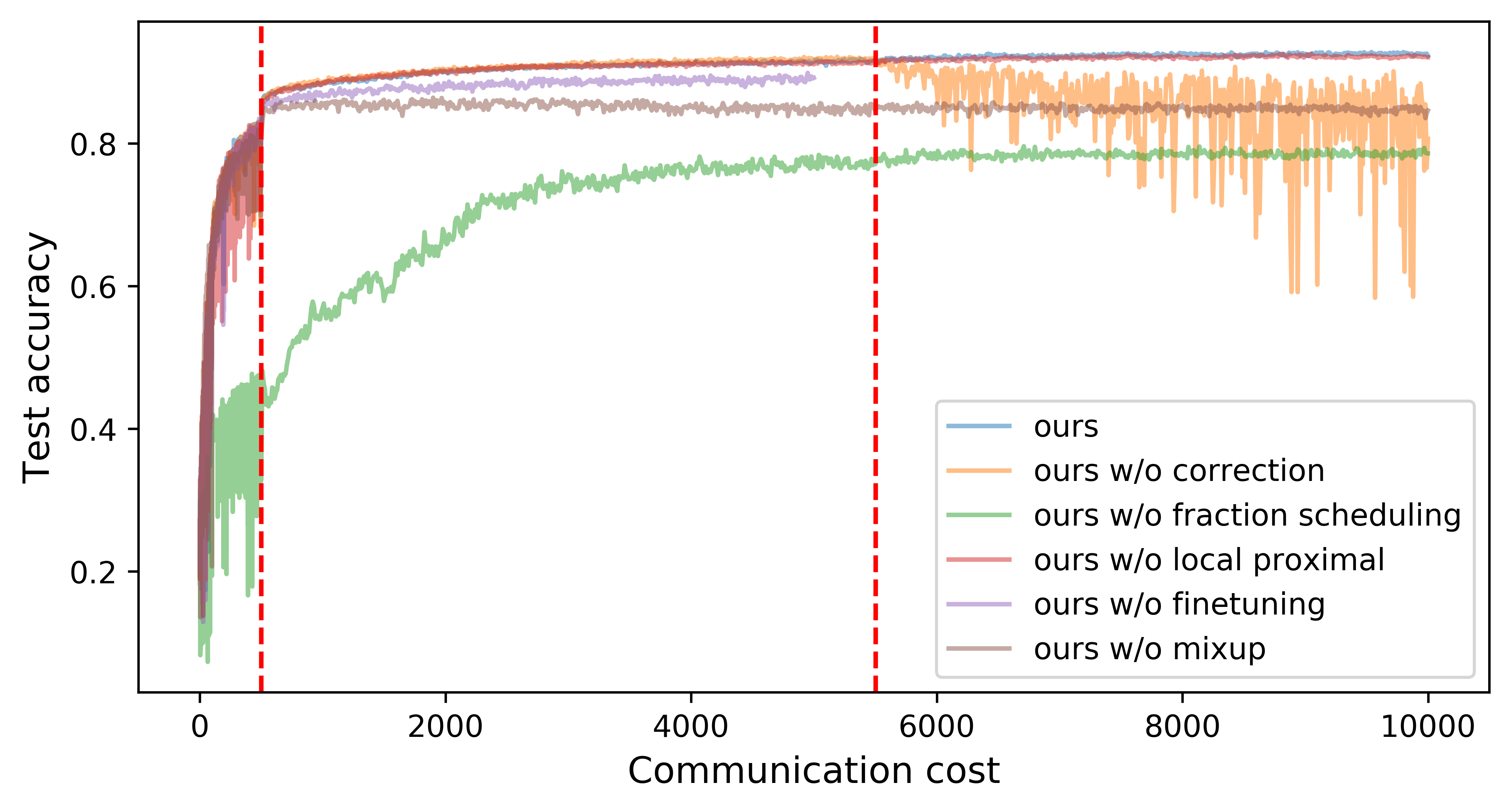
Figure 9: Ablation study results on the test accuracies of FedCorr during the training process, with each component removed. The experiments are evaluated on CIFAR-10 with IID data partition and noise setting $(\rho,\tau)=(0.6,0.5)$. The dotted lines represent the separation of the training process into our three stages.

C.6 Additional ablation study results

In Fig. 9, we show the effects of the components of FedCorr on test accuracies during training. In particular, note that without the finetuning stage, the total communication cost would be 5000. Hence in Fig. 9, the curve plotted for FedCorr without finetuning ends at the 5000 communication cost mark, which is to the left of the second red dotted line (5500 communication cost). As we mentioned in the main paper, fraction scheduling plays the most significant role in FedCorr. In addition, the label correction process would significantly improve training stability, especially in the usual training stage.

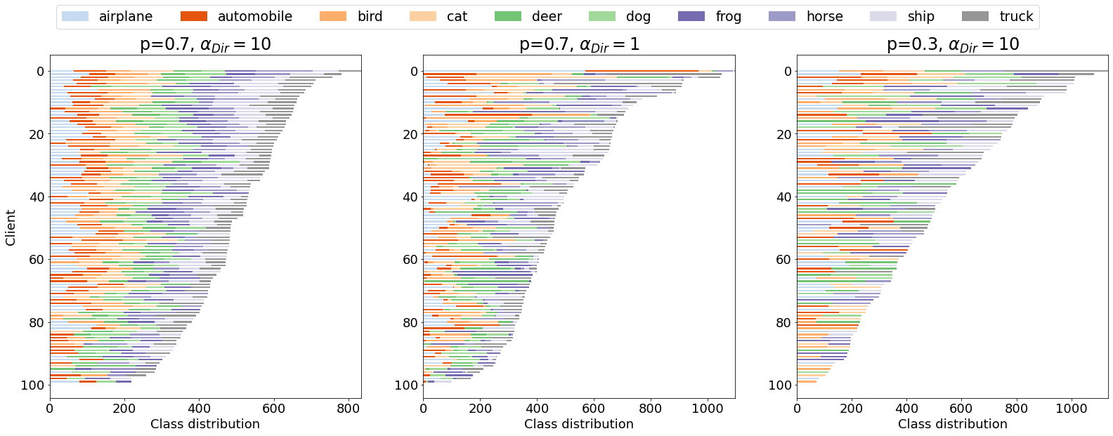
Figure 10: An illustration of three non-IID data partitions (via three different values for ($p$,$\alpha_{Dir}$)) on CIFAR-10, as used for our experiments reported in the main paper. For ease of viewing, we have sorted the clients according to their local dataset sizes in each of the three non-IID data partitions depicted. It should be noted that in our experiments, clients are not sorted; instead, clients are assigned data samples according to the data partition described in the main paper, which is a random process with no sorting.

C.7 Illustration of non-IID data partitions on CIFAR-10

As reported in the main paper, we used 3 different non-IID local data settings ($(p,\alpha_{Dir})=(0.7,10),(0.7,1),(0.3,10)$) for our experiment involving non-IID data partitions. In Fig. 10, we illustrate the detailed local class distributions and local dataset sizes for these three non-IID data settings on CIFAR-10, over $100$ clients.

Appendix D Potential negative impact: the issue of freeloaders

In real-world FL implementations, there is the implicit assumption that clients are collaborative and jointly collaborate to train a global model. Although FedCorr allows for a robust training of a global model even when some clients have label noise, this also includes the case when a client is a “freeloader”, where the client’s local dataset has completely random label noise (e.g. randomly assigning labels to an unlabeled dataset, without any actual non-trivial annotation effort). By participating in the FedCorr FL framework, such a “freeloader” would effectively use FedCorr as the actual annotation process, whereby identified noisy labels are corrected. Hence, this would be unfair to clients that have performed annotation on their local datasets prior to participating in FedCorr.

References

- [1] Durmus Alp Emre Acar, Yue Zhao, Ramon Matas, Matthew Mattina, Paul Whatmough, and Venkatesh Saligrama. Federated learning based on dynamic regularization. In International Conference on Learning Representations, 2020.
- [2] Laurent Amsaleg, Oussama Chelly, Teddy Furon, Stéphane Girard, Michael E Houle, Ken-ichi Kawarabayashi, and Michael Nett. Estimating local intrinsic dimensionality. In Proceedings of the 21th ACM SIGKDD International Conference on Knowledge Discovery and Data Mining, pages 29–38, 2015.
- [3] Eric Arazo, Diego Ortego, Paul Albert, Noel O’Connor, and Kevin McGuinness. Unsupervised label noise modeling and loss correction. In International Conference on Machine Learning, pages 312–321. PMLR, 2019.
- [4] Yiqiang Chen, Xiaodong Yang, Xin Qin, Han Yu, Biao Chen, and Zhiqi Shen. Focus: Dealing with label quality disparity in federated learning. In International Workshop on Federated Learning for User Privacy and Data Confidentiality in Conjunction with IJCAI(FL-IJCAI’20), 2020.
- [5] Zihan Chen, Kai Fong Ernest Chong, and Tony QS Quek. Dynamic attention-based communication-efficient federated learning. In International Workshop on Federated and Transfer Learning for Data Sparsity and Confidentiality in Conjunction with IJCAI (FTL-IJCAI’2021), 2021.
- [6] Yae Jee Cho, Jianyu Wang, and Gauri Joshi. Client selection in federated learning: Convergence analysis and power-of-choice selection strategies. arXiv preprint arXiv:2010.01243, 2020.
- [7] Shuhao Fu, Chulin Xie, Bo Li, and Qifeng Chen. Attack-resistant federated learning with residual-based reweighting. In AAAI Workshop Towards Robust, Secure and Efficient Machine Learning, 2021.
- [8] Bo Han, Quanming Yao, Tongliang Liu, Gang Niu, Ivor W Tsang, James T Kwok, and Masashi Sugiyama. A survey of label-noise representation learning: Past, present and future. arXiv preprint arXiv:2011.04406, 2020.
- [9] Bo Han, Quanming Yao, Xingrui Yu, Gang Niu, Miao Xu, Weihua Hu, Ivor W Tsang, and Masashi Sugiyama. Co-teaching: Robust training of deep neural networks with extremely noisy labels. In NeurIPS, 2018.
- [10] Kaiming He, Xiangyu Zhang, Shaoqing Ren, and Jian Sun. Deep residual learning for image recognition. In Proceedings of the IEEE conference on computer vision and pattern recognition, pages 770–778, 2016.
- [11] Michael E Houle. Dimensionality, discriminability, density and distance distributions. In 2013 IEEE 13th International Conference on Data Mining Workshops, pages 468–473. IEEE, 2013.
- [12] Michael E Houle. Local intrinsic dimensionality i: an extreme-value-theoretic foundation for similarity applications. In International Conference on Similarity Search and Applications, pages 64–79. Springer, 2017.
- [13] Tzu-Ming Harry Hsu, Hang Qi, and Matthew Brown. Measuring the effects of non-identical data distribution for federated visual classification. arXiv preprint arXiv:1909.06335, 2019.
- [14] Sohei Itahara, Takayuki Nishio, Yusuke Koda, Masahiro Morikura, and Koji Yamamoto. Distillation-based semi-supervised federated learning for communication-efficient collaborative training with non-iid private data. IEEE Transactions on Mobile Computing, 2021.
- [15] Sai Praneeth Karimireddy, Satyen Kale, Mehryar Mohri, Sashank Reddi, Sebastian Stich, and Ananda Theertha Suresh. Scaffold: Stochastic controlled averaging for federated learning. In International Conference on Machine Learning, pages 5132–5143. PMLR, 2020.
- [16] Alex Krizhevsky, Geoffrey Hinton, et al. Learning multiple layers of features from tiny images. 2009.
- [17] Yann LeCun, Bernhard Boser, John S Denker, Donnie Henderson, Richard E Howard, Wayne Hubbard, and Lawrence D Jackel. Backpropagation applied to handwritten zip code recognition. Neural computation, 1(4):541–551, 1989.
- [18] Junnan Li, Richard Socher, and Steven C.H. Hoi. Dividemix: Learning with noisy labels as semi-supervised learning. In International Conference on Learning Representations, 2020.
- [19] Tian Li, Shengyuan Hu, Ahmad Beirami, and Virginia Smith. Ditto: Fair and robust federated learning through personalization. In International Conference on Machine Learning, pages 6357–6368. PMLR, 2021.
- [20] Tian Li, Anit Kumar Sahu, Ameet Talwalkar, and Virginia Smith. Federated learning: Challenges, methods, and future directions. IEEE Signal Processing Magazine, 37(3):50–60, 2020.
- [21] Tian Li, Anit Kumar Sahu, Manzil Zaheer, Maziar Sanjabi, Ameet Talwalkar, and Virginia Smith. Federated optimization in heterogeneous networks. In Proceedings of Machine Learning and Systems, volume 2, pages 429–450, 2020.
- [22] Xiang Li, Kaixuan Huang, Wenhao Yang, Shusen Wang, and Zhihua Zhang. On the convergence of fedavg on non-iid data. In International Conference on Learning Representations, 2019.
- [23] Xiang Li, Kaixuan Huang, Wenhao Yang, Shusen Wang, and Zhihua Zhang. On the convergence of fedavg on non-iid data. arXiv preprint arXiv:1907.02189, 2019.
- [24] Xingjun Ma, Bo Li, Yisen Wang, Sarah M Erfani, Sudanthi Wijewickrema, Grant Schoenebeck, Dawn Song, Michael E Houle, and James Bailey. Characterizing adversarial subspaces using local intrinsic dimensionality. In International Conference on Learning Representations, 2018.
- [25] Xingjun Ma, Yisen Wang, Michael E Houle, Shuo Zhou, Sarah Erfani, Shutao Xia, Sudanthi Wijewickrema, and James Bailey. Dimensionality-driven learning with noisy labels. In International Conference on Machine Learning, pages 3355–3364. PMLR, 2018.
- [26] Brendan McMahan, Eider Moore, Daniel Ramage, Seth Hampson, and Blaise Aguera y Arcas. Communication-efficient learning of deep networks from decentralized data. In Artificial intelligence and statistics, pages 1273–1282. PMLR, 2017.
- [27] Sashank J. Reddi, Zachary Charles, Manzil Zaheer, Zachary Garrett, Keith Rush, Jakub Konečný, Sanjiv Kumar, and Hugh Brendan McMahan. Adaptive federated optimization. In International Conference on Learning Representations, 2021.
- [28] Karen Simonyan and Andrew Zisserman. Very deep convolutional networks for large-scale image recognition. In Yoshua Bengio and Yann LeCun, editors, 3rd International Conference on Learning Representations, ICLR 2015, San Diego, CA, USA, May 7-9, 2015, Conference Track Proceedings, 2015.
- [29] Sebastian U Stich. Local sgd converges fast and communicates little. arXiv preprint arXiv:1805.09767, 2018.
- [30] Daiki Tanaka, Daiki Ikami, Toshihiko Yamasaki, and Kiyoharu Aizawa. Joint optimization framework for learning with noisy labels. In Proceedings of the IEEE Conference on Computer Vision and Pattern Recognition, pages 5552–5560, 2018.
- [31] Ching Pui Wan and Qifeng Chen. Robust federated learning with attack-adaptive aggregation. In International Workshop on Federated and Transfer Learning for Data Sparsity and Confidentiality in Conjunction with IJCAI (FTL-IJCAI’2021), 2021.
- [32] Jianyu Wang, Qinghua Liu, Hao Liang, Gauri Joshi, and H Vincent Poor. Tackling the objective inconsistency problem in heterogeneous federated optimization. Advances in neural information processing systems, 2020.
- [33] Xiaobo Xia, Tongliang Liu, Bo Han, Nannan Wang, Mingming Gong, Haifeng Liu, Gang Niu, Dacheng Tao, and Masashi Sugiyama. Part-dependent label noise: Towards instance-dependent label noise. NeurIPS, 33, 2020.
- [34] Tong Xiao, Tian Xia, Yi Yang, Chang Huang, and Xiaogang Wang. Learning from massive noisy labeled data for image classification. In Proceedings of the IEEE conference on computer vision and pattern recognition, pages 2691–2699, 2015.
- [35] Jingyi Xu, Tony QS Quek, and Kai Fong Ernest Chong. Training classifiers that are universally robust to all label noise levels. In 2021 International Joint Conference on Neural Networks (IJCNN), pages 1–8. IEEE, 2021.
- [36] Xinyi Xu and Lingjuan Lyu. A reputation mechanism is all you need: Collaborative fairness and adversarial robustness in federated learning. In International Workshop on Federated Learning for User Privacy and Data Confidentiality in Conjunction with ICML(FL-ICML’21), 2021.
- [37] Qiang Yang, Yang Liu, Tianjian Chen, and Yongxin Tong. Federated machine learning: Concept and applications. ACM Transactions on Intelligent Systems and Technology (TIST), 10(2):1–19, 2019.
- [38] Seunghan Yang, Hyoungseob Park, Junyoung Byun, and Changick Kim. Robust federated learning with noisy labels. IEEE Intelligent Systems, 2022.
- [39] Dong Yin, Yudong Chen, Ramchandran Kannan, and Peter Bartlett. Byzantine-robust distributed learning: Towards optimal statistical rates. In Jennifer Dy and Andreas Krause, editors, Proceedings of the 35th International Conference on Machine Learning, volume 80 of Proceedings of Machine Learning Research, pages 5650–5659. PMLR, 10–15 Jul 2018.
- [40] Xingrui Yu, Bo Han, Jiangchao Yao, Gang Niu, Ivor Tsang, and Masashi Sugiyama. How does disagreement help generalization against label corruption? In ICML, pages 7164–7173. PMLR, 2019.
- [41] Hongyi Zhang, Moustapha Cisse, Yann N. Dauphin, and David Lopez-Paz. mixup: Beyond empirical risk minimization. In International Conference on Learning Representations, 2018.