Numerical ranges of Foguel operators revisited.

Abstract

The Foguel operator is defined as $F_{T}=\begin{bmatrix}S^{*}&T\\ 0&S\end{bmatrix}$, where $S$ is the right shift on a Hilbert space $\mathcal{H}$ and $T$ can be an arbitrary bounded linear operator acting on $\mathcal{H}$. Obviously, the numerical range $W(F_{0})$ of $F_{T}$ with $T=0$ is the open unit disk, and it was suggested by Gau, Wang and Wu in their LAA’2021 paper that $W(F_{aI})$ for non-zero $a\in\mathbb{C}$ might be an elliptical disk. In this paper, we described $W(F_{aI})$ explicitly and, as it happens, it is not.

1 Introduction and the main result

Let $\mathcal{H}$ be a Hilbert space. Denoting by $\langle.,.\rangle$ the scalar product on $\mathcal{H}$ and by $\left\|.\right\|$ the norm associated with it, recall that the numerical range of a bounded linear operator $A$ acting on $\mathcal{H}$ is the set

$$W(A):=\{\langle Ax,x\rangle\colon x\in\mathcal{H},\left\|x\right\|=1\}.$$

Clearly, $W(A)$ is a bounded subset of the complex plane $\mathbb{C}$; the numerical radius $w(A)$ defined as

$$w(A)=\sup\{\left|z\right|\colon z\in W(A)\}$$

does not exceed $\left\|A\right\|$ due to the Cauchy-Schwarz inequality. Furthermore, according to the celebrated Toeplitz-Hausdorff theorem, this set is also convex. The point spectrum (= the set of the eigenvalues) $\sigma_{p}(A)$ is contained in $W(A)$, while the whole spectrum $\sigma(A)$ is contained in its closure. A detailed up-to-date treatment of the numerical range properties and the history of the subject can be found in a recent comprehensive monograph [4].

In this paper, we consider Foguel operators, i.e., operators acting on $\mathcal{H}\oplus\mathcal{H}$ according to the block matrix representation

$$\quad F_{T}=\begin{bmatrix}S^{*}&T\\ 0&S\end{bmatrix}.$$ (1)

Here $S$ is the right shift while $T$ is an arbitrary operator on $\mathcal{H}$. Since $W(S)=W(S^{*})$ coincides with the open unit disk $\mathbb{D}$, for any $T$ we have

$$\quad W(F_{T})\supseteq\mathbb{D}.$$ (2)

In particular, $w(F_{T})\geq 1$.

In [2] some more specific estimates for $w(F_{T})$ were established for an arbitrary $T$, while for $T=aI$ the exact formula $w(F_{aI})=1+\left|a\right|/2$ was obtained. In the latter case it was also proved in [2] that $W(F_{aI})$ is open, and conjectured that it is an elliptical disk with the minor half-axis $\sqrt{1+\left|a\right|^{2}/4}$. (The case $a=0$ is of course obvious, since $F_{0}=S^{*}\oplus S$ and so $W(F_{0})=\mathbb{D}$.)

As we will show, this conjecture does not hold. The numerical range of $F_{aI}$ can be described explicitly, and this description is as follows.

Theorem 1.

Let $A$ be given by (1) with $T=aI$. Then the numerical range of $A$ is symmetric with respect to both coordinate axes, bounded on the right/left by arcs of the circles centered at $(\pm 1,0)$ and having radius $r=\left|a\right|/2$, and from above/below by arcs of the algebraic curve defined by the equation

$$\quad\begin{gathered}16r^{6}(u+v)^{2}-8r^{4}\left(u^{3}+(v-1)(4u^{2}+5uv-u+2v^{2})-v\right)\\ +r^{2}\left(((u-20)u-8)v^{2}+2((u-15)u-4)(u-1)v\right.\\ \left.+((u-10)u+1)(u-1)^{2}\right)+(u-1)^{3}(u+v-1)=0\end{gathered}$$ (3)

in terms of $u=x^{2},\ v=y^{2}$. The switching points between the arcs are located on the supporting lines of $W(A)$ forming the angles $\pm\cos^{-1}\frac{\sqrt{4+r^{2}}-r}{2}$ with the $y$-axis.

The proof of Theorem 1 is split between the next two sections. In Section 2, the parametric description of the supporting lines to $W(F_{aI})$ is derived. Section 3 is devoted to the transition from that to the point equation of $\partial W(F_{aI})$. Note that the formulas in Section 2 are obtained via a somewhat unexpected application of Toeplitz operators technique.

2 $W(F_{aI})$ in terms of its supporting lines

As any convex subset of $\mathbb{C}$, the numerical range of a bounded linear operator $A$ is completely determined by the family of its supporting lines. The latter has the form

$$\quad\omega\left(\lambda_{\max}(\operatorname{Re}(\overline{\omega}A))+i\mathbb{R}\right),\quad\omega=e^{i\theta}\text{ with }\theta\in[-\pi,\pi].$$ (4)

(We are using the standard notation $\operatorname{Re}X:=(X+X^{*})/2$ for the hermitian part of an operator $X$, and $\lambda_{\max}(H)$ for the rightmost point of $\sigma(H)$ when $H$ is a hermitian operator.)

For $A=F_{T}$ given by (1) we are therefore interested in the non-invertibility of the operator

$$\quad\begin{bmatrix}X_{\omega}-2\lambda I&\overline{\omega}T\\ \omega T^{*}&X_{\overline{\omega}}-2\lambda I\end{bmatrix},$$ (5)

where

$$\quad X_{\omega}:=\omega S+\overline{\omega}S^{*}.$$ (6)

Due to (2), we know a priori that the values of $\lambda_{\max}$ in (4) are all greater than or equal to one. So, we may suppose that in (5) $\lambda>1$.

Under this condition, the diagonal blocks of (5) are invertible and, according to the Schur complement the operator (5) is (or is not) invertible simultaneously with $X_{\overline{\omega}}-2\lambda I-T^{*}(X_{\omega}-2\lambda I)^{-1}T$. For $T=aI$ this expression simplifies further to

$$\quad X_{\overline{\omega}}-2\lambda I-\left|a\right|^{2}(X_{\omega}-2\lambda I)^{-1}.$$ (7)

Replacing $\left|a\right|/2$ by $r$, as in the statement of the theorem, and multiplying (7) by $X_{\omega}-2\lambda I$, we see that for $\lambda>1$ the operator (5) is invertible only simultaneously with

$$\quad X_{\overline{\omega}}X_{\omega}-2\lambda(X_{\omega}+X_{\overline{\omega}})+4(\lambda^{2}-r^{2})I.$$ (8)

Lemma 1.

Let $\omega\neq\pm 1,\pm i$. Then the operator (8) is not invertible if and only if $2(r^{2}-\lambda^{2})$ lies in the range of the function

$$\quad f_{\lambda,\omega}(t)=\operatorname{Re}(t^{2})+\operatorname{Re}(\omega^{2})-4\lambda\operatorname{Re}t\operatorname{Re}\omega,\quad t\in\mathbb{T}.$$ (9)

Proof of this Lemma uses some notions concerning Hardy spaces and Toeplitz operators; interested readers are referred to excellent monographs available on the subject, e.g., [1] or [3].

Proof.

Let us consider the realization of $\mathcal{H}$ as the Hardy space $H^{2}$ of functions analytic on $\mathbb{D}$ with their Taylor coefficients forming an $\ell^{2}$ sequence. This space identifies naturally with a subspace of $L^{2}$ on the boundary of $\mathbb{D}$, the unit circle $\mathbb{T}$. Denote by $P$ the orthogonal projection of $L^{2}(\mathbb{T})$ onto $H^{2}$, and recall that for any $\phi\in L^{\infty}(\mathbb{T})$ the Toeplitz operator with the symbol $\phi$ is defined as

$$(T_{\phi}=:)\ P\phi P\colon H^{2}\longrightarrow H^{2}.$$

When $\phi\in H^{\infty}$ (the space of bounded analytic function on $\mathbb{D}$), $T_{\phi}$ is simply the multiplication by $\phi$. Such is, in particular, the shift operator $S$, which for $\mathcal{H}=H^{2}$ is nothing but the multiplication by the variable $z$:

$$(Sf)(z)=zf(z),\quad f\in H^{2}.$$

Accordingly, the operator $X_{\omega}$ defined by (6) is the Toeplitz operator with the symbol $\omega t+\overline{\omega}t^{-1}$, and (8) takes the form

$$P(\overline{\omega}t+\omega t^{-1})P(\omega t+\overline{\omega}t^{-1})P-2\lambda P(\omega t+\overline{\omega}t^{-1}+\overline{\omega}t+\omega t^{-1})P+4(\lambda^{2}-r^{2})I.$$

Replacing the middle $P$ in the first term by $I-Q$, where $Q$ is the projection of $L^{2}(\mathbb{T})$ onto the orthogonal complement of $H^{2}$, we can further rewrite (8) as $2T_{f}-\overline{\omega}^{2}P_{0}+4(\lambda^{2}-r^{2})I$. Here $f=f_{\lambda,\omega}$ is given by (9), and $P_{0}=P(t+\omega^{2}t^{-1})Q(\omega^{2}t+t^{-1})P$. Considering that $Pt^{-1}Q=QtP=0$, $P_{0}$ simplifies to $PtQt^{-1}P$, which is nothing but the rank one orthogonal projection mapping each $f\in H^{2}$ to its constant term. So, the operator (8) is not invertible if and only if

$$\quad 2(r^{2}-\lambda^{2})\in\sigma\left(T_{f}-\frac{\overline{\omega}^{2}}{2}P_{0}\right).$$ (10)

Observe that the essential spectrum of the operator $T_{f}-\frac{\overline{\omega}^{2}}{2}P_{0}$ is the same as that of the Toeplitz operator $T_{f}$. Since the function $f$ is real-valued, the latter coincides with $\sigma(T_{f})$. So, the right hand side of (10) is $\sigma(T_{f})$ possibly united with some isolated eigenvalues of $T_{f}-\frac{\overline{\omega}^{2}}{2}P_{0}$.

Our next step is to observe that for non-real $\omega^{2}$ such eigenvalues, if exist, cannot be real. Indeed, denoting by $\xi$ the respective eigenfunction and writing $T_{f}-\frac{\overline{\omega}^{2}}{2}P_{0}$ as $H+iK$ with $H,K$ hermitian, we would then have $\langle K\xi,\xi\rangle=0$. But $K=\frac{\operatorname{Im}(\omega^{2})}{2}P_{0}$, and so $\langle K\xi,\xi\rangle$ is a non-zero multiple of $\left|\xi(0)\right|^{2}$. From here, $P_{0}\xi=\xi(0)=0$, and $\xi$ is an eigenfunction of $T_{f}$ corresponding to the same eigenvalue $\mu$. This is a contradiction.

So, for $\omega\neq\pm 1,\pm i$ condition (10) is equivalent to $2(r^{2}-\lambda^{2})\in\sigma(T_{f})$. It remains to invoke the fact that, since the function $f$ is continuous, $\sigma(T_{f})$ equals the range of $f$. ∎

Recall that we are interested in the maximal values of $\lambda$ satisfying the conditions of Lemma 1. The explicit formulas for them are provided in the following statement.

Lemma 2.

Let $f$ be defined by (9). Then the maximal value of $\lambda$ satisfying

$$\quad 2(r^{2}-\lambda^{2})\in f(\mathbb{T})$$ (11)

is

$$\quad\lambda_{\max}(\theta)=\begin{cases}r+\left|\operatorname{Re}\omega\right|&\text{ if }\left|\operatorname{Re}\omega\right|\geq(\sqrt{4+r^{2}}-r)/2,\\ \sqrt{1+(r/\operatorname{Im}\omega)^{2}}&{\text{o}therwise.}\end{cases}$$ (12)

Proof.

Formulas (12) are invariant under substitutions $\omega\mapsto-\omega$ and $\omega\mapsto\overline{\omega}$. Since also $f_{\lambda,\omega}=f_{\lambda,\overline{\omega}}$ and $f_{\lambda,\omega}(t)=f_{\lambda,-\omega}(-t)$, it suffices to consider $\omega$ lying in the first quadrant only. So, in what follows $\omega=e^{i\theta}$ with $\cos\theta,\sin\theta\geq 0$.

A straightforward calculus application yields

$$f(\mathbb{T})=\begin{cases}[2\cos^{2}\theta-4\lambda\cos\theta,2\cos^{2}\theta+4\lambda\cos\theta]&\text{ if }\lambda\cos\theta\geq 1,\\ [2(1-\lambda^{2})\cos^{2}\theta-2,2\cos^{2}\theta+4\lambda\cos\theta]&\text{ otherwise}.\end{cases}$$

After some simplifications, (11) can therefore be rewritten as

$$r\in[\lambda-\cos\theta,\lambda+\cos\theta],\quad\lambda\cos\theta\geq 1,$$

or

$$r\in[\sqrt{\lambda^{2}-1}\sin\theta,\lambda+\cos\theta],\quad\lambda\cos\theta\leq 1.$$

In terms of $\lambda$, these conditions are equivalent to $\lambda\in\Lambda_{1}\cup\Lambda_{2}$, where

$$\Lambda_{1}=\left[\max\{r-\cos\theta,\sec\theta\},r+\cos\theta\right]$$

and

$$\Lambda_{2}=\left[r-\cos\theta,\min\{\sqrt{1+(r/\sin\theta)^{2}},\sec\theta\}\right],$$

respectively.

The remaining reasoning depends on the relation between $\sec\theta-\cos\theta$ and $r$ (equivalently, between $\cos\theta$ and $(\sqrt{4+r^{2}}-r)/2$).

Case 1. $r\geq\sec\theta-\cos\theta$. Then $\max\Lambda_{1}=r+\cos\theta\geq\sec\theta\geq\max\Lambda_{2}$.

Case 2. $r<\sec\theta-\cos\theta$. This inequality implies $\sqrt{1+(r/\sin\theta)^{2}}<\sec\theta$, and so $\max\Lambda_{2}=\sqrt{1+(r/\sin\theta)^{2}}$ while $\Lambda_{1}=\emptyset$.

These findings agree with (12) thus completing the proof. ∎

So, at least for $\omega\neq\pm 1,\pm i$, the supporting lines of $W({F_{aI}})$ are given by

$$\quad\omega\left(\lambda_{\max}(\theta)+i\mathbb{R}\right),\quad\omega=e^{i\theta}\text{ with }\theta\in[-\pi,\pi]$$ (13)

and $\lambda_{\max}(\theta)$ as in (12). Due to the continuity of $\lambda_{\max}$ at the a priori excluded values of $\omega$, this description actually holds throughout.

To illustrate, below is the plot of the supporting lines of $W(F_{aI})$ corresponding to $a=1$.

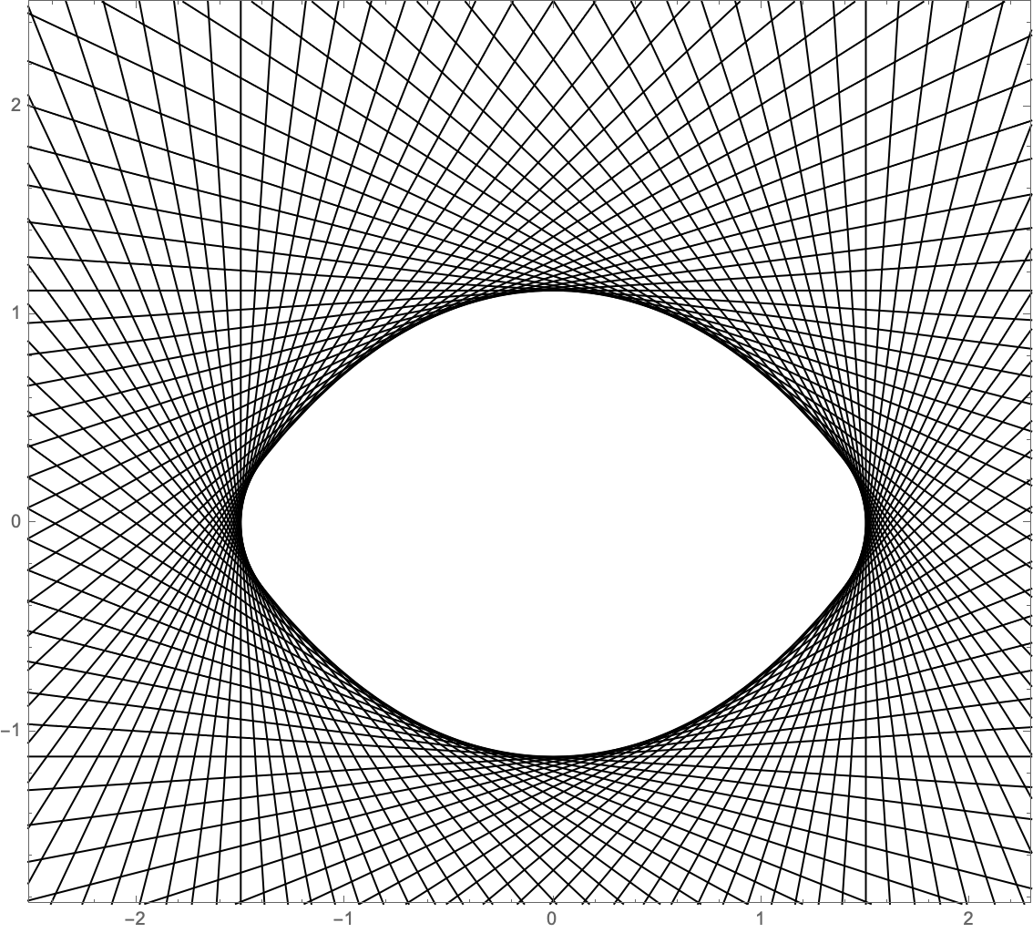
Figure 1: Supporting lines of $W(F_{I})$.

3 From supporting lines to the point description

With formulas (12) describing the supporting lines, we can derive the point equation for the envelope curve explicitly. The respective standard procedure is to exclude $\theta$ from the system of equations

$$\quad f(x,y,\theta)=0,\quad f^{\prime}_{\theta}(x,y,\theta)=0,$$ (14)

where the former represents the family of lines (13) in a parametric form. In accordance with (12), there are two cases to consider, depending on the relation between $\left|\cos\theta\right|$ and the value of $(\sqrt{4+r^{2}}-r)/2$.

Proposition 2.

Let $\left|\cos\theta\right|>(\sqrt{4+r^{2}}-r)/2$. The respective portion of the envelope of (13) consists of arcs of the circles of radius $r$ centered at $\pm 1$.

Proof.

Plugging $\lambda_{\max}(\theta)$ from the upper line of (12) into (13) yields

$$f(x,y,\theta)=(x\mp 1)\cos\theta+y\sin\theta-r.$$

From here,

$$f^{\prime}_{\theta}=-(x\mp 1)\sin\theta+y\cos\theta,$$

and solving the respective system (14) yields $x\mp 1=r\cos\theta,y=r\sin\theta$. ∎

The remaining case is more involved.

Proposition 3.

Let $\left|\cos\theta\right|<(\sqrt{4+r^{2}}-r)/2$. The respective portion of the envelope of (13) lies on the algebraic curve defined by (3).

Proof.

With $\lambda_{\max}$ given by the second line in (12), the system (14) (at least, in the first quadrant — which is sufficient for our purposes) takes the form

$$\begin{cases}x\cos\theta+y\sin\theta=\sqrt{(r/\sin\theta)^{2}+1}/2,\\ x\sin\theta-y\cos\theta=\frac{r^{2}\cos\theta}{2\sin^{3}\theta\sqrt{(r/\sin\theta)^{2}+1}}.\end{cases}$$

Replacing this system by the square of its first equation and its product with the second yields

$$\begin{cases}(x\cos\theta+y\sin\theta)^{2}=\left((r/\sin\theta)^{2}+1\right)/4,\\ (x\sin\theta-y\cos\theta)(x\cos\theta+y\sin\theta)=r^{2}\cos\theta/\sin^{3}\theta.\end{cases}$$

Using the universal trigonometric substitution $t=\tan(\theta/2)$ turns the latter system into

$$\quad\begin{cases}&-r^{2}t^{10}-3r^{2}t^{8}-2t^{6}\left(r^{2}-8x^{2}+8y^{2}\right)+2t^{4}\left(r^{2}-8x^{2}+8y^{2}\right)\\ &+3r^{2}t^{2}+r^{2}+8t^{7}xy-48t^{5}xy+8t^{3}xy=0,\\ &-r^{2}t^{8}-4t^{6}\left(r^{2}-x^{2}+1\right)-2t^{4}\left(3r^{2}+4x^{2}-8y^{2}+4\right)\\ &-4t^{2}\left(r^{2}-x^{2}+1\right)-r^{2}-16t^{5}xy+16t^{3}xy=0.\end{cases}$$ (15)

Equation (3) is nothing but the resultant of (15) considered as the system of two polynomials in $t$, obtained with the aid of Mathematica. ∎

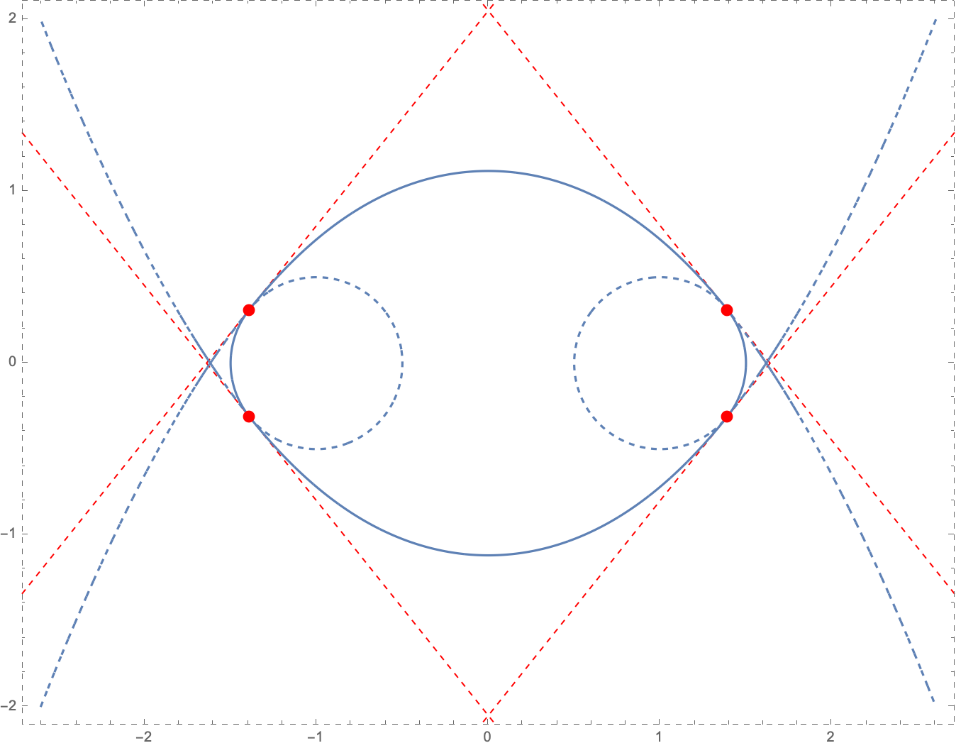
Figure 2: Boundary of $W(F_{I})$ (solid blue curve).

In Fig. 2, the circles and “parabola-like” curves containing the arcs of $\partial W(F_{I})$ are plotted as blue dashed lines; red dashed lines are the supporting lines of $W(F_{I})$ at the switching points (red dots) between the two types of boundary arcs.

References

- [1] A. Böttcher and B. Silbermann, Analysis of Toeplitz operators, second ed., Springer Monographs in Mathematics, Springer-Verlag, Berlin, 2006, Prepared jointly with A. Karlovich.
- [2] H.-L. Gau, K.-Z. Wang, and P. Y. Wu, Numerical ranges of Foguel operators, Linear Algebra Appl. 610 (2021), 766–784.
- [3] N. Nikolski, Hardy spaces, French ed., Cambridge Studies in Advanced Mathematics, vol. 179, Cambridge University Press, Cambridge, 2019.
- [4] P. Y. Wu and H.-L. Gau, Numerical ranges of Hilbert space operators, Encyclopedia of Mathematics and its Applications, vol. 179, Cambridge University Press, Cambridge, 2021.