Quasistatic Evolution with Unstable Forces

Abstract

We consider load controlled quasistatic evolution. Well posedness results for the nonlocal continuum model related to peridynamics are established. We show local existence and uniqueness of quasistatic evolution for load paths originating at stable critical points. These points can be associated with local energy minima among the convex set of deformations belonging to the strength domain of the material. The evolution of the displacements however is not constrained to lie inside the strength domain of the material. The load-controlled evolution is shown to exhibit energy balance.

74A70, 74A20, 74A45

1 Introduction

The model studied here is a nonlocal continuum model where the length scale of force interaction between points is taken to be at least an order of magnitude smaller than the characteristic length of the domain. We pose a nonlinear and nonlocal field theory of peridynamic (PD) type [SILLING2000175]. The unknown is the displacement field $\mathbf{u}$ at a point $\mathbf{x}$ in the body at time $t$. For PD models the force interaction occurs between a point $\mathbf{x}$ and another point $\mathbf{y}$ when $\mathbf{y}$ lies within a sphere $H_{\epsilon}(\mathbf{x})$ of radius $\epsilon$ centered at $\mathbf{x}$. The force between $\mathbf{x}$ and $\mathbf{y}$, is determined by the displacement at each point through a constitutive law. The net force on $\mathbf{x}$ is the force averaged over all $\mathbf{y}$ in the sphere. The radius $\epsilon$ is often referred to as the horizon. The net force is referred to as the PD force of the body acting on $\mathbf{x}$. The constitutive law used here is of cohesive type; the force between two points initially increases with strain until a maximum force is reached and then the force decreases to zero with a continued increase in strain.

The objective of PD field theory is to account for elastic interaction where the material is intact as well as the emergence and propagation of failure zones characterized by vanishing force. PD models are inherently multiscale, coupling fracture caused by breaking bonds at the atomic scale with elastic deformation at the macroscopic scale. Dynamic simulations for cohesive PD show that failure zones are naturally localized by the model and appear as thin and crack like [lipton2019complex, jhalipton2020]. Both localization and emergent behavior is the hallmark of simulations using the PD formulation introduced in [SILLING2000175, silling2007peridynamic], see for example [silling2005meshfree, bobaru2010peridynamic, oterkus2014fully, Kilic2009, silling2017modeling, madenci2017ordinary, parksyueyoutrask] where different PD models are developed and applied. There is a growing mathematical theory supporting well posedness of the nonlocal fracture modeling and numerical simulations for different PD fracture models [emmrichpuhst2016, dutian2018, lipton2018free, jha2018numerical, parksyueyoutrask]. Cohesive PD models like the one considered here are seen to recover classic Griffith fracture energy from the PD energy in the limit $\epsilon\rightarrow 0$ through $\Gamma$ convergence, [lipton2014horizonlimit, lipton2016cohesive, lipton2019complex]. Convergence of PD fields adjacent to crack like defects to elastic fields with zero normal traction on classic cracks as well as the classic kinetic relations for crack growth (see [Freund, ravi2004dynamic, anderson2017fracture]) are recovered in the $\epsilon=0$ limit [liptonjha2021, jhalipton2020].

In the absence of inertia one considers quasistatic or rate independent evolution. Nonlocal formulations of rate independent linearized plastic evolution is formulated and solved [kruvzik2018quasistatic]. There it is shown that the nonlocal peridynamic model $\Gamma$ converges to classic local elastoplasticity as the interaction range goes to zero. Nonlocal equilibrium problems for linear elasticity are shown to $\Gamma$ converge to classic elastic boundary value problems [mengesha2015variational]. Nonlocal multiscale peridynamic models have been shown to rigorously to recover classic strongly coupled local theories of elasticity with highly oscillatory coefficients [scott2020asymptotic]. Memory effects are recovered by two scale limits of highly oscillatory linear nonlocal models using two-scale homogenization [alali2012multiscale, du2016multiscale].

This article investigates the quasi-static regime using the constitutive model of cohesive PD. We consider the zero inertia limit and focus on the rate independent evolution governed by the PD equations in the absence of acceleration. The approach to evolution taken here is a departure from the quasistatic evolution of global energy mininimizers. Given a body $\Omega\in\mathbb{R}^{d}$, $d=2,\,3$ we assume at $t=0$ and for $\mathbf{x}\in\Omega$ that there exists a displacement $\mathbf{u}_{0}=\mathbf{u}(\mathbf{x},0)$ and body force $\mathbf{b}(\mathbf{x},0)$ for which we have force balance

(1) $$\mathcal{L}[\mathbf{u}_{0}](\mathbf{x})=\mathbf{b}(\mathbf{x},0),$$

where $\mathcal{L}[\mathbf{u}_{0}](\mathbf{x})$ is the force at $\mathbf{x}$ due to the deformation $\mathbf{u}_{0}$ and given by (8). The quasistatic evolution $\mathbf{u}(t)=\mathbf{u}(\mathbf{x},t):t\in[0,T]$ is given by

(2) $$\mathcal{L}[\mathbf{u}(t)](\mathbf{x})=\mathbf{b}(\mathbf{x},t).$$

for a prescribed load path $\mathbf{b}(\mathbf{x},t):t\in[0,T]\to\mathbb{R}^{2}$. Here $t$ appears as a load parameter and the load path is independent of parameterization. We show existence of an evolution in a neighborhood of $(\mathbf{u}_{0},\mathbf{b}_{0})$ provided the inverse of the Fréchet derivative of $\mathcal{L}[\mathbf{u}(t)]$ exists at $\mathbf{u}_{0}$, see theorem 2. When the load $\mathbf{b}(t)$ is smooth and the Fréchet derivative of $\mathcal{L}[\mathbf{u}(t)]$ is invertible for $t\in[0,T]$ then the quasistatic evolution satisfies energy balance, see theorem 8 of section 3.

A displacement $\mathbf{u}(\mathbf{x},t)$ is said to be in the strength domain if its strain

$$S(\mathbf{y},\mathbf{x})=\frac{\mathbf{u}(\mathbf{y})-\mathbf{u}(\mathbf{x})}{|\mathbf{y}-\mathbf{x}|}\cdot\frac{\mathbf{y}-\mathbf{x}}{|\mathbf{y}-\mathbf{x}|},$$

increases with increasing force for every $\mathbf{y}$ in the neighborhood of every point in the body, see Definition 1. If there is a set of points for which force begins to decrease inside their neighborhoods then the deformation lies outside the strength domain. The collection of such points are called softening zones. The key feature is that the force $\mathcal{L}[\mathbf{u}(t)](\mathbf{x})$ remains defined for all points of the body. Here material damage is represented by the softening zone and its propagation is part of the quasistatic evolution.

Next we consider the case when $\mathbf{b}_{0}$ is such that the solution $\mathbf{u}_{0}$ of (1) lies inside the strength domain. For this case we introduce a stability tensor field defined at every point $\mathbf{x}$ in the body, see Definition 3 of section 3. We discover that the stability tensor is positive definite when the domain satisfies an interior cone condition and the deformation field lies inside the strength domain of the material, see theorem 4 of section 3. The interior cone condition automatically excludes sharp domains see figure 2. For this case we can show that the Fréchet derivative of $\mathcal{L}[\mathbf{u}_{0}]$ is invertible and conclude that a quasistatic evolution exists in an neighborhood of $(\mathbf{b}_{0},\mathbf{u}_{0}$), see the discussion below theorem 4.

We relate the existence of a local evolution to the existence of a local minimizer of a PD energy. We show that a quasi-static PD evolution exists within a neighborhood of a local energy minimizer. Here the minimizing displacement is a local minimizer among fields belonging to the strength domain of the material, see Theorem 6 of section 3. If instead the displacement $\mathbf{u}_{0}$ does not lie in the strength domain we present more general sufficient conditions for invertability given in Theorem LABEL:esistence_of_inverse_in_strength_domain. Part of the sufficient conditions require that all eigenvalues of $\mathbb{A}[\mathbf{u}]$ lie outside an open interval containing $0$. We present a necessary condition of invertability of the Fréchet derivative of $\mathcal{L}[\mathbf{u}_{0}]$ in terms of the stability tensor that shows that $\mathbb{A}[\mathbf{u}]$ can not have a zero eigenvalue on a subset of finite measure on $\Omega$, see Theorem 7 of section 3. The stability tensor is defined here for the quasistatic case but agrees in form with the stability tensor introduced for dynamic fracture in [sillingweknerascaribobaru] and in [lipton2014horizonlimit, lipton2019complex]. This tensor appears again for elasto-dynamic problems and in energy minimization for equilibrium problems in [DuGunLehZho, MengeshaDuNonlocal14] and elasto-static problems with sign changing kernel [MengeshaDu]. Much of the theory developed here provides the foundation for the quasistatic fracture theory developed and implemented in the sequel [BhattacharyaLiptonDiehl].

The PD model is described in section 2 and the main results are provided in section 3. The proofs of all theorems are provided in sections 4 through LABEL:sec:necessary. The article concludes with a summary of results.

2 Background and problem formulation

In this paper both two and three dimensional nonlocal formulations are considered. For dynamics the deformation field $\mathbf{u}(\mathbf{x},t)$ of a material point $\mathbf{x}$ in the domain $\Omega\subset\mathbb{R}^{d},\,\,d=2,3$, at time $t$ satisfies the momentum-balance equation

(3) $$\rho\ddot{\mathbf{u}}(\mathbf{x},t)=\int\limits_{H_{\epsilon}(\mathbf{x})\cap\Omega}\mathbf{f}(\mathbf{y},\mathbf{x},\mathbf{u},t)d\mathbf{y}+\mathbf{b}(\mathbf{x},t),\ \mathbf{x}\in\Omega$$

where $\rho$ is the material density, $H_{\epsilon}(\mathbf{x})$ is a sphere centered at the point $\mathbf{x}$ with radius $\epsilon$ and $\mathbf{b}$ is the body force density. Here, $H_{\epsilon}(\mathbf{x})\cap\Omega$ is the set of neighboring points $\mathbf{y}$ in $\Omega$ that can interact with $\mathbf{x}$. The parameter $\epsilon$ is called the horizon. The force interaction between $\mathbf{x}$ and $\mathbf{y}$ is mediated by $\mathbf{f}(\mathbf{y},\mathbf{x},\mathbf{u},t)$ that denotes the force density exerted by a point $\mathbf{y}\in H_{\epsilon}(\mathbf{x})$ on $\mathbf{x}$ and is taken to be a function of internal displacement at time $t$.

When the effect of inertia can be ignored (3) reduces to the quasi-static formulation given by

(4) $$\int\limits_{H_{\epsilon}(\mathbf{x})\cap\Omega}\mathbf{f}(\mathbf{y},\mathbf{x},\mathbf{u})d\mathbf{y}+\mathbf{b}(\mathbf{x},t)=0.$$

We introduce the nonlocal strain $S(\mathbf{y},\mathbf{x},\mathbf{u})$ between the point $\mathbf{x}$ and any point $\mathbf{y}\in H_{\epsilon}(\mathbf{x})$ given by

(5) $$S(\mathbf{y},\mathbf{x},\mathbf{u})=\frac{\mathbf{u}(\mathbf{y})-\mathbf{u}(\mathbf{x})}{\left\lvert\mathbf{y}-\mathbf{x}\right\rvert}\cdot\mathbf{e}_{\mathbf{y}-\mathbf{x}},$$

where $\mathbf{e}_{\mathbf{y}-\mathbf{x}}$ is the unit vector given by

$$\mathbf{e}_{\mathbf{y}-\mathbf{x}}=\frac{\mathbf{y}-\mathbf{x}}{\left\lvert\mathbf{y}-\mathbf{x}\right\rvert}.$$

Force is related to strain using the constitutive relation given by the cohesive force law [lipton2014horizonlimit, lipton2016cohesive]. Under this law the force is linear for small strains and for larger strains the force begins to soften and then approaches zero after reaching a critical strain. The nonlocal force density $\mathbf{f}$ is given in terms of the nonlocal potential $\mathcal{W}(S)$ by

(6) $$\mathbf{f}(\mathbf{y},\mathbf{x},\mathbf{u})=2\partial_{S}\mathcal{W}(S(\mathbf{y},\mathbf{x},\mathbf{u}))\mathbf{e}_{\mathbf{y}-\mathbf{x}},$$

where

(7) $$\mathcal{W}(S(\mathbf{y},\mathbf{x},\mathbf{u}))=\frac{J^{\epsilon}(\left\lvert\mathbf{y}-\mathbf{x}\right\rvert)}{\epsilon^{d+1}\omega_{d}\left\lvert\mathbf{y}-\mathbf{x}\right\rvert}g(\sqrt{\left\lvert\mathbf{y}-\mathbf{x}\right\rvert}S(\mathbf{y},\mathbf{x},\mathbf{u})).$$

Here, $J^{\epsilon}(r)=J(\frac{r}{\epsilon})$, where $J$ is a non-negative bounded function supported on $[0,1]$. $J$ is called the influence function as it determines the influence of the bond force of peridynamic neighbors $\mathbf{y}$ on the center $\mathbf{x}$ of $H_{\epsilon}(\mathbf{x})$. The volume of unit ball in $\mathbb{R}^{d}$ is denoted by $\omega_{d}$. As figure 1 illustrates we assume that $g(r)$ and the derivatives $g^{\prime}(r)$, $g^{\prime\prime}(r)$, and $g^{\prime\prime\prime}(r)$ are bounded for $-\infty<r<\infty$. It is required is that $g(0)=0$ and $g(r)>0$ otherwise, $g(r)$ together with its first three derivatives must be bounded, and that $g$ be convex in the interval $r^{e}<0<r^{c}$ and concave outside this interval with finite limits $\lim_{r\rightarrow-\infty}{g(r)}=C^{-}$ and $\lim_{r\rightarrow\infty}{g(r)}=C^{+}$. Additionally $\max\{|g^{\prime\prime}(r|)\}=g^{\prime\prime}(0)$. The quasistatic peridynamic equation (4) is expressed by

$$\mathcal{L}[\mathbf{u}](\mathbf{x},t)=\mathbf{b}(\mathbf{x},t),\ \mathbf{x}\in\Omega,$$

where the integral operator $\mathcal{L}$ is defined as

(8) $$\mathcal{L}[\mathbf{u}](\mathbf{x},t)=-\int\limits_{H_{\epsilon}(\mathbf{x})\cap\Omega}{2}\frac{J^{\epsilon}(\left\lvert\mathbf{y}-\mathbf{x}\right\rvert)}{\epsilon^{d+1}\omega_{d}\sqrt{\left\lvert\mathbf{y}-\mathbf{x}\right\rvert}}g^{\prime}\left(\sqrt{\left\lvert\mathbf{y}-\mathbf{x}\right\rvert}S(\mathbf{y},\mathbf{x},\mathbf{u})\right)\mathbf{e}_{\mathbf{y}-\mathbf{x}}d\mathbf{y}.$$

For this model the strength domain of the material is simple and can be described in terms of the strain $S(\mathbf{y},\mathbf{x},\mathbf{u})$.

Definition 1.

Strength Domain. For $\mathbf{x}\in\Omega$ and $\mathbf{y}\in\Omega\cap H_{\epsilon}(\mathbf{x})$ the strength domain of the material is given by all displacements with strain inside the interval

(9) $${r^{e}}<\sqrt{|\mathbf{y}-\mathbf{x}|}S(\mathbf{y},\mathbf{x},\mathbf{u})<r^{c},$$

or

(10) $$\frac{r^{e}}{\sqrt{|\mathbf{y}-\mathbf{x}|}}<S(\mathbf{y},\mathbf{x},\mathbf{u})<\frac{r^{c}}{\sqrt{|\mathbf{y}-\mathbf{x}|}}.$$

This is the set of strains where the magnitude of force increases with increasing strain. Material failure occurs for strains outside this interval where the force becomes unstable. Moreover $g^{\prime\prime}(\sqrt{|\mathbf{y}-\mathbf{x}|}S(\mathbf{y},\mathbf{x},\mathbf{u}))>0$ in the strength domain. The strength domain is a convex set. A displacement is said to lie strictly inside the strength domain if $\sqrt{|\mathbf{y}-\mathbf{x}|}S(\mathbf{y},\mathbf{x},\mathbf{u})$ lies within a closed interval inside $(r^{e},r^{c})$.

Any Lipschitz continuous function with modulus of continuity less than $\omega=\min\{|r^{e}|,|r^{c}|\}$ lies within the strength domain provided the horizon for the material is less than one, i.e., $\epsilon<1$

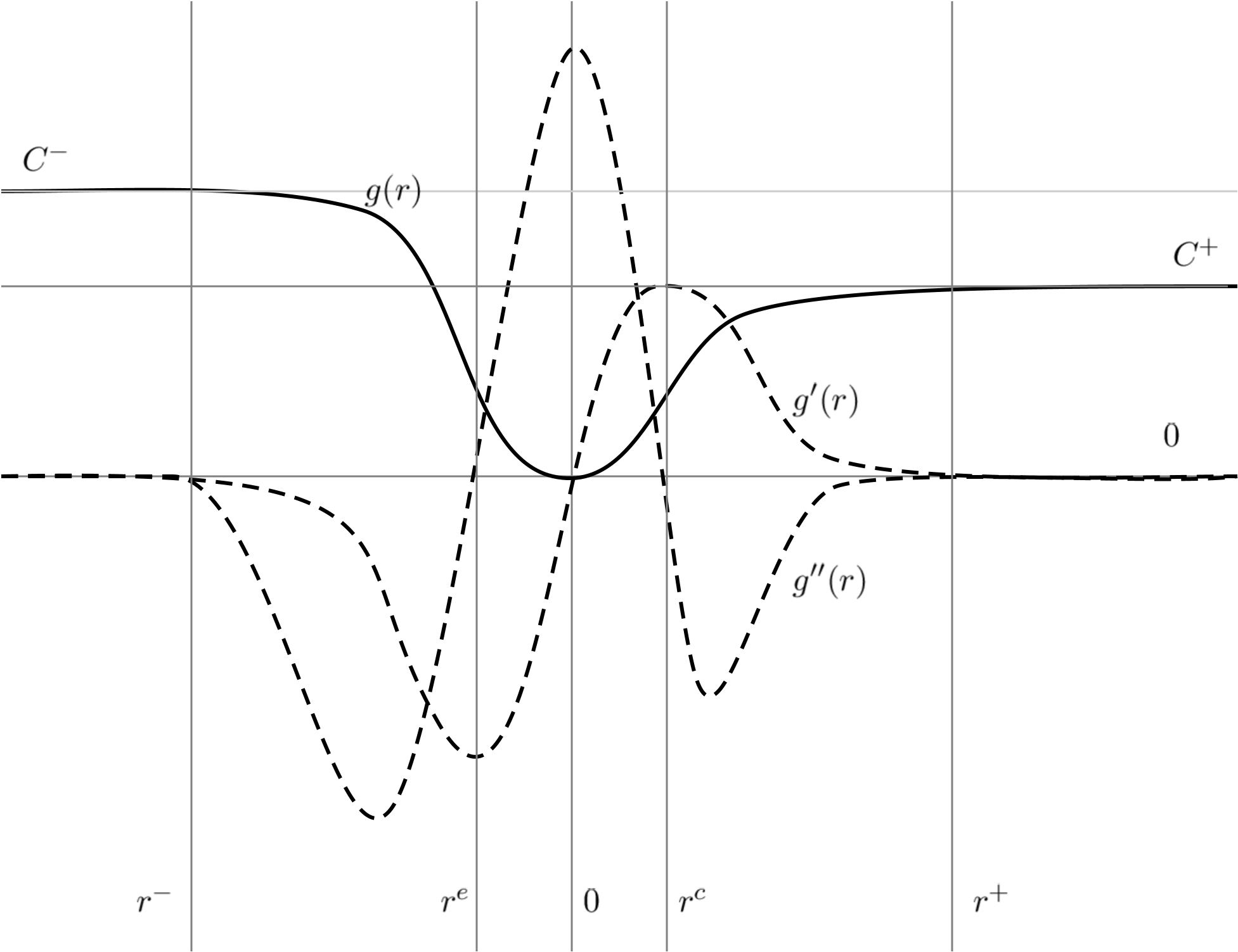
Figure 1: The double well potential function $g(r)$ and derivatives $g^{\prime}(r)$ and $g^{\prime\prime}(r)$ for tensile force. Here $C^{+}$ and $C^{-}$ are the asymptotic values of $g$. The derivative of the force potential goes smoothly to zero at $r^{+}$ and $r^{-}$.

The quasistatic evolution problem is now described. The load path is given by a prescribed body force density $\mathbf{b}(\mathbf{x},t)$ parameterized by $t$, with $0\leq t\leq T$ and written $\mathbf{b}(t)$. The associated displacement is written $\mathbf{u}(t):=\mathbf{u}(\mathbf{x},t)$. The application of $\mathbf{b}$ in the absence of prescribed boundary displacement is referred to as load control [anderson2017fracture]. We say that the displacement $\mathbf{u}(t)$ satisfies the quasi-static evolution problem for load control with prescribed load path $\mathbf{b}(t)$, $t\in[0,T]$ if it satisfies

(11) $$\mathcal{L}[\mathbf{u}(t)]=\mathbf{b}(t),$$

for $0\leq t\leq T$.

We conclude this section noting that in the peridynamic taxonomy our cohesive model is classified as a bond-based or ordinary state based peridynmic material model outlined in [silling2007peridynamic]. To see this write

(12) $$\mathcal{L}(\mathbf{u})=\int_{\Omega\cup\mathcal{H}_{\epsilon}(\mathbf{x})}\left({\mathbf{T}}(\mathbf{x})(\mathbf{y}-\mathbf{x})-\mathbf{T}(\mathbf{y})(\mathbf{x}-\mathbf{y})\right)\;d\mathbf{y},$$

where

(13) $$\mathbf{T}(\mathbf{y})(\mathbf{y}-\mathbf{x})=\partial_{S}\mathcal{W}^{\epsilon}(S(\mathbf{y},\mathbf{x},\mathbf{u}(t)))\mathbf{e}_{\mathbf{y}-\mathbf{x}},\mathbf{T}(\mathbf{x})(\mathbf{x}-\mathbf{y})=\partial_{S}\mathcal{W}^{\epsilon}(S(\mathbf{x},\mathbf{y},\mathbf{u}(t)))\mathbf{e}_{\mathbf{x}-\mathbf{y}}.$$

3 Existence and energy balance for load control

The section contains the main results and describes the existence and uniqueness of quasistatic evolution within a neighborhood of a prescribed initial deformation of the material. In what follows fixed point methods are applied to find solutions to the quasistatic evolution. Solutions are elements of a subspace of the well known Lebesgue space $L^{\infty}(\Omega;\mathbb{R}^{d})$ defined by all essentially bounded, measurable displacements with norm

(14) $$\|\mathbf{u}(t)\|_{\infty}:={\rm esssup}_{\mathbf{x}\in\Omega}|\mathbf{u}(\mathbf{x},t)|.$$

The $L^{2}(\Omega;\mathbb{R}^{d})$ norm is given by

(15) $$\|\mathbf{u}(t)\|_{2}:=\left(\int_{\Omega}\,|\mathbf{u}(\mathbf{x},t)|^{2}\,d\mathbf{x}\right)^{1/2}.$$

We remark at the outset that all positive constants that are independent of $\mathbf{u}$ are denoted either by $C$ or $K$ unless explicitly stated otherwise.

In what follows we denote a ball of radius $R$ centered at an element $\hat{\mathbf{u}}$ of
$L^{\infty}(\Omega;\mathbb{R}^{d})$ by,

(16) $$B(\hat{\mathbf{u}},R)=\left\{\mathbf{u}:\left\lVert\mathbf{u}-\hat{\mathbf{u}}\right\rVert_{\infty}\leq R\right\}.$$

The derivative of $\mathcal{L}$ at $\mathbf{u}$ is denoted by $D(\mathcal{L})[\mathbf{u}]$ and is a linear operator on $L^{\infty}(\Omega;\mathbb{R}^{d})$. The operator norm of $D(\mathcal{L})[\mathbf{u}]$ is written $\vvvert D(\mathcal{L})[\mathbf{u}]\vvvert$ and defined by

(17) $$\vvvert D(\mathcal{L})[\mathbf{u}]\vvvert=\sup_{\Delta\mathbf{u}\in L^{\infty}(\Omega;\mathbb{R}^{d})}\frac{\|D(\mathcal{L})[\mathbf{u}]\Delta\mathbf{u}\|_{\infty}}{\|\Delta\mathbf{u}\|_{\infty}}.$$

From Proposition 2 of section 4 the derivative is understood as a bounded linear map on $L^{\infty}(\Omega;\mathbb{R}^{d})$. For this case it is shown that there is a fixed positive constant $C>0$ independent of $\epsilon$ and $\Delta\mathbf{u}$ in $L^{\infty}(\Omega;\mathbb{R}^{d})$ such that

(18) $$\|D(\mathcal{L})[\mathbf{u}]\Delta\mathbf{u}\|_{\infty}\leq\frac{C}{\epsilon^{2}}\|\Delta\mathbf{u}\|_{L^{\infty}(\Omega;\mathbb{R}^{d})},$$

The inverse map when it exists on $\mathcal{V}$ is written $D(\mathcal{L})[\hat{\mathbf{u}}]^{-1}$ and

(19) $$\|D(\mathcal{L})[\mathbf{u}]^{-1}\Delta\mathbf{u}\|_{\infty}\geq\frac{\epsilon^{2}}{C}\|\Delta\mathbf{u}\|_{\infty}.$$

We define

(20) $$\vvvert D(\mathcal{L})[\mathbf{u}]^{-1}\vvvert=\sup_{\Delta\mathbf{u}\in\mathcal{V}}\frac{\|D(\mathcal{L})[\mathbf{u}]^{-1}\Delta\mathbf{u}\|_{\infty}}{\|\Delta\mathbf{u}\|_{\infty}}.$$

In this treatment we consider a very general class of domains $\Omega$. These are the domains that satisfy the interior cone condition [adams2003sobolev].

Definition 2.

The interior cone condition for $\Omega$ states that there exists a positive constant angle $\theta>0$ such that any $\mathbf{x}\in\Omega$ contains a spherical cone $C_{\lambda,\theta}(\mathbf{x},\mathbf{e}_{\mathbf{x}})$ with its apex at $\mathbf{x}$, radius $\lambda$ aperture angle $2\theta$ bisected by an axis in the direction of a unit vector $\mathbf{e}_{\mathbf{x}}$.

Such domains can not have external cusps, see Figure 2. Convex domains as well as non convex domains given by notched specimens satisfy the interior cone condition. In this treatment all domains $\Omega$ are assumed to satisfy the interior cone condition.

Figure 2: An example of a domain $\Omega$ that does not satisfy the interior cone condition.

We now identify the subspace of $L^{\infty}(\Omega;\mathbb{R}^{d})$ in which we find solutions to the load control problems. First let $\Pi$ denote the space of rigid motions, i.e.,

(21) $$\Pi=\{\mathbf{Q}\mathbf{x}+\mathbf{c}:\mathbf{Q}^{T}=-\mathbf{Q}\in\mathbb{R}^{d\times d},\mathbf{c}\in\mathbb{R}^{d}\}.$$

Direct use Lemma 2 of [DuGunLehZho] shows that the rigid rotations comprise the null space of the strain operator:

Proposition 1.

$S(\mathbf{y},\mathbf{x},\mathbf{u})=0$ for all $\mathbf{x}\in\Omega$ and $\mathbf{y}\in H_{\epsilon}(\mathbf{x})$ if and only if $\mathbf{u}\in\Pi$.

From this proposition it follows that $\mathcal{L}(\mathbf{w})=0$ if $\mathbf{w}\in\Pi$.

Denote the closure of $\mathcal{V}$ in $L^{2}(\Omega;\mathbb{R}^{d})$ by $\overline{\mathcal{V}}^{2}$. The function space $\mathcal{V}$ used for quasistatic evolutions under load control is given by;

Definition 3.

The space $\mathcal{V}\subset L^{\infty}(\Omega;\mathbb{R}^{d})$ is defined by

(22) $$\mathcal{V}=\{\mathbf{u}\in L^{\infty}(\Omega;\mathbb{R}^{d});\,\,\int_{\Omega}\mathbf{u}\cdot\mathbf{w}\,d\mathbf{x}=0,\hbox{ for all $\mathbf{w}\in\Pi$}\}.$$

This space is closed in the $L^{\infty}(\Omega;\mathbb{R}^{d})$ norm and it follows that $\overline{\mathcal{V}}^{2}\cap\Pi=\{\boldsymbol{0}\}$.

Lemma 3.1.

For $\mathbf{u}\in\mathcal{V}$ one has $\mathcal{L}[\mathbf{u}]\in\mathcal{V}$ and is a bounded operator.

This follows from the straight forward estimate $\|\mathcal{L}(\mathbf{u})\|_{\infty}\leq C\|\mathbf{u}\|_{\infty}$ and $\int_{\Omega}\mathcal{L}[\mathbf{u}]\cdot\mathbf{w}\,d\mathbf{x}=0$. The orthogonality follows from an integration by parts as in the proof of Lemma LABEL:thm:symmet of section LABEL:sec:symmbounded and Proposition 1.

The operator $\mathcal{L}[\mathbf{u}]$ is continuously Fréchet differentiable on $\mathcal{V}$.

Theorem 1.

The linear transform $D(\mathcal{L})[\mathbf{u}]:\mathcal{V}\rightarrow\mathcal{V}$ is the Fréchet derivative of $\mathcal{L}$ and exists with respect to the $L^{\infty}(\Omega;\mathbb{R}^{d})$ norm for all $\mathbf{u}\in\mathcal{V}$, i.e.,

(23) $$\lim_{\|\Delta\mathbf{u}\|_{\infty}\rightarrow 0}\frac{\|\mathcal{L}[\mathbf{u}+\Delta\mathbf{u}](\mathbf{x})-\mathcal{L}[\mathbf{u}](\mathbf{x})-D(\mathcal{L})[\mathbf{u}]\Delta\mathbf{u}\|_{\infty}}{\|\Delta\mathbf{u}\|_{\infty}}=0.$$

Moreover it is Lipshitz continuous in $\mathbf{u}$, i.e., for $\boldsymbol{\delta},\Delta\mathbf{u}\in\mathcal{V}$ there is a constant $C$ independent of $\boldsymbol{\delta}$ such that

(24) $$\frac{\|D(\mathcal{L})[\mathbf{u}+\boldsymbol{\delta}]\Delta\mathbf{u}-D(\mathcal{L})[\mathbf{u}]\Delta\mathbf{u}\|_{\infty}}{\|\Delta\mathbf{u}\|_{\infty}}\leq C\|\boldsymbol{\delta}\|_{\infty}.$$

The theorem is proved in section 4.

We now and assert the existence of solutions to the load control problem.

Theorem 2 (Load control).

Let $\mathbf{u}_{0},\mathbf{b}_{0}\in\mathcal{V}$ be such that $\mathcal{L}[\mathbf{u}_{0}]=\mathbf{b}_{0}$ and assume ${D(\mathcal{L})[\mathbf{u}_{0}]^{-1}}$ exists and is bounded on on $\mathcal{V}$, set

(25) $$R=\frac{C\epsilon^{\frac{5}{2}}}{\vvvert D(\mathcal{L})[\mathbf{u}_{0}]^{-1}\vvvert},$$

where $C$ is obtained from (LABEL:eq:const). Then for any given load path such that $\mathbf{b}(t):[0,T]\to\mathcal{V}$ is continuous and $\mathbf{b}(t)\in B\left(\mathbf{b}_{0},\frac{R}{2\vvvert D(\mathcal{L})[\mathbf{u}_{0}]^{-1}\vvvert}\right)$, there exists a unique continuous solution path $\mathbf{u}(t)\in\mathcal{V}$ lying inside $B(\mathbf{u}_{0},R)$ such that

(26) $$\mathcal{L}[\mathbf{u}(t)]=\mathbf{b}(t),\hbox{ for $t\in[0,T]$.}$$

We now show that $D(\mathcal{L})[\boldsymbol{\mathbf{u}}_{0}]^{-1}$ exists and is bounded on $\mathcal{V}$ for fields $\mathbf{u}_{0}$ inside the strength domain. This includes the case $\mathbf{u}_{0}=\boldsymbol{0}$. We now define the stability tensor.

Definition 3.

Stability tensor

(27) $$\mathbb{A}[\mathbf{u}](\mathbf{x})=\int\limits_{H_{\epsilon}(\mathbf{x})\cap\Omega}\frac{J^{\epsilon}(\left\lvert\mathbf{y}-\mathbf{x}\right\rvert)}{\epsilon^{d+1}\omega_{d}|\mathbf{y}-\mathbf{x}|}g^{\prime\prime}\left(\sqrt{\left\lvert\mathbf{y}-\mathbf{x}\right\rvert}S\left(\mathbf{y},\mathbf{x},\mathbf{u}\right)\right)\mathbf{e}_{\mathbf{y}-\mathbf{x}}\otimes\mathbf{e}_{\mathbf{y}-\mathbf{x}}d\mathbf{y}.$$

The stability tensor is a measurable tensor valued function. We write $\mathbb{A}[\mathbf{u}]-\gamma\mathbb{I}>0$ when for all $\mathbf{x}\in\Omega$ and all $\mathbf{v}\in\mathbb{R}^{d}$, $\mathbb{A}[\mathbf{u}](\mathbf{x})\mathbf{v}\cdot\mathbf{v}-\gamma|\mathbf{v}|^{2}>0$.

When the domain satisfies the interior cone condition and one has a deformation $\mathbf{u}_{0}$ inside the strength domain we have;

Theorem 4 (Invertibility).

Assume $\mathbf{u}_{0}$ lies strictly inside the strength domain, i.e., for all $\mathbf{x}\in\Omega$ and $\mathbf{y}\in\Omega\cap H_{\epsilon}(\mathbf{x})$ the strain $\sqrt{\mathbf{x}-\mathbf{y}}S(\mathbf{y},\mathbf{x},\mathbf{u}_{0})$ lies inside a closed interval contained inside the interval $(r^{e},r^{c})$, and if $\Omega$ satisfies the interior cone condition then $Ker\{D(\mathcal{L})[\mathbf{u}]\}=\{\boldsymbol{0}\}$ and there is a $\gamma>0$ for which $\mathbb{A}[\mathbf{u}_{0}]-\gamma\mathbb{I}>0$ so $D(\mathcal{L})[\mathbf{u}_{0}]^{-1}$ is well defined on $\mathcal{V}$ and $\vvvert D(\mathcal{L})[\mathbf{u}_{0}]^{-1}\vvvert<\infty$.

Now we show existence of a nontrivial initial data $(\mathbf{u}_{0},\mathbf{b}_{0})$. Pick any $\mathbf{u}_{0}\neq 0$ in the strength domain of the material and set $\mathbf{b}_{0}=\mathcal{L}[\mathbf{u}_{0}]$. Now follows from 2 and 4 that for any given load path such that $\mathbf{b}(t):[0,T]\to\mathcal{V}$ is continuous and $\mathbf{b}(t)\in B\left(\mathbf{b}_{0},\frac{R}{2\vvvert D(\mathcal{L})[\mathbf{u}_{0}]^{-1}\vvvert}\right)$, there exists a unique continuous solution path $\mathbf{u}(t)\in\mathcal{V}$ lying inside $B(\mathbf{u}_{0},R)$ such that

(28) $$\mathcal{L}[\mathbf{u}(t)]=\mathbf{b}(t),\hbox{ for $t\in[0,T]$.}$$

However even with this initial condition Theorem 2 does not prohibit a solution $\mathbf{u}(t)$ associated with a propagating crack like defect.

We introduce the peridynamic potential energy.

(29) $$PD[\mathbf{u}]=\int\limits_{\Omega}\int\limits_{H_{\epsilon}(\mathbf{x})\cap\Omega}\left\lvert\mathbf{y}-\mathbf{x}\right\rvert\mathcal{W}^{\epsilon}(S(\mathbf{y},\mathbf{x},\mathbf{u}))d\mathbf{y}d\mathbf{x}.$$

The total energy of the system is given by

(30) $$E[\mathbf{u}]=PD[\mathbf{u}]-\int\limits_{\Omega}\mathbf{u}\cdot\mathbf{b}_{0}\ d\mathbf{x}.$$

The critical point $\mathbf{u}_{0}$ for the total energy (30) is given by the solution to the Euler Lagrange equation

(31) $$DE[\mathbf{u}_{0}]=0$$

which is

$$\mathcal{L}[\mathbf{u}_{0}]=\mathbf{b}_{0}.$$

Theorem 5.

Assume $\mathbf{u}_{0}$ lies strictly inside the strength domain and is a critical point of the energy $E[\mathbf{u}]$ given by (30) for the choice $\mathbf{b}=\mathbf{b}_{0}$. Then

(32) $$E[\mathbf{u}]\geq E[\mathbf{u}_{0}],$$

over all displacements $\mathbf{u}$ in the strength domain within the ball $B(\mathbf{u}_{0},R)$.

The Theorem 5 is proved in section LABEL:sec:energyminimize.

On combining theorems 2, 4, and 5 we discover that a quasistatic PD evolution exists within a neighborhood of a local energy minimizer over displacements inside the strength the domain.

Theorem 6.

Assume $\mathbf{u}_{0}$ lies strictly inside the strength domain and is a critical point of the energy $E[\mathbf{u}]$ given by (30) for the choice $\mathbf{b}=\mathbf{b}_{0}$, Under the hypothesis of Theorem 4 we can choose ${R}$ given by (25) such that for any continuous load path $\mathbf{b}(t):[0,T]\to\mathcal{V}$ with $\mathbf{b}(t)\in B\left(\mathbf{b}_{0},\frac{R}{2\vvvert D(\mathcal{L})[\mathbf{u}_{0}]^{-1}\vvvert}\right)$, there exists a unique continuous solution path $\mathbf{u}(t)\in\mathcal{V}$ lying inside $B(\mathbf{u}_{0},R)$ such that

(33) $$\mathcal{L}[\mathbf{u}(t)]=\mathbf{b}(t),\hbox{ for $t\in[0,T]$.}$$

Here $\mathbf{u}_{0}$ is a critical point and minimizer of the energy $E[\mathbf{u}]$ for the choice $\mathbf{b}=\mathbf{b}_{0}$,

(34) $$E[\mathbf{u}]\geq E[\mathbf{u}_{0}],$$

over all displacements $\mathbf{u}$ belonging to the strength domain inside the ball $B(\mathbf{u}_{0},R)$.

The energy inequality (34) of Theorem 6 is proved in section LABEL:sec:energyminimize.

When $\mathbf{u}_{0}$ does not lie in the strength domain and $\Omega$ does not satisfy an interior cone condition then one can no longer assert the existence of a $\gamma>0$ such that $\mathbb{A}-\gamma\mathbb{I}>0$. With this in mind we present a necessary condition for the invertibility of $D(\mathcal{L})[\mathbf{u}_{0}]$.

Theorem 7 (Necessity condition for invertibility).

Given $\mathbf{u}_{0}\in\mathcal{V}$. If $D(\mathcal{L})[\mathbf{u}_{0}]^{-1}$ exists on $\mathcal{V}$ then $Ker\{\mathbb{A}[\mathbf{u}_{0}](\mathbf{x})\}=\{\boldsymbol{0}\}$ almost everywhere on $\Omega$.

This necessity condition is seen in the more general sufficient conditions for invertibility given in Theorem LABEL:esistence_of_inverse_in_strength_domain. Part of the sufficient conditions require that all eigenvalues of $\mathbb{A}[\mathbf{u}]$ lie outside an open interval containing $0$.

To prove the theorem we suppose $Ker\{\mathbb{A}[\mathbf{u}_{0}](\mathbf{x})\}\not=\{\boldsymbol{0}\}$ on a set $\mathcal{F}\subset\Omega$ of nonzero Lebesgue measure and proceed to construct an explicit sequence of nonzero elements $\{\mathbf{w}_{n}\}\in\mathcal{V}$ to show that $\|D(\mathcal{L})[\mathbf{u}_{0}]\mathbf{w}_{n}\|_{\infty}\rightarrow 0$ but that $\|\mathbf{w}_{n}\|_{\infty}=1$. This proves that $D(\mathcal{L})[\mathbf{u}_{0}]^{-1}$ is not defined on $\mathcal{V}$. The proof is given in section LABEL:sec:necessary.

When the load path $[0,T]\rightarrow\mathbf{b}(t)$ is differentiable and its derivative is continuous in $t$ then energy balance holds. This is codified in the following theorem.

Theorem 8 (Energy balance).

If $\mathbf{u}_{0},\mathbf{b}_{0}$ satisfy the hypotheses of theorem 2, $\mathbf{b}(t)$ is continuously differentiable with respect to $t$ and $D(\mathcal{L})[\mathbf{u}]^{-1}$ exists for all $\mathbf{u}\in\overline{B(\mathbf{u}_{0},R)}$, then the derivative $\frac{\partial\mathbf{u}(t,\mathbf{x})}{\partial t}$ belongs to $L^{\infty}(\Omega;\mathbb{R}^{3})$ and is continuous in $t$ and is related to the loading rate $\mathbf{b}_{t}$ by

(35) $$D(\mathcal{L})[\mathbf{u}(t)]^{-1}\left(\frac{\partial\mathbf{b}(t)}{\partial t}\right)=\frac{\partial\mathbf{u}(t)}{\partial t},$$

and we have the energy balance for $0<t<T$, given by

$$PD[\mathbf{u}(t)]-\int\limits_{\Omega}\mathbf{u}(t)\cdot\mathbf{b}(t)\ d\mathbf{x} =PD[\mathbf{u}_{0}]-\int\limits_{\Omega}\mathbf{u}_{0}\cdot\mathbf{b}_{0}\ d\mathbf{x}$$

$$-\int_{0}^{t}\int_{\Omega}\mathbf{u}(\tau)\cdot\mathbf{b}_{t}(\tau)\,d\mathbf{x}\,d\tau,$$

where $PD(\mathbf{u})$ is given by (29) and $\mathbf{b}_{t}$ is the derivative of $\mathbf{b}(t)$.

If instead of having existence of $D(\mathcal{L})[\mathbf{u}]^{-1}$ for all $\mathbf{u}\in\overline{B(\mathbf{u}_{0},R)}$, we only know that $D(\mathcal{L})[\mathbf{u}_{0}]^{-1}$ exists we can appeal to Banach’s Lemma to find a quasistatic evolution $\mathbf{u}(t)$ that satisfies the energy balance in the neighborhood of $\mathbf{u}_{0}$. This is illustrated in section LABEL:energybalance.

4 Existence theory for load control

In this section we give the proofs of theorem 1 and theorem 2. We first prove theorem 2 as theorem 1 follows from techniques developed in its proof. In order to prove theorem 2 we establish the necessary prerequisites. For a fixed $\mathbf{u}\in\mathcal{V}$ we define the linear transform $D(\mathcal{L})[\mathbf{u}]$ acting on $\Delta\mathbf{u}\in\mathcal{V}$ by

$$D(\mathcal{L})[\mathbf{u}]\Delta\mathbf{u}=$$

(36) $$-\int\limits_{H_{\epsilon}(\mathbf{x})\cap\Omega}\frac{J^{\epsilon}(\left\lvert\mathbf{y}-\mathbf{x}\right\rvert)}{\epsilon^{d+1}\omega_{d}}g^{\prime\prime}\left(\sqrt{\left\lvert\mathbf{y}-\mathbf{x}\right\rvert}S\left(\mathbf{y},\mathbf{x},\mathbf{u}\right)\right)S(\mathbf{y},\mathbf{x},\Delta\mathbf{u})\mathbf{e}_{\mathbf{y}-\mathbf{x}}d\mathbf{y},$$

and we first note that it a linear functional on $L^{\infty}(\Omega;\mathbb{R}^{2})$.

Proposition 2.

The linear functional $D(\mathcal{L})[\mathbf{u}]$ exists for all $\mathbf{u}\in\cal{V}$ and is a bounded linear functional for $\Delta\mathbf{u}\in L^{\infty}(\Omega;\mathbb{R}^{d})$.

Proof 4.1.

Recalling $g^{\prime\prime}(0)=\max\{|g^{\prime\prime}(r)|\}$ the proposition follows from the string of inequalities

$$\|D(-\mathcal{L})[\mathbf{u}]\Delta\mathbf{u}\|_{\infty}\leq$$

$${\rm esssup}_{\mathbf{x}\in\Omega}\{\int\limits_{H_{\epsilon}(\mathbf{x})\cap\Omega}|\frac{J^{\epsilon}(\left\lvert\mathbf{y}-\mathbf{x}\right\rvert)}{\epsilon^{d+1}\omega_{d}}g^{\prime\prime}\left(\sqrt{\left\lvert\mathbf{y}-\mathbf{x}\right\rvert}S\left(\mathbf{y},\mathbf{x},\mathbf{u}\right)\right)S(\mathbf{y},\mathbf{x},\Delta\mathbf{u})\mathbf{e}_{\mathbf{y}-\mathbf{x}}|d\mathbf{y}\}$$

$$\leq C\,{\rm esssup}_{\mathbf{x}\in\Omega}\{\frac{1}{\epsilon^{d+1}\omega_{d}}\int\limits_{H_{\epsilon}(\mathbf{x})\cap\Omega}\frac{|\Delta\mathbf{u}|}{|\mathbf{y}-\mathbf{x}|}d\mathbf{y}\}\leq\frac{C}{\epsilon^{2}}||\Delta\mathbf{u}||_{\infty},$$

where the constant $C$ is independent of $\Delta\mathbf{u}$ and $\epsilon.$

The existence of a quasistatic evolution is based on fixed point theory. We start by proposing a functional $T_{\mathbf{b}-\mathbf{b}_{0}}(\mathbf{u}-\mathbf{u}_{0})$ defined on $B(\mathbf{u}_{0},R)$ such that at its fixed point $\mathbf{u}^{\ast}-\mathbf{u}_{0}$ one has that $\mathcal{L}[\mathbf{u}^{\ast}]=\mathbf{b}$.

Proposition 3.

Define

(37) $$F_{\mathbf{u}_{0}}(\mathbf{u}-\mathbf{u}_{0})= -\mathcal{L}[(\mathbf{u}-\mathbf{u}_{0})+\mathbf{u}_{0}]+\mathcal{L}[\mathbf{u}_{0}]-D(-\mathcal{L})[\mathbf{u}_{0}](\mathbf{u}-\mathbf{u}_{0})$$

$$= -\mathcal{L}[\mathbf{u}]+\mathcal{L}[\mathbf{u}_{0}]-D(-\mathcal{L})[\mathbf{u}_{0}](\mathbf{u}-\mathbf{u}_{0})$$

and the map

(38) $$T_{\mathbf{b}-\mathbf{b}_{0}}(\mathbf{u}-\mathbf{u}_{0}) =-D(-\mathcal{L})[\mathbf{u}_{0}]^{-1}\left(F_{\mathbf{u}_{0}}(\mathbf{u}-\mathbf{u}_{0})+(\mathbf{b}-\mathbf{b}_{0})\right).$$

If $T_{\mathbf{b}-\mathbf{b}_{0}}(\mathbf{u}^{*}-\mathbf{u}_{0})=\mathbf{u}^{*}-\mathbf{u}_{0},$ then $\mathcal{L}[\mathbf{u}^{*}]=\mathbf{b}$.