11institutetext: V.A. Kovtunenko 22institutetext: Institute for Mathematics and Scientific Computing, Karl-Franzens University of Graz,
NAWI Graz, Heinrichstraße 36, 8010 Graz, Austria
22email: victor.kovtunenko@uni-graz.at and
Lavrentyev Institute of Hydrodynamics, Siberian Division of the Russian Academy of Sciences,
630090 Novosibirsk, Russia
33institutetext: K. Kunisch 44institutetext: Institute for Mathematics and Scientific Computing, Karl-Franzens University of Graz,
NAWI Graz, Heinrichstraße 36, 8010 Graz, Austria
44email: karl.kunisch@uni-graz.at and
Radon Institute, Austrian Academy of Sciences,
RICAM Linz, Altenbergerstraße 69, 4040 Linz, Austria
Shape Derivative for Penalty-Constrained Nonsmooth–Nonconvex Optimization: Cohesive Crack Problem
Victor A. Kovtunenko
Karl Kunisch
Abstract
A class of non-smooth and non-convex optimization problems with penalty constraints
linked to variational inequalities (VI) is studied with respect to its shape differentiability.
The specific problem stemming from quasi-brittle fracture describes
an elastic body with a Barenblatt cohesive crack under the inequality condition
of non-penetration at the crack faces.
Based on the Lagrange approach and using smooth penalization with the Lavrentiev
regularization, a formula for the shape derivative is derived.
The explicit formula contains both primal and adjoint states and is useful
for finding descent directions for a gradient algorithm
to identify an optimal crack shape from a boundary measurement.
Numerical examples of destructive testing are presented in 2D.
We develop a shape derivative of geometry-dependent least-squares
functions for a class of non-smooth and non-convex optimization problems.
The shape optimization problem is constrained by a penalty equation
linked to a variational inequality (VI).
The specific problem describes non-penetrating cracks with cohesion
in the framework of quasi-brittle fracture and destructive physical analysis (DPA).
Within the general theory for optimal control of VI Bar/84 ; MP/84 ,
the main challenge consists in the derivation of optimality conditions.
It can be studied by proper approximation of VI by regularized equations
and taking the limit as the regularization parameter tends to zero.
The corresponding methods for optimal control of obstacle problems
can be found in Ber/97 ; HHL/14 using augmented Lagrangians,
in e.g. HK/09 ; IK/03 for a Moreau–Yosida regularization, and in NT/09
based on a Lavrentiev regularization, for the latter see HKR/16 ; Lav/67 .
Furthermore we cite BLR/15 ; CCK/13 for control of non-smooth and non-convex
functionals, KV/07 for boundary control, and GJKS/18 ; ZMK/21
for control of quasi- and hemi-VI.
Shape optimization for free-interface identification with obstacle-type VI
using adjoints was developed recently by FSW/18 ; LSW/20 .
The common difficulty is a lack of regularity that needs
assumptions on a solution in order to take the limit Sch/22 .
Relying on linearized relations, a crack identification problem was treated e.g. in BB/13 .
We can refer also to ATS/21 ; HIIS/19 for relevant shape optimization
problems in acoustics, to GGK/21 in nonlinear flows subject to the divergence-free constraint,
to KO/20 for over-determined and to HKKP/03 for Bernoulli-type free boundary problems.
In the case of non-penetrating cracks (which are inequality-constrained),
the shape differentiability of the bulk energy was proved in
FHLRS/09 ; KK/00 for rectilinear cracks
and used for optimal shape design in KS/18 ; KMZ/08 ; LI/19 ; LSZ/15 .
For curvilinear cracks, adopting the theorem of
Correa–Seeger CS/85 on directional differentiability of Lagrangians
the shape derivative was derived in Kov/06 ; KK/07 ,
and in Rud/04 using -convergence.
For the non-penetrating Barenblatt crack that we investigate here,
the study of the objective function and its optimal control with respect to the crack shape
has a number of challenging tasks that we address below.
The subsequent Sections 3–7 follow Tasks (i)–(v),
which for convenience are summarized and explained in the following Sections 2.
2 Modeling tasks
Let by a parameter (time)-dependent geometry with
a crack along an interface (the breaking line) .
Denote by a normal vector to the surface .
Motivated by applications in fracture mechanics (see e.g. BMP/09 ), we consider
a total energy functional ,
which is given in a Hilbert space by the sum
(2.1)
where the bulk term is convex, typically, quadratic.
The term describes a surface energy according to
the Barenblatt idea of a cohesion zone and depends on the jump
expressing a possible discontinuity across the interface field .
The latter term is non-convex.
The condition of non-penetration (see KK/00 ; KS/97 ) for the normal opening
describes the feasible set
which is a convex cone.
For differentiable maps , the first order optimality condition
for the minimization of over
results in a VI
(2.2)
It constitutes a non-convex problem for a solid with a non-penetrating crack (see Kov/05 ).
For comparison, the classic Griffith model of brittle fracture
simplifies to be constant, and a crack
to be predefined at the interface .
This simplification results in a square-root singularity of the displacement
and infinite stress at the crack tip (front) .
This is the main disadvantage of the Griffith model,
we refer to CFMT/00 for a discussion.
A model, consistent with the physics of quasi-brittle fracture for non-constant
, was suggested by Barenblatt Bar/62 .
It takes into account the surface cohesion from the meso-level such that
the interface surfaces close in a smooth way, and thus allow healing of the crack.
Indeed, after solving problem (2.2) according to Barenblatt,
the set of points where an opening occurs, determines
the a-priori unknown crack along the interface .
This is the complement to the closed part of the interface where .
The main challenge of the direct problem (2.2) concerns
the term in (2.1).
From an optimization point of view, minimization over feasible
of with a non-smooth surface density
(when not a -function) leads to a hemi-VI (2.2).
The hemi-VI approach was analyzed theoretically and numerically
in HKK/11 ; OG/14 and used in Kov/11 ; KS/06 ; LPSS/13
to describe a quasi-static crack propagation.
A quadratic function describing adhesive cracks was studied in FIR/20 .
In the present paper, we study -smooth surface energies
that are small compared to the bulk term in (2.1),
see assumption (4.14) below, which is consistent with meso-level modeling.
Our ultimate aim is to identify the free-interface
by a shape optimization approach as described in GKK/20 .
For this task, we introduce the VI-constrained least-squares misfit from
a given measurement at an observation boundary :
(2.3)
where the regularization uses parameter .
This constitutes a nonsmooth–nonconvex optimization problem.
Our current work focuses on the following tasks.
Task (i): -approximation of .
To provide a shape derivative of defined in (2.3)
a continuously differentiable approximation of VI (2.2) is needed.
The standard penalization of non-penetration
by has only -regularity.
Here the regularization parameter is small, and
implies the decomposition into positive
and negative parts.
Therefore, we suggest a -penalization by the normal compliance
based on the Lavrentiev regularization
(see Theorem 4.1).
This results in a -approximation of for
the -approximation of (2.1)–(2.3) by
(2.4)
and the penalty equation involves the operator introduced as follows
(2.5)
Task (ii): adjoint-based optimality conditions.
Applying to the penalty-constrained least-square misfit (2.4) a Lagrange
multiplier approach (see IK/08 ), we can define an -dependent Lagrangian
as
(2.6)
The primal (inf-sup) problem: for fixed ,
find such that
(2.7)
Since is affine in ,
the first order optimality condition is given by
The dual (sup-inf) problem (see (ET/76, , Chapter 6)) reads:
for fixed ,
find such that
Note that with respect to is not a
linear continuous functional on the dual space .
The corresponding nonlinear optimization theory was developed
in e.g. IK/08 ; MZ/79 ; ZK/79 as follows.
If the variation with respect to in (2.5) exists,
and the associated adjoint operator
satisfying
is surjective with respect to , then the optimality condition is given by
(2.8)
For the abstract theory associated to adjoint operators we cite EL/13 ; Ibr/06 ; MAS/96 .
To justify (2.8), we shall linearize around the primal solution
to (2.7) (see Theorem 4.2) and suggest a suitable
linearized functional such that
(2.9)
Task (iii): shape derivative.
Our purpose is to calculate a shape derivative of the mapping
that is expressed by the one-sided limit (see DZ/11 ; SZ/92 ):
(2.10)
If a saddle-point
based on (2.7) and (2.9) exists, then the optimal value misfit
function defined in (2.4) is evidently equal to the optimal value Lagrange function
(2.11)
Henceforth, we have the following identity for the shape derivative according to (2.10):
(2.12)
In order to construct a proper ,
using a diffeomorphic coordinate transformation such that
(see (SZ/92, , Chapter 2)),
the bijection ,
provides the perturbed Lagrangian as
(2.13)
Then the results of Delfour–Zolesio DZ/11 on shape differentiabiliy
can be applied to justify the limit in (2.12),
see respective Theorem 5.1 and its Corollary 1.
Task (iv): limit as .
Taking the limit as in relations (2.11)
we shall prove the optimality conditions
(see Theorem 6.1 and its Corollary 3).
However, we cannot pass to the limit in (2.12) due to the presence
of the unbounded term .
We conjecture that the limit problem (2.2) is not differentiable.
This agrees with the assertion that VIs are not Fréchet differentiable
with respect to shape (see LSZ/15 ).
Therefore, in the numerical treatment we rely on the approximation (2.12)
with small for the shape derivative .
Task (v): shape optimization.
Commonly adopted in shape optimization, the gradient method needs
a descent direction minimizing the objective map
such that .
This can be attained by a proper choice of the transformation entering
implicitly in formula (2.12) (see Corollary 2).
Realizing the optimization algorithm for crack shape identification,
from our numerical tests we report the following feature.
Those parts of the crack faces which are in contact
(where the non-penetration constraint is active) are hidden from identification.
To identify a crack needs its faces to be open (that is, VI turns into unconstrained equation)
in accordance with the concept of destructive physical analysis (DPA).
3 Cohesive crack problem
We start with a detailed description of the geometry.
Let , , be a fixed hold-all domain
with Lipschitz boundary .
For the time-parameter , , we consider a parameter-dependent
geometry defined as follows.
For brevity we use a single notation for the collection of
geometric objects describing a broken domain
by means of the Dirichlet, Neumann, observation boundaries,
and the breaking line, respectively.
The outer boundary is split into two variable parts such that
and
with normal vector outward to .
The observation boundary is .
The domain is split into two variable sub-domains
with Lipschitz boundaries and outward
normal vectors such that at .
The conditions
and
are needed to guarantee the Korn–Poincare inequality.
These two domains are separated by a breaking manifold (the free-interface)
with normal direction
such that .
An example geometry of is sketched in 2D in Figure 1.
Figure 1: An example configuration of variable geometry in 2D.
We assume that these geometric properties are preserved for all
under suitable shape perturbations, which we specify below in Section 5.
For fixed , we consider a linear elastic body that occupies the disconnected domain
.
By this, -dimensional vectors of displacement at points
admit discontinuity across
resulting in the jump .
For further use we employ an orthogonal decomposition of admissible
into the normal component with factor and the tangential vector
at the interface such that
(3.1)
The latter inequality in (3.1) describes the non-penetration, see KK/00 .
The essential issue of modeling is to introduce a density at
for the surface energy in (2.1) that is consistent with physics.
Based on the decomposition (3.1), we set
(3.2)
The former, shear-induced term in (3.2), is associated with friction
between the crack surfaces.
Let the mapping ,
and its first and second derivatives be uniformly continuous functions, satisfying
for constants and all ,
(3.3)
For example, we have in mind a standard regularization of the Coulomb law
(see e.g. (SM/91, , Section 4.3.3)) with the positive, convex function
(3.4)
where is small, and is the friction bound.
In this case, , ,
and .
For convenience, the function in one variable
together with its first two derivatives are depicted in Figure 2.
Figure 2: Example graphics of in 1d.
The latter term in (3.2) associates cohesion between the crack surfaces.
Let
and its second derivative be uniformly continuous functions,
and let there exist constant such that
(3.5)
From the physics literature (e.g. Kit/08 ) we suggest
the following generic function
(3.6)
where is related to the fracture toughness,
and , are parameters.
In this case, and are proportional to .
The example of for is depicted in Figure 3.
Figure 3: Example graphics of as and .
In particular, the left plot in Figure 3 depicts the typical softening phenomenon
for growing .
It is worth noting that the left branch of for
implies a normal compliance and it is avoided
when the non-penetration in (3.1) holds.
The symmetric -by- tensors of linearized strain and
the Cauchy stress are given by
(3.7)
where for ,
the transposition swaps columns for rows.
A symmetric fourth order tensor of elastic coefficients
,
such that for ,
is positive definite and fulfills the Korn–Poincare inequality:
there exists such that
(3.8)
over the Sobolev space
(3.9)
For a boundary traction vector ,
we consider the following bulk energy
(3.10)
The feasible set corresponding to the non-penetration condition in (3.1) reads
(3.11)
which is a convex, closed cone.
Theorem 3.1 (Well-posedness of cohesive crack problem)
There exists a solution to the non-convex, constrained minimization problem:
find such that
(3.12)
where the total energy according to (3.2) and (3.10) is given by
(3.13)
The solution satisfies the first-order optimality condition (2.2) in the form of VI:
(3.14)
for all test functions .
For smooth solutions the boundary value relations hold:
(3.15)
for the decomposition of vector according to (3.1).
The last two lines in (3.1) are the complementarity conditions.
If both and were convex
(that is not in (3.6)),
then the solution to (3.12) and (3.14) would be unique.
Proof
On the right-hand side of (3.13), the first, quadratic in
integral term over , is strongly positive
by the Korn–Poincare inequality (3.8).
Using the Cauchy–Schwarz inequality, the other boundary integral terms over
and are bounded from below by a sub-linear in function
(3.16)
by virtue of the properties for , in (3.3), (3.5).
Therefore, estimating the jump by
and applying the trace inequality we have
(3.17)
Then we get that is radially unbounded, and thus coercive.
The functions and are uniformly continuous,
hence preserving -convergence (see BJ/61 ).
Using the compactness of the embedding of the traces of
at ,
from into , it follows that
the mapping from
is weakly lower semi-continuous.
Let , , be an infimal sequence in .
The coercivity of implies the boundedness of in .
Then, on a subsequence , there exists an accumulation point
such that weakly in
as .
By weak closedness of we have .
Taking the limit inferior of , the weak lower semi-continuity
of implies that attains the minimum in (3.12).
Applying standard variational arguments implies the optimality condition (3.14)
and (3.1), see details in (KK/00, , Section 1.4).
Moreover, if , were convex,
then the integral over in (3.13) is monotone.
This would lead to uniqueness of as solution to (3.14),
which is then necessarily the unique solution for (3.12).
∎
Next we approximate the VI (3.14) by a penalty method.
By itself penalization is a self-contained physical model allowing compliance,
see And/99 for the discussion.
4 Lavrentiev based regularization and saddle-point problem
Let .
For ,
the standard penalization of the inequality constraint by
has only a generalized derivative ,
where is the Heaviside step function such that
for , otherwise for .
We suggest a Lavrentiev based -regularization
by the normal compliance as follows.
Let the function
be concave and differentiable, with and uniformly continuous,
and let there exist such that
(4.1)
We assume that the following conditions hold, which describe relaxed complementarity
and compliance, respectively:
(4.2)
Figure 4: Example graphics of for fixed .
For example, we construct the following mollification of minimum function
(4.3)
which is depicted in Figure 4 together with its two derivatives.
Lemma 1
For from (4.3), the properties (4.1) and (4.2)
hold true with .
Moreover, implies that
decreases monotonically,
and is concave and increases monotonically.
Proof
The properties (4.1) can be easily checked.
To verify the first inequality in (4.2), from (4.3)
we deduce that for .
Here we use the complementary condition
and for .
We further have
according to the first estimate in (4.1).
Henceforth, after multiplication with ,
the lower bound
holds for .
Similarly,
for in (4.3),
and due to for .
The first estimate in (4.1), that is
,
after multiplication with
leads to the upper bound for .
This proves the second inequality in (4.2).
∎
Using Lemma 1 we obtain the existence result for the penalized cohesive crack problem.
Theorem 4.1 (Well-posedness of -regularized cohesive crack problem)
There exists a solution to the penalty problem:
find such that
(4.4)
for all test functions .
For smooth solutions the boundary value relations hold:
(4.5)
If both and were monotone,
then the solution to (4.4) would be unique.
Proof
We apply arguments similar to those in the proof of Theorem 3.1.
From the properties of in (3.3), and
from (3.5), the fact that
by (4.2),
and using the Cauchy–Schwarz, Korn–Poincare (3.8), and trace inequalities
(3.17), similarly to (3.16) we deduce the uniform lower bound
(4.6)
where
(4.7)
Therefore, the operator associated to (4.4), denoted following (2.5)
by ,
is coercive.
We have and
are uniformly continuous, and thus preserve -convergence,
the operator is weakly continuous in the following sense.
If weakly in
as (hence strongly in
by compactness),
then for each the following convergence holds
Therefore, applying a Galerkin approximation and the Brouwer fixed point theorem
(see Fra/94 ), a solution to the variational problem (4.4) can be argued.
Its uniqueness under the monotony assumption
(that is not in (3.6)),
and the boundary value formulation (4.1) can be derived in a standard way.
∎
Next, for a given observation , we consider
the -dependent least-squares misfit function from (2.4),
where satisfies (4.4):
(4.8)
From the fundamental theorem of calculus, we have the following representations
(4.9)
for differentiable .
Let us fix a solution to the variational equation (4.4).
Based on (4) we introduce a quadratic Lagrangian (compare to
in (2.6)) linearized around
(4.10)
and a saddle point problem corresponding to (2.11): for all ,
(4.11)
Then (4.8) can be expressed equivalently in the primal-dual form
(2.11) as
(4.12)
where according to (4) the optimal value of the Lagrangian at the solution is
(4.13)
Theorem 4.2 (Well-posedness of -regularized saddle-point problem)
Assume that the cohesion is small in the sense that constant
in (3.3), (3.5) are sufficiently small so that
(4.14)
where , are from (3.8), (3.17).
Then there exists a unique saddle-point
in (4.11).
Its primal component solves (4.4).
The dual component is a solution to the adjoint equation
corresponding to fixed :
(4.15)
for all test functions .
For smooth solutions the boundary value relations hold:
(4.16)
implying linear, Robin-type boundary conditions at the interface.
Proof
The saddle-point problem consists of two sub-problems:
the former and the latter inequalities in (4.11).
Since the Lagrangian from (4.10) is linear in ,
the primal maximization problem (the former inequality in (4.11))
is equivalent to the first order optimality condition (4.4).
Its solvability is proven in Theorem 4.1.
Since from (4.10)
is quadratic and convex in , the dual minimization problem
(the latter inequality in (4.11)) is the optimality condition
expressed by the adjoint equation (4.15).
Now we prove the solution existence for (4.15).
For fixed , the left-hand side of (4.15) forms
a linear continuous operator
.
Indeed, using the Cauchy–Schwarz inequality and the upper bounds for
, ,
in (3.3), (3.5), (4.1), the operator is bounded from above,
hence continuous.
Recalling the symmetry of the elasticity coefficients and
the Hessian matrix , the operator is self-adjoint.
Applying the Cauchy–Schwarz, Korn–Poincare (3.8) and trace inequalities
(3.17), due to the boundedness of ,
, in (3.3),
(3.5), (4.1), similarly to (4.6), we estimate uniformly from below
(4.17)
Here due to assumption (4.14).
In this case, is uniformly positive.
Because and are assumed uniformly continuous,
they preserve -convergence, and the operator
is weakly lower semi-continuous by
the compactness similar to arguments presented in the proof of Theorem 4.1.
According to the Lax–Milgram theorem, the variational equation (4.15)
has a unique solution.
We derive straightforwardly its boundary value formulation (4.2).
Since the variational equation (4.4) can be rewritten in the equivalent form
for all ,
by assumption (4.14) its solution is unique, too.
∎
5 Shape derivative
Let us fix a flow and its inverse
(5.1)
This defines an associated coordinate transformation and its inverse .
For every fixed , we suppose that for it forms a diffeomorphism
(5.2)
where the perturbed geometry
describes the broken domain .
From (5.1), a time-dependent kinematic velocity is assumed
defined by the formula
(5.3)
If a stationary velocity is given explicitly by
with at , thus preserving the hold-all domain,
then determines the flow (5.1) by unique solutions
to the autonomous ODE systems:
(5.4)
which build a semi-group of transformations.
The following properties (T1)–(T4) are needed to prove shape differentiability.
(T1)
We assume that
the map is bijective between the function spaces
(5.5)
Based on assumption (5.5), the perturbed objective
,
and Lagrangian ,
,
are well-defined for when
transformed to the reference geometry by setting
The set of saddle points
for (5.8) is a singleton for all , and as .
The proof is given in in Appendix B and
follows the arguments in the proof of Theorem 4.2, which treats
a particular case of the saddle-point problem (5.8) as .
Lemma 4 (T4)
There exists a subsequence as , such that
(5.19)
The proof of Lemma 4 is technical. It is presented in Appendix C.
Based on the properties (T1)–(T4) we establish the main result of this section.
Theorem 5.1 (Shape differentiability of -regularized
optimization problem)
Under assumption (4.14), the shape derivative (see its definition
(2.10) and existence criterion (2.12)) can be expressed
by the partial derivative from (5.16) as
Indeed, due to (T1)–(T4) all assumptions in Delfour–Zolesio
(DZ/11, , Chapter 10, Theorem 5.1) are satisfied.
Details of the proof can be found in KO/20 .
∎
Corollary 1 (Hadamard representation of the -dependent
shape derivative)
Assume that the solution of (4.4) and (4.15) satisfies
.
Introducing the decomposition into normal and tangential components according to
(5.21)
the following equivalent representation of the shape derivative (5.20)
holds in terms of boundary integrals in 2D:
(5.22)
where is a tangential vector at the boundary, and in 3D:
(5.23)
where is a binomial vector within the moving frame
at the respective boundary.
The terms in (5.22) and (5.23) are
(5.24)
with the curvature at .
The expressions along are defined by
We remark that the additional -regularity is available when a piecewise
-boundaries exclude singular points
(e.g. in 2D when the boundary parts meet each other with an -angle
as in Figure 1).
Corollary 2 (Descent direction for the -dependent optimization)
A descent direction for the perturbed in (5.15)
is provided by the following choice of the velocity
(5.27)
in 2D, and in 3D respectively
(5.28)
with , , and not all simultaneously equal to zero.
Proof
Direct substitution of (5.27) into (5.22) in 2D, respectively
(5.28) into (5.23) in 3D, provides that
.
∎
Corollary 2 is of practical importance since it provides well-posedness of
gradient schemes (see Algorithm 1) based on the descent direction from (5.27) and (5.28).
6 The limit as
In the following we derive the limit relations as .
We recall that all results involving the dual variable
assume that (4.14) holds true.
Lemma 5 (Uniform estimate)
The following a-priori estimate holds uniformly in :
(6.1)
Consequently, there exists a subsequence as
and an accumulation point such that
(6.2)
Proof
Passing due to the convergences (C.6) and (C.7) and using
the lower bound due to (4.2), in the limit
we improve the uniform a-priori estimate (C.5) and get (6.1).
Consequently (6.2) follows by a standard compactness argument.
Moreover, ensures
at , hence .
∎
Let be a solution to the VI (3.14) in Theorem 3.1.
According to (4.10) we introduce the -independent Lagrangian
as
(i)
There exists a pair
which satisfies the variational equation
(6.4)
for all test functions , simultaneously with the complementary relations
(6.5)
where stands for the duality pairing
between and its dual space .
The first component solves the VI (3.14),
and according to (3.1) the second, , satisfies
(6.6)
(ii)
Under the assumption (4.14), an adjoint pair exists and satisfies the adjoint equation
(6.7)
for all test functions , such that the compatibility relation holds:
(6.8)
where in (4.3) does not depend on .
In case is smooth, the following boundary value relations hold:
(6.9)
(iii)
The quadruple constitutes an accumulation point
as :
(6.10)
(6.11)
(6.12)
Proof
(i)
Taking the limit in (4.4) with the help of the weak convergence
in (6.2) we get
(6.13)
This implies the -weak convergence
in , equation (6.4), and
in (6.5) due to in Lemma 1.
Testing (6.13) with and using (4.2) such that
after passage , we get in the limit
.
On the other hand we have
because and the non-penetration ,
which together lead to the equality in (6.5).
Substituting with the expression (6.6) at
we derive the VI (3.14) and its boundary value formulation (3.1).
Thus, yields a solution of the cohesive crack problem.
(ii)
The limit of the adjoint equation (4.15) using the convergences in (6.2) is
(6.14)
The convergence in (6.14) implies (6.12) and the adjoint equation (6.7).
Derivation of the boundary value relations (6.1) is standard.
According to (4) we have
hence based on (6.11) and (6.12) we derive in the limit the compatibility
equation (6.8).
(iii)
The weak convergences in (6.10) are proved in Lemma 5.
To justify the strong convergence ,
we subtract (6.4) from (4.4), test the difference with
and rearrange the terms as follows
(6.15)
Using the monotony of and the uniform boundedness
for , the strong convergence in (6.10) follows
upon taking the limit in (6.15) as , see (6.2).
Consequently, from (4.4) and (6.13) we conclude the strong convergence in (6.11).
This finishes the proof.
∎
Based on assertion (iii) of Theorem 6.1 we get the following.
Corollary 3 (Limit optimization problems)
For the fixed
from Theorem 6.1 and Lagrangian from (6.3),
the pair solving optimality conditions
(6.4), (6.5) and (6.7) satisfies the primal problem:
(6.16)
for all , and the dual problem:
(6.17)
By the virtue of compatibility (6.8), the corresponding
optimal value function for the objective in (2.3)
has the equivalent representations using the adjoint equation as follows:
(6.18)
Proof
Indeed, taking the limit in the saddle-point problem (4.11)
with the Lagrangian from (4.13), and
observing (6.10)–(6.12), the inequalities (6.16), (6.17) follow.
From the -dependent representation (4.12)
of the optimal value function and by using the compatibility (6.8)
we derive the limit formula (6.18).
∎
We finish by noting the difficulty that, in general, we can pass to the limit
as neither in the term in the Lagrangian
in (4.10), nor in the term
in the shape derivative in (5.20) and (5.26).
Otherwise, if
exists, then the compatibility properties
and which are stronger than (6.8) hold.
For a factorization of and , additional solution
regularity, as in the particular case of obstacle problems, could be helpful,
see Bar/84 ; HK/09 ; MP/84 .
7 Shape optimization of breaking line
We apply the theoretical results to a numerical example in 2D.
As a true shape to be identified within an admissibility set
we take the piecewise-linear line
which breaks the rectangle into two parts .
Let the boundary be split symmetrically into the fixed Dirichlet
part and
the Neumann part .
For an isotropic elastic body occupying we set the material parameters:
Young modulus (mPa), Poisson ratio ,
and the corresponding Lamé parameters ,
.
For the matrix of isotropic elastic coefficients the stress-strain relations are
We rely on the approximation of by ,
and with
at , which is reasonable for flat shapes.
For a friction function in one variable
such that ,
and ,
applying to the body the traction force
according to Theorem 3.1 there exists a solution
such that on , ,
and satisfying the VI (3.14):
(7.1)
for all test functions
such that on and .
Let the observation boundary be .
We insert the solution of (7.1) as a measurement into the objective function
in (2.3) and consider the shape optimization problem:
find from the feasible set such that
(7.2)
Evidently, the trivial minimum in (7.2) is attained as
and .
To avoid the inverse crime, we use two different meshes for ,
and for when solving the inverse problem.
Now we discretize the problem.
For fixed , let , be triangular meshes
with grid size in , ,
which are compatible at the interface such that .
At the interface the nonlinear functions are set:
friction from (3.4) with (mPa);
cohesion from (3.6) with ,
(mPam), (m).
The parameters , are assumed sufficiently small
such that we rely on the discretization:
(7.3)
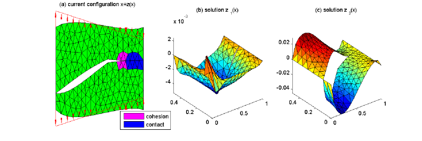
Figure 5: Computed true solution to (7.1)
within current configuration (a); componentwise in (b), (c).
After FE-discretization of problem (7.1) according to (7.3)
on a grid of size , we solve it by a primal-dual active set (PDAS)
iterative algorithm developed in HKK/11 .
The reference numerical solution obtained after 4 iterations
is plotted in Figure 5.
In plot (a) we present the grid in the so-called current or deformed configuration for
under the traction force prescribed at .
Here we observe an open part of which is the complement to
the cohesion part (where ) with contact (where )
marked by colors in finite elements adjacent to the interface.
In plots (b), (c) of Figure 5 the solution components ,
in the reference configuration are depicted.
According to Theorem 4.1 we approximate the VI (3.14)
by the -regularized cohesive crack problem (4.4).
For sufficiently small fixed, the compliance
from (4.3) is discretized as
(7.4)
Let be the finite element (FE) space of piecewise-linear functions such that
Then the discretization of the penalty equation (4.4) becomes:
find such that
(7.5)
and due to (7.3) the discrete adjoint equation (4.15) reads:
find such that
(7.6)
for all test functions .
After solving problems (7.5) and (7.6), since
and are fixed in this example,
according to Corollary 2 we calculate
at the moving boundary , and
at :
(7.7)
where is set,
by the virtue of (7.3), (7.4).
Relying on a flat shape approximation we take and
(7.8)
The discrete velocity at interface is defined on
a coarse grid of size .
According to Corollary 3 we get a descent direction by setting
and
(7.9)
where the scaling
is chosen, and the weight at
was found empirically as in GKK/20 .
Based on formulas (7.7)–(7.9) we formulate the shape optimization
algorithm of breaking line identification for the discretized version of (4.8) .
Algorithm 1 (breaking line identification)
(0)
Initialize the constant grid function at points .
Determine the line segment
, where
is the linear interpolate of ; set .
(1)
Set the interface and construct triangulations
, ;
find solutions ,
of the discrete penalty and adjoint equations (7.5), (7.6).
(2)
Calculate a velocity by formula (7.9);
update the grid function
(7.10)
From linear interpolation of determine the piecewise-linear segment
(7.11)
(3)
If stopping criterion holds, then STOP; else set and go to Step (1).
For 11 equidistant points as , the numerical result of Algorithm 1
after iterations (the stopping criterion) is depicted in Figure 6.
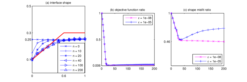
Figure 6: Iterations of (a);
objective function ratio (b);
shape error ratio (c).
In plot (a) the selected iterations of
from (7.11) are drawn in in comparison with
the true interface (the thick solid line).
In plot (b) of Figure 6 we plot the ratio
of the objective function during iterations
of , where we recall
(7.12)
The computed ratio attains as minimum .
In plot (c) of Figure 6 the ratio of shape error
is plotted versus ,
where according to (7.10)
(7.13)
Here the accuracy of shape identification attains only .
It is worth noting that the computation is presented for small penalty parameter
, while insufficiently small value
causes some increase of the ratio curves after reaching the minimum;
see Figure 6 (b), (c).
From the simulation we conclude the following.
In Figure 6 (a) it can be observed that the left part of
curve , where the constraints are inactive (see Figure 5 (a)),
is recovered well by the identification Algorithm 1,
whereas the right part of interface, where either contact or cohesion occurs,
the initialized is almost not modified during the iteration.
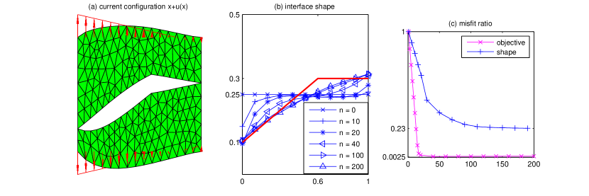
To remedy the hidden part, we apply to the same physical and geometrical configuration
the traction force ,
which is more stretching than the one from Figure 5 (a).
Because of that, the whole is open, neither contact nor cohesion occur
at the interface (see Figure 7 (a)).
The corresponding result of Algorithm 1 is depicted in Figure 7.
Figure 7: The true solution (a);
iterations of (b); objective function ratio and shape error ratio (c).
Here plot (b) presents the selected iterations of , and
plot (c) shows the objective function ratio
together with the shape error ratio .
The former ratio attains the minimum , and the latter one of accuracy.
Now we see in Figure 7 (b) that the whole curve
is recovered well compared to that from Figure 6 (a).
8 Conclusions
The Barenblatt’s crack model assuming cohesion at a breaking line
is stated as the variational inequality due to the non-penetration condition
and penalized using smooth Lavrentiev’s approximation.
For the geometry-dependent least-square function describing misfit
of the solution from a boundary measurement,
the expression of shape derivative is derived in an analytical form.
On its basis, from our numerical simulation we make a conclusion that
the suggested breaking line identification algorithm is consistent
within the setup of destructive physical analysis (DPA).
Data availability statement
Data sharing not applicable to this article as no datasets were generated or analysed during the current study.
Acknowledgements.
The research was supported by the ERC advanced grant 668998 (OCLOC) under the EU’s H2020 research program.
References
(1)
Alekseev, G.V., Tereshko, D.A., Shestopalov, Yu.V.:
Optimization approach for axisymmetric electric field cloaking and shielding.
Inverse Probl. Sci. Eng.49, 40–55 (2021)
(2)
Andersson, L.-E.:
A quasistatic frictional problem with a normal compliance penalization term.
Nonlinear Anal.37, 689–705 (1999)
(3)
Barbu, V.:
Optimal Control of Variational Inequalities,
Pitman, London (1984)
(4)
Barenblatt, G.I.:
The mathematical theory of equilibrium cracks in brittle fracture.
Adv. Appl. Mech.7, 55–129 (1962)
(5)
Bartle, R.G., Joichi, J.T.:
The preservation of convergence of measurable functions under composition.
Proc. Amer. Math. Soc.12 122–126 (1961)
(6)
Bellis, C., Bonnet, M.:
Qualitative identification of cracks using 3D transient elastodynamic
topological derivative: formulation and FE implementation.
Comput. Meth. Appl. Mech. Eng.253, 89–105 (2013)
(7)
Bergounioux, M.:
Use of augmented Lagrangian methods for the optimal control of obstacle problems.
J. Optim. Theory Appl.95, 101–126 (1997)
(8)
Bratov, V.A., Morozov, N.F., Petrov ,Yu.V.:
Dynamic Strength of Continuum,
St.Petersburg University (2009)
(9)
Bredies, K., Lorenz, D.A., Reiterer, S.:
Minimization of non-smooth, non-convex functionals by iterative thresholding.
J. Optim. Theory Appl.165, 78–112 (2015)
(10)
Casas, E., Clason, C., Kunisch, K.:
Parabolic control problems in measure spaces with sparse solutions.
SIAM J. Control Optim.51, 28–63 (2013)
(11)
Charlotte, M., Francfort, G., Marigo, J.-J., Truskinovsky, L.:
Revisiting brittle fracture as an energy minimization problem:
comparison of Griffith and Barenblatt surface energy models.
In: Benallal, A. (ed.): Continuous Damage and Fracture, pp. 1–12.
Elsevier, Paris (2000)
(12)
Correa, R., Seeger, A.:
Directional derivative of a minimax function.
Nonlinear Anal. Theory Methods Appl.9, 834–862 (1985)
(13)
Delfour, M.C., Zolésio, J.-P.:
Shape and Geometries: Metrics, Analysis, Differential Calculus, and Optimization,
SIAM, Philadelphia (2011)
(14)
Ekeland, I., Temam, R.:
Convex Analysis and Variational Problems,
North-Holland, Amsterdam (1976)
(15)
Estep, D., Lee, S.:
Adaptive error control during gradient search for an elliptic optimization problem.
Appl. Anal.92, 1434–1448 (2013)
(17)
Fremiot, G., Horn, W., Laurain, A., Rao, M., Sokolowski, J.:
On the Analysis of Boundary Value Problems in Nonsmooth Domains,
Dissertationes Mathematicae 462,
Inst. Math. Polish Acad. Sci., Warsaw (2009)
(18)
Führ, B., Schulz, V., Welker, K.:
Shape optimization for interface identification with obstacle problems.
Vietnam J. Math.46, 967–985 (2018)
(19)
Furtsev, A.I., Itou, H., Rudoy, E.M.:
Modeling of bonded elastic structures by a variational method:
Theoretical analysis and numerical simulation.
Int. J. Solids Struct.182-183, 100–111 (2020)
(20)
Ghilli, D., Kunisch, K., Kovtunenko, V.A.:
Inverse problem of breaking line identification by shape optimization.
J. Inverse Ill-posed Probl.28, 119–135 (2020)
(21)
González Granada, J.R., Kovtunenko, V.A.,
A shape derivative for optimal control of the nonlinear Brinkman–Forchheimer equation.
J. Appl. Numer. Optim.3, 243–261 (2021)
(22)
Gwinner, J., Jadamba, B., Khan, A.A., Sama, M.:
Identification in variational and quasi-variational inequalities.
J. Convex Anal.25, 545–569 (2018)
(23)
Haslinger, J., Kozubek, T., Kunisch, K., G. Peichl, G.:
Shape optimization and fictitious domain approach
for solving free boundary problems of Bernoulli type.
Comput. Optim. Appl.26, 231–251 (2003)
(24)
Hauptmann, A., Ikehata, M., Itou, H., Siltanen, S.:
Revealing cracks inside conductive bodies by electric surface measurements.
Inverse Probl.35, 025004 (2019)
(25)
Hintermüller, M., Hoppe, R.H.W., Löbhard, C.:
Use of augmented Lagrangian methods for the optimal control of obstacle problems.
ESAIM: COCV20, 524–546 (2014)
(26)
Hintermüller, M., Kovtunenko, V.A., Kunisch, K.:
Obstacle problems with cohesion: A hemi-variational inequality
approach and its efficient numerical solution.
SIAM J. Optim.21, 491–516 (2011)
(27)
Hintermüller, M., Kopacka, J.:
Mathematical programs with complementarity constraints in function space:
C- and strong stationarity and a path-following algorithm.
SIAM J. Control Optim.20, 868–902 (2009)
(29)
Ibragimov, N.H.:
Integrating factors, adjoint equations and Lagrangians.
J. Math. Anal. Appl.318, 742–757 (2006)
(30)
Ito, K., Kunisch, K.:
Semi-smooth Newton methods for state-constrained optimal control problems.
Systems Control Lett.50, 221–228 (2003)
(31)
Ito, K., Kunisch, K.:
Lagrange Multiplier Approach to Variational Problems and Applications,
SIAM, Philadelphia (2008)
(32)
Khludnev, A.M., Kovtunenko, V.A.:
Analysis of Cracks in Solids,
WIT-Press, Southampton, Boston (2000)
(33)
Khludnev, A.M., Shcherbakov, V.V.:
A note on crack propagation paths inside elastic bodies.
Appl. Math. Lett.79, 80–84 (2018)
(34)
Khludnev, A.M., Sokolowski, J.:
Modelling and Control in Solid Mechanics,
Birkhäuser, Basel (1997)
(35)
Kitamura, K.:
Crack surface energy: temperature and force dependence.
Materials Trans.49, 643–649 (2008)
(36)
Knees, D., Mielke, A., Zanini, C.:
On the inviscid limit of a model for crack propagation.
Math. Models Meth. Appl. Sci.18, 1529–1569 (2008)
(37)
Kovtunenko, V.A.:
Nonconvex problem for crack with nonpenetration.
Z. Angew. Math. Mech.85, 242–251 (2005)
(38)
Kovtunenko, V.A.:
Primal-dual methods of shape sensitivity analysis for curvilinear
cracks with non-penetration.
IMA J. Appl. Math.71, 635–657 (2006)
(39)
Kovtunenko, V.A.:
A hemivariational inequality in crack problems.
Optimization60, 1071–1089 (2011)
(40)
Kovtunenko, V.A., Kunisch, K.:
Problem of crack perturbation based on level sets and velocities.
Z. Angew. Math. Mech.87, 809–830 (2007)
(41)
Kovtunenko, V.A., Ohtsuka, K.:
Shape differentiability of Lagrangians and application to overdetermined problems.
In: Itou, H., Hirano, S., Kimura, M., Kovtunenko, V.A., Khludnev, A.M. (eds.):
Mathematical Analysis of Continuum Mechanics and Industrial Applications III
(Proc. CoMFoS18),
Ser. Mathematics for Industry 34, pp. 97–110, Springer, Singapur (2020)
(42)
Kovtunenko, V.A., Sukhorukov, I.V. :
Optimization formulation of the evolutionary problem
of crack propagation under quasibrittle fracture.
Appl. Mech. Tech. Phys.47, 704–713 (2006)
(43)
Kunisch, K., Vexler, B.:
Constrained Dirichlet boundary control in for a class of evolution equations.
SIAM J. Control Optim.46, 1726–1753 (2007)
(44)
Lavrentiev, M.M.:
Some Improperly Posed Problems of Mathematical Physics,
Springer, Berlin, Heidelberg (1967)
(45)
Lazarev, N., Itou, H.:
Optimal location of a rigid inclusion in equilibrium problems
for inhomogeneous Kirchhoff–Love plates with a crack.
Math. Mech. Solids24, 3743–3752 (2019)
(46)
Leugering, G., Prechtel, M., Steinmann, P., Stingl, M.:
A cohesive crack propagation model: mathematical theory and numerical solution.
Commun. Pure Appl. Anal.12, 1705–1729 (2013)
(47)
Leugering, G., Sokolowski, J., Zockowski, A.:
Shape- and topology optimization for passive control of crack propagation.
In: Pratelli, A., Leugering, G. (eds): New Trends in Shape Optimization.
Int. Ser. Numer. Math. 166, pp. 141–197, Birkhäluser, Cham (2015)
(48)
Luft, D., Schulz, V., Welker, K.:
Efficient techniques for shape optimization with variational inequalities using adjoints.
SIAM J. Optim.30, 1922–1953 (2020)
(49)
Marchuk, G.I., Agoshkov, V.I., Shutyaev, V.P.:
Adjoint Equations and Perturbation Algorithms in Nonlinear Problems,
CRC Press, Boca Raton (1996)
(50)
Maurer, H., Zowe, J.:
First and second-order necessary and sufficient optimality conditions
for infinite-dimensional programming problems.
Math. Program.16, 98–110 (1979)
(51)
Mignot, F., Puel, J.P.:
Optimal control in some variational inequalities.
SIAM J. Control Optim.22, 466–476 (1984)
(52)
Neitzel, I., Tröltzsch, F.:
On regularization methods for the numerical solution of parabolic
control problems with pointwise state constraints.
ESAIM: COCV15, 426–453 (2009)
(53)
Ovcharova, N., Gwinner, J.:
A study of regularization techniques of nondifferentiable optimization
in view of application to hemivariational inequalities.
J. Optim. Theory Appl.162, 754–778 (2014)
(54)
Rudoy, E.M.:
Differentiation of energy functionals in two-dimensional elasticity theory
for solids with curvilinear cracks.
J. Appl. Mech. Techn. Phys.54, 843–852 (2004)
(55)
Shcherbakov, V.V.:
Shape derivatives of energy and regularity of minimizers
for shallow elastic shells with cohesive cracks.
Nonlinear Anal. Real World Appl.65, 103505 (2022)
(56)
Sofonea, M., Matei, A.:
Mathematical Models in Contact Mechanics,
Cambridge Univ. Press (1991)
(58)
Zeng, S.D., Migórski, S., Khan, A.A.:
Nonlinear quasi-hemivariational inequalities: existence and optimal control.
SIAM J. Control Optim.59, 1246–1274 (2021)
(59)
Zowe, J., Kurcyusz, S.:
Regularity and stability for the mathematical programming problem in Banach spaces.
Appl. Math. Optim.5, 49–62 (1979)
As , the following asymptotic expansion of terms in (5.12)–(5.10)
holds (see e.g. (SZ/92, , Chapter 2)):
(A.1)
for .
It is worth noting that and
from (5.17) are just a notation used for short,
which does not require existence of the gradients here.
The tangential divergence is defined in (5.18).
Inserting representations (A.1) into the objective
and the perturbed Lagrangian
given by (5.9), (5.11), we derive their expansions
(5.14), (5.15) with respect to .
The asymptotic term
is from (5.16) at (implying that ).
Since and are continuous functions
of the argument , the partial derivative
in (5.16) is continuous.
This finishes the proof.
The first inequality in (5.8) implies the optimality condition
, that is
(B.1)
According to the asymptotic representation (5.15) and the mean value theorem,
using the operator from (4.15)
it is possible to express the equation (B.1) in the form
(B.2)
with a bounded, bilinear residual .
Under assumption (4.14) the operator
is coercive (see (4.17)) and weakly continuous.
Thus by the Brouwer fixed point theorem, for small the variational equation (B.2)
has a unique solution .
Similarly, the optimality condition
reads as
(B.3)
The second inequality in (5.8) admits the decomposition
for a weight :
(B.4)
with bounded bilinear ,
thus possesses a unique solution ,
for small enough.
Testing the variational equation (B.1) with
and applying the asymptotic expansion (B.2) it follows
(C.1)
We apply to (C.1) the Cauchy–Schwarz, Korn–Poincare (3.8)
and trace inequalities (3.17).
By the virtue of boundedness of , ,
, ,
and in (3.3), (3.5), (4.1),
we derive the estimate:
(C.2)
uniform in and for sufficiently small ,
where
due to the assumption (4.14).
Uniform estimate of .
We test the variational equation (B.3) with .
and apply (B.4):
(C.3)
With the help of Cauchy–Schwarz, Korn–Poincare and trace inequalities (3.8),
(3.17), due to the bondedness of ,
, in (3.3),
(3.5), (4.1), from (C.3) we derive the uniform estimate:
there exists such that
(C.4)
Thus, for small
relations (C.2) and (C.4) together give
(C.5)
Weak convergence of
.
By the virtue of the uniform estimate (C.5), there exists
a subsequence as , and a weak accumulation point
such that
(C.6)
By the compactness of embedding of the boundary traces it follows that
(C.7)
Next we take the limit in (B.1) and (B.3) with as . Due to the uniform
continuity of ,
and , , and
using (4) we arrive at the variational equations (4.4) and (4.15), respectively.
Therefore, .
Strong convergence of .
With the help of asymptotic relation (C.1) and equation (4.4)
with , using the Korn–Poincare inequality (3.8),
we rearrange the terms as follows
(C.8)
Taking the limit in (C.8) as , due to the convergence established in
(C.6) and (C.7), we conclude that
(C.9)
Strong convergence of .
We subtract equation (4.15) from (B.3) and use asymptotic expansions
(A.1) such that
(C.10)
Applying to (C.10) the Cauchy–Schwarz inequality, due to
the properties of , , in (3.3), (3.5), (4.1),
we obtain the upper bound
(C.11)
By the Sobolev embedding theorem the continuity property holds:
(C.12)
Then (C.12), Korn–Poincare and trace inequalities (3.8), (3.17),
together with convergences (C.6), (C.7) guarantee that for fixed :
Let be a solution to (4.4) and (4.15).
We integrate by parts the domain integral over
from (5.20) at so that
where we use the assumption at .
Using boundary conditions from (4.1), (4.2)
and the notation from (5.24) it follows that
(D.1)
After substitution of (D.1) into (5.20), the integrand
at is gathered in the expression:
(D.2)
In order to combine like terms, we exploit the calculus
(D.3)
With the help of (D.3), the gradient of the product due to friction term is calculated:
(D.4)
where at according to (3.1).
Similarly, we compute the gradient for the cohesive term
(D.5)
By (D.4) and (D.5), the integrand (D.2) is expressed as
(D.6)
Introducing for short the notation of
in (5.26) which is based on (D.6),
we rearrange the terms in the shape derivative in the form
(D.7)
Since the tangential velocity, its tangential divergence, and the curvature are equal to
(D.8)
for smooth the integration along a boundary
is given by the formula (see e.g. (SZ/92, , (2.125))):
(D.9)
In (D.9) is a tangential vector at
positively oriented to in 2D,
and is a binomial vector
within the moving frame at in 3D.
Applying (D.9) to (D.7), decomposing the vectors
in (5.21) into the normal and tangential components, and recalling that
at ,
we conclude with the assertion of Corollary 1.