Joint Distribution Matters: Deep Brownian Distance Covariance for
Few-Shot Classification

Abstract

Few-shot classification is a challenging problem as only very few training examples are given for each new task. One of the effective research lines to address this challenge focuses on learning deep representations driven by a similarity measure between a query image and few support images of some class. Statistically, this amounts to measure the dependency of image features, viewed as random vectors in a high-dimensional embedding space. Previous methods either only use marginal distributions without considering joint distributions, suffering from limited representation capability, or are computationally expensive though harnessing joint distributions. In this paper, we propose a deep Brownian Distance Covariance (DeepBDC) method for few-shot classification. The central idea of DeepBDC is to learn image representations by measuring the discrepancy between joint characteristic functions of embedded features and product of the marginals. As the BDC metric is decoupled, we formulate it as a highly modular and efficient layer. Furthermore, we instantiate DeepBDC in two different few-shot classification frameworks. We make experiments on six standard few-shot image benchmarks, covering general object recognition, fine-grained categorization and cross-domain classification. Extensive evaluations show our DeepBDC significantly outperforms the counterparts, while establishing new state-of-the-art results. The source code is available at http://www.peihuali.org/DeepBDC.

1 Introduction

Few-shot classification [17, 15] is concerned with a task where a classifier can be adapted to distinguish classes unseen previously, given only a very limited number of examples of these classes. This is a challenging problem as scarcely labeled examples are far from sufficient for learning abundant knowledge and also likely lead to overfitting. One practical solution is based on the technique of meta-learning or learning to learn [39, 12], in which the episodic training is formulated to transfer the knowledge obtained on a massive meta-training set spanning a large number of known classes to the few-shot regime of novel classes. Among great advances that have been made, the line of metric-based methods attracts considerable research interest [15, 39, 33, 26], achieving state-of-the-art performance [47, 45] in recent years.

The primary idea of the metric-based few-shot classification is to learn representations through deep networks, driven by the similarity measures between a query image and few support images of some class [33, 47]. Statistically, the features of a query image (resp., support images) can be viewed as observations of a random vector $X$ (resp., $Y$) in a high-dimensional embedding space. Therefore, the similarity between images can be measured by means of probability distributions. However, modeling distributions of high-dimensional (and often few) features is hard and a common method is to model statistical moments. ProtoNet [33] and its variants (e.g., [26]) represent images by first moment (mean vector) and use Euclidean distance or cosine similarity for metric learning. To capture richer statistics, several works study second moment (covariance matrix) [44] or combination of first and second moments in the form of Gaussians [20] for image representations, while adopting Frobenius norm or Kullback-Leiberler (KL) divergence as similarity measures. However, these methods only exploit marginal distributions while neglecting joint distributions, limiting the performance of learned models. In addition, the covariances can only model linear relations.

Method	Probability model	Dis-similarity$/$similarity measure	Joint	Dependency	Latency	Accuracy (%)
			distribution			1-shot	5-shot
ProtoNet [33]	Mean vector	$\|\boldsymbol{\upmu}_{X}-\boldsymbol{\upmu}_{Y}\|^{2}$  or  $\frac{\boldsymbol{\upmu}_{X}^{T}\boldsymbol{\upmu}_{Y}}{\|\boldsymbol{\upmu}_{X}\|\|\boldsymbol{\upmu}_{Y}\|}$	No	N/A	Low	49.42	68.20
CovNet [44]	Covariance matrix	$\|\boldsymbol{\Sigma}_{X}-\boldsymbol{\Sigma}_{Y}\|^{2}$	No	Linear	Low	49.64	69.45
ADM [20]	Gaussian distribution	$D_{\mathrm{KL}}(\mathcal{N}_{\boldsymbol{\upmu}_{X},\boldsymbol{\Sigma}_{X}}||\mathcal{N}_{\boldsymbol{\upmu}_{Y},\boldsymbol{\Sigma}_{Y}})$	No	N/A	Low	53.10	69.73
DeepEMD [47]	Discrete distribution	$\min_{f_{\mathbf{x}_{j},\mathbf{y}_{l}}\geq 0}\sum_{j}\!\!\sum_{l}f_{\mathbf{x}_{j},\mathbf{y}_{l}}c_{\mathbf{x}_{j},\mathbf{y}_{l}}$ $\mathrm{s.t.}\;\sum_{l}\!f_{\mathbf{x}_{j},\mathbf{y}_{l}}\!\!=\!\!f_{\mathbf{x}_{j}},\sum_{j}\!f_{\mathbf{x}_{j},\mathbf{y}_{l}}\!\!=\!\!f_{\mathbf{y}_{l}}$ for $\forall j,l$	Yes	N/A	High	65.91	82.41
DeepBDC (ours)	Characteristic function	$\bigintsss_{\mathbb{R}^{p}}\!\!\!\bigintsss_{\mathbb{R}^{q}}\!\!\!\dfrac{|\phi_{XY}(\mathbf{t},\mathbf{s})\!-\!\phi_{X}(\mathbf{t})\phi_{Y}(\mathbf{s})|^{2}}{c_{p}c_{q}\|\mathbf{t}\|^{1+p}\|\mathbf{s}\|^{1+q}}d\mathbf{t}d\mathbf{s}$	Yes	Nonlinear & Independence	Low	67.34	84.46

Table 1: Comparison between our DeepBDC and the counterparts. To quantify the dependency between random vectors $X$ and $Y$, moments based methods [33, 44, 20] only model marginal distributions, suffering from limited representation capability; though achieving state-of-the-art performance by considering joint distributions, DeepEMD [47] is computationally expensive. Our DeepBDC measures discrepancy between joint characteristic function and product of the marginals, which can be efficiently computed in closed-form, and model non-linear relations and fully characterizes independence. Note that for a random vector its characteristic function and probability distribution are equivalent in that they form a Fourier transform pair. Here we report accuracies of 5-way 1-shot$/$5-shot classification on $mini$ImageNet; our result is obtained by Meta DeepBDC and results of the counterparts are duplicated from respective papers.

In general, the dependency between $X$ and $Y$ should be measured in light of their joint distribution $f_{XY}(\mathbf{x},\mathbf{y})$ [6]. Earth Mover’s Distance (EMD) is an effective method for measuring such dependency. As described in [29, Sec. 2.3], EMD seeks an optimal joint distribution $f_{XY}(\mathbf{x},\mathbf{y})$, whose marginals are constrained to be given $f_{X}(\mathbf{x)}$ and $f_{Y}(\mathbf{y})$, so that the expectation of transportation cost is minimal. In few-shot classification, DeepEMD [47] proposes differential EMD for optimal matching of image regions. Though achieving state-of-the-art performance, DeepEMD is computationally expensive [45], due to inherent linear programming algorithm. Mutual information (MI) [3, 28] is a well-known measure, which can quantify the dependency of two random variables by KL-divergence between their joint distribution and product of the marginals. Unfortunately, computation of MI is difficult in real-valued, high-dimensional setting [2], and often involves difficult density modeling or lower-bound estimation of KL-divergence [14].

In this paper, we propose a deep Brownian Distance Covariance (DeepBDC) method for few-shot classification. The BDC metric, first proposed in [36, 35], is defined as the Euclidean distance between the joint characteristic function and product of the marginals. It can naturally quantify the dependency between two random variables. For discrete observations (features), the BDC metric is decoupled so that we can formulate BDC as a pooling layer, which can be seamlessly inserted into a deep network, accepting feature maps as input and outputting a BDC matrix as an image representation. In this way, the similarity between two images is computed as the inner product between the corresponding two BDC matrices. Therefore, the core of our DeepBDC is highly modular and plug-and-play for different methodologies of few-shot image classification. Specifically, we instantiate our DeepBDC in meta-learning framework (Meta DeepBDC), and in the simple transfer learning framework relying non-episodic training (STL DeepBDC). Contrary to covariance matrices, our DeepBDC can freely handle non-linear relations and fully characterize independence. Compared to EMD, it also considers joint distribution and above all, can be computed analytically and efficiently. Unlike MI, the BDC requires no density modeling. We present differences between our BDC and the counterparts in Tab. 1.

Our contributions are summarized as follows. (1) For the first time, we introduce Brownian distance covariance (BDC), a fundamental but largely overlooked dependency modeling method, into deep network-based few-shot classification. Our work suggests great potential and future applications of BDC in deep learning. (2) We formulate DeepBDC as a highly modular and efficient layer, suitable for different few-shot learning frameworks. Furthermore, we propose two instantiations for few-shot classification, i.e., Meta DeepBDC based on the meta-learning framework with ProtoNet as a blue print, and STL DeepBDC based on simple transfer learning framework without episodic training. (3) We perform thorough ablation study on our methods and conduct extensive experiments on six few-shot classification benchmarks. The experimental results demonstrate that both of our two instantiations achieve superior performance and meanwhile set new state-of-the-arts.

2 Related Works

Representation learning in few-shot classification The image representation and the similarity measure play important roles in few-shot classifications where only limited labeled examples are available. In light of the image representation, we can roughly divide the few-shot classification methods into two categories. In the first category, the image representations are based on distribution modeling. They use either first moment (mean vector) [33], second moment (covariance matrix) [44] , Gaussian distribution [20] or discrete probability [47], and, accordingly, adopts Euclidean distance (or cosine similarity), Frobenious norm, KL-divergence or Earther Mover’s Distance as dis-similarity measures. The second category is concerned with feature reconstruction between the query image and the support images, by means of either directly linear reconstruction through Ridge regression [45] or attention mechanism [9, 46], or concerned with designing relational module to learn a transferable deep metric [34, 48]. Our methods belong to the first category, and the biggest difference from existing works is that we use Brownian Distance Covariance for representation learning in the few-shot regime.

Meta-learning versus simple transfer learning Meta-learning is a de facto framework for few-shot classification [39, 12]. It involves a family of tasks (episodes) split into disjoint meta-training and meta-testing sets. Typically, each task is formulated as a $N$-way $K$-shot classification, which spans $N$ classes each provided with $K$ support images and some query images. The meta-training and meta-testing sets share the episodic training strategy that facilitates generalization ability across tasks. Most of the methods, either optimization-based [12, 30] or metric-based [33, 34], follow this methodology. A lot of studies [47, 45, 5] have shown that, rather than meta-training from scratch, pre-training on the whole meta-training set is helpful for meta-learning. Recently, it has been found that simple transfer learning (STL) framework, which does not rely on episodic training at all, achieves very competitive performance [4, 8, 37]. For STL methods, during meta-training a deep network is trained for a common classification problem via standard cross-entropy loss on the whole meta-training set spanning all classes; during meta-testing, the trained model is used as an embedding model for feature extraction, then a linear model, such as a soft-max classifier [4, 8] or logistic regression model [37], is constructed and trained for the few-shot classification.

Finally, we mention that scarce works have ever used BDC in machine learning or computer vision, and so far we find one BDC-based dimension reduction method [7] which is not concerned with deep learning.

3 Proposed Method

In this section, we first introduce Brownian distance covariance (BDC). Then we formulate our DeepBDC in the convolutional networks. Finally, we instantiate our DeepBDC for few-shot image classification.

3.1 Brownian Distance Covariance (BDC)

The theory of BDC is first established in [36, 35] in light of characteristic function. The characteristic function of a random vector is equivalent to its probability density function (PDF), as they form a Fourier transform pair.

Let $X\in\mathbb{R}^{p},Y\in\mathbb{R}^{q}$ be random vectors of dimension $p$ and $q$, respectively, and let $f_{XY}(\mathbf{x},\mathbf{y})$ be their joint PDF. The joint characteristic function of $X$ and $Y$ is defined as

$$\!\!\!\!\phi_{XY}(\mathbf{t},\mathbf{s})\!=\!\!\!\int_{\mathbb{R}^{p}}\!\!\int_{\mathbb{R}^{q}}\!\!\exp(\!i(\mathbf{t}^{T}\mathbf{x}\!+\!\mathbf{s}^{T}\mathbf{y}))f_{XY}(\mathbf{x},\mathbf{y})d\mathbf{x}d\mathbf{y}$$ (1)

where $i$ is the imaginary unit. Clearly, the marginal distributions of $X$ and $Y$ are respectively $\phi_{X}(\mathbf{t})\!\!=\!\!\phi_{XY}(\mathbf{t},\mathbf{0})$ and $\phi_{Y}(\mathbf{s})\!\!=\!\!\phi_{XY}(\mathbf{0},\mathbf{s})$ where $\mathbf{0}$ is a vector whose elements are all zero. From theory of probability, we know $X$ and $Y$ are independent if and only if $\phi_{XY}(\mathbf{t},\mathbf{s})\!\!=\!\!\phi_{X}(\mathbf{t})\phi_{Y}(\mathbf{s})$. Provided $X$ and $Y$ have finite first moments, the BDC metric is defined as

$$\rho(X,Y)\!=\!\int_{\mathbb{R}^{p}}\!\!\int_{\mathbb{R}^{q}}\!\!\dfrac{|\phi_{XY}(\mathbf{t},\mathbf{s})-\phi_{X}(\mathbf{t})\phi_{Y}(\mathbf{s})|^{2}}{c_{p}c_{q}\|\mathbf{t}\|^{1+p}\|\mathbf{s}\|^{1+q}}d\mathbf{t}d\mathbf{s}$$ (2)

where $\|\cdot\|$ denotes Euclidean norm, $c_{p}=\pi^{(1+p)/2}/\Gamma((1+p)/2)$ and $\Gamma$ is the complete gamma function.

For the set of $m$ observations $\{(\mathbf{x}_{1},\mathbf{y}_{1}),\ldots,(\mathbf{x}_{m},\mathbf{y}_{m})\}$ which are independent and identically distributed (i.i.d.), a natural approach is to define the BDC metric in light of the empirical characteristic functions:

$$\phi_{XY}(\mathbf{t},\mathbf{s})=\frac{1}{m}\sum_{k=1}^{m}\exp(i(\mathbf{t}^{T}\mathbf{x}_{k}+\mathbf{s}^{T}\mathbf{y}_{k}))$$ (3)

Though Eq. (2) seems complicated, the BDC metric has a closed form expression for discrete observations. Let $\widehat{\mathbf{A}}\!=\!(\widehat{a}_{kl})\!\in\!\mathbb{R}^{m\times m}$ where $\widehat{a}_{kl}\!=\!\|\mathbf{x}_{k}\!-\!\mathbf{x}_{l}\|$ be an Euclidean distance matrix computed between the pairs of observations of $X$. Similarly, we compute the Euclidean distance matrix $\widehat{\mathbf{B}}\!=\!(\widehat{b}_{kl})\!\in\!\mathbb{R}^{m\times m}$ where $\widehat{b}_{kl}\!=\!\|\mathbf{y}_{k}\!-\!\mathbf{y}_{l}\|$. Then the BDC metric has the following form [35] :

$$\rho(X,Y)=\mathrm{tr}\big{(}\mathbf{A}^{T}\mathbf{B}\big{)}$$ (4)

where $\mathrm{tr}(\cdot)$ denotes matrix trace, $T$ denotes matrix transpose, and $\mathbf{A}=(a_{kl})$ is dubbed BDC matrix. Here $a_{kl}=\widehat{a}_{kl}-\frac{1}{m}\sum_{k=1}^{m}\widehat{a}_{kl}-\frac{1}{m}\sum_{l=1}^{m}\widehat{a}_{kl}-\frac{1}{m^{2}}\sum_{k=1}^{m}\sum_{l=1}^{m}\widehat{a}_{kl}$, where the last three terms indicate means of the $l$-th column, $k$-th row and all entries of $\widehat{\mathbf{A}}$, respectively. The matrix $\mathbf{B}$ can be computed in a similar manner from $\widehat{\mathbf{B}}$. As a BDC matrix is symmetric, $\rho(X,Y)$ can also be written as the inner product of two BDC vectors $\mathbf{a}$ and $\mathbf{b}$, i.e.,

$$\rho(X,Y)=\big{<}\mathbf{a},\mathbf{b}\big{>}=\mathbf{a}^{T}\mathbf{b}$$ (5)

where $\mathbf{a}$ (resp., $\mathbf{b}$) is obtained by extracting the upper triangular portion of $\mathbf{A}$ (resp., $\mathbf{B}$) and then performing vectorization.

The metric $\rho(X,Y)$ has some desirable properties. (1) It is non-negative, and is equal to 0 if and only if $X$ and $Y$ are independent. (2) It can characterize linear and non-linear dependency between $X$ and $Y$. (3) It is invariant to individual translations and orthonormal transformations of $X$ and $Y$, and equivariant to their individual scaling factors. That is, for any vectors $\mathbf{c}_{1}\in\mathbb{R}^{p},\mathbf{c}_{2}\in\mathbb{R}^{q}$, scalars $s_{1},s_{2}$ and orthonormal matrices $\mathbf{R}_{1}\in\mathbb{R}^{p\times p},\mathbf{R}_{2}\in\mathbb{R}^{q\times q}$, $\rho(\mathbf{c}_{1}+s_{1}\mathbf{R}_{1}X,\mathbf{c}_{2}+s_{2}\mathbf{R}_{2}Y)=|s_{1}s_{2}|\rho(X,Y)$.

3.2 Formulation of DeepBDC as a Pooling Layer

In terms of Eq. (4) and Eq. (5), we can see that the BDC metric is decoupled in the sense that we can independently compute the BDC matrix for every input image. Specifically, we design a two-layer module suitable for a convolutional network, which performs dimension reduction and computation of the BDC matrix, respectively. As the size of a BDC matrix increases quadratically with respect to the number of channels (feature maps) in the network, we insert a $1\times 1$ convolution layer for dimension reduction right after the last convolution layer of the network backbone.

Suppose the network (including the dimension reduction layer) is parameterized by $\boldsymbol{\uptheta}$ which embeds a color image $\mathbf{z}\in\mathbb{R}^{3}$ into a feature space. The embedding of the image is a $h\times w\times d$ tensor, where $h$ and $w$ are spatial height and width while $d$ is the number of channels. We reshape the tensor to a matrix $\mathbf{X}\in\mathbb{R}^{hw\times d}$, and can view either each column $\boldsymbol{\chi}_{k}\in\mathbb{R}^{hw}$ or each row (after transpose) $\mathbf{x}_{j}\in\mathbb{R}^{d}$ as an observation of random vector $X$. We mention that in practice, for either case the i.i.d. assumption may not hold, and comparison of the two options is given in Sec. 4.2.

In what follows, we take for example $\boldsymbol{\chi}_{k}$ as a random observation. We develop three operators, which successively compute the squared Euclidean distance matrix $\widetilde{\mathbf{A}}=(\tilde{a}_{kl})$ where $\tilde{a}_{kl}$ is squared Euclidean distance between the $k$-th column and $l$-th column of $\mathbf{X}$, the Euclidean distance matrix $\widehat{\mathbf{A}}=(\sqrt{\widetilde{a}_{kl}})$, and the BDC matrix $\mathbf{A}$ obtained by subtracting from $\widehat{\mathbf{A}}$ its row mean, column mean and mean of all of its elements. That is,

$$\widetilde{\mathbf{A}} =2\big{(}\mathbf{1}(\mathbf{X}^{T}\mathbf{X}\circ\mathbf{I})\big{)}_{\mathrm{sym}}-2\mathbf{X}^{T}\mathbf{X}$$ (6)

$$\widehat{\mathbf{A}} =\big{(}\sqrt{\widetilde{a}_{kl}}\big{)}$$

$$\mathbf{A} =\widehat{\mathbf{A}}-\frac{2}{d}\big{(}\mathbf{1}\widehat{\mathbf{A}}\big{)}_{\mathrm{sym}}+\frac{1}{d^{2}}\mathbf{1}\widehat{\mathbf{A}}\mathbf{1}$$

Here $\mathbf{1}\in\mathbb{R}^{d\times d}$ is a matrix each element of which is 1, $\mathbf{I}$ is the identity matrix, and $\circ$ indicates the Hadamard product. We denote $(\mathbf{U})_{\mathrm{sym}}=\frac{1}{2}(\mathbf{U}+\mathbf{U}^{T})$. Hereafter, we use $\mathbf{A}_{\boldsymbol{\uptheta}}(\mathbf{z})$ to indicate that the BDC matrix is computed from the network parameterized by $\boldsymbol{\uptheta}$ with an input image $\mathbf{z}$.

As such, we formulate DeepBDC as a parameter-free, spatial pooling layer. It is highly modular, suitable for varying network architectures and for different frameworks of few-shot classification. The BDC matrix mainly involves standard matrix operations, appropriate for parallel computation on GPU. From Eq. (6), it is clear that the BDC matrix models non-linear relations among channels through Euclidean distance. The covariance matrices can be interpreted similarly, which, however, models linear relations among channels through inner product [49, Sec. 4.1]. Theoretically, they are quite different as the BDC matrices consider the joint distributions, while the covariance matrices only consider the marginal ones.

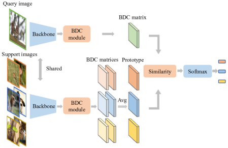
(a) Meta DeepBDC–Instantiation with ProtoNet [33] as a blueprint.

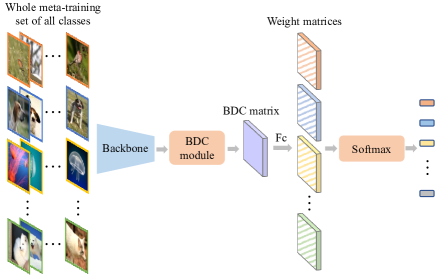
(b) STL DeepBDC–Instantiation based on Good-Embed [37] relying on non-episodic training.

Figure 1: Two instantiations of our DeepBDC for few-shot classification. Meta DeepBDC (a) is based on the idea of meta learning which depends on episodic training; here we take a 3-way 2-shot classification as an example for illustration. In STL DeepBDC (b), we train a network with a conventional softmax classifier and cross-entroy loss on the whole meta-training spanning all classes; during meta-testing, we use the trained network as an embedding model for feature extraction, constructing and training a logistic regression model for classification.

3.3 Instantiating DeepBDC for Few-shot Learning

We instantiate our DeepBDC based on meta-learning framework and on simple transfer learning framework, and the resulting Meta DeepBDC and STL DeepBDC are shown in Fig. 1(a) and Fig. 1(b), respectively.

Meta DeepBDC Standard few-shot learning is performed in an episodic manner on a multitude of tasks. A task is often formulated as a $N$-way $K$-shot classification problem, which spans $N$ classes each with $K$ support images and $Q$ query images, on a support set $\mathcal{D}^{\mathrm{sup}}=\{(\mathbf{z}_{j},y_{j})\}_{j=1}^{NK}$ and a query set $\mathcal{D}^{\mathrm{que}}=\{(\mathbf{z}_{j},y_{j})\}_{j=1}^{NQ}$. A learner is trained on $\mathcal{D}^{\mathrm{sup}}$ and makes predictions on $\mathcal{D}^{\mathrm{que}}$.

We instantiate Meta DeepBDC with ProtoNet [33] as a blue print. It learns a metric space where classification is performed by computing distances to the prototype of every class. On one task $(\mathcal{D}^{\mathrm{sup}},\mathcal{D}^{\mathrm{que}})$, we feed image $\mathbf{z}_{j}$ to the network to produce the BDC matrix $\mathbf{A}_{\boldsymbol{\uptheta}}(\mathbf{z}_{j})$. The prototype of the support class $k$ is the average (Avg) of the BDC matrices belonging to its class:

$$\mathbf{P}_{k}=\frac{1}{K}\sum_{(\mathbf{z}_{j},y_{j})\in\mathcal{S}_{k}}\mathbf{A}_{\boldsymbol{\uptheta}}(\mathbf{z}_{j})$$ (7)

where $\mathcal{S}_{k}$ is the set of examples in $\mathcal{D}^{\mathrm{sup}}$ labeled with class $k$. We produce a distribution over classes based on a softmax over distances to the prototypes of the support classes, and then formulate the following loss function:

$$\!\arg\min_{\boldsymbol{\uptheta}}\;\;-\!\!\!\!\!\!\sum_{(\mathbf{z}_{j},y_{j})\in\mathcal{D}^{\mathrm{que}}}\!\!\log\frac{\exp(\tau\mathrm{tr}(\mathbf{A}_{\boldsymbol{\uptheta}}(\mathbf{z}_{j})^{T}\mathbf{P}_{{y}_{j}}))}{\sum_{k}\exp(\tau\mathrm{tr}(\mathbf{A}_{\boldsymbol{\uptheta}}(\mathbf{z}_{j})^{T}\mathbf{P}_{k}))}$$ (8)

where $\tau$ is a learnable scaling parameter [45, 46, 5].

We train the learner by sampling tasks from a massive meta-training set $\mathcal{C}^{\mathrm{train}}$ where the number of classes is far larger than $N$. Then, we sample tasks from a held-out meta-testing set $\mathcal{C}^{\mathrm{test}}$ on which we evaluate the performance of the learner. The episodic training ensures consistency between meta-training and meta-testing, which is crucial for the meta-learning methods [39, 33].

STL DeepBDC This instantiation is based on a widely used simple transfer learning (STL) framework [10], in which a deep network is trained on a large dataset and is then used as an embedding model to extract features for downstream tasks with few labeled examples.

We train a conventional image classification task on the whole meta-training set $\mathcal{C}^{\mathrm{train}}$ spanning all classes. The cross-entropy loss between prediction and ground-truth labels is used for training a learner from scratch:

$$\!\!\arg\min_{\boldsymbol{\uptheta},\mathbf{W}_{k}}\;\;-\!\!\!\!\!\!\!\!\sum_{(\mathbf{z}_{j},y_{j})\in\mathcal{C}^{\mathrm{train}}}\!\!\!\!\log\frac{\exp(\tau\mathrm{tr}(\mathbf{A}_{\boldsymbol{\uptheta}}(\mathbf{z}_{j})^{T}\mathbf{W}_{{y}_{j}}))}{\sum_{k}\exp(\tau\mathrm{tr}(\mathbf{A}_{\boldsymbol{\uptheta}}(\mathbf{z}_{j})^{T}\mathbf{W}_{k}))}$$ (9)

where $\mathbf{W}_{k}\in\mathbb{R}^{d\times d}$ is the $k$-th weight matrix and $\tau$ is a learnable scaling parameter. For a task $(\mathcal{D}^{\mathrm{sup}},\mathcal{D}^{\mathrm{que}})$ sampled from meta-testing set $\mathcal{C}^{\mathrm{test}}$, we build and train a new linear classifier for $K$ classes on $\mathcal{D}^{\mathrm{sup}}$, using the trained model as a feature extractor. Following [37], we adopt the logistic regression model for classification, and, instead of directly using the trained model for meta-testing tasks, a sequential self-distillation technique is used to distill knowledge from the trained model on the meta-training set.

By referring to Eq. (8) and Eq. (9), we can interpret $\mathbf{W}_{k}$ as the prototype of class $k$, a dummy BDC matrix learned through training. Note that similar interpretations are given in DeepEMD [47] and FRN [45]. It is worth mentioning that, by vectorization operation as described in Eq. (5) for both the BDC matrices and the weight matrices, the softmax function in Eq. (9) can be implemented via a standard fully-connected (FC) layer.

3.4 Relation with Previous Methods

Let $\{\mathbf{x}_{j}\}_{j=1}^{n}$ be features of a query image, viewed as the observations of a random vector $X$. One can compute the mean vector $\boldsymbol{\upmu}_{X}=\frac{1}{n}\sum_{j=1}^{n}\mathbf{x}_{j}$, covariance matrix $\boldsymbol{\Sigma}_{X}=\frac{1}{n}\sum_{j=1}^{n}(\mathbf{x}_{j}-\boldsymbol{\upmu}_{X})(\mathbf{x}_{j}-\boldsymbol{\upmu}_{X})^{T}$ or Gaussian distribution $\mathcal{N}_{\boldsymbol{\mu}_{X},\boldsymbol{\Sigma}_{X}}$, as image representations. Note that these representations have been extensively studied outside of the few-shot learning regime, where they are deemed global average pooling [13], bilinear [22] or covariance pooling [42], and Gaussian pooling [41], respectively. The corresponding prototypes of the support class, $\boldsymbol{\upmu}_{Y}$, $\boldsymbol{\Sigma}_{Y}$ or $\mathcal{N}_{\boldsymbol{\mu}_{Y},\boldsymbol{\Sigma}_{Y}}$, can be computed using the features of $K$ support images.

ProtoNet [33] represents the images with the mean vector and measures the difference using Euclidean distance $\rho_{\mathrm{ProtoNet}}(X,Y)\!\!=\!\!\|\boldsymbol{\upmu}_{X}\!\!-\!\!\boldsymbol{\upmu}_{Y}\|^{2}$ or cosine similarity ${\boldsymbol{\upmu}_{X}^{T}\boldsymbol{\upmu}_{Y}}/(\|\boldsymbol{\upmu}_{X}\|\|\boldsymbol{\upmu}_{Y}\|)$ for metric learning.

CovNet [44] adopts the covariance matrices as image representations for improving the first-order representation. The covariance matrices are subject to signed square-root normalization and then are compared with the Euclidean distance in the matrix space (i.e., the Frobenius norm) $\rho_{\mathrm{CovNet}}(X,Y)=\|\boldsymbol{\Sigma}_{X}-\boldsymbol{\Sigma}_{Y}\|^{2}$.

ADM [20] proposes to use an asymmetric distribution measure (ADM) to evaluate the dis-similarity between the query image and the support class. The distributions of images are represented by multivariate Gaussians whose differences are measured by KL-divergence $\rho_{\mathrm{ADM}}(X,Y)=D_{\mathrm{KL}}(\mathcal{N}_{\boldsymbol{\mu}_{X},\boldsymbol{\Sigma}_{X}}||\mathcal{N}_{\boldsymbol{\mu}_{Y},\boldsymbol{\Sigma}_{Y}})$.

DeepEMD [47] uses discrete distributions as image representations. Specifically, the discrete PDF of the query image is $f_{X}(\mathbf{x})\!\!=\!\!\sum_{j=1}^{n}\!f_{\mathbf{x}_{j}}\delta_{\mathbf{x},\mathbf{x}_{j}}$, where $f_{\mathbf{x}_{j}}$ denotes the probability of $\mathbf{x}_{j}$ and $\delta_{\mathbf{x},\mathbf{x}_{j}}$ is the Kronecker delta which is equal to 1 if $\mathbf{x}\!\!=\!\!\mathbf{x}_{j}$ and zero otherwise. Let the PDF of a support image be $f_{Y}(\mathbf{y})\!\!=\!\!\sum_{j=1}^{n}\!f_{\mathbf{y}_{j}}\delta_{\mathbf{y},\mathbf{y}_{j}}$. The distance between $f_{X}(\mathbf{x})$ and $f_{Y}(\mathbf{y})$ is formulated as EMD, i.e., $\rho_{\mathrm{EMD}}(X,Y)\!\!=\!\!\min_{f_{\mathbf{x}_{j},\mathbf{y}_{l}}\geq 0}\sum_{j=1}^{n}\!\sum_{l=1}^{n}\!f_{\mathbf{x}_{j},\mathbf{y}_{l}}c_{\mathbf{x}_{j},\mathbf{y}_{l}}$ with constraints $\sum_{l=1}^{n}\!f_{\mathbf{x}_{j},\mathbf{y}_{l}}\!\!=\!\!f_{\mathbf{x}_{j}}$ and $\sum_{j=1}^{n}\!f_{\mathbf{x}_{j},\mathbf{y}_{l}}\!\!=\!\!f_{\mathbf{y}_{l}}$ for $j,l\!=\!1,\ldots,n$. Here $c_{\mathbf{x}_{j},\mathbf{y}_{l}}$ is the transport cost. Thus, EMD seeks an optimal joint distribution $f_{XY}(\mathbf{x}_{j},\mathbf{y}_{l})\!\stackrel{{\scriptstyle\scriptscriptstyle\vartriangle}}{{=}}\!f_{\mathbf{x}_{j},\mathbf{y}_{l}}$ such that the expectation of transportation cost is minimal [29, Sec. 2.3]. DeepEMD proposes a cross-reference mechanism to define $f_{\mathbf{x}_{j}}$ and $f_{\mathbf{y}_{l}}$, and a structured FC layer to handle $K$-shot classification ($K$$>$$1$).

$d$ Parameters 1-shot 5-shot (M) Acc Latency Acc Latency 1280 13.25 66.36$\pm$0.43 488 83.23$\pm$0.30 614 960 13.04 66.81$\pm$0.44 280 83.68$\pm$0.28 351 640 12.84 67.34$\pm$0.43 161 84.46$\pm$0.28 198 512 12.75 67.10$\pm$0.45 134 84.23$\pm$0.28 164 256 12.59 66.90$\pm$0.43 121 84.15$\pm$0.28 148 ProtoNet [33] 62.11$\pm$0.44 115 80.77$\pm$0.30 143 Similarity function 1-shot 5-shot Acc Latency Acc Latency Inner product 67.34$\pm$0.43 161 82.38$\pm$0.32 193 Cosine similarity 61.74$\pm$0.42 172 82.49$\pm$0.31 207 Euclidean distance 56.70$\pm$0.45 163 84.46$\pm$0.28 198 (a) Meta DeepBDC based on ProtoNet [33] as a blueprint.

$d$ Parameters 1-shot 5-shot (M) Acc Latency Acc Latency 512 13.41 64.92$\pm$0.43 1110 84.61$\pm$0.29 2016 256 12.75 66.15$\pm$0.43 371 85.44$\pm$0.29 587 196 12.65 66.57$\pm$0.43 285 85.36$\pm$0.29 424 128 12.55 67.83$\pm$0.43 184 85.45$\pm$0.30 245 64 12.48 66.97$\pm$0.44 137 83.18$\pm$0.30 172 Good-Embed [37] 64.82$\pm$0.44 121 82.14$\pm$0.43 155 Classifier 1-shot 5-shot Acc Latency Acc Latency Logistic regression 67.83$\pm$0.43 184 85.45$\pm$0.30 245 SVM 66.29$\pm$0.44 113 84.73$\pm$0.29 144 Softmax 66.30$\pm$0.44 1250 85.20$\pm$0.29 4374 (b) STL DeepBDC based on [37] relying on non-episodic training.

Table 2: Ablation analysis of our two instantiations of DeepBDC with the backbone of ResNet-12 on miniImageNet. We report accuracy and latency (ms) of one meta-testing task for 5-way classification. Latency is measured with a GeForce GTX 1080.

4 Experiments

We first describe briefly the experimental settings. Next, we perform ablation study on our two instantiations (i.e., Meta DeepBDC and STL DeepBDC) and make comparisons to the counterparts. Finally, we compare with state-of-the-art methods on six few-shot datasets, covering general object recognition, fine-grained categorization and cross-domain classification.

Method	1-shot		5-shot
	Acc	Latency	Acc	Latency
ProtoNet [33]	62.11$\pm$0.44	115	80.77$\pm$0.30	143
ADM [20]	65.87$\pm$0.43	199	82.05$\pm$0.29	221
CovNet [44]	64.59$\pm$0.45	120	82.02$\pm$0.29	144
DeepEMD [47]	65.91$\pm$0.82	457	82.41$\pm$0.56	12617
Meta DeepBDC	67.34$\pm$0.43	161	84.46$\pm$0.28	198
STL DeepBDC	67.83$\pm$0.43	184	85.45$\pm$0.29	245

Table 3: Comparison of accuracy and latency (ms) of 5-way classification to the counterparts with the backbone of ResNet-12 on miniImageNet.

4.1 Experimental Settings

Datasets We experiment on two general object recognition benchmarks, i.e., miniImageNet [39] and tieredImageNet [31], and one fine-grained image classification dataset, i.e., CUB-200-2011 [40] (CUB for short). We also evaluate domain transfer ability of models by training on miniImageNet and then test on CUB [40], Aircraft [24] and Cars [16].

Backbone network For fair comparisons with previous methods, we use two kinds of networks as backbones, i.e., ResNet-12 [37, 18] and ResNet-18 [1, 23, 34]. Same as commonly used practice, the input resolution of images is 84$\times$84 for ResNet-12 and 224$\times$224 for ResNet-18, respectively. Moreover, we adopt deeper models with higher capacity, i.e., ResNet-34 [13] with input images of 224$\times$224 and a variant of ResNet-34 fit for input images of 84$\times$84. Similar to [9, 20], we remove the last down-sampling of backbones to obtain more convolutional features.

Training Our Meta DeepBDC is based on meta-learning framework, depending on episodic training. Each episode (task) concerns standard 5-way 1-shot or 5-way 5-shot classification, uniformly sampled from meta-training or meta-testing set; following [47, 45, 5], before episodic training, we pre-train the models whose weights are used as initialization. Contrary to Meta DeepBDC, our STL DeepBDC is based on simple transfer learning framework, requiring non-episodic training. Following [37], we train a network as an embedding model with cross-entropy loss on the whole meta-training set spanning all classes; for each meta-testing task, we train a new logistic regression classifier using the features extracted by the embedding model.

In supplement (Supp.) S1, we provide statistics of datasets and the splits of meta training/validation/test sets, as well as details on network architectures, optimizers, hyperparameters, etc.

4.2 Ablation Study

Method Backbone miniImageNet tieredImageNet 1-shot 5-shot 1-shot 5-shot CTM [19] ResNet-18 64.12$\pm$0.82 80.51$\pm$0.13 68.41$\pm$0.39 84.28$\pm$1.73 S2M2 [25] ResNet-18 64.06$\pm$0.18 80.58$\pm$0.12 – – TADAM [26] ResNet-12 58.50$\pm$0.30 76.70$\pm$0.38 – – MetaOptNet [18] ResNet-12 62.64$\pm$0.44 78.63$\pm$0.46 65.99$\pm$0.72 81.56$\pm$0.63 DN4 [21] † ResNet-12 64.73$\pm$0.44 79.85$\pm$0.31 – – Baseline++ [4] † ResNet-12 60.56$\pm$0.45 77.40$\pm$0.34 – – Good-Embed[37] ResNet-12 64.82$\pm$0.60 82.14$\pm$0.43 71.52$\pm$0.69 86.03$\pm$0.58 FEAT  [46] ResNet-12 66.78$\pm$0.20 82.05$\pm$0.14 70.80$\pm$0.23 84.79$\pm$0.16 Meta-Baseline [5] ResNet-12 63.17$\pm$0.23 79.26$\pm$ 0.17 68.62$\pm$0.27 83.29$\pm$0.18 MELR [11] ResNet-12 67.40$\pm$0.43 83.40$\pm$0.28 72.14$\pm$0.51 87.01$\pm$0.35 FRN [45] ResNet-12 66.45$\pm$0.19 82.83$\pm$0.13 71.16$\pm$0.22 86.01$\pm$0.15 IEPT [50] ResNet-12 67.05$\pm$0.44 82.90$\pm$0.30 72.24$\pm$0.50 86.73$\pm$0.34 BML [51] ResNet-12 67.04$\pm$0.63 83.63$\pm$0.29 68.99$\pm$0.50 85.49$\pm$0.34 ProtoNet [33] † ResNet-12 62.11$\pm$0.44 80.77$\pm$0.30 68.31$\pm$0.51 83.85$\pm$0.36 ADM [20] † ResNet-12 65.87$\pm$0.43 82.05$\pm$0.29 70.78$\pm$0.52 85.70$\pm$0.43 CovNet [44] † ResNet-12 64.59$\pm$0.45 82.02$\pm$0.29 69.75$\pm$0.52 84.21$\pm$0.26 DeepEMD [47] ResNet-12 65.91$\pm$0.82 82.41$\pm$0.56 71.16$\pm$0.87 86.03$\pm$0.58 Meta DeepBDC ResNet-12 67.34$\pm$0.43 84.46$\pm$0.28 72.34$\pm$0.49 87.31$\pm$0.32 STL DeepBDC ResNet-12 67.83$\pm$0.43 85.45$\pm$0.29 73.82$\pm$0.47 89.00$\pm$0.30 (a) Results on general object recognition datasets.

Method Backbone CUB 1-shot 5-shot ProtoNet [33] Conv4 64.42$\pm$0.48 81.82$\pm$0.35 FEAT [46] Conv4 68.87$\pm$0.22 82.90$\pm$0.15 MELR [11] Conv4 70.26$\pm$0.50 85.01$\pm$0.32 MVT [27] ResNet-10 – 85.35$\pm$0.55 MatchNet [39] ResNet-12 71.87$\pm$0.85 85.08$\pm$0.57 Wang et al. LR [43] ResNet-12 76.16 90.32 MAML [12] ResNet-18 68.42$\pm$1.07 83.47$\pm$0.62 $\Delta$-encoder [32] ResNet-18 69.80 82.60 Baseline++ [4] ResNet-18 67.02$\pm$0.90 83.58$\pm$0.54 AA [1] ResNet-18 74.22$\pm$1.09 88.65$\pm$0.55 Neg-Cosine [23] ResNet-18 72.66$\pm$0.85 89.40$\pm$0.43 LaplacianShot [52] ResNet-18 80.96 88.68 FRN [45] † ResNet-18 82.55$\pm$0.19 92.98$\pm$0.10 Good-Embed[37] † ResNet-18 77.92$\pm$0.46 89.94$\pm$0.26 ProtoNet [33] † ResNet-18 80.90$\pm$0.43 89.81$\pm$0.23 ADM [20] † ResNet-18 79.31$\pm$0.43 90.69$\pm$0.21 CovNet [44] † ResNet-18 80.76$\pm$0.42 92.05$\pm$0.20 Meta DeepBDC ResNet-18 83.55$\pm$0.40 93.82$\pm$0.17 STL DeepBDC ResNet-18 84.01$\pm$0.42 94.02$\pm$0.24 (b) Results on fine-grained categorization dataset.

Table 4: Comparison with state-of-the-art methods for both general and fine-grained few-shot image classification. The best results are in bold black and second-best ones are in red. ^† Reproduced with our setting.

We perform ablation analysis of our two instantiations and compare to the counterparts on miniImageNet for 5-way task, with ResNet-12 as the backbone. Additional details on implementation of the counterparts and extra experiments are respectively given in Supp. S-2 and Supp. S-3.

Ablation analysis of Meta DeepBDC As the sizes of BDC matrices are quadratic in the number of channels, we introduce a $1$$\times$$1$ convolution (conv) layer, decreasing the channel number to $d$. In our implementation, each BDC matrix is vectorized as in Eq. (5), thus is of size $d(d+1)/2$. Tab. 2(a) (top) shows the effect of varying $d$ on accuracy and on meta-testing time per episode. We can see that the highest accuracy is achieved when $d\!=\!640$; meanwhile, the meta-testing time only increases moderately as $d$ enlarges. We also experiment by directly attaching BDC module to the backbone without the additional $1\!\times\!1$ conv layer; we achieve 67.10$\pm$0.43 and 84.50$\pm$0.28 for 1-shot and 5-shot, respectively, comparable to the best result obtained by using the additional $1\!\times\!1$ conv layer. Besides the inner product as depicted in Eq. (5), we can also use Euclidean distance or cosine similarity as metric, and the corresponding results are given in Tab. 2(a) (bottom). It can be seen that the inner product performs best for 1-shot task, while the Euclidean distance achieves the highest accuracy for 5-shot. The optimal setting achieved here is used throughout the remaining paper. Finally, we note that Meta DeepBDC has much better performance than the baseline (i.e., ProtoNet), regardless of the value of $d$, while increase of latency is small.

Ablation analysis of STL DeepBDC For each meta-testing task of STL DeepBDC, we need to build and train a new linear classifier which introduces parameters and computations. As the size of BDC matrix is quadratic in $d$, the number of parameters is considerable relative to that of training examples, particularly for larger $d$. Therefore, with increase of $d$, there exist greater risk of overfitting, which may explain why overall the accuracy becomes lower when $d$ is larger for both 1-shot and 5-shot tasks, as shown in Tab. 2(b) (top). STL DeepBDC with $d\!=\!128$ obtains the best result, higher than the best result of Meta DeepBDC while taking comparable time. Besides the logistic regression model, we compare with softmax classifier and linear SVM as well. From the results in Tab. 2(b) (bottom), we can see that the softmax classifier is on par with SVM, while both of them are inferior to the logistic regression; the latency of logistic regression is larger than SVM while the softmax classifier takes remarkably larger time than the other two. At last, we mention that STL DeepBDC with $d\!=\!128$ outperforms the baseline of Good-Embed by a large margin with moderate increase of latency.

The i.i.d. assumption underlying DeepBDC The BDC metric depends on the i.i.d. assumption [35] which is common in statistics and machine learning. As in Sec. 3.2, by viewing each channel (feature map) as a random observation, we obtain $d\!\times\!d$ matrices corresponding to the spatial pooling. Alternatively, one can regard each spatial feature as a random observation, leading to $hw\!\times\!hw$ matrices which correspond to a channel pooling; however, for 1-shot/5-shot task and with the same setting as in Tab. 2(a), this produces $62.55$$\pm$$0.45$/$78.88$$\pm$$0.32$ and $63.95$$\pm$$0.45$/$79.45$$\pm$$0.32$ for Meta DeepBDC ($d\!=\!640$) and STL DeepBDC ($d\!=\!128$), respectively, much lower than the accuracies of spatial pooling. Note that the i.i.d. assumption may not hold for either spatial or channel pooling; our comparison suggests the spatial pooling is a better option.

Comparison to the counterparts Here we compare with the counterparts whose representations are based on distribution modeling. Like our DeepBDC, both ADM and CovNet need to estimate second moments, which leads to quadratic increase of representations. Therefore, for a fair comparison with them, we also add a $1$$\times$$1$ convolution with $d$ channels for dimension reduction, obtaining the best results for them by tuning $d$. The comparion results are presented in Tab. 3.

Method Backbone 5-shot Baseline [4] ResNet-18 65.57$\pm$0.70 Baseline++ [4] ResNet-18 62.04$\pm$0.76 GNN+FT [38] ResNet-12 66.98$\pm$0.68 BML [51] ResNet-12 72.42$\pm$0.54 FRN [45] ResNet-12 77.09$\pm$0.15 ProtoNet [33] † ResNet-12 67.19$\pm$0.38 Good-Embed [37] † ResNet-12 67.43$\pm$0.44 ADM [20] † ResNet-12 70.55$\pm$0.43 CovNet [44] † ResNet-12 76.77$\pm$0.34 Meta DeepBDC ResNet-12 77.87$\pm$0.33 STL DeepBDC ResNet-12 80.16$\pm$0.38 (a) miniImageNet $\rightarrow$ CUB.

Method Backbone 5-shot ProtoNet [33] † ResNet-12 55.96$\pm$0.38 ADM [20] † ResNet-12 65.40$\pm$0.36 CovNet [44] † ResNet-12 63.56$\pm$0.37 Baseline [4] † ResNet-12 59.04$\pm$0.36 Baseline++ [4] † ResNet-12 56.50$\pm$0.38 Good-Embed [37] † ResNet-12 58.95$\pm$0.38 Meta DeepBDC ResNet-12 68.67$\pm$0.39 STL DeepBDC ResNet-12 69.07$\pm$0.39 (b) miniImageNet $\rightarrow$ Aircraft.

Method Backbone 5-shot ProtoNet [33] † ResNet-12 46.30$\pm$0.36 ADM [20] † ResNet-12 53.94$\pm$0.35 CovNet [44] † ResNet-12 52.90$\pm$0.37 Baseline [4] † ResNet-12 50.29$\pm$0.37 Baseline++ [4] † ResNet-12 46.44$\pm$0.37 Good-Embed [37] † ResNet-12 50.18$\pm$0.37 Meta DeepBDC ResNet-12 54.61$\pm$0.37 STL DeepBDC ResNet-12 58.09$\pm$0.36 (c) miniImageNet $\rightarrow$ Cars.

Table 5: Comparison with state-of-the-art methods for 5-way 5-shot classification in cross-domain scenarios. The best results are in bold black and second-best ones are in red. ^† Reproduced with our setting.

Regarding the accuracy, we have several observations. (1) ProtoNet is inferior to CovNet and ADM, suggesting that second moments have better capability to model marginal distributions than first moment. (2) DeepEMD outperforms CovNet and ADM, which indicates that joint distribution modeling via EMD is superior to modeling of marginal distributions. (3) Both our two instantiations outperform the counterparts by large margins. We attribute this to that BDC has stronger capability of statistical dependency modeling by effectively harnessing joint distributions. As to the latency, our two instantiations both take a little longer time than ProtoNet and CovNet, while being comparable to ADM. Notably, DeepEMD is computationally expensive, $\sim$ 2 times and 50 times slower than the other methods for 1-shot and 5-shot tasks, respectively.

4.3 Comparison with State-of-the-art Methods

General object recognition According to Tab. 4(a), on miniImageNet, for 1-shot task Meta DeepBDC is on par with state-of-the-art MELR while STL DeepBDC is better than it; for 5-shot task, Meta DeepBDC and STL DeepBDC outperform BML, which previously achieved the best result, by 0.83 percentage points (abbreviated as pp hereafter) and 1.82 pp, respectively. Our Meta DeepBDC can be further improved by combining Image-to-Class Measure (DN4) following the idea introduced in [20]; accordingly, we achieve 67.86$\pm$0.41/85.14$\pm$0.29 for 1-shot/5-shot tasks, outperforming ADM+DN4 (66.53$\pm$0.43/82.61$\pm$0.30). On tieredImageNet, for 1-shot task Meta DeepBDC is slightly better than state-of-the-art IEPT while STL DeepBDC outperforms it by 1.58 pp; for 5-shot task, Meta DeepBDC achieves slight gains (0.3 pp) over state-of-the-art MELR while STL DeepBDC has much larger gains ($\sim$2.0 pp).

Fine-grained categorization Following [4, 23, 1], we conduct experiments on CUB with the original raw images. We reproduce ProtoNet and Good-Embed which are our baselines as well as FRN. From Tab. 4(b), we can see that reproduced ProtoNet and Good-Embed are competitive with previous published accuracies, indicating our re-implemented baselines provide fair competition; moreover, our methods are high-ranking across the board, compared to state-of-the-art FRN, the gains of Meta DeepBDC and STL DeepBDC are 1.0/1.5 pp and 0.8/1.0 pp for 1-shot/5-shot task, respectively. Furthermore, by adopting ResNet-34 with 224$\times$224 input images, our methods further improve. Specifically, Meta DeepBDC and STL DeepBDC achieve 85.25$\pm$0.39/94.31$\pm$0.17 and 84.69$\pm$0.43/94.33$\pm$0.21, respectively, outperforming corresponding baselines of ProtoNet (80.58$\pm$/90.11$\pm$0.26) and Good-Embed (79.33$\pm$0.48/90.10$\pm$0.28).

Cross-domain classification Finally, we evaluate 5-way 5-shot classification in cross-domain scenarios, by training on miniImageNet and testing on three widely used fine-grained datasets. Except DeepEMD which is computationally prohibitive for us, we implement all counterparts based on distribution modeling, and Good-Embed on the three datasets, as well as Baseline and Baseline++ [4] on Aircraft and Cars. The results are shown in Tab. 5. On miniImageNet$\rightarrow$CUB, CovNet is very competitive, only slightly inferior to FRN, and both of them are much better than the other methods except ours. Meta DeepBDC and STL DeepBDC outperform the high-performing FRN by 0.8 pp and 3.1 pp, respectively. On miniImageNet$\rightarrow$Aircraft, our two instantiations improve over all the other compared methods by more than 3.2 pp. On miniImageNet$\rightarrow$Cars, ADM is superior among our competitors; compared to it, Meta DeepBDC and STL DeepBDC achieve 0.7 pp and 4.2 pp higher accuracies, respectively. These comparisons demonstrate that our models have stronger domain transfer capability.

5 Conclusion

In this paper, we propose a deep Brownian Distance Covariance (DeepBDC) method for few-shot classification. DeepBDC can effectively learn image representations by measuring, for the query and support images, the discrepancy between the joint distribution of their embedded features and product of the marginals. The core of DeepBDC is formulated as a modular and efficient layer, which can be flexibly inserted into deep networks, suitable not only for meta-learning framework based on episodic training, but also for the simple transfer learning framework that relies on non-episodic training. Extensive experiments have shown that our DeepBDC method performs much better than the counterparts, and furthermore, sets new state-of-the-art results on multiple general, fine-grained and cross-domain few-shot classification tasks. Our work shows great potential of BDC, a fundamental but overlooked technique, and encourages its future applications in deep learning.

Supplementary Material

In this supplement, we present details on the implementations of our DeepBDC and the counterparts. Besides, we conduct experiments providing additional ablation study and comparison. We finally show BDC’s ability to characterize non-linear dependence.

S1  Implementations

S1-1  Benchmarks

miniImageNet The miniImageNet [S-22] is a few-shot benchmark constructed from ImageNet [S-6] for general object recognition. It consists of 100 classes each of which contains 600 images. Following previous works [S-4, S-25, S-26], we use the splits provided by [S-18], which involves 64 classes for meta-training, 16 classes for meta-validation and the remaining 20 classes for meta-testing.

tieredImageNet The tieredImageNet [S-19] is also a few-shot benchmark for general object recognition. It is constructed from ImageNet [S-6] as well, which, different from miniImageNet, considers the hierarchical structure of ImageNet. This dataset contains 608 classes from 34 super-classes and a total of 779,165 images. Among these classes, 20 super-classes (351 classes) are used for meta-training, 6 super-classes (97 classes) for meta-validation and the remaining 8 super-classes (160 classes) for meta-testing.

CUB Caltech-UCSD Birds-200-2011 [S-23] (CUB) dataset is a widely used fine-grained categorization benchmark. This dataset contains 200 bird classes with 11,788 images in total. We use the splits of  [S-4], in which the total classes are divided into 100/50/50 for meta-training/validation/testing. Following [S-4, S-14, S-1], we conduct experiments on CUB with the original raw images, instead of cropped images via annotated bounding boxes [S-26, S-27].

miniImageNet $\rightarrow$ CUB Chen et al. [S-4] build the cross-domain task for assessing the domain transfer ability of the models. In this setting, all 100 classes of miniImageNet are used for meta-training, while the models are evaluated on the meta-testing set (50 classes) of CUB.

miniImageNet $\rightarrow$ Aircraft Aircraft [S-15] contains 10,000 images from 100 classes. We perform meta-training on the whole miniImageNet; we adopt the splits on Aircraft proposed by [S-25], where 25 classes are used for meta-validation and 25 classes are for meta-testing. Same as [S-25], we conduct experiments with the images cropped by using the bounding box annotations.

miniImageNet $\rightarrow$ Cars Stanford Cars [S-10] (Cars) contains 196 classes and a total 16,185 images. We follow the splits of [S-13] to build the meta-validation set (17 classes) and meta-testing set (49 classes). Similar to the other cross-domain benchmarks, the full miniImageNet is used as meta-training set.

Method	Hyper-params	miniImageNet	tieredImageNet	CUB	miniImageNet $\rightarrow$ CUB$/$Aircraft$/$Cars
Meta DeepBDC	Initial LR	1e-4	5e-5	1e-3	5e-5
	LR decay	[40, 80]*0.1	[70]*0.1	[40, 80]*0.1	[70]*0.1
	Epochs	100	100	100	100
STL DeepBDC	Initial LR	5e-2	5e-2	5e-2	5e-2
	LR decay	[100,150]*0.1	[40,70]*0.1	[120,170]*0.1	[100,150]*0.1
	Epochs	180	100	220	180

Table S-1: Hyperparameter settings of our DeepBDC.

S1-2  Architectures

For fair comparisons with previous methods, we use two kinds of networks as backbones, i.e., ResNet-12 and ResNet-18. Following previous practice, the input resolution of images is $84\!\times\!84$ for ResNet-12, and $224\!\times\!224$ for ResNet-18, respectively. Besides, we use higher capacity models, i.e., ResNet-34 with input images of $224\!\times\!224$ and its variant fit for input images of 84$\times$84.

As in [S-21, S-11, S-16, S-25], ResNet-12 consists of four stages each of which contains one residual block. The widths of the residual blocks of the four stages are [64, 160, 320, 640]. Each residual block has three 3$\times$3 convolution layers with a batch normalization and a 0.1 leaky ReLU. Right after every block except the last one, a 2$\times$2 max pooling layer is used to down-sample the feature maps. We adopt ResNet-18 and ResNet-34 proposed in [S-8] with the last down-sampling being removed. The architecture of the variant of ResNet-34 is same as that of ResNet-12, except that the numbers of residual blocks of the four stages are [2, 3, 4, 2], instead of [1, 1, 1, 1] in ResNet-12.

S1-3  Training and Evaluation Protocols

Training

During training, following [S-4, S-25, S-27], we use standard data augmentation including random resized crop, color jittering and random horizontal flip on all benchmarks. We adopt the SGD algorithm with a momentum of 0.9 and a weight decay of 5e-4 to train our proposed DeepBDC networks. For ResNet-12, we apply DropBlock [S-7] regularization during training as in [S-26, S-11, S-5]. We tune the number of epochs and the scheduling of learning rate (LR) on different benchmarks.

For our Meta DeepBDC which is based on meta-learning framework, we train the model by uniformly sampling episodes (tasks) from the meta-training set. Following previous works [S-5, S-25, S-27], right before performing the episodic training, we pre-train the networks on the full meta-training set whose weights are used as initialization. To sample a 5-way 1-shot task, we randomly pick up 5 classes each with 1 support image and 16 query images selected at random. Similarly, every 5-way 5-shot task contains 5 support images and 16 query images. Tab. S-1 (upper part) shows the hyper-parameter settings for training Meta DeepBDC on all benchmarks. Let us take miniImageNet as an example: the initial learning rate (LR) is 1e-4, which is divided by 10 at epoch 40 and 80, respectively, and training proceeds until epoch 100. We adopt the model achieving highest accuracy on the meta-validation for evaluation on the meta-testing set.

Our STL DeepBDC is based on Good-Embed [S-21], which falls into simple transfer learning framework, not requiring episodic training. In practice, we train the network for a common multi-way classification task, using a soft-max classifier via a standard cross-entropy loss on the whole meta-training set spanning all classes. We set the batch size to 64 across all benchmarks. Furthermore, following [S-21], we conduct sequential self-distillation to distill knowledge from the trained model. The networks thus obtained are used as embedding models for extracting features (i.e., outputs of the last convolution layer of one network). The hyper-parameter settings for STL DeepBDC are shown in Tab. S-1 (bottom part).

Evaluation

We uniformly sample episodes (tasks) from the meta-testing set to evaluate the models’ performance. Following  [S-4], we build 5-way 1-shot or 5-shot setting, respectively, both with 15 query images. We report mean accuracy of 2,000 episodes with 95% confidence intervals. Our Meta DeepBDC does not require additional training, so we directly performing testing. Our STL DeepBDC needs to train a linear classifier for each episode using the trained model for feature extraction. We implement the logistic regression via L-BFGS-B algorithm and linear SVM via LIBSVM based on scikit-learn software package [S-17]. We perform L2 normalization for the features in logistic regression and SVM; furthermore, we standardize the normalized features before fed to SVM. Implementation of the soft-max classifier is based on PyTorch, where we adopt SGD algorithm with a batch size of 4, a momentum of 0.9, a weight decay of 1e-3 and a learning rate of 1e-2.

S2  Implementation of the Counterparts

ProtoNet We use implementation of Chen et al. [S-4] which is public available .

ADM We use the code released by the authors [S-12] . Differently, we add one 1$\times$1 convolution for dimension reduction before computing mean vectors and covariance matrices. As the original method performs unsatisfactorily, we use a different one fusing ADM and DN4 [S-13]. Specifically, we attach independently the ADM branch and DN4 branch to the backbone, both with individually learnable scaling parameters. Next, the negative KL-divergence score and Image-to-Class (I2C) score are separately fed to softmax and are then added for the final cross entropy loss. We combine Meta DeepBDC and DN4 similarly.

CovNet We mainly follow implementation of the authors  [S-24] . Practically, we have two differences: (1) we introduce a 1$\times$1 convolution for dimension reduction, and (2) for 5-way 1-shot classification, we use the inner product as the metric, rather than the Frobenious norm which produces poor results.

For all of the aforementioned methods, we remove the last down-sampling of the backbones. Following the previous practice  [S-25, S-5, S-28], we employ the weights of pre-trained models as initialization before performing episodic training.

S3  Additional Experiments

This section introduces additional experiments to ablate our DeepBDC and to compare with the counterparts.

S3-1  On prototype in Meta DeepBDC

In Meta DeepBDC, for the 5-shot setting, the prototype of a support class is computed as the average of BDC matrices of 5 support images belonging to this class. Here, we evaluate two other options for computing the prototype. (1) We average features of 5 support images, and then the averaged features are used to compute the BDC matrix as the prototype. (2) We concatenate features of 5 support images for computing the BDC matrix as the prototype. These two methods achieve accuracies (%) of 82.36 and 83.74 on miniImageNet, respectively, which are lower than the accuracy obtained by averaging 5 support BDC matrices (84.46).

Method	ProtoNet†		Good-Embed†		Meta DeepBDC		STL DeepBDC
	1-shot	5-shot	1-shot	5-shot	1-shot	5-shot	1-shot	5-shot
ResNet-12	62.11	80.77	64.98	82.10	67.34	84.46	67.83	85.45
ResNet-34	64.56	81.16	66.14	82.39	68.20	84.97	68.66	85.47
$\Delta$	2.45	0.39	1.16	0.29	0.86	0.51	0.83	0.02

Table S-2: Comparison of different capacity models on miniImageNet with input images of 84$\times$84. The ResNet-34 model is a variant of [S-8] which is described in Sec. S1-2. ^† Reproduced with our setting.

Method	ProtoNet†		Good-Embed†		Meta DeepBDC		STL DeepBDC
	1-shot	5-shot	1-shot	5-shot	1-shot	5-shot	1-shot	5-shot
ResNet-18	80.90	89.81	77.92	89.94	83.55	93.82	84.01	94.02
ResNet-34	80.58	90.11	79.33	90.10	85.25	94.31	84.69	94.33
$\Delta$	-0.32	0.30	1.41	0.16	1.70	0.49	0.68	0.31

Table S-3: Comparsion of different capacity models on CUB with input images of 224$\times$224. Here we use ResNet-34 proposed in [S-8]. ^† Reproduced with our setting.

S3-2  Effect of Higher Capacity Models

To evaluate the effect of higher capacity models, we conduct experiments on CUB using the ResNet-34 with 224$\times$224 input images, and on miniImageNet using the variant of ResNet-34 with input images of 84$\times$84. We compare our Meta DeepBDC and STL DeepBDC with their respective baselines, i.e., ProtoNet and Good-Embed.

The comparison on miniImageNet is shown in Tab. S-2. It can be seen that, for every method with either setting, the accuracy obtained by using high-capacity ResNet-34 is higher than that using ResNet-12. Among them, the improvements of ProtoNet and Good-Embed for 1-shot task are significant (over 1 percentage points). Despite the improvements, our Meta DeepBDC and STL DeepBDC outperform their corresponding baselines by large margins. According to Tab. S-3 which presents results on CUB, we can see that overall all methods improve when using higher-capacity ResNet-34, while the improvements of ProtoNet are not significant. Again, we observe that our methods are significantly superior to their baselines.

S3-3  Effect of Feature Number on DeepBDC

To obtain more convolutional features, CTX [S-3] removes the last down-sampling in the backbone networks, while ADM [S-12] removes the last two. Similar to them, we also remove down-sampling. On miniImageNet, we evaluate the effect of down-sampling on our DeepBDC. As the input resolution is $84\times 84$ for ResNet-12, the spatial size of feature maps outputted by the original backbone is $5\times 5$ and thus we have a total of 25 features; the spatial sizes become $10\times 10$ and $21\times 21$ if the last down-sampling and the last two are eliminated, respectively.

Tab. S-4 summarize the results. We first notice that variation of feature number has minor effect on our STL DeepBDC for either 1-shot or 5-shot task. Regarding our Meta DeepBDC, it can be seen that for both 1-shot and 5-shot tasks, the accuracy increases slightly when the number of features is 100, but then decreases when provided with 441 features. At last, we note that ProtoNet and Good-Embed achieves individual best results when the feature number is 100 and 25, respectively. Throughout the main paper, we report results with removal of the last down-sampling.

Method	5$\times$5		10$\times$10		21$\times$21
	1-shot	5-shot	1-shot	5-shot	1-shot	5-shot
ProtoNet [S-20] †	61.81	79.62	62.11	80.77	61.45	80.00
Good-Embed [S-21] †	65.73	83.08	64.98	82.10	64.68	81.85
Meta DeepBDC	66.74	83.83	67.34	84.46	66.83	84.20
STL DeepBDC	67.76	85.39	67.83	85.45	67.44	85.44

Table S-4: Accuracy (%) against number of features on miniImageNet for 5-way classification. ^† Reproduced with our setting.

Method	Meta-training		Meta-testing		Accuracy
	1-shot	5-shot	1-shot	5-shot	1-shot	5-shot
ProtoNet [S-20] †	304	365	115	143	62.11	80.77
ADM [S-12] †	908	967	199	221	65.87	82.05
CovNet [S-24] †	310	374	120	144	64.59	82.02
DeepEMD [S-27]	$>$80K	$>$$10^{6}$	457	12,617	65.91	82.41
Meta DeepBDC	505	623	161	198	67.34	84.46
STL DeepBDC	–		184	245	67.83	85.45

Table S-5: Comparison of latency (ms) for 5-way classification on miniImageNet. ^† Reproduced with our setting.

S3-4  Comparison of Latency of Meta-training Task

In the main paper, we compare the latency of meta-testing task. Here, we give additional comparison for meta-training task, which is also important in practice. The latency is measured on miniImageNet with the backbone of ResNet-12. Following the setting of DeepEMD [S-27], we adopt QPTH solver [S-2] in meta-training and OpenCV solver in meta-testing, using the code released by the  authors.

Tab. S-5 shows comparison results for 5-way classification; for reference, we also include latency of meta-testing task and recognition accuracies which have been discussed in the primary paper. As regards the meta-training, we find that ProtoNet and CovNet are fastest, while our Meta DeepBDC is somewhat slower than them. Though the meta-testing speed of ADM is comparable to that of our method, its meta-training latency is much larger than ours; the reason is that backpropagation of ADM involves GPU-unfriendly matrix inversions. Notably, DeepEMD is at least 80 times slower for 1-shot and 1000 times slower for 5-shot than the other methods; we mention that FRN also observes the big latency of DeepEMD [S-25].

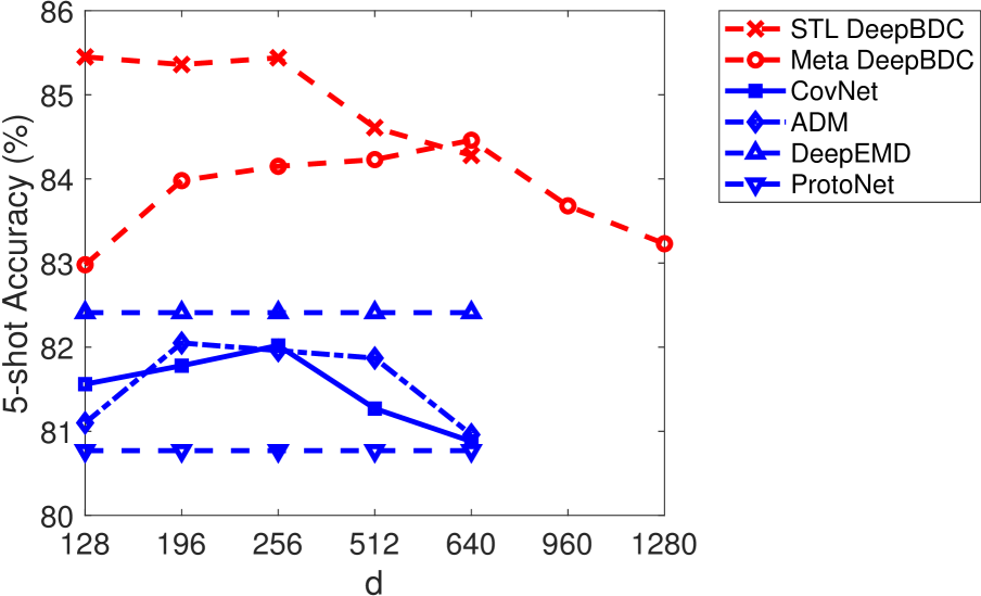
Figure S-1: Accuracy as a function of channel number $d$ for 5-way 5-shot classification on miniImageNet.

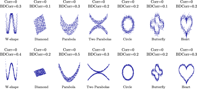
(a) Non-linear relations.

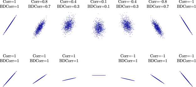
(b) Linear relations.

Figure S-2: Comparison of non-linear (a) and linear (b) relation modeling between classical Correlation ($\mathrm{Corr}$) and Brownian Distance Correlation ($\mathrm{BDCorr}$). This illustration was inspired by D. Boigelot.

S3-5  Effect of Channel Number on DeepBDC and the Counterparts

As described in the main paper, both of CovNet and ADM need to estimate second moments, leading to quadratic increase of representations in channel number $d$. Therefore, for fair comparison, we also add a $1\times 1$ convolution for them to reduce the number of channels. Dimension reduction is hurtful for ProtoNet and DeepEMD, so for them we leave the original channel as it is.

Fig. S-1 plots the curves of accuracies as a function of $d$. In light of the curves, we can draw several conclusions as follows. (1) The channel number $d$ has non-trivial effect on ADM and CovNet. The accuracies (%) of ADM and CovNet reach the highest values when $d=196$ (82.05) and $d=256$ (82.02), respectively. Their accuracies drop gradually when $d$ becomes larger, and when $d=640$, they achieve accuracies only slightly higher than ProtoNet. (2) Across all values of $d$, both instantiations of our DeepBDC clearly perform better than the competing methods.

We mention that our re-implementation non-trivially improves performance of CovNet and ADM, providing fair and competitive baselines. Besides, these results show that dimension reduction plays an important role for second moment-based methods.

S4  Linear and Non-linear Relation Modeling

One of the favorable properties of Brownian Distance Covariance (BDC) is the ability to model both linear and non-linear dependency between random variables $X$ and $Y$. In contrast, traditional covariance can only model linear relations. To facilitate visual understanding, we consider five simulated examples of bivariate distributions [S-9], i.e., “W-shape”, “Diamond”, “Parabola”, “Two parabolas” and “Circle”, and two examples we developed, i.e., “Butterfly” and “Heart”, respectively. In these examples, two random variables $X$ and $Y$ have different kinds of non-linear relationships. Also, we simulate seven kinds of linear relations based on HHG package . For each set of observation pairs, we compute the classical correlation

$$\mathrm{Corr}(X,Y)=\dfrac{\mathrm{cov}(X,Y)}{\sqrt{\mathrm{cov}(X,X)}\sqrt{\mathrm{cov}(Y,Y)}}$$ (S-1)

and Brownian distance correlation

$$\mathrm{BDCorr}(X,Y)=\dfrac{\mathrm{BDC}(X,Y)}{\sqrt{\mathrm{BDC}(X,X)}\sqrt{\mathrm{BDC}(Y,Y)}}$$ (S-2)

Here $\mathrm{cov}(X,Y)$ and $\mathrm{BDC}(X,Y)$ respectively denote the covariance and Brownian distance covariance. Naturally, $\mathrm{cov}(X,X)$ and $\mathrm{BDC}(X,X)$ denote variance and Brownian distance variance of $X$, respectively.

Fig. S-2 shows the scatter plots of the simulated examples together with the values of correlation and Brownian distance correlation. From Fig. 2(a), we can see that for all non-linear relations $\mathrm{Corr}(X,Y)=0$, indicating that classical correlation fails to model such complex relations; on the contrary, Brownian distance correlation can characterize the non-linear dependencies. As shown in Fig. 2(b), compared to correlation, Brownian distance correlation has similar capability to model linear relations, except that it cannot distinguish the orientation as it is always non-negative; besides, both of them cannot reflect the slope of linear relations.

References

- [1] Arman Afrasiyabi, Jean-François Lalonde, and Christian Gagné. Associative alignment for few-shot image classification. In ECCV, 2020.
- [2] Mohamed Ishmael Belghazi, Aristide Baratin, Sai Rajeshwar, Sherjil Ozair, Yoshua Bengio, Aaron Courville, and Devon Hjelm. Mutual information neural estimation. In ICML, 2018.
- [3] Christopher Bishop. Pattern Recognition and Machine Learning. Springer, 2006.
- [4] Wei-Yu Chen, Yen-Cheng Liu, Zsolt Kira, Yu-Chiang Frank Wang, and Jia-Bin Huang. A closer look at few-shot classification. In ICLR, 2019.
- [5] Yinbo Chen, Zhuang Liu, Huijuan Xu, Trevor Darrell, and Xiaolong Wang. Meta-baseline: Exploring simple meta-learning for few-shot learning. In CVPR, 2021.
- [6] Thomas M. Cover and Joy A. Thomas. Elements of information theory. John Wiley & Sons, 2005.
- [7] Benjamin Cowley, Joao Semedo, Amin Zandvakili, Matthew Smith, Adam Kohn, and Byron Yu. Distance Covariance Analysis. In AISTATS, pages 242–251, 2017.
- [8] Guneet S. Dhillon, Pratik Chaudhari, Avinash Ravichandran, and Stefano Soatto. A baseline for few-shot image classification. In ICLR, 2020.
- [9] Carl Doersch, Ankush Gupta, and Andrew Zisserman. Crosstransformers: spatially-aware few-shot transfer. In NIPS, 2020.
- [10] Jeff Donahue, Yangqing Jia, Oriol Vinyals, Judy Hoffman, Ning Zhang, Eric Tzeng, and Trevor Darrell. Decaf: A deep convolutional activation feature for generic visual recognition. In ICML, 2014.
- [11] Nanyi Fei, Zhiwu Lu, Tao Xiang, and Songfang Huang. MELR: Meta-learning via modeling episode-level relationships for few-shot learning. In ICLR, 2021.
- [12] Chelsea Finn, Pieter Abbeel, and Sergey Levine. Model-agnostic meta-learning for fast adaptation of deep networks. In ICML, 2017.
- [13] Kaiming He, Xiangyu Zhang, Shaoqing Ren, and Jian Sun. Deep residual learning for image recognition. In CVPR, 2016.
- [14] R Devon Hjelm, Alex Fedorov, Samuel Lavoie-Marchildon, Karan Grewal, Phil Bachman, Adam Trischler, and Yoshua Bengio. Learning deep representations by mutual information estimation and maximization. In ICLR, 2019.
- [15] Gregory Koch, Richard Zemel, and Ruslan Salakhutdinov. Siamese neural networks for one-shot image recognition. In ICML Deep Learning Workshop, 2015.
- [16] Jonathan Krause, Michael Stark, Deng Jia, and Fei Fei Li. 3D Object representations for fine-grained categorization. In ICCV Workshop, 2013.
- [17] Brenden M. Lake, Ruslan Salakhutdinov, Jason Gross, and Joshua B. Tenenbaum. One shot learning of simple visual concepts. In CogSci, 2011.
- [18] Kwonjoon Lee, Subhransu Maji, Avinash Ravichandran, and Stefano Soatto. Meta-learning with differentiable convex optimization. In CVPR, 2019.
- [19] Hongyang Li, David Eigen, Samuel Dodge, Matthew Zeiler, and Xiaogang Wang. Finding Task-Relevant Features for Few-Shot Learning by Category Traversal. In CVPR, 2019.
- [20] Wenbin Li, Lei Wang, Jing Huo, Yinghuan Shi, Yang Gao, and Jiebo Luo. Asymmetric distribution measure for few-shot learning. IJCAI, 2020.
- [21] Wenbin Li, Lei Wang, Jinglin Xu, Jing Huo, Yang Gao, and Jiebo Luo. Revisiting local descriptor based image-to-class measure for few-shot learning. In CVPR, 2019.
- [22] Tsung-Yu Lin, Aruni Roy Chowdhury, and Subhransu Maji. Bilinear convolutional neural networks for fine-grained visual recognition. IEEE TPAMI, 40(6):1309–1322, 2018.
- [23] Bin Liu, Yue Cao, Yutong Lin, Qi Li, Zheng Zhang, Mingsheng Long, and Han Hu. Negative margin matters: Understanding margin in few-shot classification. In ECCV, 2020.
- [24] Subhransu Maji, Esa Rahtu, Juho Kannala, Matthew Blaschko, and Andrea Vedaldi. Fine-grained visual classification of aircraft. arXiv preprint arXiv:1306.5151, 2013.
- [25] Puneet Mangla, Nupur Kumari, Abhishek Sinha, Mayank Singh, Balaji Krishnamurthy, and Vineeth N Balasubramanian. Charting the right manifold: Manifold mixup for few-shot learning. In WACV, 2020.
- [26] Boris N Oreshkin, Pau Rodriguez, and Alexandre Lacoste. Tadam: task dependent adaptive metric for improved few-shot learning. In NIPS, 2018.
- [27] Seong-Jin Park, Seungju Han, Ji-Won Baek, Insoo Kim, Juhwan Song, Hae Beom Lee, Jae-Joon Han, and Sung Ju Hwang. Meta variance transfer: Learning to augment from the others. In ICML, 2020.
- [28] Hanchuan Peng, Fuhui Long, and Chris Ding. Feature selection based on mutual information criteria of max-dependency, max-relevance, and min-redundancy. IEEE TPAMI, 27(8):1226–1238, 2005.
- [29] Gabriel Peyré and Marco Cuturi. Computational optimal transport: With applications to data science. Foundations and Trends in Machine Learning, 11(5-6):355–607, 2019.
- [30] Aniruddh Raghu, Maithra Raghu, Samy Bengio, and Oriol Vinyals. Rapid learning or feature reuse? towards understanding the effectiveness of MAML. In ICLR, 2020.
- [31] Mengye Ren, Eleni Triantafillou, Sachin Ravi, Jake Snell, Kevin Swersky, Joshua B Tenenbaum, Hugo Larochelle, and Richard S Zemel. Meta-learning for semi-supervised few-shot classification. In ICLR, 2018.
- [32] Eli Schwartz, Leonid Karlinsky, Joseph Shtok, Sivan Harary, Mattias Marder, Rogério Schmidt Feris, Abhishek Kumar, Raja Giryes, and Alexander M. Bronstein. Delta-encoder: an effective sample synthesis method for few-shot object recognition. In NIPS, 2018.
- [33] Jake Snell, Kevin Swersky, and Richard Zemel. Prototypical networks for few-shot learning. In NIPS, 2017.
- [34] Flood Sung, Yongxin Yang, Li Zhang, Tao Xiang, Philip Torr, and Timothy Hospedales. Learning to compare: Relation network for few-shot learning. In CVPR, 2018.
- [35] Gábor J. Székely and Maria L. Rizzo. Brownian distance covariance. Annals of Applied Statistics, 3:1236–1265, 2009.
- [36] Gábor J. Székely, Maria L. Rizzo, and Nail K. Bakirov. Measuring and testing dependence by correlation of distances. Annals of Statistics, 35:2769–2794, 2007.
- [37] Yonglong Tian, Yue Wang, Dilip Krishnan, Joshua B Tenenbaum, and Phillip Isola. Rethinking few-shot image classification: a good embedding is all you need? In ECCV, 2020.
- [38] Hung-Yu Tseng, Hsin-Ying Lee, Jia-Bin Huang, and Ming-Hsuan Yang. Cross-domain few-shot classification via learned feature-wise transformation. arXiv preprint arXiv:2001.08735, 2020.
- [39] Oriol Vinyals, Charles Blundell, Timothy Lillicrap, Koray Kavukcuoglu, and Daan Wierstra. Matching networks for one shot learning. In NIPS, 2016.
- [40] Catherine Wah, Steve Branson, Peter Welinder, Pietro Perona, and Serge Belongie. The caltech-ucsd birds-200-2011 dataset. 2011.
- [41] Qilong Wang, Peihua Li, and Lei Zhang. G2DeNet: Global Gaussian distribution embedding network and its application to visual recognition. In CVPR, 2017.
- [42] Qilong Wang, Jiangtao Xie, Wangmeng Zuo, Lei Zhang, and Peihua Li. Deep CNNs meet global covariance pooling: Better representation and generalization. IEEE TPAMI, 43(8):2582–2597, 2021.
- [43] Yikai Wang, Chengming Xu, Chen Liu, Li Zhang, and Yanwei Fu. Instance Credibility Inference for Few-Shot Learning. In CVPR, 2020.
- [44] Davis Wertheimer and Bharath Hariharan. Few-shot learning with localization in realistic settings. In CVPR, 2019.
- [45] Davis Wertheimer, Luming Tang, and Bharath Hariharan. Few-shot classification with feature map reconstruction networks. In CVPR, 2021.
- [46] Han-Jia Ye, Hexiang Hu, De-Chuan Zhan, and Fei Sha. Few-shot learning via embedding adaptation with set-to-set functions. In CVPR, 2020.
- [47] Chi Zhang, Yujun Cai, Guosheng Lin, and Chunhua Shen. DeepEMD: Few-shot image classification with differentiable earth mover’s distance and structured classifiers. In CVPR, 2020.
- [48] Hongguang Zhang and Piotr Koniusz. Power normalizing second-order similarity network for few-shot learning. In WACV, 2019.
- [49] Jianjia Zhang, Lei Wang, Luping Zhou, and Wanqing Li. Beyond covariance: SICE and kernel based visual feature representation. IJCV, 129(2):300–320, 2021.
- [50] Manli Zhang, Jianhong Zhang, Zhiwu Lu, Tao Xiang, Mingyu Ding, and Songfang Huang. IEPT: Instance-level and episode-level pretext tasks for few-shot learning. In ICLR, 2021.
- [51] Ziqi Zhou, Xi Qiu, Jiangtao Xie, Jianan Wu, and Chi Zhang. Binocular mutual learning for improving few-shot classification. In ICCV, 2021.
- [52] Imtiaz Masud Ziko, Jose Dolz, Eric Granger, and Ismail Ben Ayed. Laplacian regularized few-shot learning. In ICML, 2020.

References

- [S-1] Arman Afrasiyabi, Jean-François Lalonde, and Christian Gagn’e. Associative alignment for few-shot image classification. In ECCV, 2020.
- [S-2] Brandon Amos and J. Kolter. OptNet: Differentiable optimization as a layer in neural networks. In ICML, 03 2017.
- [S-3] Ankush Gupta Carl Doersch and Andrew Zisserman. Crosstransformers: spatially-aware few-shot transfer. In NIPS, 2020.
- [S-4] Wei-Yu Chen, Yen-Cheng Liu, Zsolt Kira, Yu-Chiang Frank Wang, and Jia-Bin Huang. A closer look at few-shot classification. In ICLR, 2019.
- [S-5] Yinbo Chen, Zhuang Liu, Huijuan Xu, Trevor Darrell, and Xiaolong Wang. Meta-baseline: Exploring simple meta-learning for few-shot learning. In CVPR, 2021.
- [S-6] Jia Deng, Wei Dong, Richard Socher, Li-Jia Li, Kai Li, and Li Fei-Fei. Imagenet: A large-scale hierarchical image database. In CVPR, 2009.
- [S-7] Golnaz Ghiasi, Tsung-Yi Lin, and Quoc V. Le. Dropblock: A regularization method for convolutional networks. In NIPS, 2018.
- [S-8] Kaiming He, Xiangyu Zhang, Shaoqing Ren, and Jian Sun. Deep residual learning for image recognition. In CVPR, 2016.
- [S-9] Ruth Heller, Yair Heller, and Malka Gorfine. A consistent multivariate test of association based on ranks of distances. Biometrika, 100(2):503–510, 2013.
- [S-10] Jonathan Krause, Michael Stark, Deng Jia, and Fei Fei Li. 3D Object representations for fine-grained categorization. In ICCV Workshop, 2013.
- [S-11] Kwonjoon Lee, Subhransu Maji, Avinash Ravichandran, and Stefano Soatto. Meta-learning with differentiable convex optimization. In CVPR, 2019.
- [S-12] Wenbin Li, Lei Wang, Jing Huo, Yinghuan Shi, Yang Gao, and Jiebo Luo. Asymmetric distribution measure for few-shot learning. IJCAI, 2020.
- [S-13] Wenbin Li, Lei Wang, Jinglin Xu, Jing Huo, Yang Gao, and Jiebo Luo. Revisiting local descriptor based image-to-class measure for few-shot learning. In CVPR, 2019.
- [S-14] Bin Liu, Yue Cao, Yutong Lin, Qi Li, Zheng Zhang, Mingsheng Long, and Han Hu. Negative margin matters: Understanding margin in few-shot classification. In ECCV, 2020.
- [S-15] S. Maji, J. Kannala, E. Rahtu, M. Blaschko, and A. Vedaldi. Fine-grained visual classification of aircraft. Technical report, 2013.
- [S-16] Boris N Oreshkin, Pau Rodriguez, and Alexandre Lacoste. Tadam: task dependent adaptive metric for improved few-shot learning. In NIPS, 2018.
- [S-17] F. Pedregosa, G. Varoquaux, A. Gramfort, V. Michel, B. Thirion, O. Grisel, M. Blondel, P. Prettenhofer, R. Weiss, V. Dubourg, J. Vanderplas, A. Passos, D. Cournapeau, M. Brucher, M. Perrot, and E. Duchesnay. Scikit-learn: Machine learning in Python. JMLR, 12:2825–2830, 2011.
- [S-18] Sachin Ravi and Hugo Larochelle. Optimization as a model for few-shot learning. In ICLR, 2017.
- [S-19] Mengye Ren, Eleni Triantafillou, Sachin Ravi, Jake Snell, Kevin Swersky, Joshua B Tenenbaum, Hugo Larochelle, and Richard S Zemel. Meta-learning for semi-supervised few-shot classification. In ICLR, 2018.
- [S-20] Jake Snell, Kevin Swersky, and Richard Zemel. Prototypical networks for few-shot learning. In NIPS, 2017.
- [S-21] Yonglong Tian, Yue Wang, Dilip Krishnan, Joshua B Tenenbaum, and Phillip Isola. Rethinking few-shot image classification: a good embedding is all you need? In ECCV, 2020.
- [S-22] Oriol Vinyals, Charles Blundell, Timothy Lillicrap, Koray Kavukcuoglu, and Daan Wierstra. Matching networks for one shot learning. In NIPS, 2016.
- [S-23] Catherine Wah, Steve Branson, Peter Welinder, Pietro Perona, and Serge Belongie. The caltech-ucsd birds-200-2011 dataset. 2011.
- [S-24] Davis Wertheimer and Bharath Hariharan. Few-shot learning with localization in realistic settings. In CVPR, 2019.
- [S-25] Davis Wertheimer, Luming Tang, and Bharath Hariharan. Few-shot classification with feature map reconstruction networks. In CVPR, 2021.
- [S-26] Han-Jia Ye, Hexiang Hu, De-Chuan Zhan, and Fei Sha. Few-shot learning via embedding adaptation with set-to-set functions. In CVPR, 2020.
- [S-27] Chi Zhang, Yujun Cai, Guosheng Lin, and Chunhua Shen. DeepEMD: Few-shot image classification with differentiable earth mover’s distance and structured classifiers. In CVPR, 2020.
- [S-28] Ziqi Zhou, Xi Qiu, Jiangtao Xie, Jianan Wu, and Chi Zhang. Binocular mutual learning for improving few-shot classification. In ICCV, 2021.