Taylor rolls on tour

Abstract

Turbulent flows exhibit wide ranges of time and length scales. Their small-scale dynamics is well understood, but less is known about the mechanisms governing the dynamics of large-scale coherent motions in the flow field. We perform direct numerical simulations of axisymmetric Taylor–Couette flow and show that beyond a critical domain size, the largest structures (turbulent Taylor rolls) undergo erratic drifts evolving on a viscous time scale. We estimate a diffusion coefficient for the drift and compare the dynamics to analogous motions in Rayleigh–Bénard convection and Poiseuille flow. We argue that viscous processes govern the lateral displacement of large coherent structures in wall-bounded turbulent flows.

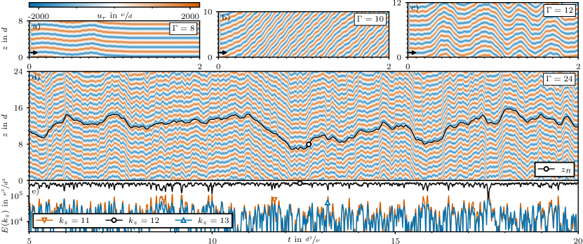
Figure 1: Spatio-temporal dynamics of Taylor rolls w.r.t. the domain size ($\Gamma$). Shown are colour-contours of the radial velocity ($u_{r}$) in the mid-gap extracted from DNS at $Re_{s}=$9475$$, $R_{\Omega}=$0.14$$. Arrows represent $1000$ convective time units. a): Stationary Taylor rolls. b–d): Axial motions on a viscous time scale. d): Temporal evolution of the phase angle of the dominant Fourier mode ($k_{z}=$12$$) of $u_{r}$ is plotted on top of the space-time data as a proxy for the position of the rolls ($z_{R}$) for a case with twelve pairs of counter-rotating rolls. e): Kinetic energy time series ($\langle E\left(k_{z}\right)\rangle_{r}$) for mode $k_{z}$. (Supplementary video.)

The largest eddies in turbulent flows are shaped by the boundary conditions (BC) of the fluid system (geometry, source of driving etc.), whereas the smallest ones are dictated by the fluid’s kinematic viscosity ($\nu$) and dissipation ($\epsilon$). Very large coherent motions in the flow field (or superstructures) carry a substantial part of the kinetic energy, which increases as the Reynolds number ($Re$) increases [1]. Understanding their role in transport and mixing processes is an active field of research, with many open questions being relevant for predicting and modelling environmental fluid flows [2]. In fluid systems with linear instabilities, such as Rayleigh–Bénard convection (RBC) and Taylor–Couette flow (TCF), turbulent superstructures are reminiscent of the cellular patterns close to the onset of instability [3, 4]. For the specific case of TCF, Taylor vortices emerge from the primary instability of the circular Couette flow [5], and then undergo a sequence of bifurcations [6, 7, 8], which gradually increase the spatio-temporal complexity as $Re$ increases. Seemingly, they persist in the form of turbulent Taylor rolls up to the highest $Re$ investigated to date [9, 10, 4, 11]. A recent review of turbulent Taylor–Couette flow is given by Grossmann et al. [12].

Turbulent Taylor rolls have been elucidated in experiments and direct numerical simulations (DNS) by performing temporal averages of the velocity field [13, 10, 14, 4, 15, 11], based upon the assumptions that the rolls remain stable and do not travel in axial direction ($z$). While in most laboratory experiments the cylinders are bounded by solid end walls, periodic BC are usually employed in most DNS. This renders $z$ homogeneous and enables the usage of short computational domains, which typically accommodate one or two pairs of Taylor rolls [e. g.  13, 16, 15, 11]. In these studies, typical observation times do not exceed a few hundred convective time units. This raises the questions of whether Taylor rolls remain stable and stationary up to arbitrarily long times. In cylindrical RBC cells, for example, the characteristic large-scale circulations (LSC) are known to undergo slow meandering in the naturally homogeneous (azimuthal) direction and also feature rare cessation events [17, 18]. More recently, Pandey et al. [3] revealed slow dynamics of the LSC also in a rectangular RBC cell based on doubly-periodic DNS for Rayleigh numbers up to $Ra=${10}^{7}$$. Similarly, Kreilos et al. [19] found slow, but large spanwise displacements of velocity streaks in turbulent boundary layer and Poiseuille flows.

In this Letter, we reveal a phase-transition giving rise to collective large-scale dynamics in axisymmetric Taylor–Couette flow. Beyond a critical domain size, the Taylor rolls undergo erratic drifts in axial direction. Compared to the cylinder rotation, the drift speeds are quiet small, but in general large excursions can occur on a viscous time scale. We show that the drift statistics are consistent with a random walk and argue that the drift is characterised through a diffusion coefficient. Finally, we demonstrate that drifts with similar dynamics and statistics occur for three-dimensional RBC and Poiseuille flows also on a viscous time scale.

We perform axisymmetric DNS of Taylor–Couette flow with periodic BC in $z$ for moderate shear Reynolds numbers ($Re_{s}\leq$3\text{\times}{10}^{4}$$), allowing for both, large computational domains ($\Gamma\leq$48$$) and long integration times ($t\leq$170$\nicefrac{{d^{2}}}{{\nu}}$). The simulations are based on integrating the incompressible Navier–Stokes equations forward in time ($t$) using our pseudo-spectral DNS code nsCouette [20]. In nsCouette, the equations are formulated in cylindrical coordinates ($r,\theta,z$) and rendered dimensionless using $d$, $\nicefrac{{\nu}}{{d}}$ and $\nicefrac{{d^{2}}}{{\nu}}$, as unit length, speed and time, respectively. Following Eckhardt et al. [21], we choose $Re_{s}=\nicefrac{{Ud}}{{\nu}}$, $R_{\Omega}=\nicefrac{{2d\Omega}}{{U}}$, $\eta=\nicefrac{{r_{i}}}{{r_{o}}}$ and $\Gamma=\nicefrac{{L_{z}}}{{d}}$ as set of non-dimensional control parameters. Here, $d=r_{o}-r_{i}$ is the gap width between the inner and outer cylinder, $L_{z}$ is their axial length, $U=u_{\theta,i}-\eta\,u_{\theta,o}$ is the difference in their velocities, and $\Omega=\nicefrac{{u_{\theta,o}}}{{r_{o}}}$ is the angular velocity of the outer cylinder. An important response parameter is the Nusselt number ($Nu_{s}$), which quantifies the transport of angular moment across the fluid layer [22, 23, 21]. In a first set of DNS (compiled in fig. 4), we fix all parameters, but $\Gamma$, to demonstrate the onset of large-scale dynamics with respect to the lateral domain size. In a second set (compiled in tab. 1), we fix $\Gamma$ and explore the effect of shear ($Re_{s}$) and rotation ($R_{\Omega}$). We keep $\eta=$0.99$$ fixed for all simulations to reduce curvature effects [23]. The initial conditions are tailored to trigger the desired amount of Taylor rolls ($N_{R}$) necessary to maintain their aspect ratio ($\Gamma_{R}=\nicefrac{{N_{R}}}{{\Gamma}}=1$). This we do to not alter the large-scale dynamics and the transport behaviour of the system, which are known to depend on $\Gamma_{R}$ [24, 11, 25, 26]. The highest friction Reynolds number ($Re_{\tau}=\nicefrac{{u_{\tau}d}}{{\nu}}$) measured in all DNS is $408$ (Tab. 1) and the spatial resolution in terms of viscous units (i. e. based on $Re_{\tau}$) is at least $$0.07$\leq\Delta r^{+}\leq$4.03$$ and $\Delta z^{+}=$4.89$$, which is state of the art in DNS of wall-bounded turbulence [15, 11, 27].

Small domains restrict the natural dynamics of the system, resulting in essentially stationary Taylor rolls. This is apparent from the space-time diagram of the radial velocity ($u_{r}$) in fig. 1a, here for $\Gamma=8$ with $N_{R}=8$ rolls. If we now enlarge the domain ($\Gamma\geq 10$, $\Gamma_{R}=1$), the Taylor rolls suddenly undergo large, erratic, collective drifts in $z$, that clearly evolve on a viscous time scale (Fig. 1b–d). In a domain with $N_{R}=24$ rolls, for example, the most energetic axial mode is $k_{z}=$12$$ throughout the simulation (Fig. 1e), confirming that the space-time representation of $u_{r}$ is indeed a robust way to identify Taylor rolls and to track their dynamics. Every few viscous time units (e. g. at $t\approx$17.5$$), the competition with neighbouring modes (here $k_{z}\in\{$11$,$13$\}$) represents rare attempts to switch to another system state with eleven or thirteen pairs of Taylor rolls. These attempts, however, remain unsuccessful in all our simulations.

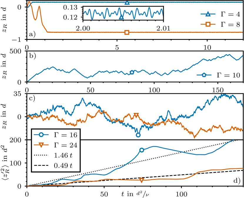
Figure 2: Taylor roll dynamics in different domains ($\Gamma$). Shown are time series of their axial drift ($z_{R}$) extracted from DNS at $Re_{s}=$9475$$, $R_{\Omega}=$0.14$$. a): Chaotic small-scale oscillations. b): Huge axial drift. c): Chaotic oscillations with large erratic drifts. d): Time series of the drift variance ($V(z_{R}$) and linear fits (Broken lines).

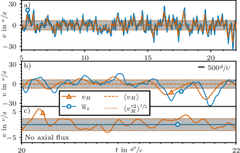
Figure 3: Taylor roll dynamics for $Re_{s}=$9475$$, $R_{\Omega}=$0.14$$, $\Gamma=$24$$. a): Time series of the drift speed ($v_{R}$) and the net axial flux ($\overline{u}_{z}$) for the case in fig. 1d. b): Zoom of panel a. The dash represents $500$ convective time units. c): Time series from DNS with $\overline{u}_{z}=0$.

To analyse the drift more quantitatively, we compute axial Fourier spectra of $u_{r}$ (space-time data as in fig. 1d) and use the phase angle of the dominant mode (here $k_{z}=12$) to approximate the location of the rolls ($z_{R}$). The temporal evolution of $z_{R}$ aligns well with $u_{r}$ (Fig. 1d), thereby confirming its suitability to quantify the drift. Figure 2 compares time series of $z_{R}$ for different domains. For $\Gamma\leq$8$$, the rolls undergo small transient drifts in the beginning of the simulation and then settle down to a fixed location, where they oscillate with tiny amplitudes and high frequencies (Fig. 2a). By contrast, for $\Gamma=$10$$ the Taylor rolls tramp more than $$100$d$ before turning back for the first time, and continue moving erratically thereafter (Fig. 2b). With further increasing $\Gamma$, the excursions become less extreme and $z_{R}$ time series for different domains look more alike (Fig. 2c). For all $\Gamma\in\{12,16,24,48\}$, the Taylor rolls undergo permanent chaotic small-scale movements with episodes of larger excursions every few $\nicefrac{{d^{2}}}{{\nu}}$. Additionally, we compute the drift speed ($v_{R}=\dot{z}_{R}$) and measure the net axial flux ($\propto\overline{u}_{z}=\nicefrac{{1}}{{\pi(r_{o}^{2}-r_{i}^{2})}}\int\!u_{z}\,r\,\text{d}r\,\text{d}\theta$), to further elucidate the large-scale dynamics. Both quantities reach values up to $$30$\nicefrac{{\nu}}{{d}}$ (Fig. 3a), corresponding to $$0.003$U$ for $Re_{s}=$9475$$.

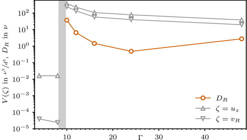
Figure 4: Phase transition for the onset of large, erratic drifts of Taylor rolls w.r.t. the domain length ($\Gamma$). Shown are variances of the drift speed ($v_{R}$) and the net axial flux ($\overline{u}_{z}$) extracted from DNS at $Re_{s}=$9475$$, $R_{\Omega}=$0.14$$. The grey area marks the critical domain. Beyond that point the axial drift is characterised by an effective diffusion coefficient ($D_{R}$).

To analyse the Taylor roll dynamics statistically, we compute the variance as $V(\zeta)=\langle\zeta^{2}\rangle-\langle\zeta\rangle^{2}$ for $\zeta\in\{z_{R},v_{R},\overline{u}_{z}\}$. Angled brackets denote temporal averaging for at least $$60$\nicefrac{{d^{2}}}{{\nu}}$ (depending on $\Gamma$), where we generally discard the first $$2$\nicefrac{{d^{2}}}{{\nu}}$ to ignore initial transients (Fig. 2a). Figure 4 compares $V(v_{R})$ and $V(\overline{u}_{z})$ for all $\Gamma$ in our first set of simulations. Both quantities reflect a sharp phase transition with a critical domain length of $$8$<\Gamma_{c}<$10$$. Beyond that critical point, variances are at least three orders of magnitudes larger compared to the sub-critical regime, clearly marking a dramatic change in the dynamics. For $\Gamma\in\{$10$,$12$\}$, variances are even higher, reflecting especially active Taylor rolls close to the critical point. Further away, however, the drift statistics seem to become invariant w.r.t. $\Gamma$, rendering the large-scale dynamics of the Taylor rolls intrinsic to the TCF system. In contrast to $V(v_{R})$ and $V(\overline{u}_{z})$, $V(z_{R})$ does not converge for $\Gamma>\Gamma_{c}$. Instead, it grows approximately linearly with time (Fig. 2c), as in a standard Wiener process. With this in mind, we estimate an effective diffusion coefficient for the drift ($D_{R}$) as the slope of a linear fit to the $V(z_{R})$ data (Fig. 2c). For sub-critical domains without erratic large-scale drift, $D_{R}=$0$$. But for $\Gamma>\Gamma_{c}$, $D_{R}$ is non-zero and seems to saturate as $\Gamma$ increases to a value that is of the order of the fluid’s kinematic viscosity (Fig. 4).

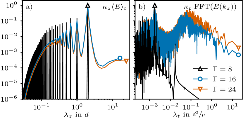
Figure 5: Transition from temporal to spatio-temporal chaos in axisymmtric Taylor–Couette flow at $Re_{s}=$9475$$, $R_{\Omega}=$0.14$$ w.r.t. the domain length ($\Gamma$). a): Time averaged, pre-multiplied axial Fourier spectra of the $u_{r}$ data (Fig. 1a–d) versus axial wavelengths $\lambda_{z}=\nicefrac{{2\pi}}{{\kappa_{z}}}$. b): Pre-multiplied temporal Fourier spectra of the modal kinetic energy (Fig. 1e) for the dominant mode (e. g. $k_{z}=$4$$ for $\Gamma=$8$$) versus temporal wavelengths $\lambda_{t}=\nicefrac{{2\pi}}{{\kappa_{t}}}$. All spectra scaled in arbitrary units.

To examine the nature of the phase transition, we now compare spatial and temporal Fourier spectra from sub- and super critical domains (Fig. 5). For $\Gamma=8$, the axial Fourier spectrum of $u_{r}$ presents discrete peaks at wavelength $\lambda_{z}=2d$ and its harmonics only (Fig. 5a). This implies that the flow state consists of four perfectly synchronised replicas of one pair of Taylor rolls. In fact, when comparing this state to those obtained for $\Gamma\in\{2,4\}$, the same Nusselt numbers ($\langle Nu_{s}\rangle=$12.824\,76$$) and spectra (not shown) are recovered. However, the temporal dynamics of the Taylor rolls is clearly chaotic, since the temporal spectra of both, the $Nu_{s}$ signal (not shown) and the kinetic energy in the dominant wavelength ($\lambda_{z}=2d$), are continuously excited (Fig. 5b). By contrast, the flow states obtained for $\Gamma\geq$10$$ additionally exhibit continuously excited spatial spectra (Fig. 5a). A similar transition from temporal to spatio-temporal chaos has been reported before for mechanically [28] and magnetically [29] forced TCF. Note, that the transition is also reflected in the mean Nusselt number, but only in the third digit ($\langle Nu_{s}\rangle=$12.78$\pm$0.04$$ for all $\Gamma$). What is remarkable here is that the onset of spatio-temporal chaos coincides with the onset of large-scale drifts of the roll pattern. For $\Gamma>\Gamma_{c}$ the temporal spectra exhibit two dominant time scales, which clearly separate the fast (turbulent) fluctuations from the much slower drift dynamics of the Taylor rolls (Fig. 5b). The latter is associated to nonlinear interactions of the wavelength $\lambda_{z}\approx$2$d$ with other modes, which together excite the fundamental wavelength $\lambda_{z}=L_{z}$. We note that, whilst much effort has been dedicated to remove drifts in the analysis of turbulent dynamics in wall-bounded flows [e. g.  30, 31], here the onset of spatio-temporal chaos appears intrinsically linked to the slow, erratic drift dynamics.

Table 1: Taylor roll dynamics for different set-ups and $\Gamma=24$. Listed are control parameters ($Ra$, $Re_{s}$, $R_{\Omega}$, no axial flux), response parameters ($Nu_{s}$, $Nu$, $Re_{\tau}$) and standard deviations of the drift speed ($v_{R}$) and net axial flux ($\overline{u}_{z}$).

$Ra$	$Re_{s}$	$R_{\Omega}$	NoFX		$Nu_{s}$	$Nu$	$Re_{\tau}$		$\sqrt{\langle v_{R}^{\prime 2}\rangle}$	$\sqrt{\langle\overline{u}_{z}^{\prime 2}\rangle}$
${10}^{5}$	$925$	$0.14$			$4.6$		$33$		${10}^{-15}$	${10}^{-14}$
${10}^{6}$	$2940$	$0.14$			$7.4$		$74$		$0.4$	$1.1$
${10}^{7}$	$7138$	$0.30$			$10.4$	$14.4$	$137$		$6.2$	$8.0$
${10}^{7}$	$9475$	$0.14$			$12.8$	$14.7$	$175$		$6.3$	$8.6$
${10}^{7}$	$9475$	$0.14$	$\times$		$12.8$		$175$		$2.3$	${10}^{-6}$
${10}^{7}$	$15\,779$	$0.05$			$14.6$	$15.3$	$241$		$7.4$	$9.6$
${10}^{8}$	$29\,539$	$0.14$			$22.4$		$408$		$12.0$	$13.8$

Now we exploit an analogy between rotating and stratified flows [32, 33, 8, 22, 21], to demonstrate that both systems, RBC and TCF, exhibit this remarkable drift dynamics. According to the exact Navier–Stokes mapping of Eckhardt et al. [21], two axisymmetric TCF systems with vanishing curvature ($\eta\rightarrow$1$$) are exactly identical as long as $Ra=Re_{s}^{2}R_{\Omega}\left(1-R_{\Omega}\right)=\text{const}$. As a consequence, their drift dynamics must be identical too. Indeed, for moderate rotation ($R_{\Omega}\in\{$0.14$,$0.30$\}$), the drift statistics are very similar (Tab. 1) and the same is true for the corrected Nusselt number ($Nu=1+\nicefrac{{Nu_{s}-1}}{{1-R_{\Omega}}}$) [21]. We attribute the small deviations to the presence of small yet finite curvature effects ($\eta=0.99<1$), which are not included in the analogy. However, for very slow rotation ($R_{\Omega}=$0.05$$), the drift statistics deviate noticeably. The exact analogy breaks down in the limit of a stationary outer cylinder ($R_{\Omega}=0$), but we expect that discrepancies due to non-vanishing curvature effects grow progressively as this limit is approached.

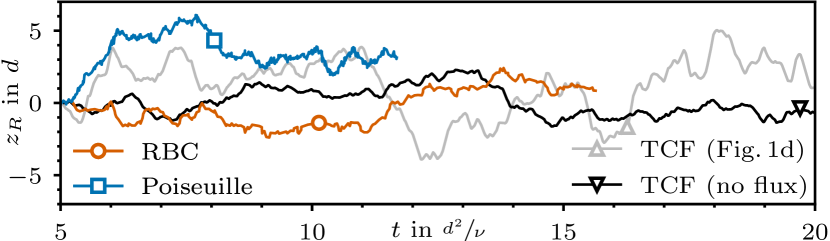
Figure 6: Large-scale drift ($z_{R}$) in different fluid systems: Axial Taylor roll drift in axisymmetric TCF with and without net axial flux. Azimuthal meandering of convection rolls in an eleven days lab experiment in a cylindrical RBC cell [17]. Spanwise streak displacement in Poiseuille flow [19]. Results from another $33$ days RBC experiment [18] look similar and are thus not shown.

To investigate how the axial drift depends on the level of turbulence, we repeat our analysis for different $Ra$ by varying $Re_{s}$ and fixing $R_{\Omega}$. Table 1 shows that the Taylor rolls become more active with increasing $Re_{s}$. This is consistent with experiments Xi et al. [18], showing that the rms increment of the rotation angle of the LSC increases tenfold as $Ra$ increases from ${10}^{9}$ to ${10}^{10}$. Figure 6 compares the underlying time signal of this rotation [17, 18] to drift signals extracted from our DNS and a time signal of large spanwise streak displacements in Poiseuille flow [19]. For the sake of comparison, the rotation angle is converted to a length using the radius of the RBC cell and all drift signals are shown in the viscous time scale, which is also the relevant one of the aforementioned analogy [21]. The general qualitative agreement is remarkable, indicating that these viscous-time scale dynamics might be inherent to many different fluid systems. Note, that the longest time series considered here (Fig. 2) correspond to $$170$Re_{s}=\mathcal{O}\!\left(${10}^{6}$\right)$ convective time units and to $$170$\sqrt{Ra}=\mathcal{O}\!\left(${10}^{5}$\right)$ free-fall time units in case of Rayleigh–Bénard convection ($Ra=${10}^{7}$$). These observation times are comparable to those used to characterise large-scale states in RBC [3, 25], but they are several orders of magnitudes longer compared to typically integration times in high-$Re$ TCF studies [16, 4, 15, 11]. In the TCF apparatus of Huisman et al. [4], for example, this would corresponds to a measurement time of twelve days. For flows in nature, this implies that the time scale necessary to observe such changes in the large-scale dynamics may be enormous. This is consistent, for example, with changes observed in the large-scale structure of Earth’s magnetic field (magnetic reversals), which coincidentally also occur on a diffusive time scale [34].

Furthermore, we find that $\overline{u}_{z}$ is strongly correlated to $v_{R}$ (Fig. 3a). This raises the question of whether the drift of the Taylor rolls causes the net axial flux, or vice-versa, or if both phenomena have a common driver that is neither of them. Figure 3b shows that $v_{R}$ is approximately $$500$\nicefrac{{d}}{{U}}$ ahead of $\overline{u}_{z}$, suggesting the former. We probe this hypothesis by suppressing the axial flux in our DNS, as is the case in systems with axial end walls [35]. As a result, $v_{R}$ is substantially reduced (Fig. 3c) and its variance decreases by a factor of three (Tab. 1), but otherwise the drift dynamics remains unaltered (Fig.6). We stress that neither the onset of drifts nor suppressing the axial flux, does alter the integral transport, as the Nusselt number remains unchanged within three digits in all cases.

Future work should address whether this phenomenon persists in three-dimensional TCF simulations and can be observed experimentally. Moreover, the newly found drift of Taylor rolls should be compared in more detail to the slow azimuthal LSC drifts in cylindrical RBC [17, 18] and the simplified models developed to describe them. More specifically, do the drift velocities follow a Gaussian, Poissonian or bi-modal distribution in time? It would also be interesting to test if and how the critical domain size for the onset of large-scale dynamics changes with Reynolds (Rayleigh) number.

We appreciate stimulating discussions with Alberto Vela-Martín and we gratefully acknowledge financial support from the German Research Foundation (DFG) through the priority programme Turbulent Superstructures (SPP1881) and computational resources provided by the North German Supercomputing Alliance (HLRN) through project hbi00041.

References

- Smits et al. [2011] A. J. Smits, B. J. McKeon, and I. Marusic, High-Reynolds number wall turbulence, Annual Review of Fluid Mechanics 43, 353 (2011).
- Dauxois et al. [2021] T. Dauxois, T. Peacock, P. Bauer, C. P. Caulfield, C. Cenedese, C. Gorlé, G. Haller, G. N. Ivey, P. F. Linden, E. Meiburg, N. Pinardi, N. M. Vriend, and A. W. Woods, Confronting Grand Challenges in environmental fluid mechanics, Physical Review Fluids 6, 020501 (2021).
- Pandey et al. [2018] A. Pandey, J. D. Scheel, and J. Schumacher, Turbulent superstructures in Rayleigh-Bénard convection, Nature Communications 9, 1 (2018).
- Huisman et al. [2014] S. G. Huisman, R. C. Van Der Veen, C. Sun, and D. Lohse, Multiple states in highly turbulent Taylor-Couette flow, Nature Communications 5, 1 (2014).
- Taylor [1923] G. I. Taylor, Stability of a viscous liquid contained between two rotating cylinders, Philosophical Transactions of the Royal Society of London. Series A, Containing Papers of a Mathematical or Physical Character 223, 289 (1923).
- Coles [1965] D. Coles, Transition in circular Couette flow, Journal of Fluid Mechanics 21, 385 (1965).
- Fenstermacher et al. [1979] P. R. Fenstermacher, H. L. Swinney, and J. P. Gollub, Dynamical instabilities and the transition to chaotic Taylor vortex flow, Journal of Fluid Mechanics 94, 103 (1979).
- Prigent et al. [2006] A. Prigent, B. Dubrulle, O. Dauchot, and I. Mutabazi, The Taylor-Couette Flow: The Hydrodynamic Twin of Rayleigh-Bénard Convection, in Dynamics of Spatio-Temporal Cellular Structures, Springer Tracts in Modern Physics, Vol. 207, edited by I. Mutabazi, J. E. Wesfreid, and E. Guyon (Springer New York, 2006) pp. 225–242.
- Lathrop et al. [1992] D. P. Lathrop, J. Fineberg, and H. L. Swinney, Transition to shear-driven turbulence in Couette-Taylor flow, Physical Review A 46, 6390 (1992).
- Ravelet et al. [2010] F. Ravelet, R. Delfos, and J. Westerweel, Influence of global rotation and Reynolds number on the large-scale features of a turbulent Taylor-Couette flow, Physics of Fluids 22, 1 (2010).
- Ostilla-Mónico et al. [2016a] R. Ostilla-Mónico, D. Lohse, and R. Verzicco, Effect of roll number on the statistics of turbulent Taylor-Couette flow, Physical Review Fluids 1, 054402 (2016a).
- Grossmann et al. [2016] S. Grossmann, D. Lohse, and C. Sun, High-Reynolds Number Taylor-Couette Turbulence, Annual Review of Fluid Mechanics 48, 53 (2016).
- Dong [2007] S. Dong, Direct numerical simulation of turbulent Taylor–Couette flow, Journal of Fluid Mechanics 587, 373 (2007).
- Ostilla-Mónico et al. [2013] R. Ostilla-Mónico, R. J. Stevens, S. Grossmann, R. Verzicco, and D. Lohse, Optimal Taylor-Couette flow: Direct numerical simulations, Journal of Fluid Mechanics 719, 14 (2013).
- Ostilla-Mónico et al. [2016b] R. Ostilla-Mónico, R. Verzicco, S. Grossmann, and D. Lohse, The near-wall region of highly turbulent Taylor-Couette flow, Journal of Fluid Mechanics 788, 95 (2016b).
- Brauckmann and Eckhardt [2013] H. J. Brauckmann and B. Eckhardt, Direct numerical simulations of local and global torque in Taylor-Couette flow up to Re = 30 000, Journal of Fluid Mechanics 718, 398 (2013).
- Brown and Ahlers [2006] E. Brown and G. Ahlers, Journal of Fluid Mechanics, Vol. 568 (2006) pp. 351–386.
- Xi et al. [2006] H.-D. Xi, Q. Zhou, and K.-Q. Xia, Azimuthal motion of the mean wind in turbulent thermal convection, Physical Review E 73, 056312 (2006).
- Kreilos et al. [2014] T. Kreilos, S. Zammert, and B. Eckhardt, Comoving frames and symmetry-related motions in parallel shear flows, Journal of Fluid Mechanics 751, 685 (2014).
- López et al. [2020] J. M. López, D. Feldmann, M. Rampp, A. Vela-Martín, L. Shi, and M. Avila, nsCouette – A high-performance code for direct numerical simulations of turbulent Taylor–Couette flow, SoftwareX 11, 100395 (2020).
- Eckhardt et al. [2020] B. Eckhardt, C. R. Doering, and J. P. Whitehead, Exact relations between Rayleigh–Bénard and rotating plane Couette flow in two dimensions, Journal of Fluid Mechanics 903, R4 (2020).
- Eckhardt et al. [2007] B. Eckhardt, S. Grossmann, and D. Lohse, Fluxes and energy dissipation in thermal convection and shear flows, Europhysics Letters (EPL) 78, 24001 (2007).
- Brauckmann et al. [2016] H. J. Brauckmann, M. Salewski, and B. Eckhardt, Momentum transport in Taylor–Couette flow with vanishing curvature, Journal of Fluid Mechanics 790, 419 (2016).
- Ostilla-Mónico et al. [2015] R. Ostilla-Mónico, R. Verzicco, and D. Lohse, Effects of the computational domain size on direct numerical simulations of Taylor-Couette turbulence with stationary outer cylinder, Physics of Fluids 27, 025110 (2015).
- Wang et al. [2020] Q. Wang, R. Verzicco, D. Lohse, and O. Shishkina, Multiple States in Turbulent Large-Aspect-Ratio Thermal Convection: What Determines the Number of Convection Rolls?, Physical Review Letters 125, 074501 (2020).
- Zwirner et al. [2020] L. Zwirner, A. Tilgner, and O. Shishkina, Elliptical Instability and Multiple-Roll Flow Modes of the Large-Scale Circulation in Confined Turbulent Rayleigh-Bénard Convection, Physical Review Letters 125, 054502 (2020).
- Feldmann et al. [2021] D. Feldmann, D. Morón, and M. Avila, Spatiotemporal intermittency in pulsatile pipe flow, Entropy 23, 1 (2021).
- Avila et al. [2007] M. Avila, F. Marques, J. M. Lopez, and A. Meseguer, Stability control and catastrophic transition in a forced Taylor–Couette system, Journal of Fluid Mechanics 590, 471 (2007).
- Guseva et al. [2015] A. Guseva, A. P. Willis, R. Hollerbach, and M. Avila, Transition to magnetorotational turbulence in Taylor-Couette flow with imposed azimuthal magnetic field, New Journal of Physics 17, 10.1088/1367-2630/17/9/093018 (2015).
- Willis et al. [2013] A. P. Willis, P. Cvitanović, and M. Avila, Revealing the state space of turbulent pipe flow by symmetry reduction, Journal of Fluid Mechanics 721, 514 (2013).
- Budanur et al. [2015] N. B. Budanur, P. Cvitanović, R. L. Davidchack, and E. Siminos, Reduction of SO(2) symmetry for spatially extended dynamical systems, Physical Review Letters 114, 1 (2015).
- Bradshaw [1969] P. Bradshaw, The analogy between streamline curvature and buoyancy in turbulent shear flow, Journal of Fluid Mechanics 36, 177 (1969).
- Veronis [1970] G. Veronis, The Analogy Between Rotating and Stratified Fluids, Annual Review of Fluid Mechanics 2, 37 (1970).
- Hollerbach and Jones [1993] R. Hollerbach and C. A. Jones, Influence of the Earth’s inner core on geomagnetic fluctuations and reversals, Nature 365, 541 (1993).
- Marques and Lopez [1997] F. Marques and J. M. Lopez, Taylor–Couette flow with axial oscillations of the inner cylinder: Floquet analysis of the basic flow, Journal of Fluid Mechanics 348, 153 (1997).