The spin-one Motzkin chain is gapped for any area weight $t<1$

Abstract

We prove a conjecture by Zhang, Ahmadain, and Klich that the spin-$1$ Motzkin chain is gapped for any area weight $t<1$. Existence of a finite spectral gap is necessary for the Motzkin Hamiltonian to belong to the Haldane phase, which has been argued to potentially be the case in recent work of Barbiero, Dell’Anna, Trombettoni, and Korepin. Our proof rests on the combinatorial structure of the ground space and the analytical verification of a finite-size criterion.

1 Introduction and main results

Since quantum matter often resides in its ground space, the investigation of ground state properties and of the energy gap to the first excited state are central topics of study in quantum many-body theory. The existence of a spectral gap implies an area law for the entanglement entropy in one-dimensional (1D) physical spin systems and certain two-dimensional (2D) models [Has07, AAG21]. The converse is false; an area law does not necessarily imply a gap, as can be seen from integrable toy models such as the XY spin chain in a random field. Furthermore, vanishing of the spectral gap is a necessary condition for the existence of a quantum phase transition.

In this paper, we investigate the spectral gap of a special class of 1D quantum spin systems whose ground states can be characterized analytically. The original Motzkin spin chain is a 1D local spin-$1$ Hamiltonian that was introduced in [BCM⁺12] as a toy model. This model has a unique frustration-free ground state which has an exact representation as a uniform superposition of Motzkin walks from classical probability theory. This work was then generalized by Movassagh and Shor to any integer spin $s\geq 1$ in [MS16] and called $s-$colored Motzkin quantum spin chain, where each color represents a spin value $s$. In particular, it was proved that for any number of colors $s>1$ the model exhibits tremendous amount of entanglement in its ground state which was not previously believed possible for ground states of physical quantum spin chains. Later, Korepin et al. found that the $s-$colored Motzkin chain is an unusual integrable model [TSHK21]. The frustration-freeness along with the combinatorial nature of the ground state structure allows one to map these quantum models to classical Markov processes in classical probability theory for analyzing the entanglement entropy of the ground state and the gap above the ground state. To make this precise, we recall that, given a chain of length $2L$, the entanglement entropy between the left and right halves is given by $S(\rho_{L})=-\mathrm{tr}\rho_{L}\log\rho_{L}$ with $\rho_{L}$ the reduced density matrix of the ground states on the left half of the chain. In [MS16] it was proved that ground states of Motzkin chains with at least two colors have a half-chain entanglement entropy of $S(\rho_{L})\sim\sqrt{L}$. (This is a consequence of the universality of Brownian motion in which the random Motzkin walks typically reach the height of $O(\sqrt{L})$ in the middle of the chain.) Since there are $s^{O(\sqrt{L})}$ ways of coloring each walk, the entanglement entropy between the two halves is expected to be $\sqrt{L}\log{s}$. This is noteworthy because one only finds $S(\rho_{L})\sim\log L$ for translation-invariant critical systems in 1D. The latter was the basis of the belief that physical local Hamiltonians in 1D cannot sustain super-critical (i.e., super logarithmic in the system’s size) amount of entanglement.

A key innovation appeared in the 2016 work of Zhang, Ahmadein, and Klich [ZAK17] who introduced a tilting parameter $t>0$ into the local interaction such that the ground state becomes a grand-canonical superposition of Motzkin walks in which each walks is weighted by $t^{\mathrm{area}}$. They proved that area-weighted Motzkin chains undergo a novel entanglement phase transition at area weight $t=1$: For $t<1$, the entanglement entropy $S(\rho_{L})\lesssim 1$ is a constant and for $t>1$, and at least two colors (i.e., $s\geq 2$), $S(\rho_{L})\sim L$ is extensive (which is the maximal $L$-scaling for entanglement entropy). Motzkin spin chains have since blossomed into novel paradigm Hamiltonians that allow to flexibly dial entanglement with a single parameter. For example, Motzkin spin chains have been used in quantum error-correcting codes [BCŞB19], with their generalizations being “good quantum codes”[MO20]. Moreover, they generate exact holographic tensor network representations [AEK21] and have connections to number theory [HSK22].

In the same 2016 paper, Zhang, Ahmadein, and Klich (ZAK) conjectured that the area-weighted Motzkin spin chains are gapped for area weight $t<1$ and any color. This conjecture remained open until now. Upper bounds on the closing rate of the spectral gap exist for $t=1$ and $s\geq 1$ [BCM⁺12, MS16] and for $t>1$ and $s\geq 2$ [LM17].

One motivation for the ZAK conjecture is Hastings’ result [Has07] that a gap would imply the area law $S(\rho_{L})\lesssim 1$ found by ZAK. A subsequent numerical study of the $t<1$ system [BDTK17] found further evidence for a spectral gap as well as hallmarks of Haldane topological order. These findings have put additional emphasis on the [ZAK17] conjecture because the spectral gap is central to the classification scheme of topological order.

Our main result rigorously proves that the spin-$1$ Motzkin chain is gapped for any area weight $t<1$ as conjectured by Zhang, Ahmadein, and Klich.

We recall that “gapped” means that there exists a constant gap independent of the system size. Our result establishes that the spin-$1$ and $t<1$ Motzkin spin chains belong to a different quantum phase than the highly entangled $t\geq 1$ Motzkin Hamiltonians with at least two colors. The $t<1$ phase is expected to be closely related to the quantum phase of the AKLT chain [AKLT88], also called Haldane phase, with the all-important gap being established by the present work.

Let us now state the main result precisely. Given area weight $t>0$, let $H_{n}(s,t)$ be the Motzkin Hamiltonian on a chain of length $n$ as introduced in [ZAK17] and recalled in Subsection 2.1 below. We write $\gamma_{n}(t)$ for its spectral gap.

Theorem 1.1 (Main result—spectral gap).

For every $t\in(0,1)$, there exists a constant $c(t)>0$ such that

$$\gamma_{n}(t)\geq c(t)>0,\qquad\textnormal{for all }n\geq 1.$$ (1.1)

The important point is that the constant $c(t)>0$ does not depend on the system size and thus the lower bound extends to the thermodynamic limit.

1.1 Ideas in the proof

Let us briefly discuss the main proof ideas. The overarching idea is to use a finite-size criterion for the existence of a spectral gap. In recent years, various finite-size criteria have been successfully applied to frustration-free Hamiltonians including higher-dimensional ones [ARLL⁺20, GPW21, JL21, Lem19, LN19, LSY19, LSW20, MM21, Nac96, PW19, PW20, WY21, WY21]. Here we use an idea of Fannes-Nachtergaele-Werner [FNW92] based on estimating the angle between local ground spaces which is reminiscient of, but different from the martingale method and has played a central role in the recent works [ARLL⁺20, GPW21, PW19, PW20]; see also [SS03]. Our finite-size criterion is based on the same general idea and reduces the spectral gap problem to bounding the ground state overlap $\|G_{[k+1,3k]}G_{[1,2k]}-G_{[1,3k]}\|<{1\over 2}$ which roughly speaking measures the “delocalization” of possible excitations. See Theorem 4.3 for the precise statement of the finite-size criterion. The norm $\|G_{[k+1,3k]}G_{[1,2k]}-G_{[1,3k]}\|$ can be calculated solely in terms of states $|{\phi}\rangle$ on the full chain which are excited (orthogonal to the full-chain ground space), but their components on the first two-thirds of the chain are local ground states. We then ask how much these states can overlap with the ground space on the last two-thirds of the chain, and show that the answer is almost not at all, thus verifying our finite-size criterion.

The proof of Theorem 1.1 requires several new ideas. In particular, the following two technical challenges arise when we decompose the Motzkin Hamiltonian into subsystems to verify the finite-size criterion and need to be addressed:

• The Motzkin walks are pinned to have an initial up or flat step and final down or flat step through particular boundary projectors. This leads to a particular breaking of translation-invariance and different kinds of subsystem Hamiltonians at the bulk versus boundaries.

• The ground space of each subsystem relevant to the finite-size criterion (which naturally comes with open boundary conditions) is highly degenerate; the dimension scales like system size squared. When composing Motzkin subchains, this degeneracy leads to massive combinatorial factors which have to be a posteriori balanced by the area weight.

To address the first point, we develop a scheme to remove the boundary projectors and reduce the derivation of the gap to the gap of the Motzkin Hamiltonian with open boundary conditions. For this, we rely on Kitaev’s projection lemma [KKR06] and an explicit calculation of the boundary energy penalty incurred by superpositions Motzkin walks not satisfying the boundary conditions. See Subsections 2.3 and 2.4 for the details.

To address the more difficult second point, we introduce a notion of approximate ground states to ameliorate some of the massive combinatorial issues. Our approximation scheme is based on the observation that a ground state of the open chain with $p$ unbalanced up steps and $q$ unbalanced down steps will tend to have the up-steps accumulating on the left end and the down-steps accumulating on the right end of the chain because of the exponential weighting of area. This notion of approximate ground state and the analysis of their overlap, which is central to the verification of the finite-size criterion, are at the heart of our paper and will be explained further in due course. Moreover, working with approximate ground states, which are themselves superpositions of unbalanced Motzkin walks, requires carefully tracking of the $p$- and $q$-dependence of their normalization factors. This can be done by an elementary, but surprisingly technical induction scheme based on heuristically viewing the recursion relation of normalization factors as a spatially inhomogeneous 1D discrete diffusion equation; see Appendix A. It will be interesting to see if the rather precise descriptions of raised ground states and their normalizations that we find in this work have applications beyond the spectral gap problem, e.g., for the combinatorial problems involved with studying entanglement entropy and correlation functions at multiple scales, or perhaps to shed light on the potential topological order of the ground state.

Regarding alternative techniques, we first mention that the martingale method with finite overlap does not seem to apply in our model for values of $t$ arbitrarily close to $1$, basically, because the relevant systems entering it have small overlap compared to their size. See the Remark Remark. This is different in our finite-size criterion where the relevant subsystems overlap approximately to 50%.

We also recall that alternative finite-size criteria exist that are based on Knabe’s original idea [Kna88]; see [Ans20, GM16, Lem20, LM19, LX21]. These can be used to derive the spectral gap for sufficiently small $t$, specifically, we have successfully verified a similar finite-size criterion [LM19] numerically for $t\leq 0.55$. However, it is clear that a fully analytical argument is required to cover the full range of $t\in(0,1)$ . This is what we supply in this paper.

For readers familiar with the literature on Motzkin spin chains, we mention that we do not reformulate the gap problem as a gap problem for classical Markov chains as was done in [LM17, Mov18, MS16]. This has two reasons: (i) Even with the reformulation, one would still have to derive a new non-trivial classical probability result, namely existence of an order-$1$ gap for the appropriate classical Markov chain. (ii) As the above works show, this approach commonly incurs losses of factors depending on the systems size. This makes it well suitable for proving that the gap closes polynomially for $t=1$ regime or exponentially in the $t>1$ regime. However, the present case is more delicate because we aim to derive an order-$1$ lower bound on the gap and such system-size dependent losses, even just logarithm ones, can no longer be afforded. Nonetheless, it would be interesting to see an alternative derivation of our main result via purely probabilistic techniques. Conversely, our result can be used to derive the spectral gap of the corresponding classical Markov chain, which may be of independent interest.

We close the introduction by mentioning some open problems. First, it is natural to aim to extend the result to higher spin while keeping $t\in(0,1)$ arbitrary. Second, the Motzkin spin chains are “bosonic” in the sense that the local spin number is an integer. Their “fermionic” siblings with half-integer spin are called Fredkin spin chains and have also been studied in detail [Mov18, UK17, ZK17]. While the local interaction on the Fredkin side is slightly more subtle (it is $3$-local instead of nearest-neighbor as in the Motzkin case), the developments there are essentially parallel and we generally expect these models to be amenable to our technique.

1.2 Organization of the paper

In Section 2, we introduce the main model, the Motzkin Hamiltonian with pinning boundary conditions. We also introduce it with open boundary conditions and explain how a spectral gap with open boundary conditions implies the main result via Kitaev’s projection lemma [KKR06].

In Section 3, we give a precise characterization of open-chain ground states by extending the analysis of [ZAK17] and use this characterization to infer the important boundary energy penalty of raised ground states mentioned above.

In Section 4, we formulate our finite-size criterion for general frustration-free open spin chains (Theorem 4.3) based on the duality projection lemma of [FNW92].

Sections 5-10 and two appendices contain the technically challenging analytical verification of the finite-size criterion for any $t<1$. The proof strategy for these parts is summarized later, in Section 5.

2 The model and the proof of the main result

2.1 The Motzkin Hamiltonian

The Motzkin Hamiltonian is defined on a chain of $n$ spin-$1$ particles, so the total Hilbert space is $\bigotimes_{j=1}^{n}\mathbb{C}^{3}$. We label the basis states as up-, down- or null-steps, i.e., $\mathbb{C}^{3}=\mathrm{span}\{|{u}\rangle,|{d}\rangle,|{0}\rangle\}$. Following ZAK [ZAK17], we define for any area weight $t>0$, the Motzkin Hamiltonian

$$H_{n}(t)=\Pi_{bdry}+\sum_{j=1}^{n-1}\Pi_{j,j+1}(t)$$ (2.1)

with local interactions

$$\Pi_{\text{bdry}} =|{d}\rangle\langle{d}|_{1}+|{u}\rangle\langle{u}|_{n}$$ (2.2)

$$\Pi_{j,j+1}(t) =|{U(t)}\rangle\langle{U(t)}|_{j,j+1}+|{D(t)}\rangle\langle{D(t)}|_{j,j+1}+|{\varphi(t)}\rangle\langle{\varphi(t)}|_{j,j+1}$$ (2.3)

where

$$|U(t)\rangle =\frac{1}{\sqrt{1+t^{2}}}\Big{(}t\cdot|{0u}\rangle-|{u0}\rangle\Big{)}$$ (2.4)

$$|D(t)\rangle =\frac{1}{\sqrt{1+t^{2}}}\Big{(}|{0d}\rangle-t\cdot|{d0}\rangle\Big{)}$$ (2.5)

$$|\varphi(t)\rangle =\frac{1}{\sqrt{1+t^{2}}}\Big{(}|{ud}\rangle-t\cdot|{00}\rangle\Big{)}$$ (2.6)

We recall that $H_{n}(t)$ has a unique frustration-free ground state which is an area-weighted superposition of Motzkin walks.

Theorem 2.1 ([ZAK17]).

For every $t>0$, the zero eigenspace of $H_{n}(t)$ is spanned by the normalized ground state vector

$$|{GS_{0,0}}\rangle=\frac{1}{N_{0,0}}\sum_{w\in G_{0,0}}t^{\mathcal{A}(w)}|{w}\rangle.$$

Here $G_{0,0}$ denotes the set of Motzkin walks of length $n$ and $\mathcal{A}$ denotes the total area under the walk. Recall that a Motzkin walks is a discrete one-dimensional walk comprised of up-, down-, and flat steps, which only takes positive values, i.e., it stays above the horizontal axis.

Theorem 2.1 implies that $H_{n}(t)$ is frustration-free with zero energy ground state and so its spectral gap is equal to its smallest positive eigenvalue,

$$\gamma_{n}(t)=\inf(\mathrm{spec}\,H(t)\setminus\{0\}).$$

2.2 The Motzkin Hamiltonian with open boundary conditions

The following open-boundary Motzkin Hamiltonian will play a central role in our proof. We define

$$H^{0}_{n}(t)=\sum_{j=1}^{n-1}\Pi_{j,j+1}(t)$$ (2.7)

so that $H_{n}(t)=H_{n}^{0}(t)+\Pi_{\text{bdry}}$. We write $\gamma^{0}_{n}(t)$ for the spectral gap of $H^{0}_{n}(t)$.

As Theorem 2.4 below shows, $H^{0}_{n}(t)$ has frustration-free ground states that can be explicitly described in a similar way as in Theorem 2.1. The main difference is that, without the boundary projectors, the initial and final height of the Motzkin walk are free, leading to a degeneracy of the ground space of $H^{0}_{n}(t)$ that is quadratic in system size.

To characterize the ground states of $H_{n}^{0}(t)$ exactly, we introduce the following notions. First, notice that there is a one-to-one correspondence between basis states in the Hilbert space $\bigotimes_{j=1}^{n}\mathbb{C}^{3}$ and strings $\mathfrak{s}\in\{0,u,d\}^{n}$. General states thus correspond to linear combinations of such strings. On these, we define the local moves

$$(0u)\leftrightarrow t\text{ }(u0)\qquad t\text{ }(0d)\leftrightarrow(d0)\qquad(00)\leftrightarrow t\text{ }(ud).$$ (2.8)

Notice that by making the unit of area equal to $1$, each local move changes the area by $1$.

The key idea is to introduce an equivalence relation among (scalar multiples of) strings.

Definition 2.2 (Equivalence relation).

Two strings are equivalent if and only if they are related by a sequence of local moves:

$$\mathfrak{s_{1}}\sim\mathfrak{s_{2}}\quad\stackrel{{\scriptstyle\mathrm{def}}}{{\Longleftrightarrow}}\quad t^{{\mathcal{A}}(\mathfrak{s_{1})}}\mathfrak{s_{1}}\leftrightarrow t^{{\mathcal{A}}(\mathfrak{s_{2}})}\mathfrak{s_{2}},$$ (2.9)

where ${\mathcal{A}}(\mathfrak{s})$ is the area under the walk encoded by $\mathfrak{s}$.

Since the string $\mathfrak{s}$ only defines the corresponding walk up to an overall up- or down-shift, we use the convention that the walk corresponding to $\mathfrak{s}$ is the unique non-negative walk of minimal area. See Figure 1 for an example and Subsection 6.1 for further discussion.

The ground states will be defined in terms of the following equivalence classes of the imbalanced walks.

Definition 2.3.

For any integers $p,q\geq 0$ with $p+q\leq n$, we define the walk

$$g_{p,q}=(\underbrace{d,\dots,d}_{p},0,\dots,0,\underbrace{u,\dots,u}_{q}),$$

where the starting height is $p$, the ending height is $q$, and in between the imbalanced steps we have a string of all flat steps (zeros) at zero height; (see Fig. 1). We write $G_{p,q}$ for its equivalence class under the equivalence relation $\sim$ from (2.9).

Figure 1: Representative walk $g_{p,q}$ in the equivalence class $G_{p,q}$. Through the local moves (2.8), any walk in the $G_{p,q}$ class can be brought (with an appropriate area-dependent prefactor) to the form shown here.

Theorem 2.4 (Characterization of open-chain ground space).

The ground space of $H_{n}^{0}(t)$ is spanned by the collection of orthonormal vectors

$$|GS_{p,q}\rangle=\frac{1}{\sqrt{{N}_{p,q}}}\sum_{w\in G_{p,q}}t^{{\mathcal{A}}(w)}|w\rangle,\qquad p,q\geq 0,\quad p+q\leq n.$$ (2.10)

where ${N}_{p,q}$ is a normalization factor.

This theorem will be proved in Subsection 3.1 by generalizing ideas in [ZAK17].

The key result and main technical work of this paper is to prove that the Motzkin Hamiltonian with open boundary conditions is gapped.

Theorem 2.5 (Gap with open boundary conditions).

For every $t\in(0,1)$, there exists a constant $c_{1}(t)$ such that

$$\gamma^{0}_{n}(t)\geq c_{1}(t)>0,\qquad n\geq 2.$$ (2.11)

This result will be proved by verifying a suitable finite-size criterion presented in Section 4.

2.3 Boundary penalty of raised ground states

The fact that the Motzkin Hamiltonian $H(t)$ is equipped with special “pinning” boundary projectors makes the model highly non-translation-invariant at the boundary and not well suited for finite-size criteria. Indeed, notice that a finite-size criterion naturally concerns open boundary conditions, since it requires good understanding of subchains. (To our knowledge, the only exception to this general rule is the recent work [WY21].)

Therefore, we require a post-processing step to reduce the spectral gap problem for $H_{n}(t)$ to that of $H_{n}^{0}(t)$, i.e., to conclude Theorem 1.1 from Theorem 2.5. The basic idea for this step is as follows: Given that $H_{n}^{0}(t)$ is gapped, it is relatively clear that the gap of $H_{n}(t)$ is mainly challenged by the possibility that members of the ground state family $|{GS_{p,q}}\rangle$ (described in Theorem 2.4 above) could have small excitation energy with respect to the boundary projector, thereby closing the gap. We are able to exclude this possibility by Proposition 2.7 below.

Definition 2.6.

Let $G^{n}\subset\big{(}\mathbb{C}^{3}\big{)}^{\otimes n}$ be the collection of raised ground states of $H_{n}^{0}(t)$,

$$G^{n}=\text{span}\{|{GS_{p,q}}\rangle:p,q\geq 0,\,1\leq p+q\}.$$ (2.12)

Proposition 2.7 (Boundary penalty of raised ground states).

For every $t\in(0,1)$, there exists a constant $c_{2}(t)$ such that

$$\lambda_{min}\left(\Pi_{\text{bdry}}|_{G^{n}}\right)\geq c_{2}(t)>0,\qquad n\geq 1$$ (2.13)

2.4 Proof of the main result

Thanks to Proposition 2.7 we can now derive the spectral gap of the Moztkin Hamiltonian with pinning boundary conditions from Theorem 2.5 via an application of Kitaev’s projection lemma [KKR06].

Proof of Theorem 1.1 assuming Theorem 2.4.

Throughout the proof, we always restrict to the subspace $|{GS_{0,0}}\rangle^{\perp}\subset(\mathbb{C}^{3})^{\otimes n}$, the orthogonal complement of the ground state $|{GS_{0,0}}\rangle$. We suppress this restriction from the notation, i.e., we identify $H_{n}\equiv H_{n}|_{|{GS_{0,0}}\rangle^{\perp}}$, etc. The claim that $H_{n}$ has a uniform spectral gap when considered on the whole space now translates to the bound

$$\lambda_{min}\left(H_{n}\right)\geq c(t)>0$$ (2.14)

where $c(t)>0$ should be independent of the system size $n$. Let $0<\epsilon\leq 1$. We define the operator

$$H_{n}^{\epsilon}\equiv H_{n}^{0}+\epsilon\Pi_{\text{bdry}}$$ (2.15)

Since $H_{n}\geq H_{n}^{\epsilon}$ and both operators have identical ground space, it suffices to prove

$$\lambda_{min}\left(H_{n}^{\epsilon}\right)\geq c(t)>0$$ (2.16)

for some $\epsilon>0$.

To this end, we apply the projection lemma [KKR06] to the operator $H_{n}^{\epsilon}=H_{n}^{0}+\epsilon\Pi_{\text{bdry}}$ and the subspace $G^{n}=\ker H^{0}_{n}\setminus\mathrm{span}\{|{GS_{0,0}}\rangle\}$ defined in 2.6. Thanks to Theorem 2.5, we know that

$$H^{0}_{n}|_{(G^{n})^{\perp}}\geq c_{1}(t).$$ (2.17)

Since $\|\Pi_{bdry}\|=1$, the projection lemma says that

$$\lambda_{min}(H_{n}^{\epsilon})\geq\epsilon\;\lambda_{min}(\Pi_{bdry}|_{G_{n}})-\frac{\epsilon^{2}}{c_{1}(t)-\epsilon}.$$

By Proposition 2.7, we have $\lambda_{min}(\Pi_{bdry}|_{G^{n}})\geq c_{2}(t)$ and so

$$\lambda_{min}(H^{\epsilon})\geq\epsilon\;c_{2}(t)-\frac{\epsilon^{2}}{c_{1}(t)-\epsilon}.$$

Choosing $\epsilon>0$ sufficiently small yields the claim (2.16) and hence Theorem 1.1. ∎

3 Characterization of open-chain ground states

This section is structured as follows: first, in Subsection 3.1 we classify the ground states of the Hamiltonian $H_{n}^{0}$ and prove Theorem 2.4. Afterwards, we use the characterization to infer the boundary penalty thereby proving Proposition 2.7.

This reduces our problem to establishing a gap for $H_{n}^{0}$, i.e., to prove Theorem 2.5 which we shall address via the finite-size criterion presented in the next section.

3.1 Ground states of $H_{n}^{0}(t)$

The following arguments generalize the considerations used for proving Theorem 3 in [ZAK17]. Accordingly, we will sketch them only briefly and invite the reader to consider [ZAK17] for further details.

Recall that we can identify each state by a linear combination of strings $\mathfrak{s}\in\{0,d,u\}^{n}$. Recall also that we say two strings $\mathfrak{s}$ and $\mathfrak{t}$ are equivalent, $\mathfrak{s}\sim\mathfrak{t}$, if they are related by a sequence of local moves (2.8) and that $G_{p,q}$ is the equivalence class of the special walk $g_{p,q}$ shown in Figure 1.

Lemma 3.1.

Any string $\mathfrak{s}\in\{0,u,d\}^{n}$ belongs to a unique $G_{p,q}$. Any Motzkin walk belongs to $G_{0,0}$.

Proof.

The claim can be rephrased by saying that each string $\mathfrak{s}\in\{0,u,d\}^{n}$ is equivalent to a unique $g_{p,q}$. The special case of a Motzkin path is equivalent to $g_{0,0}=|{0\ldots 0}\rangle$ [ZAK17].

Consider a fixed string $\mathfrak{s}$ which has a total of $p_{1}$ up-steps and $q_{1}$ down-steps. These come in two categories: A subset of the up-steps occurs to the left of a down-step; we call the number of such partnered up-steps $\tilde{p}\leq p_{1}$. By applying local moves, we can merge all these partnered up- and down-steps, yielding an equivalent state with $q=q_{1}-\tilde{p}$ down-steps which are to the left of the $p=p_{1}-\tilde{p}$ up-steps. All other steps in the walk are $0$. Since the remaining down-steps have no up-steps to their left, we can move them to the left edge by successively applying the local move of swapping them with a $0$ step only. Similarly, we can move the remaining up-steps to the right edge through local moves. This procedure terminates in a scalar multiple of the walk $g_{p,q}$ which is determined by the various factors of $t$ and $t^{-1}$ obtained by applying the local moves.

It was shown rigorously in [ZAK17, Proof of Theorem 3] that the net effect of local moves is to transform the area weight consistently, i.e., if $\mathfrak{s}_{1}$ and $\mathfrak{s}_{2}$ are connected by local moves, then $t^{{\mathcal{A}}(\mathfrak{s_{1})}}\mathfrak{s_{1}}\leftrightarrow t^{{\mathcal{A}}(\mathfrak{s_{2}})}\mathfrak{s_{2}}$. In the present situation, this implies

$$t^{\mathcal{A}[\mathfrak{s}]}\mathfrak{s}\leftrightarrow t^{\mathcal{A}[\mathfrak{g}_{p,q}]}g_{p,q}$$

or, in other words, $\mathfrak{s}\sim g_{p,q}$. This proves that the string $\mathfrak{s}$ belongs to the equivalence class $G_{p,q}$. Notice that the numbers $p$ and $q$ were uniquely defined by the initial state and they are invariant under local moves. Hence, the different equivalence classes are disjoint.

Finally, if $\mathfrak{s}$ was a Motzkin walk, then by definition $\tilde{p}=p_{1}=q_{1}$ in the beginning, leading to $p=q=0$ at the end, and so $\mathfrak{s}\in G_{0,0}$. ∎

We are now ready to give the characterization of ground states.

Proof of Theorem 2.4.

The key observation due to [ZAK17, Proof of Theorem 3] is that the local moves (2.8) characterize the kernels (zero-energy eigenspaces) of the projectors $\Pi_{j,j+1}$ from (2.3) constituting the Hamiltonian $H_{n}^{0}$. Fix a pair of $p,q\geq 0$ with $p+q\leq n$. By construction of $|{GS_{p,q}}\rangle$, it is a uniform superposition of elements of the equivalence class $G_{p,q}$. Here we use that the area weights are transformed consistently by local moves as noted in the proof of Lemma 3.1 above. This implies that $|{GS_{p,q}}\rangle$ lies in the kernel of all local projectors and

$$H_{n}^{0}(t)|{GS_{p,q}}\rangle=0\;;$$

that is, every $|{GS_{p,q}}\rangle$ is a frustration-free ground state of $H_{n}^{0}(t)$.

Next, we show that these are all the ground states. By frustration-freeness, any ground state $|{\psi}\rangle$ must be annihilated by all local projectors in $\Pi(t)_{j,j+1}$. Suppose we pick a specific $j$ and a string $\mathfrak{s}_{1}$ such that $\langle\psi,\mathfrak{s}_{1}\rangle\neq 0$. Since $|{\psi}\rangle$ is annihilated by $\Pi_{j,j+1}(t)$, we must have

$$\langle\psi,\mathfrak{s}_{1}\rangle=\langle\psi,\mathfrak{s}_{2}\rangle$$

for any $\mathfrak{s}_{1}\sim\mathfrak{s}_{2}$. Iterating this, it follows that $\psi$ has the same overlap with any area-weighted member of the equivalence class of $\mathfrak{s}_{1}$. By Lemma 3.1, this implies that $\psi$ belongs to the span of the $|{GS_{p,q}}\rangle$’s.

It remains to prove the orthogonality of different $|{GS_{p,q}}\rangle$’s. For this, note that any nonzero contribution to the overlap between two states must come from them containing the same string/walk, as individual walks/strings form an orthonormal set. By the disjointness part of Lemma 3.1, any individual string/walk belongs to only one equivalence class $G_{p,q}$. Hence, it only contributes to a unique $|{GS_{p,q}}\rangle$. This establishes orthogonality and completes the proof of Theorem 2.4. ∎

3.2 Boundary penalty of raised ground states

In this subsection, we prove Proposition 2.7 by calculating the expectation of the boundary projector $\Pi_{bdry}$ in states from the raised subspace $G^{n}$ from Definition (2.12).

Proof of Proposition 2.7.

We begin by making some reductions. As stated in the proof of Theorem 2.4 an unbalanced space with $p,q$ extra steps is spanned by the set of strings in $G_{p,q}$, where there are $p$ unmatched step-ups and $q$ unmatched step-downs. Under the local moves any extra step-up or step-down can only exchange position with flat steps and otherwise does not participate in the local moves. Hence, we can treat the unbalanced steps on equal footing which implies that the spectrum of $H_{n}$ restricted to the subspace with $p,q$ extra steps depends only on $p+q$ with $p>0$. We can safely omit the projector $|u\rangle\langle u|_{n}$ as this omission only decreases the energy. An argument entirely similar to what was given in [BCM⁺12, see supplementary material] and [Mov18, see Section 3.3.3] shows that by identifying the first unbalanced step-up with a new particle $x$ and the remaining unbalanced steps by the particle $y$, we can ignore all $y$ projectors as this omission only decreases energy. This allows us to focus on proving a gap for the case of $p=1$ and $q=0$. By symmetry, we could have taken $q=1$ and $p=0$, as $|\langle G_{1,0}|d\rangle_{1}|^{2}=|\langle G_{0,1}|u\rangle_{n}|^{2}$. Therefore for the remainder of this proof we take $p=1$ and $q=0$ in which case we have to bound $\langle GS_{1,0}|\Pi_{bdry}|GS_{1,0}\rangle=|\langle GS_{1,0}|d\rangle_{1}|^{2}$.

States in $GS_{1,0}$ can be divided into $n$ subclasses. The first is $|d\rangle\otimes|{\mathcal{M}}_{n-1}^{t}\rangle$, which contributes to the overlap. The remaining $n-1$ subclasses correspond to embedding a down step at the position $2\leq j\leq n$ into a Motzkin walk of length $n-1$, which leads to an area weight of at most $t^{j}$. (To see that the area weight can be even smaller, take the length $n-1$ Motzkin walk, $uu...ud...dd$ and embed a $d$ anywhere in the second half of the walk.) These considerations show that the normalization constant satisfies

$$N^{n}_{1,0}=N^{n-1}_{0,0}+\tilde{N}$$ (3.1)

with the bound

$$\tilde{N}\leq N^{n-1}_{0,0}\left(\sum_{j=1}^{n-1}t^{j}\right)\leq N^{n-1}_{0,0}\frac{t}{1-t}.$$ (3.2)

Hence, we have

$$\lambda_{min}(\Pi_{bdry}|_{S})=|\langle G_{1,0}|d\rangle_{1}|^{2}=\frac{N^{n-1}_{0,0}}{N^{n}_{1,0}}\geq 1-t,$$ (3.3)

which is a constant independent of $n$ for any fixed $t<1$. ∎

4 The finite-size criterion

Given the considerations above, our main task is reduced to establishing a spectral gap for any system size for the Motzkin Hamiltonian $H_{n}^{0}(t)$ with open boundary conditions.

We will achieve this by verifying a finite-size criterion for the existence of a spectral gap based on the Fannes-Nachtergaele-Werner duality lemma for pairs of projections [FNW92]. The criterion works for general frustration-free quantum spin chains and is formulated in Theorem 4.3 below. Afterwards, we reformulate the finite-size criterion for the Motzkin spin chain by using special properties of the open-chain ground states.

4.1 The finite-size criterion

We formulate the finite-size criterion for general frustrattion-free quantum spin chains for the benefit of readers interested in using it elsewhere.

Assumption 4.1.

Consider a one-dimensional spin chain on $n$ sites with open boundary conditions described by the following nearest-neighbor, translation-invariant Hamiltonian

$$H_{n}=\sum_{i=1}^{n-1}h_{i,i+1}$$

where $h_{i,i+1}$ is a positive semi-definite operator that only acts on the Hilbert spaces associated with sites $i$ and $i+1$. We assume that $H_{n}$ is frustration-free and we write $\gamma_{n}$ for its spectral gap.

Definition 4.2.

Let $G_{[a,b]}$ be the projector onto the ground space of the part of the Hamiltonian acting between sites $a$ and $b$, namely

$$\operatorname{range}G_{[a,b]}=\ker\left(\sum_{i=a}^{b-1}h_{i,i+1}\right)$$ (4.1)

Theorem 4.3 (Finite-size criterion).

Given Assumption 4.1, if there exists a fixed positive integer $k$ such that

$$\|G_{[k+1,3k]}G_{[1,2k]}-G_{[1,3k]}\|<{1\over 2}$$ (4.2)

then $H_{n}$ has a spectral gap in the thermodynamic limit, i.e., there exists a constant $c>0$ such that

$$\gamma_{n}\geq c>0,\quad\forall n\geq 2.$$ (4.3)

This result is inspired by the successful use of a similar finite-size criterion for two-dimensional AKLT-type systems [ARLL⁺20, PW19, PW20].

Remark (Comparison to the martingale method).

We compare this criterion with the well-established martingale method [Nac96] which also requires an upper bound on an expression of the form $\|G_{X}G_{Y}-G_{X\cup Y}\|$. The martingale method is different in two ways: First, the overall sizes of $X$ and $Y$ become arbitrarily large, so it is not a finite-size criterion. Second, $X$ and $Y$ intersect only at a small number of sites, usually the range of the interaction terms within the Hamiltonian. We have found that making the intersection $X\cap Y$ significantly larger is helpful because, roughly speaking, a large overlap between the subspaces where $G_{X}$ and $G_{Y}$ act will ensure that the product $G_{X}G_{Y}$ is very close to $G_{X\cup Y}$. This will give the desired bound. On a related note, it seems that for the Motzkin Hamiltonian, the martingale method with finite overlap does not seem to apply for arbitrary $t<1$. For example, numerics show that for $t>0.3$, the relevant condition for the martingale method fails if consecutive subsystems differ in size by 1 site. The reason is that the walks which compose the ground states can fluctuate with less and less penalty per local move as $t\to 1$, and only a large intersection between $X$ and $Y$ will ensure that such fluctuations are penalized enough such that the necessary bound is achieved.

We present an alternative to condition (4.2) in Theorem 4.3, that will be more useful in the following sections. It involves the projections

$$E_{k}\equiv G_{[1,2k]}-G_{[1,3k]}$$ (4.4)

Using them, we can rephrase condition (4.2) as follows.

Lemma 4.4.

Condition (4.2) is equivalent to

$$\|G_{[k+1,3k]}E_{k}\|<{1\over 2}$$ (4.5)

Proof.

Frustration-freeness implies that if $A\subseteq B$, then the projectors obey $G_{A}G_{B}=G_{B}G_{A}=G_{B}$. Therefore $G_{[1,3k]}=G_{[k+1,3k]}G_{[1,3k]}$ and we conclude that

$$G_{[k+1,3k]}G_{[1,2k]}-G_{[1,3k]}=G_{[k+1,3k]}\big{(}G_{[1,2k]}-G_{[1,3k]}\big{)}=G_{[k+1,3k]}E_{k}$$ (4.6)

which proves the lemma. ∎

Proof of Theorem 4.3.

For simplicity write $h_{i}$ for the quantity $h_{i,i+1}$. Given a positive integer $k$, define the sums

$$H_{j}^{(k)}=\sum_{i=jk+1}^{(j+2)k-1}h_{i}$$ (4.7)

so that the $j$th sum contains projectors that involve $2k$ consecutive sites, starting from $jk+1$. Note that by translation invariance, all the $H_{j}^{(k)}$ have identical spectra.

Assuming for simplicity that $n$ is divisible by $k$, say $n=k\cdot a$, we investigate the following sum (see Figure 2 for a pictorial representation):

$$H^{(k)} =\sum_{j=0}^{a-2}H^{(k)}_{j}=2\cdot H_{n}-\left(\sum_{i=1}^{k}h_{i}+\sum_{i=n-k+1}^{n-1}h_{i}+\sum_{j=2}^{a-1}h_{j.k}\right)$$ (4.8)

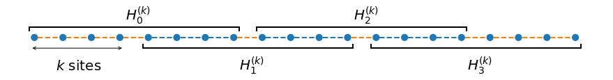
Figure 2: Illustration of where each term $H^{(k)}_{j}$ acts, at $N=20$ and $k=4$. The blue dots represent sites, and the dashed lines connecting them are bonds (interactions) $h_{i}$. The blue bonds are counted twice in the sum $H^{(k)}$, while the orange ones are only included once. This split is used to find the inequality (4.12).

The residual terms in the parentheses on the last line are non-negative operators and so we have

$$2H_{n}\geq H^{(k)}.$$ (4.9)

At any finite $k$, an individual term $H^{(k)}_{j}$ has a finite number of eigenvalues, and therefore a finite spectral gap, which we will call $\gamma_{k}$. Since all $H^{(k)}_{j}$ have the same spectrum regardless of $j$, this value $\gamma_{k}$ will not depend on $j$. Moreover, by frustration-freeness $H^{(k)}_{j}$ has a nontrivial kernel, and its lowest eigenvalue is zero. Therefore we can write

$$H^{(k)}_{j}\geq\gamma_{k}\cdot P^{(k)}_{j}$$ (4.10)

where $P^{(k)}_{j}$ is the projector onto the range of $H^{(k)}_{j}$. Summing over $j$, we obtain

$$H^{(k)}=\sum_{j=0}^{a-2}H^{(k)}_{j}\geq\gamma_{k}S^{(k)},\qquad S^{(k)}=\sum_{j=0}^{a-2}P^{(k)}_{j}.$$ (4.11)

Combining this with the previous result (4.9) we get

$$H_{n}\geq{1\over 2}H^{(k)}\geq{\gamma_{k}\over 2}\cdot S^{(k)}$$ (4.12)

From frustration-freeness we know that the kernel of a sum of projectors $h_{i}$ consists precisely of the states that are annihilated simultaneously by all terms. Since $H_{n}$ and $H^{(k)}$ consist of the same projectors $h_{i}$ (they only have different prefactors), we see that their kernels must be identical. Moreover, $H^{(k)}$ and $S^{(k)}$ have identical kernels by definition of the terms $P_{j}^{(k)}$. Together with the inequality (4.12), we find an ordering between gaps:

$$\gamma(H_{n})\geq{1\over 2}\cdot\gamma(H^{(k)})\geq{\gamma_{k}\over 2}\cdot\gamma(S^{(k)})$$ (4.13)

and it suffices to bound the RHS term from below. To do so, we square $S^{(k)}$,

$$\Big{(}S^{(k)}\Big{)}^{2}=\sum_{j=0}^{a-2}\Big{(}P^{(k)}_{j}\Big{)}^{2}+\sum_{j=1}^{a-2}\sum_{l=0}^{j-1}\{P^{(k)}_{j},P^{(k)}_{l}\}$$ (4.14)

where $\{A,B\}$ denotes the anticommutator of operators $A$ and $B$. Note that since each $P^{(k)}_{j}$ is a projector, we have $\Big{(}P^{(k)}_{j}\Big{)}^{2}=P^{(k)}_{j}$ and $P^{(k)}_{l}P^{(k)}_{j}\geq 0$ if $|j-l|\geq 2$. Hence,

$$\Big{(}S^{(k)}\Big{)}^{2} \geq S^{(k)}+\sum_{j=0}^{a-3}\{P^{(k)}_{j},P^{(k)}_{j+1}\}$$ (4.15)

For the remaining anticommutators we use [FNW92, Lemma 6.3], which gives

$$\{P^{(k)}_{j},P^{(k)}_{j+1}\}\geq-(P^{(k)}_{j}+P^{(k)}_{j+1})\cdot\|\big{(}P^{(k)}_{j+1}\big{)}^{\perp}\big{(}P^{(k)}_{j}\big{)}^{\perp}-\big{(}P^{(k)}_{j}\big{)}^{\perp}\wedge\big{(}P^{(k)}_{j+1}\big{)}^{\perp}\|$$ (4.16)

By translation invariance, the operator norm does not depend on $j$, so we can focus on

$$z_{k}\equiv\|\big{(}P^{(k)}_{1}\big{)}^{\perp}\big{(}P^{(k)}_{0}\big{)}^{\perp}-\big{(}P^{(k)}_{0}\big{)}^{\perp}\wedge\big{(}P^{(k)}_{1}\big{)}^{\perp}\|$$ (4.17)

Summing over $j$, we get

$$\sum_{j=0}^{a-3}\{P^{(k)}_{j+1},P^{(k)}_{j}\}\geq\left(-z_{k}\right)\cdot\left(\sum_{j=0}^{a-3}\big{(}P^{(k)}_{j}+P^{(k)}_{j+1}\big{)}\right)$$ (4.18)

The sum on the RHS is almost twice $S^{(k)}$:

$$\sum_{j=0}^{a-3}\big{(}P^{(k)}_{j}+P^{(k)}_{j+1}\big{)}=2\cdot\sum_{j=0}^{a-2}P^{(k)}_{j}-\left(P^{(k)}_{0}+P^{(k)}_{a-2}\right)\leq 2\cdot\sum_{j=0}^{a-2}P^{(k)}_{j}=2\cdot S^{(k)}$$ (4.19)

Together with $z_{k}\geq 0$, we get from (4.18) that

$$\sum_{j=0}^{a-3}\{P^{(k)}_{j+1},P^{(k)}_{j}\}\geq\left(-2z_{k}\right)\cdot S^{(k)}$$ (4.20)

so that looking back to the square of $S^{(k)}$ we have

$$\Big{(}S^{(k)}\Big{)}^{2}\geq(1-2z_{k})\cdot S^{(k)}$$ (4.21)

As $S^{(k)}$ is a non-negative operator with nontrivial kernel, this gives a lower bound on the gap, $\gamma(S^{(k)})\geq(1-2z_{k})$, which translates into an $n-$independent lower bound on the gap of the original Hamiltonian $H_{n}$:

$$\gamma(H_{n})\geq{\gamma_{k}\over 2}\cdot\gamma(S^{(k)})\geq\gamma_{k}\cdot\left({1\over 2}-z_{k}\right)$$ (4.22)

Since $P^{(k)}_{j}$ projected onto the range of $H^{(k)}_{j}$ by definition, we see that $\big{(}P^{(k)}_{j}\big{)}^{\perp}$ is the ground space projector for sites $jk+1$ through $(j+2)k$, which we will denote by $G_{[jk+1,(j+2)k]}$. In this notation we have

$$\big{(}P^{(k)}_{0}\big{)}^{\perp}=G_{[1,2k]}\qquad\big{(}P^{(k)}_{1}\big{)}^{\perp}=G_{[k+1,3k]}\qquad\big{(}P^{(k)}_{0}\big{)}^{\perp}\wedge\big{(}P^{(k)}_{1}\big{)}^{\perp}=G_{[1,3k]}$$ (4.23)

where the last identity follows from frustration-freeness. The necessary condition, then, is that for some $k$ we have

$$z_{k}=\|G_{[k+1,3k]}G_{[1,2k]}-G_{[1,3k]}\|<{1\over 2}$$ (4.24)

completing the proof of Theorem 4.3. ∎

In the following subsections, we consider the finite-size criterion for open Motzkin chains and reformulate in a convenient way for our later purposes.

4.2 Relations between Motzkin ground states on different subchains

In view of Lemma 4.4, we are led to consider several different segments of Motzkin spin chains, so it will be useful to have a label to keep track of the segment under discussion. For any such segment $S$, we let $G^{S}_{p,q}$ be the equivalence class defined above, i.e., the set of all walks on segment $S$, with $(p,q)$ unbalanced steps. When the segment $S$ under discussion is clear from the context, we occasionally drop the $S$ label.

It will also be useful to consider the unnormalized ground states.

Definition 4.5.

For a spin chain segment $S$, we will denote by $|{UGS^{S}_{p,q}}\rangle$ the unnormalized ground state of the Hamiltonian corresponding to $S$, i.e. the state which is the area-weighted sum of all walks in $G^{S}_{p,q}$:

$$|{UGS^{S}_{p,q}}\rangle=\sum_{w\in G^{S}_{p,q}}t^{A(w)}|{w}\rangle$$ (4.25)

with the following relation to the normalized version

$$|{GS^{S}_{p,q}}\rangle={|{UGS^{S}_{p,q}}\rangle\over\||{UGS^{S}_{p,q}}\rangle\|}={1\over\sqrt{N_{p,q}^{S}}}\cdot\sum_{w\in G^{S}_{p,q}}t^{A(w)}|{w}\rangle$$ (4.26)

where the normalization factor $N_{p,q}^{S}$ is

$$N_{p,q}^{S}=\sum_{w\in G^{S}_{p,q}}t^{2A(w)}$$ (4.27)

Here, we state and prove two other useful properties of ground states, and ground space projectors:

Notation 4.6.

Given a chain segment $S$ and a subset of it $T\subset S$, we denote by $G_{T}$ the ground space projector on $T$. If acting on states living in the Hilbert space associated with $S$ (and $T$ is a proper subset of $S$), we will understand that the operator $G_{T}$ acts as the identity on $\mathcal{H}_{S\setminus T}$, a shorthand for $G_{T}\otimes I_{S\setminus T}$.

Proposition 4.7 (Overlap properties).

For any $S,T$ as above, the ground space projector $G_{T}$, when viewed as acting on the Hilbert space $\mathcal{H}_{T}$, is diagonal in the basis of states with definite numbers of unbalanced steps:

$$\forall|{a_{p,q}}\rangle,|{b_{p^{\prime},q^{\prime}}}\rangle\in\mathcal{H}_{T}\quad\quad\quad\quad(p\neq p^{\prime}\text{ or }q\neq q^{\prime})\quad\implies\quad\langle{b_{p^{\prime},q^{\prime}}}|{G_{T}}|{a_{p,q}}\rangle=0$$ (4.28)

Furthermore, the above holds true even when $G_{T}$ is seen as acting on the Hilbert space $\mathcal{H}_{S}$ associated with the wider segment $S$:

$$\forall|{a_{p,q}}\rangle,|{b_{p^{\prime},q^{\prime}}}\rangle\in\mathcal{H}_{S}\quad\quad\quad\quad(p\neq p^{\prime}\text{ or }q\neq q^{\prime})\quad\implies\quad\langle{b_{p^{\prime},q^{\prime}}}|{G_{T}}|{a_{p,q}}\rangle=0$$ (4.29)

Proof of Proposition 4.7.

We will begin by proving the first claim. The proof of Theorem 2.4 implies that the $|{GS_{p,q}^{T}}\rangle$ form an orthonormal basis for the ground space on $T$. Hence, we can write

$$G_{T}=\sum_{r,s}|{GS_{r,s}^{T}}\rangle\langle{GS_{r,s}^{T}}|$$ (4.30)

with the sum running over all possible $p,q$ consistent with $T$ (i.e. $p+q\leq|T|$). Since $|{a_{p,q}}\rangle$ contains only walks in $G^{T}_{p,q}$, it will only have nonvanishing overlap with $|{GS_{p,q}^{T}}\rangle$ (same argument as in the proof of Theorem 2.4), and so

$$G_{T}|{a_{p,q}}\rangle=\left(\sum_{r,s}|{GS_{r,s}^{T}}\rangle\langle{GS_{r,s}^{T}}|\right)|{a_{p,q}}\rangle=|{GS_{p,q}^{T}}\rangle\cdot\langle{GS_{p,q}^{T}}|{a_{p,q}}\rangle$$ (4.31)

Because the RHS is proportional to $|{GS_{p,q}^{T}}\rangle$, it only contains walks in $G^{T}_{p,q}$. Therefore the only possibility for nonvanishing overlap with $|{b_{p^{\prime},q^{\prime}}}\rangle$ is to have both $p=p^{\prime}$ and $q=q^{\prime}$.

The following characterization will be useful for the second part of the proof: since all walks in the composition of $G_{T}|{a_{p,q}}\rangle$ still lie in the equivalence class $G_{p,q}^{T}$, it means that any of them can be transformed, using only local moves, into any walk contributing to the original state $|{a_{p,q}}\rangle$.

For the second claim, working in $\mathcal{H}_{S}$, we again investigate how $G_{T}$ acts on $|{a_{p,q}}\rangle$. For any walk included in $|{a_{p,q}}\rangle$, the projector $G_{T}$ may only change the steps in $T$, since it acts as the identity on $S\setminus T$. We have also seen above that any such change is revertible by local moves. Therefore any walk in $G_{T}|{a_{p,q}}\rangle$ (living on the full segment $S$) can still be transformed, by local moves, into any walk from $|{a_{p,q}}\rangle$. We conclude that $G_{T}$ does not change the equivalence class of walks even when acting on the full $S$, and the claim follows. ∎

4.3 Reformulation of the criterion for Motzkin chains

In this section we reduce the criterion 4.3 to a form better suited for the translation-invariant part $H_{n}^{0}$ of the Motzkin Hamiltonian under discussion (eq. (2.7)). We define a collection of states, indexed by $k$:

Definition 4.8.

By $|{\phi^{(k)}_{p,q}}\rangle$ we mean a state with $(p,q)$ unbalanced steps living in the Hilbert space associated with sites $[1,3k]$. For notational simplicity the $k$ label may be dropped, leaving $|{\phi_{p,q}}\rangle$ as the state.

The main result of this section is the following:

Proposition 4.9.

With the Definitions 4.2 and (4.2) we have,

$$\|G_{[k+1,3k]}E_{k}\|=\sqrt{\sup\limits_{\begin{subarray}{c}p,q\geq 0\\ p+q\leq 3k\end{subarray}}\left(\sup\limits_{\phi_{p,q}\in\operatorname{range}E_{k}}\langle{\phi_{p,q}}|{G_{[k+1,3k]}}|{\phi_{p,q}}\rangle\right)}$$ (4.32)

Proof of Proposition 4.9.

From the definition of the norm,

$$\|G_{[k+1,3k]}E_{k}\|=\sup\limits_{\phi\in\mathcal{H}_{[1,3k]}}\|G_{[k+1,3k]}E_{k}|{\phi}\rangle\|=\sup\limits_{\phi\in\mathcal{H}_{[1,3k]}}\sqrt{\langle{\phi}|{E_{k}G_{[k+1,3k]}G_{[k+1,3k]}E_{k}}|{\phi}\rangle}$$ (4.33)

Since $G_{[k+1,3k]}$ is a projector, it squares to itself, and the above simplifies to

$$\|G_{[k+1,3k]}E_{k}\|=\sup\limits_{\phi\in\mathcal{H}_{[1,3k]}}\sqrt{\langle{\phi}|{E_{k}G_{[k+1,3k]}E_{k}}|{\phi}\rangle}$$ (4.34)

In the above, $\phi$ is a priori an arbitrary state in the Hilbert space $\mathcal{H}_{[1,3k]}$. However, without loss of generality, we can take it to be in the range of $E_{k}$. This is because $\mathcal{H}_{[1,3k]}$ can be written as the direct sum of $\operatorname{range}E_{k}$ and its orthogonal complement. Any part of $|{\phi}\rangle$ in the orthogonal complement gets annihilated by the projector $E_{k}$, without contributing anything to the norm. This means we can take

$$E_{k}|{\phi}\rangle=|{\phi}\rangle\quad\iff\quad G_{[1,2k]}|{\phi}\rangle=|{\phi}\rangle\quad\text{and}\quad G_{[1,3k]}|{\phi}\rangle=0$$ (4.35)

and obtain the norm as

$$\|G_{[k+1,3k]}E_{k}\|=\sup\limits_{\phi\in\operatorname{range}E_{k}}\sqrt{\langle{\phi}|{G_{[k+1,3k]}}|{\phi}\rangle}$$ (4.36)

Since the square root is strictly increasing, we can safely take it out of the supremum to obtain

$$\|G_{[k+1,3k]}E_{k}\|=\sqrt{\sup\limits_{\phi\in\operatorname{range}E_{k}}\langle{\phi}|{G_{[k+1,3k]}}|{\phi}\rangle}$$ (4.37)

As seen in the proof of Proposition 4.7, the ground space projector on any interval $I$ can be written as

$$G^{I}=\sum_{p,q}|{GS^{I}_{p,q}}\rangle\langle{GS^{I}_{p,q}}|$$ (4.38)

Each term selects the component of $|{\phi}\rangle$ with the corresponding number of unbalanced steps. Expanding $|{\phi}\rangle$ in terms of such components, we find

$$|{\phi}\rangle=\sum_{p,q}a_{p,q}|{\phi_{p,q}}\rangle$$ (4.39)

where we assume each $|{\phi_{p,q}}\rangle$ is in the range of $E_{k}$, is normalized, and has $(p,q)$ unbalanced steps. Normalization for $|{\phi}\rangle$ requires

$$1=\langle{\phi}|{\phi}\rangle=\sum_{p,q}|a_{p,q}|^{2}$$ (4.40)

where the second equality above follows from the orthonormality of individual components: for any $p,q,p^{\prime},q^{\prime}$ we have $\langle{\phi_{p,q}}|{\phi_{p^{\prime},q^{\prime}}}\rangle=\delta_{p,p^{\prime}}\cdot\delta_{q,q^{\prime}}$. It follows that

$$\langle{\phi}|{G_{[k+1,3k]}}|{\phi}\rangle=\sum_{p,q,p^{\prime},q^{\prime}}a_{p,q}\cdot a_{p^{\prime},q^{\prime}}^{*}\cdot\langle{\phi_{p^{\prime},q^{\prime}}}|{G_{[k+1,3k]}}|{\phi_{p,q}}\rangle=\sum_{p,q}|a_{p,q}|^{2}\cdot\langle{\phi_{p,q}}|{G_{[k+1,3k]}}|{\phi_{p,q}}\rangle$$ (4.41)

where the second equality follows from $\langle{\phi_{p^{\prime},q^{\prime}}}|{G_{[k+1,3k]}}|{\phi_{p,q}}\rangle=\langle{\phi_{p,q}}|{G_{[k+1,3k]}}|{\phi_{p,q}}\rangle\cdot\delta_{p,p^{\prime}}\cdot\delta_{q,q^{\prime}}$; the ground space projector does not have matrix elements between states with different numbers of unbalanced steps, as shown in Proposition 4.7.

From the normalization condition (4.40), and the fact that $G_{[k+1,3k]}$ is a non-negative operator, we see

$$\langle{\phi}|{G_{[k+1,3k]}}|{\phi}\rangle=\sum_{p,q}|a_{p,q}|^{2}\cdot\langle{\phi_{p,q}}|{G_{[k+1,3k]}}|{\phi_{p,q}}\rangle\leq\sup\limits_{p,q}\langle{\phi_{p,q}}|{G_{[k+1,3k]}}|{\phi_{p,q}}\rangle$$ (4.42)

and the bound can be attained, since there is no constraint on the $a_{p,q}$ coefficients other than normalization. Choosing all of them to be zero, except for the one corresponding to the largest matrix element $\langle{\phi_{p,q}}|{G_{[k+1,3k]}}|{\phi_{p,q}}\rangle$, gives equality in the above. Formally, this means

$$\sup\limits_{\phi\in\operatorname{range}E_{k}}\langle{\phi}|{G_{[k+1,3k]}}|{\phi}\rangle=\sup\limits_{\begin{subarray}{c}p,q\geq 0\\ p+q\leq 3k\end{subarray}}\left(\sup\limits_{\phi_{p,q}\in\operatorname{range}E_{k}}\langle{\phi_{p,q}}|{G_{[k+1,3k]}}|{\phi_{p,q}}\rangle\right)$$ (4.43)

where we’ve made explicit the conditions on $p$ and $q$. At fixed $k$, the length of the full chain is $3k$; the number of unbalanced steps must be non-negative, and also can never be more than the total steps, so $p,q\geq 0$ and $p+q\leq 3k$. We then find that

$$\|G_{[k+1,3k]}E_{k}\|=\sqrt{\sup\limits_{\begin{subarray}{c}p,q\geq 0\\ p+q\leq 3k\end{subarray}}\left(\sup\limits_{\phi_{p,q}\in\operatorname{range}E_{k}}\langle{\phi_{p,q}}|{G_{[k+1,3k]}}|{\phi_{p,q}}\rangle\right)}$$ (4.44)

completing the proof. ∎

5 Analytical verification of the finite-size criterion: overview

The remaining sections will focus on showing the following key asymptotic.

Theorem 5.1 (Key asymptotic).

We have

$$\lim\limits_{k\to\infty}\left(\sup\limits_{\begin{subarray}{c}p,q\geq 0\\ p+q\leq 3k\end{subarray}}\left(\sup\limits_{\phi_{p,q}\in\operatorname{range}E_{k}}\langle{\phi_{p,q}}|{G_{[k+1,3k]}}|{\phi_{p,q}}\rangle\right)\right)=0$$ (5.1)

This asymptotic readily implies Theorem 5.1 and hence the main result.

Proof of Theorem 2.5 assuming Theorem 5.1.

Together with Proposition 4.9, the asymptotic (5.1) implies that

$$\|G_{[k+1,3k]}E_{k}\|\to 0,\qquad k\to\infty.$$

By Lemma 4.4, this implies that there exists a large $k_{0}$ such that Theorem 4.3 applies and yields Theorem 2.5 (which as already seen then gives the main result). ∎

Therefore, the task that will occupy us in the remainder of this work is to prove Theorem 5.1. This turns out to be technically quite challenging and requires several new ideas in the analysis of the Motzkin spin chain to be completed. A special role is played by a suitable notion of approximate ground state projectors introduced in the next section. We develop a detailed description of the behavior of these approximate ground states under composition and decomposition in different physical regimes (low-imbalance versus high-imbalance). We also derive precise control on their combinatorial normalization coefficients based on rather technical estimates for a spatially inhomogeneous 1D diffusion equation. It would be interesting if this refined understanding of the open-chain ground states could be useful to study other physical properties of Motzkin spin chains.

Proof strategy for Theorem 5.1

First, notice that we can understand the quantity on the LHS of (5.1) as measuring the ‘delocalization’ of possible excitations in the model: we look at states $|{\phi}\rangle$ on the full chain which are excited (orthogonal to the full-chain ground space), but their components on the first two-thirds of the chain are local ground states. We then ask how much these states can overlap with the ground space on the last two-thirds of the chain, and we aim to show that the answer is almost not at all. Intuitively speaking, we have to exclude the possibility that there exists some excited state on the full chain which is very close to ground states on the first two-thirds and also the last two-thirds of the chain. This latter situation would require some form of non-localized excitation.

The main technical difficulty arises because of the quadratic ground state degeneracy described in Theorem 4.3, which is the price to pay for removing the boundary projectors. This means that we must consider ground states with various $p$- and $q$-values, not only on the initial chain, but also (and this is the crux of the matter) when dividing the chain into subsegments. It is therefore imperative that we develop a simpler-to-work-with effective description, we call these approximate ground states.

Our notion of approximate ground states differs based on two main categories: states with many unbalanced steps or few ones (called high-imbalance and low-imbalance respectively). The simpler case is when there are many unbalanced steps of at least one type (up or down), i.e. more than $(1+c)\cdot k$ such steps, for some $c>0$. Then, because of the area weighting in the ground state, the outermost $k$ unbalanced steps will tend to accumulate in the corresponding outermost third of the chain. The reason is that the presence of any balanced step in the outermost third carries, in comparison with the lowest-area walk, an additional-area cost that is of order $k$. Therefore, at large $k$, a ground state on the full chain will overwhelmingly contain only unbalanced steps in one of its thirds, and can therefore be approximated by a convenient product state. This approximation is made precise in Section 7, and its application to obtain the desired bound is outlined in Section 8.2.

On the other hand, for the case with few unbalanced steps on both sides, our approximation will rely on a Schmidt decomposition of the exact ground state, followed by a rigorous proof that most of the terms can be ignored in the large $k$ limit. The intuition is that, if we divide the full chain into three segments, all of which have length on the order of $k$, it is exponentially unlikely to have, in the composition of the full ground state, walks which do not reach the zero-height level in all three such segments separately. This can be understood, again, due to the area cost of such an extraordinary walk being on the order of $k$ larger than the minimum-area walk. At large enough $k$, the exponential weighting will suppress all such extraordinary walks. The specific details and proof of this low-imbalance approximation are presented in Section 6. Combining it with some technical properties of the normalizations for our states (Section 9, which relies on the diffusion analysis of Appendix A), we find that the bound also holds for few unbalanced steps (Sections 8.3 and 10).

In the end, we combine all of these results and conclude the central asymptotic formula (5.1).

6 Low-imbalance approximations

Throughout this and the following sections, we will approximate ground states and $|{\phi_{p,q}}\rangle$ states by combinatorially simpler objects.

Definition 6.1.

Given two collections of states indexed by $k$, call them $\{|{a^{(k)}}\rangle\}$ and $\{|{b^{(k)}}\rangle\}$, we will say that the latter superpolynomially approximates the former if

$$\forall n\in\mathbb{N}:\qquad\qquad\lim\limits_{k\to\infty}\left[k^{n}\cdot\Big{(}1-|\langle{a^{(k)}}|{b^{(k)}}\rangle|^{2}\Big{)}\right]=0$$ (6.1)

The ground states of our Hamiltonian can be divided into two categories: those with small, and respectively large, numbers of unbalanced steps. This classification is relative to a division of the spin chain into subsegments, and will be made precise below. In this section, we find superpolynomial approximations for the low-imbalance ground states of our Hamiltonian. The next section will similarly treat the high-imbalance states. We start with some necessary assumptions and definitions:

Assumption 6.2.

Let $f_{1}$, $f_{2}>0$ be two given constants; fix a small number $b$ with $0<b<f_{1},f_{2}$. We also fix two other constants $a_{1}$, $a_{2}$ such that $0<a_{1}<f_{1}-b$ and $0<a_{2}<f_{2}-b$.

Although it is irrelevant in this section, the following condition on $b$ will later be essential: we shall impose $b<{1\over 4\beta}$, where $\beta>0$ is the parameter appearing in Theorem A.2. Note that $\beta$ depends only on the value of $t$, so we can indeed take it to be fixed once $t$ is specified.

Notation 6.3.

We will consider a family of spin chain segments indexed by $k$, where at each $k$ the corresponding segment contains $(f_{1}+f_{2})k$ sites. We will view such a segment as composed from two parts: the left one (L) of length $f_{1}k$, and the right (R) one, with length $f_{2}k$.

Definition 6.4.

For every segment in Notation 6.3 we define an approximate ground state with $(p,q)$ unbalanced steps, living in the Hilbert space associated with the entire segment $L\cup R$, as

$$|{ATGS_{p,q}}\rangle={1\over\sqrt{ATN_{p,q}}}\sum_{r<bk}|{UGS^{L}_{p,r}}\rangle|{UGS^{R}_{r,q}}\rangle$$ (6.2)

where the $k$ label was suppressed for simplicity in the naming of all states, and the normalization factor is defined in the natural way:

$$ATN_{p,q}=\sum_{r<bk}N^{L}_{p,r}\cdot N^{R}_{r,q}$$ (6.3)

We are now ready to state the result of this section:

Lemma 6.5.

With the Definitions 6.1, 6.4 Assumption 6.2, and Notation 6.3 from above, we have that, for all $p<a_{1}k$ and $q<a_{2}k$, the truncated approximate ground states of eq. (6.2) superpolynomially approximate the true ground states on the corresponding segments:

$$\forall n\in\mathbb{N}:\quad\quad\quad\quad\lim\limits_{k\to\infty}\left[k^{n}\cdot\sup\limits_{\begin{subarray}{c}p<a_{1}k\\ q<a_{2}k\end{subarray}}\Big{(}1-|\langle{GS_{p,q}}|{ATGS_{p,q}}\rangle|^{2}\Big{)}\right]=0$$ (6.4)

We begin with a discussion of the structure of ground states in this low-imbalance regime, followed by a two-part proof of Lemma 6.5.

6.1 Splitting the ground states

As discussed in Section 3.1, the ground state with ($p,q$) unbalanced steps, corresponding to a chain segment $S$, is the area-weighted superposition of all walks in $G_{p,q}^{S}$. Since walks are defined to have the minimal area consistent with non-negativity, they must reach zero height in at least one point. If this is the case, the starting and ending heights for a walk $w$ with $(p,q)$ unbalanced steps must be $p$ and $q$ respectively, as can be seen by performing local moves that transform $w$ into $g_{p,q}$. On the other hand, if we are given a walk that is not minimal, we can “minimize” it by shifting it down by an appropriate amount (Fig. 3).

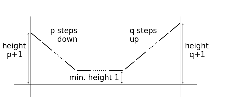
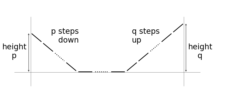
Figure 3: Walks that do not reach zero height at any point (a) can be “minimized” by shifting them down, until they do so (b). In this latter form, the starting and ending heights are equal to the numbers of unbalanced down and up steps, respectively.

We will view $S$ as being divided into two parts $L$ and $R$, as in Notation 6.3. In this case, a valid walk can either reach zero height in only one of these subsegments, or in both. Formally, we can write $G^{S}_{p,q}$ as the disjoint union of the following: (also see Fig. 4)

• $H^{S;\;LR}_{p,q}$, containing the walks which reach zero height both in the $L$ and $R$ segments.

• $H^{S;\;L}_{p,q}$, containing the walks which reach zero height in the $L$ segment, but not in $R$.

• $H^{S;\;R}_{p,q}$, containing the walks which reach zero height in the $R$ segment, but not in $L$.

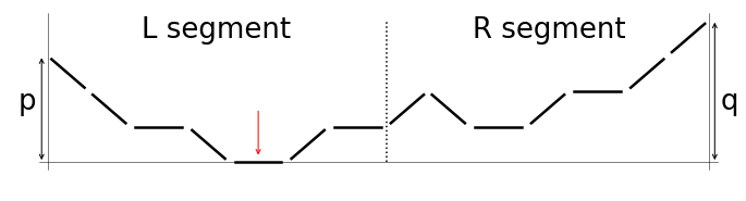
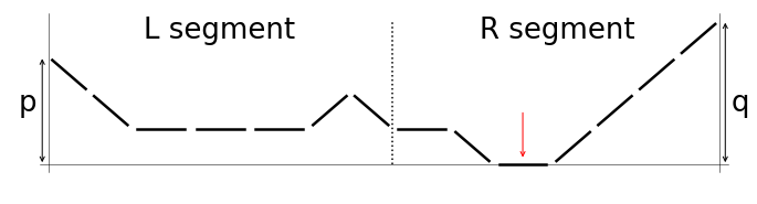
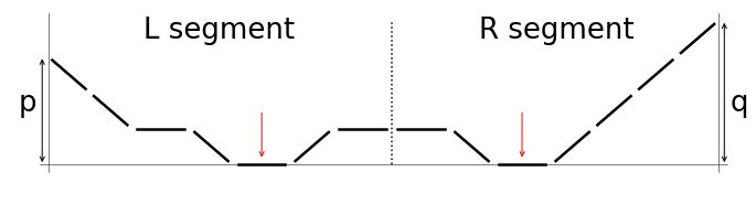
Figure 4: Typical walks belonging to the subcollections $H^{L}_{p,q}$ (a), $H^{R}_{p,q}$ (b), and $H^{LR}_{p,q}$ (c). The red arrows indicate the regions of zero height that determine this classification. The three subcollections are used for the ground state decomposition in eq. (6.5).

Notation 6.6.

Throughout the rest of the section, the segment $S$ under consideration will be understood to be as in Notation 6.3, and so its corresponding label will be omitted for simplicity. The three classes above will be denoted by $H^{LR}_{p,q}$, $H^{L}_{p,q}$, and $H^{R}_{p,q}$ respectively.

Using Definition 4.5, write the (unnormalized) exact ground state as

$$|{UGS_{p,q}}\rangle=\sum_{w\in H^{LR}_{p,q}}t^{A(w)}|{w}\rangle+\sum_{w\in H^{L}_{p,q}}t^{A(w)}|{w}\rangle+\sum_{w\in H^{R}_{p,q}}t^{A(w)}|{w}\rangle$$ (6.5)

with the corresponding normalization factor

$$N_{p,q}=\langle{UGS_{p,q}}|{UGS_{p,q}}\rangle=\sum_{w\in H^{LR}_{p,q}}t^{2A(w)}+\sum_{w\in H^{L}_{p,q}}t^{2A(w)}+\sum_{w\in H^{R}_{p,q}}t^{2A(w)}$$ (6.6)

and the normalized ground state

$$|{GS_{p,q}}\rangle={1\over\sqrt{N_{p,q}}}\;|{UGS_{p,q}}\rangle={1\over\sqrt{N_{p,q}}}\;\left(\sum_{w\in H^{LR}_{p,q}}t^{A(w)}|{w}\rangle+\sum_{w\in H^{L}_{p,q}}t^{A(w)}|{w}\rangle+\sum_{w\in H^{R}_{p,q}}t^{A(w)}|{w}\rangle\right)$$ (6.7)

6.2 The first approximation

We will first show that, in the low$-p$ and low$-q$ regime (more precisely, we require $p<a_{1}k$ and $q<a_{2}k$), the first term in the RHS of eq. (6.6) dominates the other two, and we find an approximate ground state which includes only walks in $H^{LR}_{p,q}$ (see Lemma 6.8 below).

Definition 6.7.

For every spin chain of Notation 6.3 we define (suppressing the $k$ index) an approximate ground state on $L\cup R$:

$$|{AGS_{p,q}}\rangle={1\over\sqrt{AN_{p,q}}}\sum_{w\in H^{LR}_{p,q}}t^{A(w)}|{w}\rangle$$ (6.8)

including only the walks that reach zero height in both $L$ and $R$. Here $AN_{p,q}$ is the corresponding approximate normalization factor

$$AN_{p,q}=\sum_{w\in H^{LR}_{p,q}}t^{2A(w)}$$ (6.9)

The precise formulation of the claim from above is:

Lemma 6.8.

Under Assumption 6.2, Notation 6.3 and with the Definitions 6.1, 6.7 we have that the $|{AGS_{p,q}}\rangle$ superpolynomially approximate the true ground states $|{GS_{p,q}}\rangle$:

$$\forall n\in\mathbb{N}:\quad\quad\quad\quad\lim\limits_{k\to\infty}\left[k^{n}\cdot\sup\limits_{\begin{subarray}{c}p<a_{1}k\\ q<a_{2}k\end{subarray}}\Big{(}1-|\langle{GS_{p,q}}|{AGS_{p,q}}\rangle|^{2}\Big{)}\right]=0$$ (6.10)

Proof of Lemma 6.8.

From Definition 6.7, see that the overlap between the approximate and exact ground states is given only by the terms in $H^{LR}_{p,q}$, and it is equal to

$$\langle{GS_{p,q}}|{AGS_{p,q}}\rangle={\sum_{w\in H^{LR}_{p,q}}t^{2A(w)}\over\sqrt{N_{p,q}\cdot AN_{p,q}}}={AN_{p,q}\over\sqrt{N_{p,q}\cdot AN_{p,q}}}=\sqrt{AN_{p,q}\over N_{p,q}}$$ (6.11)

Guided by eq. (6.6) make the notations $N^{L}_{p,q}\equiv\sum_{w\in H^{L}_{p,q}}t^{2A(w)}$ and $N^{R}_{p,q}\equiv\sum_{w\in H^{R}_{p,q}}t^{2A(w)}$, such that we get $N_{p,q}=AN_{p,q}+N^{L}_{p,q}+N^{R}_{p,q}$ and the equation above becomes

$$\langle{GS_{p,q}}|{AGS_{p,q}}\rangle=\sqrt{N_{p,q}-N^{L}_{p,q}-N^{R}_{p,q}\over N_{p,q}}=\sqrt{1-{N^{L}_{p,q}\over N_{p,q}}-{N^{R}_{p,q}\over N_{p,q}}}$$ (6.12)

so that

$$\quad 1-|\langle{GS_{p,q}}|{AGS_{p,q}}\rangle|^{2}={N^{L}_{p,q}\over N_{p,q}}+{N^{R}_{p,q}\over N_{p,q}}$$ (6.13)

and since both ${N^{L}_{p,q}\over N_{p,q}}$ and ${N^{R}_{p,q}\over N_{p,q}}$ are positive quantities by definition, it suffices to show that they separately vanish fast enough, under the given conditions.

We will focus on the ${N^{L}_{p,q}\over N_{p,q}}$ term, and the argument for the other one will be analogous. The normalization factor $N^{L}_{p,q}$ contains contributions from walks that only reach zero height in the leftmost interval, but not in the rightmost one. The minimum height they reach within the right interval must be a positive integer, and we can classify the walks by this minimum height.

Definition 6.9.

Let $H^{L,h}_{p,q}$ be the subcollection of walks that reach zero height in $L$, but only reach minimum height $h>0$ in $R$. Also let $N^{L,h}_{p,q}$ be the contribution to normalization due to walks in $H^{L,h}_{p,q}$:

$$N^{L,h}_{p,q}=\sum_{w\in H^{L,h}_{p,q}}t^{2A(w)}$$ (6.14)

We see that $H^{L}_{p,q}$ is the disjoint union of $H^{L,1}_{p,q}$, $H^{L,2}_{p,q}$ and so on. Since all walks under discussion must end at height $q$ due to the condition on unbalanced steps, we see that their minimum height within $R$ cannot be more than $q$. Then, the $H^{L,h}_{p,q}$ for all $h>q$ are empty and one can express $H^{L}_{p,q}$ as the disjoint union of the $H^{L,h}_{p,q}$ for $h\in\{1,2,\dots q\}$ . The normalization factor $N^{L}_{p,q}$ can be written as the sum

$$N^{L}_{p,q}=\sum_{w\in H^{L}_{p,q}}t^{2A(w)}=\sum_{h=1}^{q}\sum_{w\in H^{L,h}_{p,q}}t^{2A(w)}=\sum_{h=1}^{q}N^{L,h}_{p,q}$$ (6.15)

The intuition here is that walks with larger $h$ must enclose correspondingly large areas (for example, at least $h$ times the length of $R$, guaranteed by the minimum height condition). Since the size of $R$ is $f_{2}k$ and $t<1$, this translates into exponentially small normalization factors $t^{2A(w)}$ when $k$ is large: $AN_{p,q}\gg N^{L,1}_{p,q}\gg N^{L,2}_{p,q}\gg\dots$; to formalize this, begin by considering the relation between $AN_{p,q}$ and $N^{L,1}_{p,q}$:

Proposition 6.10.

The ratio of $N^{L,1}_{p,q}$ to $AN_{p,q}$ (where both quantites are understood to implicitly depend on $k$) vanishes faster than polynomially in $k$:

$$\forall n\in\mathbb{N}:\qquad\qquad\lim\limits_{k\to\infty}\left[k^{n}\cdot\sup\limits_{\begin{subarray}{c}p<a_{1}k\\ q<a_{2}k\end{subarray}}\left({N^{L,1}_{p,q}\over AN_{p,q}}\right)\right]=0$$ (6.16)

Proof of Proposition 6.10.

The goal is to formalize the intuition that walks in $H^{L,1}_{p,q}$ will enclose larger areas than those belonging to $H^{LR}_{p,q}$, which gives them exponentially smaller weights, because $t<1$. However, there is not a one-to-one correspondence between walks in $H^{L,1}_{p,q}$ and those in $H^{LR}_{p,q}$, and in fact the numerator $N^{L,1}_{p,q}$ may contain significantly more distinct terms than the denominator $AN_{p,q}$.

The strategy is to construct a mapping $H^{L,1}_{p,q}\to H^{LR}_{p,q}$ with the following two properties:

• It maps any walk in $H^{L,1}_{p,q}$ to one in $H^{LR}_{p,q}$, with area smaller by at least a linear function of $k$.

• The number of different walks from the domain that get mapped to the same target in $H^{LR}_{p,q}$ is at most polynomial in $k$.

Once such a mapping is constructed, the ratio $N^{L,1}_{p,q}/AN_{p,q}$ is bounded above by a polynomial times an exponential in $k$, which will vanish even if multiplied by an additional $k^{n}$ factor. To construct the map, first establish an important property of unbalanced steps:

Proposition 6.11.

When counting unbalanced up-steps from left to right in a minimized walk (cf. Fig. 3), the $i^{\text{th}}$ such step goes from height $i-1$ to $i$. Similarly, the $j^{\text{th}}$ unbalanced down step goes from height $p-j+1$ to $p-j$.

Proof of Proposition 6.11.

An up-step $y_{u}$, going from height $z$ to $z+1$ within a walk, is balanced if there exists a down-step to its right, which goes between $z+1$ and $z$. We will call the nearest such down-step $y_{d}$ (i.e. the leftmost one that is still to the right of $y_{u}$) its balancing partner. A step is unbalanced if it has no such balancing partner.

It follows that, if we have an unbalanced up step $y$ going between $z$ and $z+1$, there is no partner to its right that goes back down to height $z$ or lower. The entire portion of the walk to the right of $y$ is only situated at heights $z+1$ or higher. Moreover, since the step $y$ is assumed to end at height $z+1$, the portion to its right must start at this height; then, the minimum height of this portion is precisely $z+1$.

As a consequence, for any $z\in\{1,2,\dots q-1\}$ there is an unique unbalanced up step going between $z$ and $z+1$. (To see why, assume the contrary and take two such distinct steps; the rightmost one has an end at height $z$, contradicting the conclusion of the previous paragraph). The first statement of Proposition 6.11 follows, and an analogous argument also proves the second claim. ∎

For a given value of $h$, take any walk $w\in H^{L,h}_{p,q}$, and let $s_{i}$ be the $i^{\text{th}}$ unbalanced up-step of $w$. The $s_{i}$ are constrained to lie in $L$ or $R$ respectively, based on the value of $i$, as follows:

Proposition 6.12.

The first $h$ unbalanced steps $\{s_{1},s_{2},\dots s_{h}\}$ are located in the $L$ subsegment, and the other ones $\{s_{h+1},\dots s_{q}\}$ are in R.

Proof of Proposition 6.12.

The portion of $w$ that lies in the $R$ segment reaches minimum height $h$ by assumption, while from Proposition 6.11 we know that $s_{h}$ goes between heights $h-1$ and $h$. Therefore $s_{h}$ cannot be in $R$, and neither can all the previous unblanced up steps $\{s_{1},s_{2},\dots s_{h-1}\}$; all of them must be found in $L$. On the other hand, from the proof of the same Proposition, we find that the portion of $w$ to the right of $s_{h+1}$ only lies at heights $h+1$ and above. This portion cannot contain all the steps in $R$, since by assumption some of them reach height $h$. Therefore $s_{h+1}$ must be contained in $R$. All other unbalanced up-steps $\{s_{h+2},\dots s_{q}\}$ are to the right of $s_{h+1}$, so also in $R$. We conclude that $w$ has $h$ unbalanced up steps in $L$, and the other $q-h$ in $R$. ∎

Note: The result above, with a general value of $h$, is useful when bounding the ratio $N^{L,h}_{p,q}/N^{L,h-1}_{p,q}$. For the current argument, it suffices to use the $h=1$ result, which says that walks in $H^{L,1}_{p,q}$ have a single unbalanced up step in $L$, and the others in $R$.

To describe the mapping process, consider an arbitrary walk $w\in H^{L,1}_{p,q}$, and let $b_{1}$ be its rightmost balanced step. We establish that $b_{1}$ is separated from $s_{1}$ by a number of steps that grows linearly with $k$:

Proposition 6.13.

The step $b_{1}$ is located in the $R$ segment, and the distance $d(s_{1},b_{1})$ between the $s_{1}$ and $b_{1}$ steps obeys the following:

$$d(s_{1},b_{1})>f_{2}k-q>(f_{2}-a_{2})k$$ (6.17)

Proof of Proposition 6.13.

There are $f_{2}k$ total steps in $R$ but, by Proposition 6.12, only $q-1$ unbalanced ones. Since we have $q<a_{2}k<f_{2}k$ by assumption, there must also exist balanced steps in $R$. In particular, since it is the rightmost one, $b_{1}$ is in $R$. As there are only $q-1$ unbalanced up steps in that subsegment, $b_{1}$ must be at most $q-1$ positions away from the rightmost end of the chain. Meanwhile, $s_{1}$ is in $L$, so it is at least the size of $R$ (namely, $f_{2}k$) positions away from the right end of the chain. Therefore the distance between $s_{1}$ and $b_{1}$ is bounded below by $(f_{2}-a_{2})k$, as claimed. ∎

Since any balanced up step has a down partner to its right, which is also balanced itself, the last balanced step ($b_{1}$) cannot be up; it may only be flat or down. See Fig. 5 for an example.

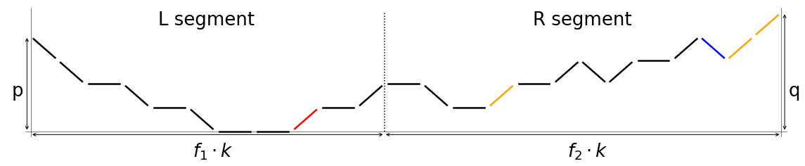
Figure 5: Typical walk in $H^{L,1}_{p,q}$. The leftmost unbalanced up step $s_{1}$ is in the $L$ segment, colored in red. The other unbalanced up-steps are in orange. The rightmost balanced step $b_{1}$ is blue.

For the mapping, we will need $b_{1}$ to be flat. If it is down instead, find its flattening partner $b_{2}$ (which must be an up-step to its left), and replace them both by flat steps (Fig. 6). This procedure does not affect the number of unbalanced steps that the walk $w$ has, nor its minimum height in the $R$ segment, and therefore all the previous conclusions are still valid.

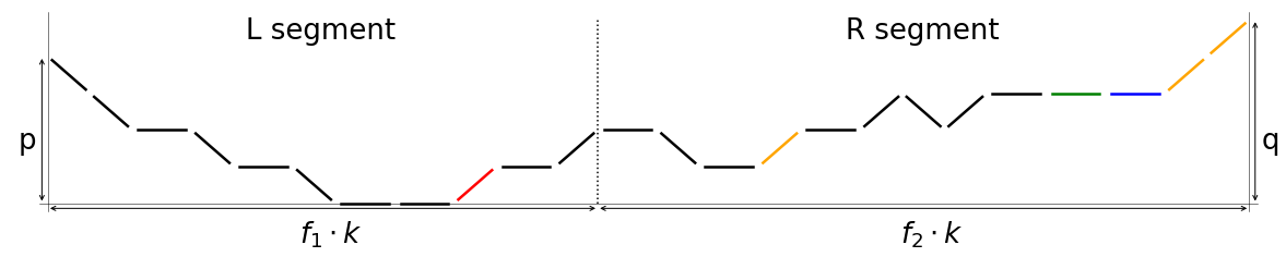
Figure 6: The walk from Figure 5, with the rightmost balanced step $b_{1}$ (which was up) and its partner $b_{2}$ (which came right before it) flattened as discussed in the paragraph above. The last balanced step is still $b_{1}$. The flattened partner $b_{2}$ is shown in green.

Observe that all the points where the walk $w$ reaches height 1 must either belong to $b_{1}$ or be to its left. This is because all the steps to the right of $b_{1}$ are ascending by assumption, so they will never return to the height where $b_{1}$ is located. This height must be at least 1 by the assumption that $w\in H^{L,1}_{p,q}$.

The main operation is exchanging the steps $s_{1}$ and $b_{1}$. Since $s_{1}$ was up but $b_{1}$ was flat, this swap will lower the height of the portion between them by one unit. Everything else will remain at the same level (see Fig. 7). Call the resulting walk $w^{\prime}$.

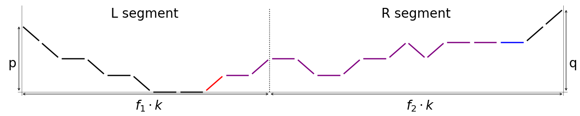
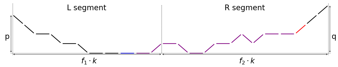
Figure 7: Before (a) and after (b) the exchange of $s_{1}$ with $b_{1}$. Through this swap, the purple section gets shifted down by one unit of height, without its component steps being modified. The rest of the walk is unaffected. The enclosed area in (b) is significantly smaller than in (a), so the contribution of the new walk $w^{\prime}$ to the ground state normalization factor is larger than that of the old walk $w$.

Proposition 6.14.

The walk $w^{\prime}$ obtained through the process described above belongs to the collection $H_{p,q}^{LR}$.

Proof of Proposition 6.14.

First we establish that $w^{\prime}$ still has the same numbers $(p,q)$ of unbalanced steps. Since for a minimized walk these are equal to the starting and ending heights, and the endpoints of our walk are not affected by the swap, it suffices to argue that $w^{\prime}$ is still minimized. Namely, we argue that the minimal overall height of $w^{\prime}$ is still zero. This is true because the section that got shifted down was to the right of $s_{1}$, so by Proposition 6.11 it had a minimum height of 1 before the shift. After the shift, this minimum height will be reduced by one unit, to zero. The rest of the walk was not changed, and since $w$ was minimized, no part of it went below zero height. Therefore the overall minimal height of $w^{\prime}$ is also zero, so $w^{\prime}$ is indeed minimized.

The second property that we must check is that $w^{\prime}$ reaches zero height within both the $L$ and $R$ segments. It has been argued above that all the points where $w$ reached a height of 1 must have been to the left of $b_{1}$. At least one such point must have been in $R$ by the assumption $w\in H^{L,1}_{p,q}$, so in particular it was to the right of $s_{1}$, i.e. in the section that got shifted down. After the swap it is found at zero height, and so $w^{\prime}$ now reaches zero height within $R$. On the other hand, the left endpoint of $s_{1}$, which lies in $L$, had been at zero height by Proposition 6.11. That point is not affected by the swap, so $w^{\prime}$ also reaches zero height in $L$ and the proof is complete. ∎

Note that it is straightforward to generalize the above to a mapping $H^{L,h+1}_{p,q}\to H^{L,h}_{p,q}$. Locate the rightmost balanced step, flatten it (along with its partner) if required, and then swap it with $s_{1}$.

Now we turn to analyzing the area of $w^{\prime}$. The portion that got lowered by one unit of height was seen in Prop. 6.13 to have length larger than $(f_{2}-a_{2})k$, and so

$$A(w^{\prime})<A(w)-(f_{2}-a_{2})k$$ (6.18)

Observe that if the extra flattening step is performed before the swap, this only gives a further reduction of the area (Fig. 6) and so the bound above still holds true. In any case, the described swap procedure only changes two (if no flattening is needed) or three (including flattening) steps of the original walk $w$ (Fig. 8).

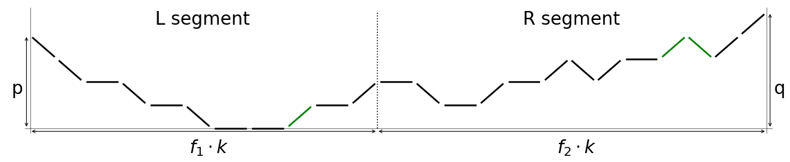
Figure 8: The initial walk $w$ (a) and the fully modified one $w^{\prime}$ (b). Only the three steps shown in green have been changed, but the enclosed area has been greatly reduced. This means that $w$ contributes less than $w^{\prime}$ to the ground state (eq. (6.23)).

The constructed mapping is not injective, as several different choices of $w$ can lead to the same resulting $w^{\prime}$. To obtain a valid relation between normalization factors, we must bound the cardinality of the preimage for an arbitrary $w^{\prime}\in H^{LR}_{p,q}$. We have established that the mapping changes at most three steps in the entire walk. So there are at most ${(f_{1}+f_{2})k\choose 3}$ choices for the locations at which changes are operated. Each change is uniquely specified, and therefore no more than ${(f_{1}+f_{2})k\choose 3}$ elements of $H^{L,1}_{p,q}$ get mapped to the same target in $H^{LR}_{p,q}$. Combining this with eq. (6.18) we find

$$N^{L,1}_{p,q} =\sum_{w\in H^{L,1}_{p,q}}t^{2A(w)}<{(f_{1}+f_{2})k\choose 3}\sum_{w^{\prime}\in H^{LR}_{p,q}}t^{2\big{(}A(w^{\prime})+(f_{2}-a_{2})k\big{)}}$$ (6.19)

$$N^{L,1}_{p,q} <\left[{(f_{1}+f_{2})k\choose 3}\cdot t^{2(f_{2}-a_{2})k}\right]\cdot\sum_{w^{\prime}\in H^{LR}_{p,q}}t^{2A(w^{\prime})}$$ (6.20)

The last sum on the RHS is precisely $AN_{p,q}$, so

$${N^{L,1}_{p,q}\over AN_{p,q}}<{(f_{1}+f_{2})k\choose 3}t^{2k(f_{2}-a_{2})}<(f_{1}+f_{2})^{3}\cdot k^{3}t^{2k(f_{2}-a_{2})}$$ (6.21)

This holds uniformly in $p<a_{1}k$ and $q<a_{2}k$, so

$$\sup\limits_{\begin{subarray}{c}p<a_{1}k\\ q<a_{2}k\end{subarray}}\left({N^{L,1}_{p,q}\over AN_{p,q}}\right)<(f_{1}+f_{2})^{3}\cdot k^{3}t^{2k(f_{2}-a_{2})}$$ (6.22)

Since $f_{2}-a_{2}>0$ and $t<1$, the RHS of the above goes to zero exponentially fast as $k\to\infty$, completing the proof of Proposition 6.10. ∎

As suggested at various points in the proof, the result generalizes to higher values of $h$:

Proposition 6.15.

For any $h\geq 1$, the ratio of $N^{L,h+1}_{p,q}$ to $N^{L,h}_{p,q}$ obeys

$$\sup\limits_{\begin{subarray}{c}p<a_{1}k\\ q<a_{2}k\end{subarray}}\left({N^{L,h+1}_{p,q}\over N^{L,h}_{p,q}}\right)<(f_{1}+f_{2})^{3}\cdot k^{3}t^{2k(f_{2}-a_{2})}$$ (6.23)

and therefore also vanishes even when multiplied by any polynomial in $k$:

$$\forall n\in\mathbb{N}:\qquad\qquad\lim\limits_{k\to\infty}\left[k^{n}\cdot\sup\limits_{\begin{subarray}{c}p<a_{1}k\\ q<a_{2}k\end{subarray}}\left({N^{L,h+1}_{p,q}\over N^{L,h}_{p,q}}\right)\right]=0$$ (6.24)

The proof of Proposition 6.15 is essentially identical to that of Proposition 6.10, so it is omitted. We will use the result to finish the proof of Lemma 6.8. The exponential term makes it straightforward to find a bound on the sum of $N^{L,h}_{p,q}$ over all $h$. At large enough $k$, the RHS of (6.23) is below 1, and so $N^{L,h+1}_{p,q}\leq N^{L,h}_{p,q}$ for all $h\geq 1$. By simple induction, it holds true that $N^{L,h}_{p,q}\leq N^{L,1}_{p,q}$. Then, recalling that $N^{L,h}_{p,q}$ vanishes for all $h>q$ and that $q<f_{2}k$, observe

$$N^{L}_{p,q}=\sum_{h=1}^{q}N^{L,h}_{p,q}\leq\sum_{h=1}^{q}N^{L,1}_{p,q}<f_{2}k\cdot N^{L,1}_{p,q}<f_{2}(f_{1}+f_{2})^{3}\cdot k^{4}t^{2k(f_{2}-a_{2})}\cdot AN_{p,q}$$ (6.25)

Similarly one can show that, for the $N^{R}_{p,q}$ factors, we obtain

$$N^{R}_{p,q}<f_{1}(f_{1}+f_{2})^{3}\cdot k^{4}t^{2k(f_{1}-a_{1})}\cdot AN_{p,q}$$ (6.26)

Since $N_{p,q}>AN_{p,q}$, it follows that

$${N^{L}_{p,q}\over N_{p,q}}<f_{2}(f_{1}+f_{2})^{3}\cdot k^{4}t^{2k(f_{2}-a_{2})}\quad\quad\text{and}\quad\quad{N^{R}_{p,q}\over N_{p,q}}<f_{1}(f_{1}+f_{2})^{3}\cdot k^{4}t^{2k(f_{1}-a_{1})}$$ (6.27)

so by adding them up, when $k$ is large enough we have that

$$1-|\langle{GS_{p,q}}|{AGS_{p,q}}\rangle|^{2}<f_{2}(f_{1}+f_{2})^{3}\cdot k^{4}t^{2k(f_{2}-a_{2})}+f_{1}(f_{1}+f_{2})^{3}\cdot k^{4}t^{2k(f_{1}-a_{1})}$$ (6.28)

holds true at all $p<a_{1}k$ and $q<a_{2}k$, which justifies the addition of the supremum:

$$\sup\limits_{\begin{subarray}{c}p<a_{1}k\\ q<a_{2}k\end{subarray}}\Big{(}1-|\langle{GS_{p,q}}|{AGS_{p,q}}\rangle|^{2}\Big{)}<f_{2}(f_{1}+f_{2})^{3}\cdot k^{4}t^{2k(f_{2}-a_{2})}+f_{1}(f_{1}+f_{2})^{3}\cdot k^{4}t^{2k(f_{1}-a_{1})}$$ (6.29)

Since both terms on the RHS of the above inequality decay exponentially fast in $k$, the desired result follows: for all $n\in\mathbb{N}$,

$$\lim\limits_{k\to\infty}\left[k^{n}\cdot\sup\limits_{\begin{subarray}{c}p<a_{1}k\\ q<a_{2}k\end{subarray}}\Big{(}1-|\langle{GS_{p,q}}|{AGS_{p,q}}\rangle|^{2}\Big{)}\right]=0$$ (6.30)

∎

We will now use the result of Lemma 6.8 to prove Lemma 6.5. For the proof, we will require a different characterization of the approximate ground state (6.8):

Proposition 6.16.

Given Assumption 6.2 and Notation 6.3, we have that, at all $p<a_{1}k$ and $q<a_{2}k$,

$$\sqrt{AN^{S}_{p,q}}\cdot|{AGS^{S}_{p,q}}\rangle=\sum_{w\in H^{LR}_{p,q}}t^{A(w)}|{w}\rangle=\sum_{r}|{UGS^{L}_{p,r}}\rangle|{UGS^{R}_{p,r}}\rangle$$ (6.31)

Proof of Proposition 6.16.

We will classify the walks by the height that they reach at the separation point between segments $L$ and $R$. Specifically, let $I_{p,q}^{r}$ be the set of walks in $H^{LR}_{p,q}$ that reach height $r$ at the separation point. It is clear from this definition that $H^{LR}_{p,q}$ is the disjoint union

$$H^{LR}_{p,q}=\bigcup_{r}I_{p,q}^{r}$$ (6.32)

where $r$ in principle runs from 0 to $\min(|L|-p,|R|-q)$. With $|L|=f_{1}k$ and $p<a_{1}k<(f_{1}-b)k$ we see that $|L|-p>bk$. Similarly, $|R|-q>bk$ and so the union over $r$ in eq. (6.32) contains more than $bk$ nonempty terms. The sum in eq. (6.31) breaks up as

$$\sum_{w\in H^{LR}_{p,q}}t^{A(w)}|{w}\rangle=\sum_{r}\sum_{w\in I^{r}_{p,q}}t^{A(w)}|{w}\rangle$$ (6.33)

Every walk in $I^{r}_{p,q}$ starts from height $p$ on the left, reaches $r$ at the separation point, and ends at $q$, while also reaching zero height within both $L$ and $R$. It can therefore be viewed as the concatenation of a walk $w_{1}$ on $L$ with imbalance $(p,r)$, and a walk $w_{2}$ on the $R$ segment with $(r,q)$ respectively.

Conversely, for any two walks $w_{1}\in G^{L}_{p,r}$ and $w_{2}\in G^{R}_{r,q}$, their concatenation (which we will denote by $w_{1}+w_{2}$) lies in $I^{r}_{p,q}$. We have therefore that the concatenation map between the Cartesian product $G^{L}_{p,r}\times G^{R}_{r,q}$ and $I^{r}_{p,q}$ is bijective. We then find

$$\sum_{w\in I^{r}_{p,q}}t^{A(w)}|{w}\rangle=\sum_{w_{1}\in G^{L}_{p,r}}\sum_{w_{2}\in G^{R}_{r,q}}t^{A(w_{1}+w_{2})}|{w_{1}+w_{2}}\rangle$$ (6.34)

Note that the state $|{w_{1}+w_{2}}\rangle$ can be written simply as $|{w_{1}}\rangle|{w_{2}}\rangle$. When concatenating walks $w_{1}$ and $w_{2}$, since they have the same height at the separation point, their enclosed areas add:

$$A(w_{1}+w_{2})=A(w_{1})+A(w_{2})$$ (6.35)

The sum in eq. (6.34) then factorizes:

$$\sum_{w_{1}\in G^{L}_{p,r}}\sum_{w_{2}\in G^{R}_{r,q}}t^{A(w_{1})+A(w_{2})}|{w_{1}}\rangle|{w_{2}}\rangle=\left(\sum_{w_{1}\in G^{L}_{p,r}}t^{A(w_{1})}|{w_{1}}\rangle\right)\left(\sum_{w_{2}\in G^{R}_{r,q}}t^{A(w_{2})}|{w_{2}}\rangle\right)$$ (6.36)

The first term is precisely $|{UGS^{L}_{p,r}}\rangle$, while the second is $|{UGS^{R}_{r,q}}\rangle$. Combining eqs. (6.33), (6.34) and (6.36) we find

$$\sum_{w\in G^{LR}_{p,q}}t^{A(w)}|{w}\rangle=\sum_{r}|{UGS^{L}_{p,r}}\rangle|{UGS^{R}_{r,q}}\rangle$$ (6.37)

completing the proof of Proposition 6.16. ∎

From considering the norms of states on either side of the equation in Prop. 6.16, we find a different characterization of $AN_{p,q}$:

$$AN_{p,q}=\sum_{r}N^{L}_{p,r}\cdot N^{R}_{r,q}$$ (6.38)

Remark.

The reason why it was imposed in the first place that $p<a_{1}k<(f_{1}-b)k$ was to allow for the existence of ground states on $L$ with $(p,r)$ unbalanced steps for all $r<bk$. The same goes for $R$ and ground states with $(r,q)$ unbalanced steps.

6.3 Proof of the section’s main result

Proof of Lemma 6.5.

Similarly to the proof of Lemma 6.8, one can write

$$\langle{AGS_{p,q}}|{ATGS_{p,q}}\rangle={\sum_{r<bk}\langle{UGS^{L}_{p,r}}|{UGS^{L}_{p,r}}\rangle\langle{UGS^{R}_{r,q}}|{UGS^{R}_{r,q}}\rangle\over\sqrt{ATN_{p,q}\cdot AN_{p,q}}}={\sum_{r<bk}N^{L}_{p,r}N^{R}_{r,q}\over\sqrt{ATN_{p,q}\cdot AN_{p,q}}}=\sqrt{ATN_{p,q}\over AN_{p,q}}$$ (6.39)

and the sums in the normalization factors can be split by defining

$$N^{r}_{p,q}=N^{L}_{p,r}\cdot N^{R}_{r,q}\quad\implies\quad AN_{p,q}=\sum_{r}N^{r}_{p,q}\quad\quad\text{and}\quad\quad ATN_{p,q}=\sum_{r<bk}N^{r}_{p,q}$$ (6.40)

We can relate $N^{r+1}_{p,q}$ to $N^{r}_{p,q}$ through a lowering procedure as before. Take a walk $w$ that has $(p,q)$ unbalanced steps on the full chain, and also has height $r+1$ at the border between the two segments. We have seen that $w$ can be viewed as a concatenation of $w_{1}\in G^{L}_{p,r+1}$, and $w_{2}\in G^{R}_{r+1,q}$.

Consider the leftmost unbalanced up step of $w_{1}$ and the rightmost unbalanced down one of $w_{2}$. It follows from Proposition 6.11 that the portion of $w$ between them is located at heights 1 or higher, so these two steps are balancing partners within $w$ (Fig. 9a). Replace both of them by flat steps (Fig. 9b). This has the effect of lowering the ‘central peak’ by one unit, while leaving the rest of the walk unchanged. Therefore it maps the walk $w$ to one with the same overall number $(p,q)$ of unbalanced steps, but with a lower central peak. Namely, the resulting walk $w^{\prime}$ is a concatenation of $w_{1}^{\prime}\in G^{L}_{p,r}$, and $w_{2}^{\prime}\in G^{R}_{r,q}$. The area under $w^{\prime}$ is reduced by at least $2r-1$ units, compared to that under $w$.

Figure 9: The initial walk (a) and the modified one (b). The unbalanced up-steps on $L$ and down-steps on $R$, which contribute to the central peak, are shown in orange (all but the furthermost ones) or red (the extremal ones, which get flattened in the transformation). Only two steps are changed, but the area under the central peak is greatly reduced. Consequently, the (a) walk is suppressed more than (b) within a ground state (eq. (6.41)).

Same as before, the mapping is not injective and we can bound the cardinality of the preimage for any target point by ${(f_{1}+f_{2})k\choose 2}$, which translates into the ratio of successive normalization factors being bounded as follows:

$${N^{r+1}_{p,q}\over N^{r}_{p,q}}<t^{2(2r-1)}{(f_{1}+f_{2})k\choose 2}$$ (6.41)

If $r\geq bk$, then the exponent grows linearly with $k$. The combinatorial factor can be bounded above by $(f_{1}+f_{2})^{2}k^{2}$, and then one can sum over $r$ (where we have at most $(f_{1}+f_{2})k$ terms, since no walk can possibly reach greater heights than that, being limited by the system size) to find

$$\sup\limits_{\begin{subarray}{c}p<a_{1}k\\ q<a_{2}k\end{subarray}}\Big{(}1-|\langle{AGS_{p,q}}|{ATGS_{p,q}}\rangle|^{2}\Big{)}<(f_{1}+f_{2})^{3}k^{3}\cdot t^{4bk-2}$$ (6.42)

Due to the exponential factor, then, we have

$$\forall n\in\mathbb{N}:\qquad\qquad\lim\limits_{k\to\infty}\left[k^{n}\cdot\sup\limits_{\begin{subarray}{c}p<a_{1}k\\ q<a_{2}k\end{subarray}}\Big{(}1-|\langle{AGS_{p,q}}|{ATGS_{p,q}}\rangle|^{2}\Big{)}\right]=0$$ (6.43)

and combining this with the results of Lemmas 6.8 and B.2, it follows that

$$\forall n\in\mathbb{N}:\qquad\qquad\lim\limits_{k\to\infty}\left[k^{n}\cdot\sup\limits_{\begin{subarray}{c}p<a_{1}k\\ q<a_{2}k\end{subarray}}\Big{(}1-|\langle{GS_{p,q}}|{ATGS_{p,q}}\rangle|^{2}\Big{)}\right]=0$$ (6.44)

completing the proof. ∎

7 High-imbalance approximations

Having covered the regime of low-$p$ and low-$q$, it remains to find a complementary approximation lemma, which applies when either the high-$p$ or the high-$q$ regime is present. This situation is simpler, since the ground state will be dominated by walks whose unbalanced steps are pushed outwards, and so it approximately factorizes. The setup is the following:

Assumption 7.1.

Let $f_{1}$, $f_{2}>0$ be given constants, and fix some small $c$ with $0<c<1/4-2b$.

Notation 6.3 remains in the same form.

Definition 7.2.

For every segment in Notation 6.3 we define an approximate ground state with $(p,q)$ unbalanced steps, which will be useful in the high-$q$ regime, as

$$|{PGS^{(R)}_{p,q}}\rangle=|{GS^{L}_{p,q-f_{2}k}}\rangle\otimes\big{(}|{u}\rangle\big{)}^{\otimes f_{2}k}$$ (7.1)

where the $k$ label was suppressed for simplicity in the naming of all states, and the $|{GS}\rangle$ state is in accordance with Definition 4.5. The main property of this state is that it contains exclusively up steps in the $R$ segment. The analogous state which is useful in the high-$p$ regime is

$$|{PGS^{(L)}_{p,q}}\rangle=\big{(}|{d}\rangle\big{)}^{\otimes f_{1}k}\otimes|{GS^{R}_{p-f_{1}k,q}}\rangle$$ (7.2)

with exclusively down steps in the $L$ segment.

The result of this section is:

Lemma 7.3.

Given Assumption 7.1 and Notation 6.3, and with Definitions 6.1 and 7.2, the product state in (7.1) superpolynomially approximates the true ground state when $q>(f_{2}+c)k$:

$$\forall n\in\mathbb{N}:\qquad\qquad\lim\limits_{k\to\infty}\left[k^{n}\cdot\sup\limits_{q>(f_{2}+c)k}\Big{(}1-|\langle{GS_{p,q}}|{PGS^{(R)}_{p,q}}\rangle|^{2}\Big{)}\right]=0$$ (7.3)

and similarly the state in (7.2) is a good approximation when $p>(f_{1}+c)k$:

$$\forall n\in\mathbb{N}:\qquad\qquad\lim\limits_{k\to\infty}\left[k^{n}\cdot\sup\limits_{p>(f_{1}+c)k}\Big{(}1-|\langle{GS_{p,q}}|{PGS^{(L)}_{p,q}}\rangle|^{2}\Big{)}\right]=0$$ (7.4)

We begin with a preliminary discussion, and then proceed to prove the lemma. In what follows we will only discuss the high$-q$ case and prove eq. (7.3), as the argument for (7.4) in the high-$p$ regime will be identical.

7.1 Splitting the ground states

For any walk $w$ in the high-$q$ regime, all heights reached within the $R$ segment are relatively large (i.e. are bounded below by $ck$). Placing a flat or down step in this segment (as opposed to an up one) will carry a significant additional area cost. For this reason, we expect walks that do not exclusively contain up steps within $R$ to be exponentially suppressed. To make this precise, work with Notation 6.3. We classify walks by the number of balanced steps they contain in the $R$ segment:

Definition 7.4.

Let $G^{S;\;z}_{p,q}$ be the collection of walks in $G^{S}_{p,q}$ that contain exactly $z$ balanced steps in the $R$ segment (see Figure 10). Throughout the rest of the section, we will only take the segment $S$ as in Notation 6.3, and we omit the corresponding $S$ label, to simplify the notation as $G^{z}_{p,q}\subset G_{p,q}$. Also let $N^{z}_{p,q}$ be the contribution to normalization due to walks in $G^{z}_{p,q}$ only:

$$N^{z}_{p,q}\equiv\sum_{w\in G^{z}_{p,q}}t^{2A(w)}$$ (7.5)

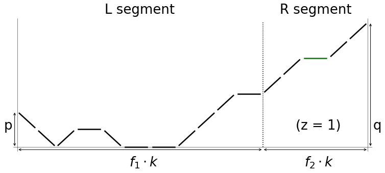
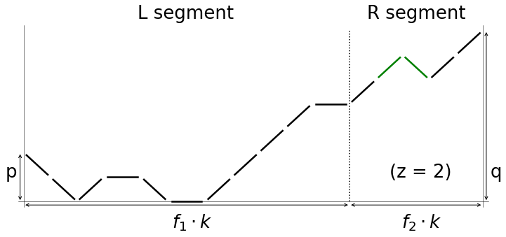
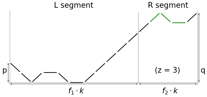
Figure 10: Typical walks in $G^{z}_{p,q}$ for $z$ equal to 0, 1, 2, and 3. The balanced steps contributing to the count of $z$ are shown in green. As $z$ increases, the total area under typical walks becomes larger, and so their contribution within a ground state is exponentially suppressed (eq. (7.15)).

From this definition it follows that $G_{p,q}$ is the disjoint union over $z$ of the $G^{z}_{p,q}$. The unnormalized, exact ground state is as in Definition 4.5:

$$|{UGS_{p,q}}\rangle=\sum_{w\in G_{p,q}}t^{A(w)}|{w}\rangle=\sum_{z}\sum_{w\in G^{z}_{p,q}}t^{A(w)}|{w}\rangle$$ (7.6)

where the $z$ index in the summation goes from zero up to, nominally, $f_{2}k$ (i.e. when all steps in the $R$ segment are balanced). Note that the subcollections $G^{z}_{p,q}$ with $z$ close to this upper limit of $f_{2}k$ will often be empty due to constraints imposed by the total length of the spin chain; however this will not matter further in the argument.

To normalize the state in (7.6), find $N_{p,q}=\langle{UGS_{p,q}}|{UGS_{p,q}}\rangle$. The $G^{z}_{p,q}$ with different $z$ are disjoint, so

$$N_{p,q}=\sum_{z}\sum_{w\in G^{z}_{p,q}}t^{2A(w)}=\sum_{z}N^{z}_{p,q}$$ (7.7)

such that the exact ground state is

$$|{GS_{p,q}}\rangle={1\over\sqrt{N_{p,q}}}\sum_{z}\sum_{w\in G^{z}_{p,q}}t^{A(w)}|{w}\rangle$$ (7.8)

The claim is that, at large enough $q$, the $N^{0}_{p,q}$ term dominates all others in the sum for $N_{p,q}$ (eq. (7.7)). That enables us to approximate the true ground state (7.8) by the $z=0$ component only:

$$|{GS^{(z=0)}_{p,q}}\rangle\equiv{1\over\sqrt{N^{0}_{p,q}}}\sum_{w\in G^{0}_{p,q}}t^{A(w)}|{w}\rangle$$ (7.9)

Proposition 7.5.

The $|{GS^{(z=0)}_{p,q}}\rangle$ defined above is identical to the $|{PGS^{(R)}_{p,q}}\rangle$ of eq. (7.1).

Proof of Proposition 7.5.

The condition of having $z=0$ balanced steps in the $R$ segment means that all walks in $G^{0}_{p,q}$ have their last $f_{2}k$ steps all up. We are placing no restriction on the steps in the $L$ segment, and since we’re taking the area-weighted superposition of all possible walks, we see that we form exactly the ground state on the $L$ segment, with the corresponding numbers $(p,q-f_{2}k)$ of unbalanced steps:

$${1\over\sqrt{N^{0}_{p,q}}}\sum_{w\in G^{0}_{p,q}}t^{A(w)}|{w}\rangle=|{GS^{L}_{p,q-f_{2}k}}\rangle\otimes\big{(}|{u}\rangle\big{)}^{\otimes f_{2}k}\equiv|{PGS^{(R)}_{p,q}}\rangle$$ (7.10)

∎

The characterization (7.10) shows that $|{PGS^{(R)}_{p,q}}\rangle$ consists precisely of the walks in $G^{0}_{p,q}$, with the correct area weights. This additional result will help us to prove Lemma 7.3.

7.2 Proof of the section’s main result

Proof of Lemma 7.3.

The proof is very similar to that of Lemma 6.8. From equations (7.8) and (7.10), we find

$$\langle{GS_{p,q}}|{PGS^{R}_{p,q}}\rangle={1\over\sqrt{N_{p,q}\cdot N^{0}_{p,q}}}\sum_{w\in G^{0}_{p,q}}t^{2A(w)}={N^{0}_{p,q}\over\sqrt{N_{p,q}\cdot N^{0}_{p,q}}}\quad\implies\quad|\langle{GS_{p,q}}|{PGS^{R}_{p,q}}\rangle|^{2}={N^{0}_{p,q}\over N_{p,q}}$$ (7.11)

which combined with eq. (7.7) gives

$$|\langle{GS_{p,q}}|{PGS^{R}_{p,q}}\rangle|^{2}=1-\sum_{z>0}{N^{z}_{p,q}\over N_{p,q}}\quad\implies\quad 1-|\langle{GS_{p,q}}|{PGS^{R}_{p,q}}\rangle|^{2}=\sum_{z>0}{N^{z}_{p,q}\over N_{p,q}}$$ (7.12)

As before, the strategy is to map walks in $G^{z}_{p,q}$ to walks in $G^{z-1}_{p,q}$ and obtain an upper bound on $N^{z}_{p,q}/N^{z-1}_{p,q}$. For any $z>0$, take any $w\in G^{z}_{p,q}$, and let $b_{1}$ be its rightmost balanced step. Since $z>0$, the $R$ segment contains a positive number of balanced steps, and in particular $b_{1}$ must be in $R$ (Fig. 11a).

The step $b_{1}$ must be flat or down, because any balanced up-step has a partner to its right. The following steps of the proof will require $b_{1}$ to be flat. If instead it is down, find its balancing partner and replace them both by flat steps. (This procedure only lowers the area; Fig. 11b). Note that the two flat steps we’ve introduced are still balanced, so this leaves the walk in $G^{z}_{p,q}$.

Next, find the first unbalanced up-step $s_{1}$. Since there are at least $(f_{2}+c)k$ of them (from the condition on $q$), we see that $s_{1}$ must be at least $(f_{2}+c)k$ positions away from the rightmost end of the chain, i.e. at least $ck$ positions to the left of the boundary between $L$ and $R$. As $b_{1}$ is in $R$, we obtain that the distance between the two is at least $ck$:

$$d(s_{1},b_{1})>ck$$ (7.13)

Interchanging $s_{1}$ and $b_{1}$ to form a walk $w^{\prime}$ then lowers the area by at least $ck$ units (Fig. 11c). This swap eliminated a balanced step from the rightmost segment, so $w^{\prime}\in G^{z-1}_{p,q}$ (Fig. 11d).

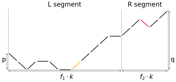
Figure 11: Typical walk in $G^{2}_{p,q}$, and an illustration of the swap procedure. In (a), the leftmost unbalanced step $s_{1}$ is orange and the rightmost balanced one $b_{1}$ is red. Since $b_{1}$ is down, it needs to be flattened; this is shown in (b), with the former balancing partner shown in green. In (c), $s_{1}$ and $b_{1}$ are exchanged, and the purple section shifts down by one unit as a result. In the end, only three steps have been altered, shown in green in (d). The final result belongs to $G^{1}_{p,q}$, and encloses a smaller area, helping to prove eq. (7.15).

Similarly to the previous section, the mapping is not injective, and we need to bound the cardinality of the preimage for any given $w^{\prime}\in G^{z-1}_{p,q}$. The treatment of this aspect is identical to that in the proof of Lemma 6.8, with the result that the desired cardinality is at most ${(f_{1}+f_{2})k\choose 3}$. Combining this with eq. (7.13), we obtain

$$N^{z+1}_{p,q}=\sum_{w\in G^{z+1}_{p,q}}t^{2A(w)}<{(f_{1}+f_{2})k\choose 3}\sum_{w\in G^{z}_{p,q}}t^{2\big{(}A(w)+ck\big{)}}$$ (7.14)

and so

$${N^{z+1}_{p,q}\over N^{z}_{p,q}}<{(f_{1}+f_{2})k\choose 3}t^{2kc}<(f_{1}+f_{2})^{3}\cdot k^{3}t^{2kc}.$$ (7.15)

Since $c>0$ and $t<1$, the RHS of the above goes to zero exponentially fast as $k\to\infty$. At large enough $k$ this implies monotonicity in $z$, $N^{z+1}_{p,q}<N^{z}_{p,q}$, and so in particular we can use $N^{z}_{p,q}<N^{1}_{p,q}$ to bound the sum over $z$ in the RHS of eq. (7.12) as

$$\sum_{z=1}^{f_{2}k}{N^{z}_{p,q}\over N^{0}_{p,q}}<\sum_{z=1}^{f_{2}k}{N^{1}_{p,q}\over N^{0}_{p,q}}=f_{2}k\cdot{N^{1}_{p,q}\over N^{0}_{p,q}}<f_{2}(f_{1}+f_{2})^{3}\cdot k^{4}t^{2kc}$$ (7.16)

By construction $N^{0}_{p,q}<N_{p,q}$, so replacing the denominator $N^{0}_{p,q}$ by $N_{p,q}$ in the sum above will only make it smaller:

$$\sum_{z>0}{N^{z}_{p,q}\over N_{p,q}}<\sum_{z>0}{N^{z}_{p,q}\over N^{0}_{p,q}}<f_{2}(f_{1}+f_{2})^{3}\cdot k^{4}t^{2kc}$$ (7.17)

and it follows that

$$1-|\langle{GS_{p,q}}|{PGS^{R}_{p,q}}\rangle|^{2}=\sum_{z>0}{N^{z}_{p,q}\over N_{p,q}}<f_{2}(f_{1}+f_{2})^{3}\cdot k^{4}t^{2kc}$$ (7.18)

The above is valid for all $q>(f_{2}+c)k$, but the RHS does not involve $q$. We take the supremum of the LHS over $q$ in this range:

$$\sup\limits_{q>(f_{2}+c)k}\Big{(}1-|\langle{GS_{p,q}}|{PGS^{R}_{p,q}}\rangle|^{2}\Big{)}<f_{2}(f_{1}+f_{2})^{3}\cdot k^{4}t^{2kc}$$ (7.19)

Due to the exponential factor on the right, eq. (7.3) follows. As mentioned previously, an identical argument shows that eq. (7.4) is also true, completing the proof of the lemma. ∎

8 Implementing the approximations

8.1 Imbalance regimes and splitting the chain

We now use the approximations of sections 6 and 7 to find the limiting behavior in $k$ of the quantity

$$\sup\limits_{\begin{subarray}{c}p,q\geq 0\\ p+q\leq 3k\end{subarray}}\left(\sup\limits_{\phi_{p,q}\in\operatorname{range}E_{k}}\langle{\phi_{p,q}}|{G_{[k+1,3k]}}|{\phi_{p,q}}\rangle\right)$$ (8.1)

which appears in the RHS of Proposition 4.9. Fix a constant $c\in(0,1/4-2b)$, which one may imagine to be very small. We will cover the following distinct regimes:

• $p>k\left(1+{c\over 2}\right)$, $q$ arbitrary, but still consistent with $p$, i.e. $q+p\leq 3k$

• $q>k\left(1+{c\over 2}\right)$, $p$ arbitrary (but still consistent with $q$)

• $p,q<k\left(1+c\right)$

The three cases are not mutually exclusive, but their union covers all possible values for $p$ and $q$ on a chain segment of length $3k$. For large numbers of unbalanced steps, we directly show that

Proposition 8.1.

For the large-$p$ regime, $p>k\left(1+{c\over 2}\right)$, we have

$$\lim\limits_{k\to\infty}\left(\sup\limits_{\begin{subarray}{c}(1+c/2)k<p\leq 3k\\ 0\leq q\leq 3k-p\end{subarray}}\left(\sup\limits_{|{\phi_{p,q}}\rangle\in\operatorname{range}E_{k}}\langle{\phi_{p,q}}|{G_{[k+1,3k]}}|{\phi_{p,q}}\rangle\right)\right)=0$$ (8.2)

and similarly in the regime where $q$ is larger than $k\left(1+{c\over 2}\right)$:

$$\lim\limits_{k\to\infty}\left(\sup\limits_{\begin{subarray}{c}(1+c/2)k<q\leq 3k\\ 0\leq p\leq 3k-q\end{subarray}}\left(\sup\limits_{|{\phi_{p,q}}\rangle\in\operatorname{range}E_{k}}\langle{\phi_{p,q}}|{G_{[k+1,3k]}}|{\phi_{p,q}}\rangle\right)\right)=0$$ (8.3)

For the low-imbalance regime, we find a similar result, albeit through a longer argument:

Proposition 8.2.

In the $p,q<(1+c)\cdot k$ regime it is true that

$$\lim\limits_{k\to\infty}\left(\sup\limits_{0\leq p,q<(1+c)k}\left(\sup\limits_{|{\phi_{p,q}}\rangle\in\operatorname{range}E_{k}}\langle{\phi_{p,q}}|{G_{[k+1,3k]}}|{\phi_{p,q}}\rangle\right)\right)=0$$ (8.4)

We then combine Propositions 8.1 and 8.2 to conclude that the supremum over all possible $p,q$ goes to zero in the limit of large $k$:

Proposition 8.3.

From Propositions 8.1 and 8.2 it follows that

$$\lim\limits_{k\to\infty}\left(\sup\limits_{\begin{subarray}{c}p,q\geq 0\\ p+q\leq 3k\end{subarray}}\left(\sup\limits_{|{\phi_{p,q}}\rangle\in\operatorname{range}E_{k}}\langle{\phi_{p,q}}|{G_{[k+1,3k]}}|{\phi_{p,q}}\rangle\right)\right)=0$$ (8.5)

Proof of Proposition 8.3.

As discussed in the beginning of this section, the ranges of $p,q$ covered in Propositions 8.1 and 8.2 can be combined to cover all the possibilities for $p,q\geq 0$ with $p+q\leq 3k$. ∎

We now turn to proving Propositions 8.1 and 8.2. The former is a direct application of the results in Section 7. The latter proof relies on Section 6 in a similar manner, but also requires more in-depth technical discussions, which are presented separately in Section 9 and appendix A.

8.2 High imbalance

Since ground states with a large number of unbalanced steps approximately factorize, verification of the criterion is more straightforward in this case.

Proof of Proposition 8.1.

We will work in the large $p$ regime, and show that eq. (8.2) holds. By assumption, $|{\phi_{p,q}}\rangle$ is orthogonal to the ground space on the full chain:

$$G_{[1,3k]}|{\phi_{p,q}}\rangle=0$$ (8.6)

Expanding $G_{[1,3k]}$ in terms of individual ground states, we note that only the state with $(p,q)$ unbalanced steps can contribute. Therefore, the above translates to

$$\langle{GS_{p,q}^{[1,3k]}}|{\phi_{p,q}}\rangle=0\qquad\implies\qquad\langle{\phi_{p,q}}|{GS_{p,q}^{[1,3k]}}\rangle\langle{GS_{p,q}^{[1,3k]}}|{\phi_{p,q}}\rangle=0$$ (8.7)

With $p>(1+c)k$, we can use the high imbalance approximation Lemma 7.3, with $L=[1,k]$ and $R=[k+1,3k]$ to approximate $|{GS_{p,q}^{[1,3k]}}\rangle$ by

$$|{PGS_{p,q}^{[1,3k]}}\rangle=|{d}\rangle^{\otimes k}\otimes|{GS_{p-k,q}^{[k+1,3k]}}\rangle$$ (8.8)

and it follows by the projector approximation Lemma B.16 that the quantities $|\langle{PGS_{p,q}^{[1,3k]}}|{\phi_{p,q}}\rangle|^{2}$ approximate $|\langle{GS_{p,q}^{[1,3k]}}|{\phi_{p,q}}\rangle|^{2}$ at large $k$. Since the latter overlaps are, by assumption, identically zero when $|{\phi_{p,q}}\rangle\in\operatorname{range}E_{k}$, we find

$$\lim\limits_{k\to\infty}\left(\sup\limits_{\begin{subarray}{c}(1+c/2)k<p\leq 3k\\ 0\leq q\leq 3k-p\end{subarray}}\left(\sup\limits_{|{\phi_{p,q}}\rangle\in\operatorname{range}E_{k}}\langle{\phi_{p,q}}|{PGS_{p,q}^{[1,3k]}}\rangle\langle{PGS_{p,q}^{[1,3k]}}|{\phi_{p,q}}\rangle\right)\right)=0$$ (8.9)

The projector onto $PGS$ can be decomposed as a tensor product:

$$|{PGS_{p,q}^{[1,3k]}}\rangle\langle{PGS_{p,q}^{[1,3k]}}|=|{d}\rangle^{\otimes k}\langle{d}|^{\otimes k}\otimes|{GS_{p-k,q}^{[k+1,3k]}}\rangle\langle{GS_{p-k,q}^{[k+1,3k]}}|$$ (8.10)

Note that when this acts on $|{\phi_{p,q}}\rangle$, the second component behaves like $G_{[k+1,3k]}$. The reason is that $|{d}\rangle^{\otimes k}\langle{d}|^{\otimes k}$ selects only walks with the first $k$ steps down. Since every walk of $|{\phi_{p,q}}\rangle$ has $(p,q)$ unbalanced steps on $[1,3k]$, those with the first $k$ steps down will have $(p-k,q)$ unbalanced steps on $[k+1,3k]$. Therefore, the only ground state they need to be compared to is $|{GS_{p-k,q}^{[k+1,3k]}}\rangle$. This allows for the rewriting of (8.9) as

$$\lim\limits_{k\to\infty}\left(\sup\limits_{\begin{subarray}{c}(1+c/2)k<p\leq 3k\\ 0\leq q\leq 3k-p\end{subarray}}\left(\sup\limits_{|{\phi_{p,q}}\rangle\in\operatorname{range}E_{k}}\langle{\phi_{p,q}}|\Big{(}|{d}\rangle^{\otimes k}\langle{d}|^{\otimes k}\otimes G_{[k+1,3k]}\Big{)}|{\phi_{p,q}}\rangle\right)\right)=0$$ (8.11)

This form is close to the desired result, but has the extra $|{d}\rangle^{\otimes k}\langle{d}|^{\otimes k}$ projector. Some walks in the composition of $|{\phi_{p,q}}\rangle$ will have their first $k$ steps down, and others will not. Equation (8.11) deals with those that do, and one must separately consider the ones that do not. This will be addressed as follows: since $|{\phi_{p,q}}\rangle$ is in the range of $E_{k}$, it consists only of ground states on the first two thirds of the chain $[1,2k]$. Namely, it is an eigenstate of the projector $G_{[1,2k]}$, with eigenvalue 1:

$$|{\phi_{p,q}}\rangle=G_{[1,2k]}|{\phi_{p,q}}\rangle$$ (8.12)

This allows for a Schmidt decomposition of $|{\phi_{p,q}}\rangle$ with respect to subsystems $[1,2k]$ and $[2k+1,3k]$, in which only ground states will be present on the left side. To determine which numbers of unbalanced steps can appear in this decomposition, we must carefully analyze the minimization of walks. Recall that a walk on $[1,3k]$ with $(p,q)$ unbalanced steps must start at height $p$, end at height $q$, and reach zero somewhere in between. Since we are assuming $p>(1+c)k$, all the points where the walk reaches zero height must be at least $(1+c)k$ steps away from the start, so in particular none of them can be found in the first third $[1,k]$. We distinguish three cases:

• Walks that reach zero height both within the middle third $[k+1,2k]$, and within the last one $[2k+1,3k]$. When we ‘cut’ them after $2k$ steps, both resulting components will still reach zero height, so they will already be minimized. If the height after $2k$ steps (at the split point) is $v$, then the resulting walks will have $(p,v)$ and $(v,q)$ unbalanced steps respectively.

• Walks that do not reach zero height in the middle third, but rather only within the last one. When splitting, the first component will not be minimized. If $z$ is the minimum height that the original walk reached within the first two thirds $[1,2k]$, and $z+v$ is the height at the split point (with $v\geq 0$), then the resulting walks have $(p-z,v)$ and $(v+z,q)$ unbalanced steps respectively.

• Walks that only reach zero height within the middle third, and not the last one. With $z$ the minimum height within the last third $[2k+1,3k]$, and $z+v$ the height at the splitting point, we find $(p,v+z)$ and $(v,q-z)$ unbalanced steps.

The resulting decomposition will be

$$|{\phi_{p,q}}\rangle=\sum_{v\geq 0}|{GS_{p,v}^{[1,2k]}}\rangle\otimes|{\psi^{1}_{v,q}}\rangle+\sum_{z=1}^{p}\sum_{v\geq 0}|{GS_{p-z,v}^{[1,2k]}}\rangle\otimes|{\psi^{2}_{v+z,q}}\rangle+\sum_{z=1}^{q}\sum_{v\geq 0}|{GS_{p,v+z}^{[1,2k]}}\rangle\otimes|{\psi^{3}_{v,q-z}}\rangle$$ (8.13)

The $\psi^{1},\psi^{2},\psi^{3}$ states all live on the last third $[2k+1,3k]$. By convention we absorb the coefficients from the Schmidt decomposition into their definition, so they are not normalized. This will not pose a problem, since the main focus will be on the properties of the $[1,2k]$ ground states instead. For simplicity of notation, give separate names to the three terms:

$$|{\mathrm{I}}\rangle =\sum_{v\geq 0}|{GS_{p,v}^{[1,2k]}}\rangle\otimes|{\psi^{1}_{v,q}}\rangle$$

$$|{\mathrm{II}}\rangle =\sum_{z=1}^{p}\sum_{v\geq 0}|{GS_{p-z,v}^{[1,2k]}}\rangle\otimes|{\psi^{2}_{v+z,q}}\rangle$$

$$|{\mathrm{III}}\rangle =\sum_{z=1}^{q}\sum_{v\geq 0}|{GS_{p,v+z}^{[1,2k]}}\rangle\otimes|{\psi^{3}_{v,q-z}}\rangle$$

The ground states that appear in $|{\mathrm{I}}\rangle$ and $|{\mathrm{III}}\rangle$ have $p$ unbalanced steps on the left, so we can use the high imbalance approximation lemma with $L=[1,k]$ and $R=[k+1,2k]$ to argue that:

• $|{GS_{p,v}^{[1,2k]}}\rangle$ is superpolynomially approximated by $|{d}\rangle^{\otimes k}\otimes|{GS_{p-k,v}^{[k+1,2k]}}\rangle$.

• $|{GS_{p,v+z}^{[1,2k]}}\rangle$ is superpolynomially approximated by $|{d}\rangle^{\otimes k}\otimes|{GS_{p-k,v+z}^{[k+1,2k]}}\rangle$.

Through an argument similar to that of the superposition approximation Lemma B.6, we conclude that $|{\mathrm{I}}\rangle$ is approximated superpolynomially by

$$|{\mathrm{I}^{\prime}}\rangle=\sum_{v\geq 0}|{d}\rangle^{\otimes k}\otimes|{GS_{p-k,v}^{[k+1,2k]}}\rangle\otimes|{\psi^{1}_{v,q}}\rangle=|{d}\rangle^{\otimes k}\otimes\left(\sum_{v\geq 0}|{GS_{p-k,v}^{[k+1,2k]}}\rangle\otimes|{\psi^{1}_{v,q}}\rangle\right)$$ (8.14)

and similarly, $|{\mathrm{III}}\rangle$ is approximated by

$$|{\mathrm{III}^{\prime}}\rangle=\sum_{z=1}^{q}\sum_{v\geq 0}|{d}\rangle^{\otimes k}\otimes|{GS_{p-k,v+z}^{[k+1,2k]}}\rangle\otimes|{\psi^{3}_{v,q-z}}\rangle=|{d}\rangle^{\otimes k}\otimes\left(\sum_{z=1}^{q}\sum_{v\geq 0}|{GS_{p-k,v+z}^{[k+1,2k]}}\rangle\otimes|{\psi^{3}_{v,q-z}}\rangle\right)$$ (8.15)

The same reasoning doesn’t directly work for $|{\mathrm{II}}\rangle$, since the ground states appearing within it only have $p-z$ unbalanced steps on the left, which is not guaranteed to be above $(1+c)k$ if $z$ is large. Instead, we will separate $|{\mathrm{II}}\rangle$ into two terms, one including the walks with the first $k$ steps down, call it $|{\mathrm{IIa}}\rangle$, and everything else, which will be called $|{\mathrm{IIb}}\rangle$. Formally,

$$|{\mathrm{II}}\rangle\equiv|{\mathrm{IIa}}\rangle+|{\mathrm{IIb}}\rangle\qquad\qquad\Big{(}|{d}\rangle^{\otimes k}\langle{d}|^{\otimes k}\Big{)}|{\mathrm{IIa}}\rangle=|{\mathrm{IIa}}\rangle\qquad\qquad\Big{(}|{d}\rangle^{\otimes k}\langle{d}|^{\otimes k}\Big{)}|{\mathrm{IIb}}\rangle=0$$ (8.16)

With $|{\phi_{p,q}}\rangle=|{\mathrm{I}}\rangle+|{\mathrm{IIa}}\rangle+|{\mathrm{IIb}}\rangle+|{\mathrm{III}}\rangle$, we define the approximation

$$|{\phi_{p,q}^{\prime}}\rangle=|{\mathrm{I}^{\prime}}\rangle+|{\mathrm{IIa}}\rangle+|{\mathrm{IIb}}\rangle+|{\mathrm{III}^{\prime}}\rangle$$ (8.17)

This is superpolynomial since $|{\mathrm{I}^{\prime}}\rangle$ and $|{\mathrm{III}^{\prime}}\rangle$ are. We will show that, at large $k$, the projector $G_{[k+1,3k]}$ approximately annihilates this. The argument is in two parts:

Proposition 8.4.

$$\lim\limits_{k\to\infty}\left(\sup\limits_{\begin{subarray}{c}(1+c/2)k<p\leq 3k\\ 0\leq q\leq 3k-p\end{subarray}}\left(\sup\limits_{|{\phi_{p,q}}\rangle\in\operatorname{range}E_{k}}\|G_{[k+1,3k]}\Big{(}|{\mathrm{I}^{\prime}}\rangle+|{\mathrm{IIa}}\rangle+|{\mathrm{III}^{\prime}}\rangle\Big{)}\|\right)\right)=0$$

Proposition 8.5.

$$\lim\limits_{k\to\infty}\left(\sup\limits_{\begin{subarray}{c}(1+c/2)k<p\leq 3k\\ 0\leq q\leq 3k-p\end{subarray}}\left(\sup\limits_{|{\phi_{p,q}}\rangle\in\operatorname{range}E_{k}}\|G_{[k+1,3k]}|{\mathrm{IIb}}\rangle\|\right)\right)=0$$

Assume these two propositions. From the triangle inequality we obtain

$$\|G_{[k+1,3k]}|{\phi_{p,q}^{\prime}}\rangle\| \leq\|G_{[k+1,3k]}\Big{(}|{\mathrm{I}^{\prime}}\rangle+|{\mathrm{IIa}}\rangle+|{\mathrm{III}^{\prime}}\rangle\Big{)}\|+\|G_{[k+1,3k]}|{\mathrm{IIb}}\rangle\|$$ (8.18)

Both terms on the last line vanish at large $k$, and so $G_{[k+1,3k]}$ approximately annihilates $|{\phi_{p,q}^{\prime}}\rangle$:

$$\lim\limits_{k\to\infty}\left(\sup\limits_{\begin{subarray}{c}(1+c/2)k<p\leq 3k\\ 0\leq q\leq 3k-p\end{subarray}}\left(\sup\limits_{|{\phi_{p,q}}\rangle\in\operatorname{range}E_{k}}\langle{\phi_{p,q}^{\prime}}|{G_{[k+1,3k]}}|{\phi_{p,q}^{\prime}}\rangle\right)\right)=0$$ (8.19)

Using the expectation approximation Lemma B.12, we conclude

$$\lim\limits_{k\to\infty}\left(\sup\limits_{\begin{subarray}{c}(1+c/2)k<p\leq 3k\\ 0\leq q\leq 3k-p\end{subarray}}\left(\sup\limits_{|{\phi_{p,q}}\rangle\in\operatorname{range}E_{k}}\langle{\phi_{p,q}}|{G_{[k+1,3k]}}|{\phi_{p,q}}\rangle\right)\right)=0$$ (8.20)

completing the proof of eq. (8.2). ∎

The argument for eq. (8.3) is very similar, so most of its details will be omitted. An outline is sketched in B.7. We turn to the proof of Proposition 8.4:

Proof of Proposition 8.4.

All terms in $|{\phi_{p,q}^{\prime}}\rangle$, except for $|{\mathrm{IIb}}\rangle$, have their first $k$ steps down, so

$$\Big{(}|{d}\rangle^{\otimes k}\langle{d}|^{\otimes k}\Big{)}\Big{(}|{\mathrm{I}^{\prime}}\rangle+|{\mathrm{IIa}}\rangle+|{\mathrm{III}^{\prime}}\rangle\Big{)}=|{\mathrm{I}^{\prime}}\rangle+|{\mathrm{IIa}}\rangle+|{\mathrm{III}^{\prime}}\rangle$$ (8.21)

and if we add a $G_{[k+1,3k]}$ projector, it follows that

$$\Big{(}|{d}\rangle^{\otimes k}\langle{d}|^{\otimes k}\otimes G_{[k+1,3k]}\Big{)}\Big{(}|{\mathrm{I}^{\prime}}\rangle+|{\mathrm{IIa}}\rangle+|{\mathrm{III}^{\prime}}\rangle\Big{)}=G_{[k+1,3k]}\Big{(}|{\mathrm{I}^{\prime}}\rangle+|{\mathrm{IIa}}\rangle+|{\mathrm{III}^{\prime}}\rangle\Big{)}$$ (8.22)

On the other hand, since $|{d}\rangle^{\otimes k}\langle{d}|^{\otimes k}$ annihilates $|{\mathrm{IIb}}\rangle$, the LHS of the above is equal to:

$$\Big{(}|{d}\rangle^{\otimes k}\langle{d}|^{\otimes k}\otimes G_{[k+1,3k]}\Big{)}\Big{(}|{\mathrm{I}^{\prime}}\rangle+|{\mathrm{IIa}}\rangle+|{\mathrm{III}^{\prime}}\rangle\Big{)} =\Big{(}|{d}\rangle^{\otimes k}\langle{d}|^{\otimes k}\otimes G_{[k+1,3k]}\Big{)}|{\phi_{p,q}^{\prime}}\rangle$$ (8.23)

These equalities can be combined, and the norm taken, to yield

$$\|G_{[k+1,3k]}\Big{(}|{\mathrm{I}^{\prime}}\rangle+|{\mathrm{IIa}}\rangle+|{\mathrm{III}^{\prime}}\rangle\Big{)}\|=\|\Big{(}|{d}\rangle^{\otimes k}\langle{d}|^{\otimes k}\otimes G_{[k+1,3k]}\Big{)}|{\phi_{p,q}^{\prime}}\rangle\|$$ (8.24)

From (8.11) and through the expectation approximation Lemma B.12, we find

$$0 =\lim\limits_{k\to\infty}\left(\sup\limits_{\begin{subarray}{c}(1+c/2)k<p\leq 3k\\ 0\leq q\leq 3k-p\end{subarray}}\left(\sup\limits_{|{\phi_{p,q}}\rangle\in\operatorname{range}E_{k}}\langle{\phi_{p,q}}|\Big{(}|{d}\rangle^{\otimes k}\langle{d}|^{\otimes k}\otimes G_{[k+1,3k]}\Big{)}|{\phi_{p,q}}\rangle\right)\right)$$

$$=\lim\limits_{k\to\infty}\left(\sup\limits_{\begin{subarray}{c}(1+c/2)k<p\leq 3k\\ 0\leq q\leq 3k-p\end{subarray}}\left(\sup\limits_{|{\phi_{p,q}}\rangle\in\operatorname{range}E_{k}}\langle{\phi_{p,q}^{\prime}}|\Big{(}|{d}\rangle^{\otimes k}\langle{d}|^{\otimes k}\otimes G_{[k+1,3k]}\Big{)}|{\phi_{p,q}^{\prime}}\rangle\right)\right)$$

On the last line, the matrix element is $\|\Big{(}|{d}\rangle^{\otimes k}\langle{d}|^{\otimes k}\otimes G_{[k+1,3k]}\Big{)}|{\phi_{p,q}^{\prime}}\rangle\|^{2}$, so the desired result follows: $G_{[k+1,3k]}$ approximately annihilates $|{\mathrm{I}^{\prime}}\rangle+|{\mathrm{IIa}}\rangle+|{\mathrm{III}^{\prime}}\rangle$.

$$\lim\limits_{k\to\infty}\left(\sup\limits_{\begin{subarray}{c}(1+c/2)k<p\leq 3k\\ 0\leq q\leq 3k-p\end{subarray}}\left(\sup\limits_{|{\phi_{p,q}}\rangle\in\operatorname{range}E_{k}}\|G_{[k+1,3k]}\Big{(}|{\mathrm{I}^{\prime}}\rangle+|{\mathrm{IIa}}\rangle+|{\mathrm{III}^{\prime}}\rangle\Big{)}\|\right)\right)=0$$ (8.25)

∎

The proof of Proposition 8.5 is deferred to Appendix B.6. It consists of analyzing several subcases of walks in $|{\mathrm{IIb}}\rangle$, and arguing that their total contribution to $G_{[k+1,3k]}|{\mathrm{IIb}}\rangle$ vanishes superpolynomially.

8.3 Low imbalance

Now we consider the case when both $p$ and $q$ are less than $k(1+c)$. The goal is to prove Proposition 8.2, which will require a series of approximations and technical discussions. We divide the full chain $[1,3k]$ into three intervals (Fig. 12):

• $A$ on the left, of width $(1+2c)k$.

• $B$ in the middle, of width $(1-4c)k$.

• $C$ on the right, again of size $(1+2c)k$.

Existence of the middle interval requires that $c<1/4$. The reason for this construction is that any $p\leq(1+c)k$ is classified as ”low-$p$ regime” with respect to interval $A$, since it is smaller than the size of $A$, by at least $ck$ steps. Similarly, all $q\leq(1+c)k$ are in the low-$q$ regime relative to interval $C$. This will allow for the approximation Lemma 6.5 to be applied.

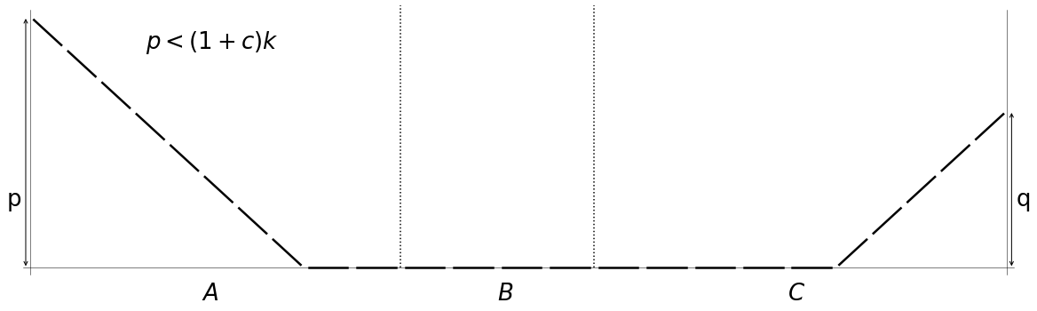
Figure 12: Division of the full chain, illustrated here at $k=8$ and $c=1/8$. A walk is schematically shown, that has too many unbalanced steps on the left for Lemma 6.5 to apply when the chain is split into equal thirds. But when splitting into unequal intervals A, B, and C, as described above, we can safely apply the approximation 6.5.

The $B$ and $C$ intervals are fully contained in the last two thirds: $B\cup C\subset[k+1,3k]$. Because of that, and the frustration-freeness of the Hamiltonian, we have

$$\langle{\phi_{p,q}}|{G_{[k+1,3k]}}|{\phi_{p,q}}\rangle\leq\langle{\phi_{p,q}}|{G_{BC}}|{\phi_{p,q}}\rangle$$ (8.26)

and it suffices to show that the term on the RHS is small. Similarly, since $G_{[1,2k]}|{\phi_{p,q}}\rangle=|{\phi_{p,q}}\rangle$ by definition of $|{\phi}\rangle$, and the left and middle intervals are contained in the first two thirds (i.e. $A\cup B\subset[1,2k]$), we have $G_{AB}|{\phi_{p,q}}\rangle=|{\phi_{p,q}}\rangle$, so we can expand $|{\phi_{p,q}}\rangle$ in terms of ground states on $A\cup B$. We will work with unnormalized such ground states, and normalize at the end.

Similarly to Section 8.2, we perform a Schmidt decomposition of $|{\phi_{p,q}}\rangle$ with respect to subsystems $A\cup B$ and $C$, in which we must include three types of terms: walks that reach zero height both within $A\cup B$ and $C$, those that do so only in $C$, and lastly those that do so only in $A\cup B$. The result is

$$|{\phi_{p,q}}\rangle={1\over\sqrt{{N^{\prime}}^{\phi}_{p,q}}}\left(\sum_{v\geq 0}|{UGS^{AB}_{p,v}}\rangle|{\psi^{C}_{v,q}}\rangle+\sum_{z=1}^{p}\sum_{v\geq 0}|{UGS^{AB}_{p-z,v}}\rangle|{{\psi^{\prime}}^{C}_{v+z,q}}\rangle+\sum_{y=1}^{q}\sum_{v\geq 0}|{UGS^{AB}_{p,v+y}}\rangle|{{\psi^{\prime\prime}}^{C}_{v,q-y}}\rangle\right)$$ (8.27)

where $|{UGS^{AB}}\rangle$ denotes an unnormalized ground state on the union of segments $A$ and $B$, while $|{\psi_{C}}\rangle$, $|{{\psi^{\prime}}^{C}}\rangle$ and $|{{\psi^{\prime\prime}}^{C}}\rangle$ are also unnormalized (having absorbed the Schmidt coefficients into their definition), and live on the $C$ segment. Although the overall normalization factor ${N^{\prime}}^{\phi}_{p,q}$ could also be absorbed in the definition of the $|{\psi}\rangle$, we prefer to keep it explicit. For the purpose of proving that the supremum of $\langle{\phi_{p,q}}|{G_{BC}}|{\phi_{p,q}}\rangle$ vanishes at large $k$, it is enough to only consider the first term above, and furthermore one can restrict the summation over $v$ to only run up to $bk$. Formally, one has:

Definition 8.6.

Given an arbitrary $|{\phi_{p,q}}\rangle\in\operatorname{range}E_{k}$, extract from the expansion (8.27) the collection of states $\{\psi^{C}_{v,q}\}$, indexed by $v$, that contribute to the first sum. We define the following substitute for the original state:

$$|{\phi_{p,q}^{\prime}}\rangle={1\over\sqrt{N^{\phi}_{p,q}}}\sum_{v<bk}|{UGS^{AB}_{p,v}}\rangle|{\psi^{C}_{v,q}}\rangle$$ (8.28)

where for normalization we need

$$N^{\phi}_{p,q}=\sum_{v<bk}\langle{UGS^{AB}_{p,v}}|{UGS^{AB}_{p,v}}\rangle\cdot\langle{\psi^{C}_{v,q}}|{\psi^{C}_{v,q}}\rangle$$ (8.29)

Since $|{\phi_{p,q}}\rangle$ is constrained to be orthogonal to the ground state on the full chain $[1,3k]$, the collections $\{\psi^{C}_{v,q}\}$ that can be obtained by the procedure above are not fully arbitrary. Let $P_{k,q}$ be the set of all such collections that can be obtained at specific $k$ and $q$.

Note that $|{\phi_{p,q}^{\prime}}\rangle$ may not always provide a ‘good approximation’ of $|{\phi_{p,q}}\rangle$, in the sense of the previous sections: as $k$ grows, the overlap of the states need not go to 1. Indeed, in eq. (8.27) one may take all the $|{\psi^{C}}\rangle$ to vanish, and use only nonzero $|{{\psi^{\prime}}^{C}}\rangle$ and $|{{\psi^{\prime\prime}}^{C}}\rangle$ instead. Then our substitute is orthogonal to the initial state. However, $|{\phi_{p,q}^{\prime}}\rangle$ is still useful for our bound as the following proposition shows.

Notation 8.7.

In the remainder of this subsection, we abbreviate

$$\lim\limits_{k\to\infty}\sup\limits_{0\leq p,q<(1+c)k}\equiv\widetilde{\lim\limits_{k\to\infty}}$$

Proposition 8.8.

Assuming both limits exist, we have

$$\widetilde{\lim\limits_{k\to\infty}}\left(\sup\limits_{|{\phi_{p,q}}\rangle\in\operatorname{range}E_{k}}\langle{\phi_{p,q}}|{G_{BC}}|{\phi_{p,q}}\rangle\right)\leq\widetilde{\lim\limits_{k\to\infty}}\left(\sup\limits_{\{\psi^{C}_{s,q}\}\in P_{k,q}}\langle{\phi_{p,q}^{\prime}}|{G_{BC}}|{\phi_{p,q}^{\prime}}\rangle\right)$$ (8.30)

The proof of Proposition 8.8 is straightforward, but the details are rather lengthy and tangential to the main argument of this section. Therefore, the discussion is deferred to Section B.8. We continue with

Definition 8.9.

Since $|{\phi_{p,q}^{\prime}}\rangle$ is written in terms of ground states on the $AB$ part of the chain, all of which have a relatively small number of unbalanced steps, to approximate it we consider

$$|{A\phi_{p,q}}\rangle={1\over\sqrt{AN^{\phi}_{p,q}}}\sum_{r,v<bk}|{UGS^{A}_{p,r}}\rangle|{UGS^{B}_{r,v}}\rangle|{\psi^{C}_{v,q}}\rangle$$ (8.31)

where normalization requires

$$AN^{\phi}_{p,q}=\sum_{r,v<bk}N^{A}_{p,r}\cdot N^{B}_{r,v}\cdot\langle{\psi^{C}_{v,q}}|{\psi^{C}_{v,q}}\rangle$$ (8.32)

Proposition 8.10.

The $|{A\phi_{p,q}}\rangle$ states of Definition 8.9 satisfy

$$\widetilde{\lim\limits_{k\to\infty}}\left(\sup\limits_{\{\psi^{C}_{v,q}\}\in P_{k,q}}\langle{\phi_{p,q}^{\prime}}|{G_{BC}}|{\phi_{p,q}^{\prime}}\rangle\right)=\widetilde{\lim\limits_{k\to\infty}}\left(\sup\limits_{\{\psi^{C}_{v,q}\}\in P_{k,q}}\langle{A\phi_{p,q}}|{G_{BC}}|{A\phi_{p,q}}\rangle\right)$$ (8.33)

Proof.

The assumptions required by Lemma B.6 clearly hold if we take $L=A\cup B$ and $R=C$. Then we apply Lemma B.12 and the proof is complete. ∎

From the classification of ground states in Section 3.1, we know that the ground space projector on BC is given by

$$G_{BC}=\sum_{r^{\prime},q^{\prime}}|{GS_{r^{\prime},q^{\prime}}^{BC}}\rangle\langle{GS_{r^{\prime},q^{\prime}}^{BC}}|$$ (8.34)

When inserting the form for $|{A\phi_{p,q}}\rangle$ from eq. (8.31) into the matrix element $\langle{A\phi_{p,q}}|{G_{BC}}|{A\phi_{p,q}}\rangle$, only $r$ values below $bk$ contribute, because the overlap $\langle{GS_{r^{\prime},q^{\prime}}^{BC}}|\;\big{(}|{UGS^{B}_{r,v}}\rangle|{\psi^{C}_{v,q}}\rangle\big{)}$ is only nonzero when $r=r^{\prime}$ and $q=q^{\prime}$. For the same reason, only $q^{\prime}$ values exactly equal to $q$ will matter.

Definition 8.11.

Guided by this observation, isolate the part of the projector that actually contributes:

$$G_{BC}^{\prime}=\sum_{r<bk}|{GS_{r,q}^{BC}}\rangle\langle{GS_{r,q}^{BC}}|$$ (8.35)

From the argument above, we find $\langle{A\phi_{p,q}}|{G_{BC}}|{A\phi_{p,q}}\rangle=\langle{A\phi_{p,q}}|{G_{BC}^{\prime}}|{A\phi_{p,q}}\rangle$. Every state in eq. (8.35) above has both $r$ and $q$ small enough that approximation Lemma 6.5 applies. The following states then superpolynomially approximate the $|{GS_{r,q}^{BC}}\rangle$ when $r<bk$ and $q<(1+c)k$:

Definition 8.12.

$$|{AGS_{r,q}^{BC}}\rangle={1\over\sqrt{AN_{r,q}^{BC}}}\sum_{v<bk}|{UGS_{r,v}^{B}}\rangle|{UGS_{v,q}^{C}}\rangle$$ (8.36)

Definition 8.13.

These states are then used to define the approximate projector:

$$AG_{BC}=\sum_{r<bk}{1\over AN_{r,q}^{BC}}\sum_{v,v^{\prime}<bk}|{UGS_{r,v}^{B}}\rangle|{UGS_{v,q}^{C}}\rangle\langle{UGS_{r,v^{\prime}}^{B}}|\langle{UGS_{v^{\prime},q}^{C}}|$$ (8.37)

According to Lemma B.16, this approximates $G_{BC}^{\prime}$, and we have

$$\widetilde{\lim\limits_{k\to\infty}}\left(\sup\limits_{\{\psi^{C}_{v,q}\}\in P_{k,q}}\langle{A\phi_{p,q}}|{G_{BC}^{\prime}}|{A\phi_{p,q}}\rangle\right)=\widetilde{\lim\limits_{k\to\infty}}\left(\sup\limits_{\{\psi^{C}_{v,q}\}\in P_{k,q}}\langle{A\phi_{p,q}}|{AG_{BC}}|{A\phi_{p,q}}\rangle\right)$$ (8.38)

Combining Propositions 8.8 and 8.10 with the above we find

$$\widetilde{\lim\limits_{k\to\infty}}\left(\sup\limits_{|{\phi_{p,q}}\rangle\in\operatorname{range}E_{k}}\langle{\phi_{p,q}}|{G_{BC}}|{\phi_{p,q}}\rangle\right)=\widetilde{\lim\limits_{k\to\infty}}\left(\sup\limits_{\{\psi^{C}_{v,q}\}\in P_{k,q}}\langle{A\phi_{p,q}}|{AG_{BC}}|{A\phi_{p,q}}\rangle\right)$$ (8.39)

Recall that the constraint $\{\psi^{C}_{v,q}\}\in P_{k,q}$ comes from the necessity that $|{\phi_{p,q}}\rangle$ is always orthogonal to the ground space on the full chain $ABC$. To describe that in a different manner, ground states on the full chain are first approximated as follows:

Definition 8.14.

For the ground state on the full chain we will use the approximation

$$|{FGS_{p,q}}\rangle={1\over\sqrt{AN_{p,q}^{ABC}}}\sum_{r,v<bk}|{UGS^{A}_{p,r}}\rangle|{UGS^{B}_{r,v}}\rangle|{UGS^{C}_{v,q}}\rangle$$ (8.40)

with the corresponding normalization factor

$$AN_{p,q}^{ABC}=\sum_{r,v<bk}N^{A}_{p,r}N^{B}_{r,v}N^{C}_{v,q}$$ (8.41)

Proposition 8.15.

The $|{FGS_{p,q}}\rangle$ of Definition 8.14 superpolynomially approximate the true ground states $|{GS^{ABC}_{p,q}}\rangle$ on the full chain, for all $p,q\leq(1+c)k$.

Proof of Proposition 8.15.

It follows directly by Lemma B.9. ∎

By construction, the state $|{FGS_{p,q}}\rangle$ only contains walks that simultaneously reach zero height in all three segments $A,B,C$. Therefore, when computing an overlap such as $\langle{FGS_{p,q}}|{\phi_{p,q}}\rangle$, only walks with the same property will be picked out within $|{\phi_{p,q}}\rangle$. These are precisely the walks that have been included in the substitute state $|{\phi_{p,q}^{\prime}}\rangle$; moreover, these walks have the same relative prefactors in $|{\phi_{p,q}^{\prime}}\rangle$ as they did in $|{\phi_{p,q}}\rangle$. The only possible difference is in the absolute values of the prefactors, which may occur because we imposed that $|{\phi_{p,q}^{\prime}}\rangle$ has norm 1, while the corresponding component within $|{\phi_{p,q}}\rangle$ may have subunitary norm. However, in eq. (8.42) below we are taking the supremum on both sides, which for $|{\phi_{p,q}}\rangle$ will occur when no $|{{\psi^{\prime}}^{C}}\rangle$ or $|{{\psi^{\prime\prime}}^{C}}\rangle$ components are present. Then, the absolute values of the prefactors are also identical, and equality between the LHS and RHS below follows:

$$\widetilde{\lim\limits_{k\to\infty}}\left(\sup\limits_{|{\phi_{p,q}}\rangle\in\operatorname{range}E_{k}}|\langle{FGS_{p,q}}|{\phi_{p,q}}\rangle|\right)=\widetilde{\lim\limits_{k\to\infty}}\left(\sup\limits_{\{\psi^{C}_{v,q}\}\in P_{k,q}}|\langle{FGS_{p,q}}|{\phi_{p,q}^{\prime}}\rangle|\right)$$ (8.42)

Since the true $|{\phi_{p,q}}\rangle$ must be orthogonal to the true ground state $|{GS_{p,q}^{ABC}}\rangle$, we use Lemma B.12 twice to find that the overlap of their approximations also vanishes:

$$0 =\widetilde{\lim\limits_{k\to\infty}}\left(\sup\limits_{|{\phi_{p,q}}\rangle\in\operatorname{range}E_{k}}|\langle{GS_{p,q}^{ABC}}|{\phi_{p,q}}\rangle|\right)=\widetilde{\lim\limits_{k\to\infty}}\left(\sup\limits_{|{\phi_{p,q}}\rangle\in\operatorname{range}E_{k}}|\langle{FGS_{p,q}}|{\phi_{p,q}}\rangle|\right)$$

$$=\widetilde{\lim\limits_{k\to\infty}}\left(\sup\limits_{\{\psi^{C}_{v,q}\}\in P_{k,q}}|\langle{FGS_{p,q}}|{\phi_{p,q}^{\prime}}\rangle|\right)=\widetilde{\lim\limits_{k\to\infty}}\left(\sup\limits_{\{\psi^{C}_{v,q}\}\in P_{k,q}}|\langle{FGS_{p,q}}|{A\phi_{p,q}}\rangle|\right)$$

The overlap on the last line can be computed at any particular $(p,q)$:

$$\langle{FGS_{p,q}}|{A\phi_{p,q}}\rangle=\sum_{r,r^{\prime},v,v^{\prime}<bk}\frac{\Big{(}\langle{UGS^{A}_{p,r^{\prime}}}|\langle{UGS^{B}_{r^{\prime},v^{\prime}}}|\langle{UGS^{C}_{v^{\prime},q}}|\Big{)}\Big{(}|{UGS^{A}_{p,r}}\rangle|{UGS^{B}_{r,v}}\rangle|{\psi^{C}_{v,q}}\rangle\Big{)}}{\sqrt{AN^{\phi}_{p,q}\cdot AN^{ABC}_{p,q}}}$$ (8.43)

In order to have any overlap, states must have identical numbers of unbalanced steps. Recalling from Theorem 2.4 and the definition of the unnormalized ground states that

$$\langle{UGS^{i}_{a^{\prime},b^{\prime}}}|{UGS^{i}_{a,b}}\rangle=N^{i}_{a,b}\cdot\delta_{a,a^{\prime}}\cdot\delta_{b,b^{\prime}}\quad\quad\forall i\in\{A,B,C\}$$ (8.44)

one obtains for the above

$$\langle{FGS_{p,q}}|{A\phi_{p,q}}\rangle ={1\over\sqrt{AN^{\phi}_{p,q}\cdot AN_{p,q}}}\sum_{r,v<bk}N^{A}_{p,r}N^{B}_{r,v}\cdot\langle{UGS^{C}_{v,q}}|{\psi^{C}_{v,q}}\rangle$$ (8.45)

A similar computation can be performed for the matrix element $\langle{A\phi_{p,q}}|{AG_{BC}}|{A\phi_{p,q}}\rangle$:

$$\langle{A\phi_{p,q}}|{AG_{BC}}|{A\phi_{p,q}}\rangle={1\over AN^{\phi}_{p,q}}\sum_{r_{1},v_{1},r_{2},v_{2},r,v,v^{\prime}} {1\over AN_{r,q}^{BC}}\cdot\langle{UGS^{A}_{p,r_{1}}}|{UGS^{A}_{p,r_{2}}}\rangle\cdot\langle{UGS^{B}_{r_{1},v_{1}}}|{UGS^{B}_{r,v}}\rangle$$

$$\cdot\langle{UGS^{B}_{r,v^{\prime}}}|{UGS^{B}_{r_{2},v_{2}}}\rangle\cdot\langle{\psi^{C}_{v_{1},q}}|{UGS^{C}_{v,q}}\rangle\cdot\langle{UGS^{C}_{v^{\prime},q}}|{\psi^{C}_{v_{2},q}}\rangle$$

which, taking care of all delta functions that effectively remove some summation variables, gives

$$\langle{A\phi_{p,q}}|{AG_{BC}}|{A\phi_{p,q}}\rangle ={1\over AN^{\phi}_{p,q}}\sum_{v_{1},v_{2},r}{1\over AN_{r,q}^{BC}}\cdot N^{A}_{p,r}\cdot N^{B}_{r,v_{1}}\cdot N^{B}_{r,v_{2}}\cdot\langle{\psi^{C}_{v_{1},q}}|{UGS^{C}_{v_{1},q}}\rangle\cdot\langle{UGS^{C}_{v_{2},q}}|{\psi^{C}_{v_{2},q}}\rangle$$ (8.46)

$$={1\over AN^{\phi}_{p,q}}\sum_{r}{N^{A}_{p,r}\over AN_{r,q}^{BC}}\cdot\left(\sum_{v_{1}}N^{B}_{r,v_{1}}\cdot\langle{\psi^{C}_{v_{1},q}}|{UGS^{C}_{v_{1},q}}\rangle\right)\cdot\left(\sum_{v_{2}}N^{B}_{r,v_{2}}\cdot\langle{UGS^{C}_{v_{2},q}}|{\psi^{C}_{v_{2},q}}\rangle\right)$$ (8.47)

In both (8.45) and (8.47) we can see that any component of $|{\psi^{C}_{v,q}}\rangle$ not in the ground space of the Hamiltonian acting on $C$ contributes nothing to the numerator, while making the normalization factor $AN^{\phi}_{p,q}$ in the denominator larger. Therefore it is advantageous to separate the component of $|{\psi^{C}_{v,q}}\rangle$ in the ground space corresponding to $C$:

Definition 8.16.

For every initial $|{\phi_{p,q}}\rangle$, let $\{c_{v}\}$ be the collection, indexed by $v$, of overlaps between $|{\psi^{C}_{v,q}}\rangle$ and the relevant (unnormalized) ground state:

$$c_{v}=\langle{UGS^{C}_{v,q}}|{\psi^{C}_{v,q}}\rangle$$ (8.48)

The above allows us to write

$$|{\psi^{C}_{v,q}}\rangle=c_{v}\cdot|{UGS^{C}_{v,q}}\rangle+\left(p_{v}\sqrt{N_{v,q}^{C}}\right)\cdot|{\chi_{v,q}^{C}}\rangle$$ (8.49)

where $|{\chi_{v,q}^{C}}\rangle$ is a normalized state, orthogonal to the ground space on segment $C$, and $p_{v}$ is a complex number giving the relative amplitude of $|{\chi_{v,q}^{C}}\rangle$. The square root of the normalization factor $N_{v,q}^{C}$ is conveniently chosen such that

$$\langle{\psi^{C}_{v,q}}|{\psi^{C}_{v,q}}\rangle=|c_{v}|^{2}\cdot\langle{UGS^{C}_{v,q}}|{UGS^{C}_{v,q}}\rangle+|p_{v}|^{2}\cdot N_{v,q}^{C}\cdot 1=N_{v,q}^{C}\cdot\left(|c_{v}|^{2}+|p_{v}|^{2}\right)$$ (8.50)

The only place where this appears is the approximate normalization factor of $\phi$:

$$AN^{\phi}_{p,q}=\sum_{r,v<bk}N^{A}_{p,r}\cdot N^{B}_{r,v}\cdot N_{v,q}^{C}\cdot\left(|c_{v}|^{2}+|p_{v}|^{2}\right)$$ (8.51)

With this definition, equation (8.45) becomes

$$|\langle{FGS_{p,q}}|{A\phi_{p,q}}\rangle|={1\over\sqrt{AN^{\phi}_{p,q}\cdot AN_{p,q}}}\cdot\bigg{|}\sum_{r,v<bk}N^{A}_{p,r}\cdot N^{B}_{r,v}\cdot N^{C}_{v,q}\cdot c_{v}\bigg{|}$$ (8.52)

and the matrix element that we’re looking to bound in the end is

$$\langle{A\phi_{p,q}}|{AG_{BC}}|{A\phi_{p,q}}\rangle={1\over AN^{\phi}_{p,q}}\sum_{r}{N^{A}_{p,r}\over AN_{r,q}^{BC}}\cdot\bigg{|}\sum_{v}N^{B}_{r,v}\cdot N^{C}_{v,q}\cdot c_{v}\bigg{|}^{2}$$ (8.53)

The purpose is to bound the supremum of the RHS in eq. (8.53) over all collections of factors $\{c_{v},p_{v}\}$ that could be obtained from an initial $|{\phi_{p,q}}\rangle\in\operatorname{range}E_{k}$, as described above. By the (approximate) orthogonality condition, we are guaranteed that the RHS of eq. (8.52) vanishes at large $k$, for all such obtainable collections. Therefore, the vanishing of (8.52) at large $k$ is a weaker condition than the obtainability of $\{c_{v},p_{v}\}$. In what follows we will prove that the quantity in (8.53) vanishes at large $k$ even only under this weaker condition, which will also prove the desired result. The approximate orthogonality says that

$$\widetilde{\lim\limits_{k\to\infty}}\left(\sup\limits_{\{c_{v},p_{v}\}\text{ obtainable}}{1\over\sqrt{AN^{\phi}_{p,q}\cdot AN_{p,q}}}\cdot\bigg{|}\sum_{r,v<bk}N^{A}_{p,r}\cdot N^{B}_{r,v}\cdot N^{C}_{v,q}\cdot c_{v}\bigg{|}\right)=0$$ (8.54)

As discussed above, the condition that $\{c_{v},p_{v}\}$ must be obtainable will be relaxed, and replaced by the weaker condition that the above limit vanishes. Going on, we will also abbreviate $\{c_{v},p_{v}\}$ by $\{\tilde{c}_{v}\}$ (since the $p_{v}$ are unimportant). When writing $\sup_{\{\tilde{c}_{v}\}}$ we mean the supremum over all collections $\{c_{v},p_{v}\}$ which obey the vanishing condition. We are looking to bound, in the limit of large $k$, the following:

$$\sup\limits_{0\leq p,q\leq(1+c)k}\left(\sup\limits_{\{\tilde{c}_{v}\}}\Big{(}\langle{A\phi_{p,q}}|{AG_{BC}}|{A\phi_{p,q}}\rangle\Big{)}\right)$$ (8.55)

$$= \sup\limits_{0\leq p,q\leq(1+c)k}\left(\sup\limits_{\{\tilde{c}_{v}\}}\left({1\over AN^{\phi}_{p,q}}\sum_{r}{N^{A}_{p,r}\over AN_{r,q}^{BC}}\cdot\bigg{|}\sum_{s}N^{B}_{r,v}\cdot N^{C}_{v,q}\cdot c_{v}\bigg{|}^{2}\right)\right)$$

Definition 8.17.

The following quantities are convenient:

$$x_{r}^{(k,\{\tilde{c}_{v}\})}\equiv{\sum_{s}N_{r,v}^{B}\cdot N_{v,q}^{C}\cdot c_{v}\over AN^{BC}_{r,q}}\cdot\sqrt{AN_{p,q}\over AN^{\phi}_{p,q}}$$ (8.56)

where the $p,q$ dependence of the $x_{r}$ factors is kept implicit. We can simplify the expression by also defining

$$j^{(k,\{\tilde{c}_{v}\})}_{p,q}=\sqrt{AN_{p,q}\over AN^{\phi}_{p,q}}=\sqrt{\sum_{u,v}N_{p,u}^{A}\cdot N_{u,v}^{B}\cdot N_{v,q}^{C}\over\sum_{u,v}N_{p,u}^{A}\cdot N_{u,v}^{B}\cdot N_{v,q}^{C}\cdot|c_{v}|^{2}}$$ (8.57)

and the ratios

$$\pi^{(k)}_{r,v}={N_{r,v}^{B}\over N_{0,v}^{B}}$$ (8.58)

Writing $AN^{BC}_{r,q}$ as a sum, we obtain

$$x_{r}\equiv{\sum_{v}\pi_{r,v}\cdot N_{0,v}^{B}\cdot N_{v,q}^{C}\cdot c_{v}\over\sum_{v}\pi_{r,v}\cdot N_{0,v}^{B}\cdot N_{v,q}^{C}}\cdot j_{p,q}$$ (8.59)

Note that the $x_{r}$ are invariant (up to a global phase) under an uniform scaling $c_{v}\to a\cdot c_{v}$ and $p_{v}\to a\cdot p_{v}$ (fixed $a\in\mathbb{C}$, for all $v$ simultaneously), i.e. they only depend on the relations among the various $c_{v},p_{v}$ and not their overall magnitudes (as it should be, since the $c_{v},p_{v}$ were defined as part of an unnormalized expression). This definition is convenient because eq. (8.52) becomes

$$|\langle{FGS_{p,q}}|{A\phi_{p,q}}\rangle|=\bigg{|}\sum_{r}{N^{A}_{p,r}\cdot AN^{BC}_{r,q}\over AN_{p,q}}\cdot x_{r}\bigg{|}$$ (8.60)

while eq. (8.53) turns into

$$\langle{A\phi_{p,q}}|{AG_{BC}}|{A\phi_{p,q}}\rangle=\sum_{r}{N^{A}_{p,r}\cdot AN^{BC}_{r,q}\over AN_{p,q}}\cdot|x_{r}|^{2}$$ (8.61)

with the convenient property that, in both of the above, the coefficients in front of the $x_{r}$ sum to 1, by construction:

$$\sum_{r}{N^{A}_{p,r}\cdot AN^{BC}_{r,q}\over AN_{p,q}}={\sum_{r}N^{A}_{p,r}\cdot AN^{BC}_{r,q}\over AN_{p,q}}={\sum_{r}N^{A}_{p,r}\cdot AN^{BC}_{r,q}\over\sum_{r}N^{A}_{p,r}\cdot AN^{BC}_{r,q}}=1$$ (8.62)

The key must be in how the various $x_{r}$ relate to each other. The only $r$ dependence is in the $\pi_{r,v}$ factors, present both in the numerator and denominator of eq. (8.59).

As we will see in the following section, at large $k$, the quantity $\pi_{r,v}$ depends very weakly on $v$, allowing us to show that the $x_{r}$ factors with various $r$ are very close to each other; and from that, we will prove that prove that the quantity in eq. (8.61) becomes very small at large $k$.

9 Normalizations and the $x_{r}$ factors

In this rather technical section we show that the relevant $x_{r}$ factors approach $r$-independent quantities at large $k$:

Lemma 9.1.

With Definition 8.17 and the condition (8.54) constraining the $\{\tilde{c}_{s}\}$ factors, we have that

$$\lim\limits_{k\to\infty}\left(\sup\limits_{0\leq p,q\leq(1+c)k}\left(\sup\limits_{\{\tilde{c}_{v}\}}\left(\sup\limits_{r<bk}|x_{r}^{(k,\{\tilde{c}_{v}\})}-x_{0}^{(k,\{\tilde{c}_{v}\})}|\right)\right)\right)=0$$ (9.1)

Before proving Lemma 9.1, we rephrase the main result of Appendix A:

Proposition 9.2.

Make the notation $\pi_{r}\equiv\pi_{r,0}$. For any $\epsilon>0$, there exists a $k_{0}$ such that for all $k>k_{0}$ the following holds true:

$$\forall r,v<bk\quad\text{we have}\quad 0\leq 1-{\pi_{r,v}\over\pi_{r}}<\epsilon$$ (9.2)

Proof of Proposition 9.2.

We know from Theorem A.2 that, given the value of $t$, there exist constants $C_{*},\alpha,\beta>0$ such that for all $r+v\leq k$,

$$0\leq\pi_{r}-\pi_{r,v}^{(k)}\leq C_{*}t^{\alpha(k-\beta r-\beta v)}\pi_{r}\quad\iff\quad 0\leq 1-{\pi_{r,v}^{(k)}\over\pi_{r}}\leq C_{*}t^{\alpha[k-\beta(r+v)]}$$ (9.3)

When imposing $r,v<bk$ we find that

$$k-\beta(r+v)>k-\beta\cdot 2bk=k\cdot(1-2\beta b)$$ (9.4)

This is where the condition $b<{1\over 4\beta}$ from Assumption 6.2 plays an important role: with this constraint on $b$, we find that the rightmost term above is above $k(1-1/2)=k/2$. With $\alpha>0$ and $t<1$, we find that

$$t^{\alpha[k-\beta(r+v)]}<t^{\alpha k/2}$$ (9.5)

and so it follows that

$$0\leq 1-{\pi_{r,v}^{(k)}\over\pi_{r}}<C_{*}t^{\alpha k/2}$$ (9.6)

For the desired inequality (9.2) to hold, it is clear that it is sufficient to take $k$ large enough such that

$$C_{*}t^{\alpha k/2}\stackrel{{\scriptstyle!}}{{<}}\epsilon$$ (9.7)

Due to the positivity of all relevant constants, and the fact that $t<1$, this is satisfied if

$$k>{2\over\alpha}\cdot{\ln\left({\epsilon/C_{*}}\right)\over\ln t}$$ (9.8)

which shows that a suitable $k_{0}$ can indeed be chosen, completing the proof. ∎

We now turn to proving the main result of the section:

Proof of Lemma 9.1.

Fix some small $\epsilon>0$, and using Proposition 9.2, take $k$ large enough such that

$$\forall r,v<bk\quad\text{we have}\quad 0\leq 1-{\pi_{r,v}\over\pi_{r}}<\epsilon$$ (9.9)

where, for simplicity, the $k$ dependence of the $\pi_{r,v}^{(k)}$ terms is suppressed. This is equivalent to

$$\forall r,v<bk\quad\text{we have}\quad 0\leq\pi_{r}-\pi_{r,v}<\epsilon\pi_{r}\quad\iff\quad\pi_{r}\geq\pi_{r,v}>\pi_{r}\cdot(1-\epsilon)$$ (9.10)

Take arbitrary, but specific $p,q$ obeying the condition of the lemma, and a collection of complex $\{\tilde{c}_{v}\}$ obeying the constraint (8.54). We separate the real and imaginary parts of the $c_{v}$ factors, so write $c_{v}=d_{v}+ie_{v}$ where $d_{v},e_{v}\in\mathbb{R}$ for all $v$. Some of the $\{d_{v}\}$ and $\{e_{v}\}$ may be positive, and some may be negative. We define accordingly

Definition 9.3.

$$x_{r}^{+}={\sum_{v;\;d_{v}>0}\pi_{r,v}\cdot N_{0,v}^{B}\cdot N_{v,q}^{C}\cdot|d_{v}|\over\sum_{v}\pi_{r,v}\cdot N_{0,v}^{B}\cdot N_{v,q}^{C}}\cdot j_{p,q}\qquad \qquad x_{r}^{-}={\sum_{v;\;d_{v}<0}\pi_{r,v}\cdot N_{0,v}^{B}\cdot N_{v,q}^{C}\cdot|d_{v}|\over\sum_{v}\pi_{r,v}\cdot N_{0,v}^{B}\cdot N_{v,q}^{C}}\cdot j_{p,q}$$ (9.11)

$$y_{r}^{+}={\sum_{v;\;e_{v}>0}\pi_{r,v}\cdot N_{0,v}^{B}\cdot N_{v,q}^{C}\cdot|e_{v}|\over\sum_{v}\pi_{r,v}\cdot N_{0,v}^{B}\cdot N_{v,q}^{C}}\cdot j_{p,q}\qquad \qquad y_{r}^{-}={\sum_{v;\;e_{v}<0}\pi_{r,v}\cdot N_{0,v}^{B}\cdot N_{v,q}^{C}\cdot|e_{v}|\over\sum_{v}\pi_{r,v}\cdot N_{0,v}^{B}\cdot N_{v,q}^{C}}\cdot j_{p,q}$$ (9.12)

the partial sums including only positive or only negative terms in the numerator of the fraction, such that $x_{r}^{+},x_{r}^{-},y_{r}^{+},y_{r}^{-}>0$ and $x_{r}=\big{(}x_{r}^{+}-x_{r}^{-}\big{)}+i\big{(}y_{r}^{+}-y_{r}^{-}\big{)}$.

We will prove that $x_{r}^{\pm}$ is close to $x_{0}^{\pm}$, and the same for the $y^{\pm}_{r}$ and $y^{\pm}_{0}$ factors. This will then show that $x_{r}$ is close to $x_{0}$. To begin, we will only work with the $x_{r}^{\pm}$. Since $\pi_{r,v}\leq\pi_{r}$, the denominator of all the fractions above is bounded by

$$\sum_{v}\pi_{r,v}\cdot N_{0,v}^{B}\cdot N_{v,q}^{C}\leq\pi_{r}\sum_{v}N_{0,v}^{B}\cdot N_{v,q}^{C}\quad\implies\quad{1\over\sum_{v}\pi_{r,v}\cdot N_{0,v}^{B}\cdot N_{v,q}^{C}}\geq{1\over\pi_{r}}\cdot{1\over\sum_{v}N_{0,v}^{B}\cdot N_{v,q}^{C}}$$ (9.13)

Moving the $1/\pi_{r}$ factor up to the numerator of the fraction, we get

$$x_{r}^{+}\geq{\sum_{v;\;d_{v}>0}{\pi_{r,v}\over\pi_{r}}\cdot N_{0,v}^{B}\cdot N_{v,q}^{C}\cdot|d_{v}|\over\sum_{v}N_{0,v}^{B}\cdot N_{v,q}^{C}}\cdot j_{p,q}$$ (9.14)

Observing that

$$x_{0}^{+}={\sum_{v;\;d_{v}>0}N_{0,v}^{B}\cdot N_{v,q}^{C}\cdot|d_{v}|\over\sum_{v}N_{0,v}^{B}\cdot N_{v,q}^{C}}\cdot j_{p,q}$$ (9.15)

and from the normalization ratio convergence assumption

$${\pi_{r,v}\over\pi_{r}}>1-\epsilon$$ (9.16)

together with the fact that all the terms $N_{0,v}^{B}\cdot N_{v,q}^{C}\cdot|d_{v}|$ in the numerator sum are positive, we find

$$x_{r}^{+}>{\sum_{v;\;d_{v}>0}{\pi_{r,v}\over\pi_{r}}\cdot N_{0,v}^{B}\cdot N_{v,q}^{C}\cdot|d_{v}|\over\sum_{v}N_{0,v}^{B}\cdot N_{v,q}^{C}}\cdot j_{p,q}>{\sum_{v;\;d_{v}>0}(1-\epsilon)\cdot N_{0,v}^{B}\cdot N_{v,q}^{C}\cdot|d_{v}|\over\sum_{v}N_{0,v}^{B}\cdot N_{v,q}^{C}}\cdot j_{p,q}=(1-\epsilon)\cdot x_{0}^{+}$$ (9.17)

and by an identical argument $x_{r}^{-}>(1-\epsilon)\cdot x_{0}^{-}$. For the corresponding upper bounds we again start with the denominators

$$\sum_{v}\pi_{r,v}\cdot N_{0,v}^{B}\cdot N_{v,q}^{C}>\pi_{r}(1-\epsilon)\sum_{v}N_{0,v}^{B}\cdot N_{v,q}^{C}\;\implies\;{1\over\sum_{v}\pi_{r,v}\cdot N_{0,v}^{B}\cdot N_{v,q}^{C}}<{1\over 1-\epsilon}\cdot{1\over\pi_{r}}\cdot{1\over\sum_{v}N_{0,v}^{B}\cdot N_{v,q}^{C}}$$ (9.18)

and with ${\pi_{r,v}/\pi_{r}}\leq 1$ we see

$$x_{r}^{+}<{1\over 1-\epsilon}\cdot{\sum_{v;\;d_{v}>0}{\pi_{r,v}\over\pi_{r}}\cdot N_{0,v}^{B}\cdot N_{v,q}^{C}\cdot|d_{v}|\over\sum_{v}N_{0,v}^{B}\cdot N_{v,q}^{C}}\cdot j_{p,q}\leq{1\over 1-\epsilon}\cdot{\sum_{v;\;d_{v}>0}N_{0,v}^{B}\cdot N_{v,q}^{C}\cdot|d_{v}|\over\sum_{v}N_{0,v}^{B}\cdot N_{v,q}^{C}}\cdot j_{p,q}={1\over 1-\epsilon}\cdot x_{0}^{+}$$ (9.19)

and similarly $x_{r}^{-}<x_{0}^{-}/(1-\epsilon)$. For convenience we observe

$${1\over 1-\epsilon}=\sum_{n=0}^{\infty}\epsilon^{n}=1+\epsilon+\epsilon^{2}\cdot\sum_{n=0}^{\infty}\epsilon^{n}=1+\epsilon+\epsilon\cdot{\epsilon\over 1-\epsilon}$$ (9.20)

and taking $\epsilon$ small enough that ${\epsilon\over 1-\epsilon}<1$, we find ${1\over 1-\epsilon}<1+2\epsilon$. This gives

$$(1-\epsilon)\cdot x_{0}^{\pm}<x_{r}^{\pm}<(1+2\epsilon)\cdot x_{0}^{\pm}$$ (9.21)

For symmetry purposes, use $1-\epsilon>1-2\epsilon$ and write

$$(1-2\epsilon)\cdot x_{0}^{\pm}<x_{r}^{\pm}<(1+2\epsilon)\cdot x_{0}^{\pm}$$ (9.22)

which gives a lower bound on the difference $x_{r}^{+}-x_{r}^{-}$ of

$$x_{r}^{+}-x_{r}^{-}>(1-2\epsilon)x_{0}^{+}-(1+2\epsilon)x_{0}^{-}=(x_{0}^{+}-x_{0}^{-})-2\epsilon(x_{0}^{+}+x_{0}^{-})$$ (9.23)

Recalling from the definitions above that the real part of $x_{r}$ is $x_{r}^{+}-x_{r}^{-}$, we see that the above reads $\Re(x_{r})>\Re(x_{0})-2\epsilon(x_{0}^{+}+x_{0}^{-})$. The upper bound gives similarly $\Re(x_{r})<\Re(x_{0})+2\epsilon(x_{0}^{+}+x_{0}^{-})$, so we have

$$|\Re(x_{r}-x_{0})|<2\epsilon(x_{0}^{+}+x_{0}^{-})$$ (9.24)

To complete the argument, we need to find a bound on $x_{0}^{+}+x_{0}^{-}$. We start by examining the square of the quantity $j_{p,q}$ defined in 8.17 above:

$$j_{p,q}^{2}={\sum_{u,v}N_{p,u}^{A}\cdot N_{u,v}^{B}\cdot N_{v,q}^{C}\over\sum_{u,v}N_{p,u}^{A}\cdot N_{u,v}^{B}\cdot N_{v,q}^{C}\cdot\left(|c_{v}|^{2}+|p_{v}^{2}|\right)}={\sum_{u,v}N_{p,u}^{A}\cdot\pi_{u,v}\cdot N_{0,v}^{B}\cdot N_{v,q}^{C}\over\sum_{u,v}N_{p,u}^{A}\cdot\pi_{u,v}\cdot N_{0,v}^{B}\cdot N_{v,q}^{C}\cdot\left(|c_{v}|^{2}+|p_{v}^{2}|\right)}$$ (9.25)

All the terms in the sums above are positive, so we can safely use the bounds $\pi_{u,v}\leq\pi_{u}$ in the numerator and $\pi_{u,v}>(1-\epsilon)\pi_{u}$ in the denominator, to bound $j_{p,q}^{2}$ from above. Then the $u$ sums cancel and we obtain

$$j_{p,q}<\sqrt{1\over 1-\epsilon}\cdot\sqrt{\sum_{v}N_{0,v}^{B}\cdot N_{v,q}^{C}\over\sum_{v}N_{0,v}^{B}\cdot N_{v,q}^{C}\cdot\left(|c_{v}|^{2}+|p_{v}^{2}|\right)}$$ (9.26)

The quantity $x_{0}^{+}+x_{0}^{-}$ is related to the real parts of all the $c_{v}$ coefficients, so we will retain only that part of the bound. We also discard the unimportant $p_{v}$ factors. Namely, by using $|c_{v}|^{2}=|d_{v}|^{2}+|e_{v}|^{2}$ and the fact that all the terms in the denominator are positive, we keep

$$j_{p,q}<\sqrt{1\over 1-\epsilon}\cdot\sqrt{\sum_{v}N_{0,v}^{B}\cdot N_{v,q}^{C}\over\sum_{v}N_{0,v}^{B}\cdot N_{v,q}^{C}\cdot|d_{v}|^{2}}$$ (9.27)

Of course, it also holds true by the same token (and would be useful if we were discussing the $y_{r}^{\pm}$ factors) that we have a bound involving the imaginary parts of the $\{\tilde{c}_{v}\}$ coefficients:

$$j_{p,q}<\sqrt{1\over 1-\epsilon}\cdot\sqrt{\sum_{v}N_{0,v}^{B}\cdot N_{v,q}^{C}\over\sum_{v}N_{0,v}^{B}\cdot N_{v,q}^{C}\cdot|e_{v}|^{2}}$$ (9.28)

From the definitions (9.11) together with $\pi_{0,v}\equiv 1$ we see that

$$x_{0}^{+}+x_{0}^{-}={\sum_{v}N_{0,v}^{B}\cdot N_{v,q}^{C}\cdot|d_{v}|\over\sum_{v}N_{0,v}^{B}\cdot N_{v,q}^{C}}\cdot j_{p,q}<{\sum_{v}N_{0,v}^{B}\cdot N_{v,q}^{C}\cdot|d_{v}|\over\sum_{v}N_{0,v}^{B}\cdot N_{v,q}^{C}}\cdot\sqrt{1\over 1-\epsilon}\cdot\sqrt{\sum_{v}N_{0,v}^{B}\cdot N_{v,q}^{C}\over\sum_{v}N_{0,v}^{B}\cdot N_{v,q}^{C}\cdot|d_{v}|^{2}}$$ (9.29)

where the inequality holds due to the bound on $j_{p,q}$, and the fact that all terms multiplying it are positive. Equivalently,

$$x_{0}^{+}+x_{0}^{-}<\sqrt{1\over 1-\epsilon}\cdot\sqrt{\left(\sum_{v}N_{0,v}^{B}\cdot N_{v,q}^{C}\cdot|d_{v}|\right)^{2}\over\left(\sum_{v}N_{0,v}^{B}\cdot N_{v,q}^{C}\right)\cdot\left(\sum_{v}N_{0,v}^{B}\cdot N_{v,q}^{C}\cdot|d_{v}|^{2}\right)}$$ (9.30)

Applying Cauchy-Schwarz with terms of the form $\sqrt{N_{0,v}^{B}\cdot N_{v,q}^{C}}$ and $\sqrt{N_{0,v}^{B}\cdot N_{v,q}^{C}}\cdot|d_{v}|$ gives that the square root is at most 1. We find

$$x_{0}^{+}+x_{0}^{-}<\sqrt{1\over 1-\epsilon}\quad\implies\quad|\Re(x_{r}-x_{0})|<{2\epsilon\over\sqrt{1-\epsilon}}$$ (9.31)

It is clear that exactly the same argument carries over for the imaginary part if we replace $x_{r}^{\pm}$ by $y_{r}^{\pm}$ and the real parts of the coefficients, $d_{v}$, by the imaginary ones, $e_{v}$. We then obtain the corresponding bound $|\Im(x_{r}-x_{0})|<{2\epsilon\over\sqrt{1-\epsilon}}$, which in the end gives

$$|x_{r}-x_{0}|<{2\sqrt{2}\cdot\epsilon\over\sqrt{1-\epsilon}}$$ (9.32)

which becomes arbitrarily small when we take $\epsilon\to 0$, as desired. ∎

10 Completing the low-imbalance proof

The goal of this section is to combine the previous results and conclude that the quantity of eq. (8.53), or equivalently (8.61), goes to zero in the limit of large $k$. The argument consists of two steps:

Lemma 10.1.

The absolute values of all $x_{r}$ factors of interest vanish as $k\to\infty$. Formally,

$$\lim\limits_{k\to\infty}\left(\sup\limits_{0\leq p,q\leq(1+c)k}\left(\sup\limits_{\{\tilde{c}_{v}\}}\left(\sup\limits_{r<bk}|x_{r}^{(k,\{\tilde{c}_{v}\})}|\right)\right)\right)=0$$ (10.1)

Lemma 10.2.

In the low imbalance limit, the quantity $\langle{A\phi_{p,q}}|{AG_{BC}}|{A\phi_{p,q}}\rangle$ of eq. (8.61) vanishes at large $k$:

$$\lim\limits_{k\to\infty}\left(\sup\limits_{0\leq p,q\leq(1+c)k}\left(\sup\limits_{\{\tilde{c}_{v}\}}\left(\sum_{r<bk}{N^{A}_{p,r}\cdot AN^{BC}_{r,q}\over AN_{p,q}}\cdot|x_{r}|^{2}\right)\right)\right)=0$$ (10.2)

Proof of Lemma 10.1.

Take any $\epsilon>0$, and using the approximate orthogonality (eq. (8.54)) pick $k_{1}$ large enough such that for all $k>k_{1}$ we have

$$|\langle{FGS_{p,q}}|{A\phi_{p,q}}\rangle|=\bigg{|}\sum_{r}{N^{A}_{p,r}\cdot AN^{BC}_{r,q}\over AN_{p,q}}\cdot x_{r}\bigg{|}<{\epsilon\over 6}$$ (10.3)

where the $k$ dependence in various quantities above has been kept implicit for notational simplicity.

Definition 10.3.

For brevity make the following notation:

$$f_{r}\equiv{N^{A}_{p,r}\cdot AN^{BC}_{r,q}\over AN_{p,q}}$$ (10.4)

These $f_{r}$ factors implicitly depend on $k$, $p$, and $q$, but for now we’ll only keep the $r$ dependence explicit. Recall that $\sum_{r}f_{r}=1$ by the definition of the denominator $AN_{p,q}$.

With this notation, the above becomes

$$|\langle{FGS_{p,q}}|{A\phi_{p,q}}\rangle|=\bigg{|}\sum_{r}f_{r}\cdot x_{r}\bigg{|}<{\epsilon\over 6}$$ (10.5)

Using the result of Lemma 9.1, take $k_{2}$ large enough such that for all $k>k_{2}$ it is true that

$$\sup\limits_{0\leq p,q\leq(1+c)k}\left(\sup\limits_{\{\tilde{c}_{v}\}}\left(\sup\limits_{r<bk}|x_{r}^{(k,\{\tilde{c}_{v}\})}-x_{0}^{(k,\{\tilde{c}_{v}\})}|\right)\right)<{\epsilon\over 6}$$ (10.6)

For the rest of this proof work with $k>k_{1},k_{2}$, such that both (10.5) and (10.6) hold. Also take any $r<bk$. We will deal with the real and imaginary parts of $x_{r}$ separately. Since the absolute value of $x_{r}-x_{0}$ is below $\epsilon/6$, its real part will satisfy the same property:

$$\left|\Re(x_{r}-x_{0})\right|<{\epsilon\over 6}\quad\implies\quad\Re(x_{0})-{\epsilon\over 6}<\Re(x_{r})<\Re(x_{0})+{\epsilon\over 6}$$ (10.7)

Since all $f_{r}$ are positive, we multiply the above by $f_{r}$ and sum over $r$ (remembering $\sum_{r}f_{r}=1$) to find

$$\sum_{r}f_{r}\left(\Re(x_{0})-{\epsilon\over 6}\right)<\sum_{r}f_{r}\Re(x_{r})<\sum_{r}f_{r}\left(\Re(x_{0})+{\epsilon\over 6}\right)\quad$$ (10.8)

and so

$$\Re(x_{0})-{\epsilon\over 6}<\sum_{r}f_{r}\Re(x_{r})<\Re(x_{0})+{\epsilon\over 6}$$ (10.9)

There are three possible cases, depending on the signs of the quantities $\Re(x_{0})-{\epsilon\over 6}$ and $\Re(x_{0})+{\epsilon\over 6}$ above. If they have the same sign, be it positive or negative, we get to the same conclusion:

$${\epsilon\over 6}>|\sum_{r}f_{r}x_{r}|>|\Re(x_{0})|-{\epsilon\over 6}\quad\implies\quad|\Re(x_{0})|<{\epsilon\over 3}$$ (10.10)

while if they have opposite signs we directly get $|\Re(x_{0})|<\epsilon/6<\epsilon/3$. Combined with the property that $|\Re(x_{r}-x_{0})|<{\epsilon/6}$, we find through the triangle inequality that $|\Re(x_{r})|<\epsilon/2$ for all $r$ values of interest. An identical argument follows for the imaginary part, giving $|\Im(x_{r})|<\epsilon/2$. Together, they show that $|x_{r}|<\epsilon$, completing the proof of the lemma. ∎

Proof of Lemma 10.2.

With Definition 10.3, the sum in eq. (10.2) becomes $\sum_{r<bk}f_{r}\cdot|x_{r}|^{2}$. Fix any $\epsilon>0$, and use the result of Lemma 10.1 to pick $k_{0}$ large enough such that for all $k>k_{0}$, the inequality $|x_{r}|<\sqrt{\epsilon}$ holds true at all $r<bk$. Then it follows that $|x_{r}|^{2}<\epsilon$, and so

$$\sum_{r<bk}f_{r}\cdot|x_{r}|^{2}<\sum_{r<bk}f_{r}\cdot\epsilon<\epsilon\cdot\sum_{r}f_{r}=\epsilon\cdot 1=\epsilon$$ (10.11)

where for the second inequality we switch from summing over $r$ only up to $bk$, to summing over all possible values. Since the $f_{r}$ factors are positive, the inequality holds true.

The conclusion that $\sum_{r<bk}f_{r}\cdot|x_{r}|^{2}<\epsilon$ holds for any relevant collection $\{\tilde{c}_{v}\}$ and any $p,q$ in the low imbalance regime ($0\leq p,q\leq(1+c)k$), as shown in Lemma 10.1. Therefore the proof is complete. ∎

Appendix A Analysis of the ratios of normalization factors

A.1 Setup

Let $t\in(0,1)$. We will consider the normalization factors

$$N^{k}_{p,q}=\sum_{w\in G_{p,q}^{k}}t^{2\mathcal{A}(w)}$$ (A.1)

for $k\geq 1$ and $p,q\geq 0$ such that $p+q\leq k$. Here $G_{p,q}^{k}$ denotes the ground space $G_{p,q}$ on a segment of length $k$. We adopt the zero boundary conditions

$$N^{k}_{p,q}=0,\qquad\text{for either }p<0,\;q<0\text{ or }p+q>k.$$ (A.2)

For $p,q\geq 0$, we then have the following recursion relations,

$$N^{k+1}_{p,0}= tN^{k}_{p,1}+N^{k}_{p,0}+t^{2k+1}N^{k}_{p-1,0},$$ (A.3)

$$N^{k+1}_{p,q}= t^{2q+1}N^{k}_{p,q+1}+t^{2q}N^{k}_{p,q}+t^{2q-1}N^{k}_{p,q-1}\qquad\textnormal{for }q\geq 1,\,p+q\leq k+1,$$

and the symmetry relation

$$N^{k}_{p,q}=N_{q,p}^{k}.$$ (A.4)

The initial data for the recursion can be computed from (A.1), e.g.,

$$N^{1}_{0,0}= 1,\quad N^{1}_{0,1}=t,$$ (A.5)

$$N^{2}_{0,0}= 1+t^{2},\quad N^{2}_{0,1}=t+t^{3},\quad N^{2}_{0,2}=t^{4},\quad N^{2}_{1,1}=t^{2},$$

$$N^{3}_{0,0}= 1+2t^{2}+t^{4},\quad N^{3}_{0,1}=t+2t^{3}+t^{5}+t^{7},\quad N^{3}_{0,2}=t^{4}+t^{6}+t^{8},\quad N^{3}_{0,3}=t^{9},$$

$$N^{3}_{1,1}= t^{2}+2t^{4}\quad N^{3}_{1,2}=t^{5}.$$

The recursion relation (A.3) can be seen as a discrete diffusion equation on the half-line with spatially varying diffusivity by interpreting $k$ as time and $q$ as space variable. We are interested in the limiting behavior of the ratios $\pi^{k}_{p,q}=\frac{N^{k}_{p,q}}{N^{k}_{p,0}}$ for large $k$ and $p,q\lesssim bk$ with $b$ a small constant. The rigorous analysis in this regime is technically moderately challenging, partly because the spatially varying coefficients preclude the use of Fourier theory and related methods to obtain exact formulas for the solution. Instead, we rely on a number of hands-on nested induction arguments and various analytical estimates which are heavily motivated by extensive numerical experiments (see, e.g., Figure 13) and physical intuition about one-dimensional diffusion processes. The main technical difficulties that need to be overcome here are due to the boundary behavior at the edges of the conical domain $0\leq q\leq k$ and the $k$-dependence of the maximal $p$ and $q$-values. It might be interesting to generalize the hands-on approach we develop here to equilibration problems in other discrete 1D diffusion equations.

Let $p,q\geq 0$. We are interested in the large-$k$ behavior of the following ratios,

$$\pi^{k}_{p,q}=\frac{N^{k}_{p,q}}{N^{k}_{p,0}},\qquad\textnormal{for }p+q\leq k$$ (A.6)

Note that $\pi^{k}_{p,0}=1$. In accordance with (A.2), we adopt the boundary condition that $\pi^{k}_{p,q}=0$ if $q<0$ or $q>k-p$.

Let $p\geq 0$ and $q\geq 1$. From (A.3) and (A.4), we see that the $\pi^{k}_{p,q}$ satisfy the following recursion relation.

$$\pi^{k+1}_{p,q}= t^{2q}\frac{t^{2}\pi^{k}_{p,q+1}+t\pi^{k}_{p,q}+\pi^{k}_{p,q-1}}{t^{2}\pi^{k}_{p,1}+t+t^{2k+2}\frac{\pi^{k}_{0,p-1}}{\pi^{k}_{0,p}}},\qquad\textnormal{for }p+q\leq k+1$$ (A.7)

This is to be understood with the above boundary condition that $\pi^{k}_{p,q}=0$ if either $p<0$, $q<0$ or $p+q>k$.

Convention. We suppress the dependence of constants on the parameter $t$, which will be considered fixed in $(0,1)$ throughout.

A.1.1 Monotonicity properties and existence of the limit

We begin with some useful properties of the ratios $\pi^{k}_{p,q}$. In particular, these ensure the existence of the $k\to\infty$ limit.

Proposition A.1 (Existence of the $k$-limit).

Let $t\in(0,1)$. There exists a constant $C_{0}$ so that for every $p,q\geq 0$, the following limit exists

$$\pi_{p,q}=\lim_{k\to\infty}\pi^{k}_{p,q}.$$

and satisfies the bounds

$$\pi^{k}_{p,q}\leq \pi_{p,q},\qquad\textnormal{for }p+q\leq k,$$ (A.8)

$$\pi_{p,q+1}\leq C_{0}t^{2q}\pi_{p,q}.$$ (A.9)

A.1.2 Main convergence result

It is important in the main text that the convergence to the limit happens in a uniform way at an exponential rate. Since we interpret the variable $k$ as discrete time, we call this a result about exponential equilibration (of the solution to the spatially inhomogeneous discrete diffusion equation). This can be seen as a significant refinement of Proposition A.1.

Figure 13: Log-linear plots of $1-\pi^{k}_{p,q}/\pi_{0,q}$ as a function of $k-p-q$, obtained from numerical simulations, at $t=0.7$. In (a), the various colors represent different pairs $(p,q)$. In $(b)$, the $p=0$ data is green and the $p\geq 1$ is blue, regardless of $q$. The results strongly suggest that convergence of the $\pi_{p,q}^{k}$ ratios is exponential in the quantity $(k-p-q)$ which is slightly stronger than what we prove in Theorem A.2. Similar behavior is reproduced across the range of $t$ accessible through numerics.

In Figure 13, it is shown that the error terms $1-\pi^{k}_{p,q}/\pi_{0,q}$ converge exponentially fast in $(k-p-q)$. Plotting $\log\left(1-\pi^{k}_{p,q}/\pi_{0,q}\right)$ versus $k-p-q$ gives a family of straight lines, which overlap at all $p,q\geq 1$. Therefore, the rate appears independent of $p$ when $p\geq 1$, whereas the $p=0$ ratios converge faster.

Theorem A.2 (Exponential convergence to equilibirium).

For every $t\in(0,1)$, there exist constants $C_{*},\alpha,\beta>0$ such that

$$0\leq\pi_{0,q}-\pi_{p,q}^{k}\leq C_{*}t^{\alpha(k-\beta p-\beta q)}\pi_{0,q}\qquad\textnormal{for }p+q\leq k.$$ (A.10)

We remark that $\alpha$ is a small positive number and $\beta$ is a large positive number.

Owing to the discreteness of the problem, Theorem A.2 is proved by elementary analytical tools, but is nonetheless surprisingly delicate. In particular, the main technical result we prove (Theorem A.6), which then implies Theorem A.2 as a corollary, involves four auxiliary parameters $A_{0},\alpha,\beta$ and $\nu$ and we have found all of them to be essential to make its inductive proof work.

A.2 Monotonicity and exponential decay in $q$

The proof of Proposition A.1 rests on the following two lemmas.

Lemma A.3 (Monotonicity in $k$ and $p$).

Let $t\in(0,1)$ and $p,q\geq 0$. Then we have

$$\pi^{k}_{p,q}\leq\pi^{k+1}_{p,q},\qquad\textnormal{for }p+q\leq k+1,$$ (A.11)

and

$$\pi^{k}_{p+1,q}\leq\pi^{k}_{p,q},\qquad\textnormal{for }p+q+1\leq k.$$ (A.12)

Lemma A.4 (Exponential decay in $q$).

Let $t\in(0,1)$. There exists a constant $C_{0}>0$ so that for all $p,q\geq 0$,

$$\pi^{k}_{p,q+1}\leq C_{0}t^{2q}\pi^{k}_{p,q},\qquad\textnormal{for }p+q\leq k$$ (A.13)

Remark.

See also the converse bound in Lemma A.5. The decay rate $t^{2q}$ is displayed clearly in the numerics, which played an important role in formulating these statements.

Proof of Proposition A.1.

By Lemma A.3, the sequence $\{\pi^{k}_{p,q}\}_{k\geq p+q}$ is monotonically increasing and it follows from Lemma A.4 that it is bounded. Hence, the limit exists and satisfies (A.8). Finally, (A.9) follows by taking $k\to\infty$ in (A.13) ∎

A.2.1 Proof of monotonicity (Lemma A.3)

Recursion of auxiliary ratios. Through the proof, we fix $p\geq 0$. We begin with some reductions. We introduce the auxiliary ratio

$$\rho_{p,q}^{k}=t\frac{N^{k}_{p,q+1}}{N^{k}_{p,q}}=t\frac{\pi^{k}_{p,q+1}}{\pi^{k}_{p,q}},$$ (A.14)

for which we adopt the boundary condition that $\rho^{k}_{p,q}=\infty$ for $q<0$ and $\rho^{k}_{p,q}=0$ for $q\geq k-p$, in accordance with (A.2). The prefactor $t$ in (A.14) is included for convenience only. Note that

$$\pi^{k}_{p,q}=t^{-q}\prod_{q^{\prime}=0}^{q-1}\rho^{k}_{p,q^{\prime}}.$$ (A.15)

We define the function $F:\mathbb{R}_{+}^{3}\to\mathbb{R}_{+}$ by

$$F(x,y,z)=t^{2}y\frac{x+1+\frac{1}{y}}{y+1+\frac{1}{z}}$$ (A.16)

For $q>0$,

$$\rho^{k+1}_{p,q}=t\frac{N^{k+1}_{p,q+1}}{N^{k+1}_{p,q}}=t\frac{t^{3}N^{k}_{p,q+2}+t^{2}N^{k}_{p,q+1}+tN^{k}_{p,q}}{tN^{k}_{p,q+1}+N^{k}_{p,q}+t^{-1}N^{k}_{p,q-1}}=F(\rho^{k}_{p,q+1},\rho^{k}_{p,q},\rho^{k}_{p,q-1}),$$

where the last step is immediate for $1\leq q<k-p-1$, while for $q\in\{k-p-1,k-p\}$ it rests on the conventions (A.2) and $\rho^{k}_{0}=\infty$ and $\rho^{k}_{p,q}=0$ for $q\geq k-p$, as well as interpreting $\frac{1}{\infty}$ as $0$. The case $q=0$ can be treated similarly.

To summarize, the auxiliary ratios $\rho^{k}_{p,q}$ satisfy the following recursion relations.

$$\rho^{k+1}_{p,q}= F(\rho^{k}_{p,q+1},\rho^{k}_{p,q},\rho^{k}_{p,q-1}),\qquad\textnormal{for }1\leq q\leq k-p,$$ (A.17)

$$\rho^{k+1}_{p,0}= F(\rho^{k}_{p,1},\rho^{k}_{p,0},t^{-2k-2}\rho^{k}_{0,p-1})$$

A.2.2 Proof of monotonicity in $k$

By (A.15), it suffices to prove that $\rho^{k}_{p,q}\leq\rho^{k+1}_{p,q}$ for $0\leq q\leq k-p-1$. Recall that $p\geq 0$ is fixed. We claim that we have the monotonicity formula

$$\rho^{k}_{p,q}\leq\rho^{k+1}_{p,q},\qquad\textnormal{for }0\leq q\leq k+1-p.$$ (A.18)

The proof of (A.18) is done by induction in $k$. The induction base case occurs at $k=p-1$ and reduces to $0=\rho^{p-1}_{p,0}\leq\rho^{p}_{p,0}$.

For the induction step, consider any $k\geq p$ and suppose that (A.18) holds up to $k-1$. In view of the boundary conditions, then have that $\rho^{k-1}_{p,q}\leq\rho^{k}_{p,q}$ holds for all $q\geq 0$.

Case (i): $1\leq q\leq k-p-1$. Since the first recursion relation in (A.17) preserves the value of $p$, we may suppress $p$ from the notation, i.e., we denote $\rho_{p,q}^{k}\equiv\rho_{q}^{k}$, etc. We first consider the subcase $1\leq q\leq k-p-3$, since then (A.17) does not involve any boundary terms. We have

$$\frac{\rho^{k+1}_{q}}{\rho^{k}_{q}}=\frac{\rho^{k}_{q-1}}{\rho^{k-1}_{q-1}}\quad\frac{\rho^{k}_{q+1}\rho^{k}_{q}+\rho^{k}_{q}+1}{\rho^{k}_{q}\rho^{k}_{q-1}+\rho^{k}_{q-1}+1}\quad\frac{\rho^{k-1}_{q}\rho^{k-1}_{q-1}+\rho^{k-1}_{q-1}+1}{\rho^{k-1}_{q+1}\rho^{k-1}_{q}+\rho^{k-1}_{q}+1}.$$ (A.19)

To verify that this expression is $\geq 1$, we order terms in the numerator and denominator lexicographically, first by $q$-values and then by $k$-value and then we apply the induction hypothesis only as needed to compare term by term. For example, considering the highest-order terms in numerator and denominator, the induction hypothesis gives $\rho^{k}_{q+1}\geq\rho^{k-1}_{q+1}$ and so

$$\rho^{k}_{q+1}\rho^{k}_{q}\rho^{k-1}_{q}\rho_{q-1}^{k}\rho_{q-1}^{k-1}\geq\rho^{k-1}_{q+1}\rho^{k}_{q}\rho^{k-1}_{q}\rho_{q-1}^{k}\rho_{q-1}^{k-1}.$$

After grouping the lower order terms as described above, the induction hypothesis yields a term-by-term comparison in a straightforward manner.

Next, we consider the subcase $q=k-p-2$. Here the boundary conditions do not change the derivation of (A.19) and their sole effect is to set $\rho^{k-1}_{q+1}=0$ in the denominator. Since the induction hypothesis in fact applies for all $q\geq 0$ as noted before, the same term-by-term comparison from above can be used.

For the final subcase $q=k-p-1$, the boundary conditions lead to the slimmer expression

$$\frac{\rho^{k+1}_{k-1}}{\rho^{k}_{k-1}}=\frac{\rho^{k}_{k-2}}{\rho^{k-1}_{k-2}}\quad\frac{(\rho^{k}_{k-1}+1)(\rho^{k-1}_{k-2}+1)}{\rho^{k}_{k-1}\rho^{k}_{k-2}+\rho^{k}_{k-2}+1}\geq\frac{\rho^{k}_{k-2}}{\rho^{k-1}_{k-2}}\geq 1,$$

where the last step uses the induction hypothesis.

Case (ii): $q=0$. Using the second relation in (A.17) and $t\in(0,1)$, we obtain

$$\frac{\rho^{k+1}_{p,0}}{\rho^{k}_{p,0}}= \frac{\rho^{k}_{0,p-1}}{\rho^{k-1}_{0,p-1}}\quad\frac{\rho^{k}_{p,1}\rho^{k}_{p,0}+\rho^{k}_{p,0}+1}{\rho^{k-1}_{p,1}\rho^{k-1}_{p,0}+\rho^{k-1}_{p,0}+1}\quad\frac{\rho^{k-1}_{0,p}\rho^{k-1}_{0,p-1}+\rho^{k-1}_{0,p-1}+t^{2k}}{\rho^{k}_{0,p}\rho^{k}_{0,p-1}+\rho^{k}_{0,p-1}+t^{2k+2}}$$

$$\geq \frac{\rho^{k}_{0,p-1}}{\rho^{k-1}_{0,p-1}}\quad\frac{\rho^{k}_{p,1}\rho^{k}_{p,0}+\rho^{k}_{p,0}+1}{\rho^{k-1}_{p,1}\rho^{k-1}_{p,0}+\rho^{k-1}_{p,0}+1}\quad\frac{\rho^{k-1}_{0,p}\rho^{k-1}_{0,p-1}+\rho^{k-1}_{0,p-1}+t^{2k+2}}{\rho^{k}_{0,p}\rho^{k}_{0,p-1}+\rho^{k}_{0,p-1}+t^{2k+2}}$$

$$\geq 1$$

where the last estimate follows as in the case $q>0$ by appropriate grouping and the induction hypothesis. This proves the claim (A.18) and thanks to (A.15) also (A.11).

A.2.3 Proof of monotonicity in $p$

We shall prove that

$$\rho^{k}_{p+1,q}\leq\rho^{k}_{p,q},\qquad\textnormal{for }0\leq q\leq k-p-1.$$ (A.20)

and use (A.15) to conclude (A.12).

The proof of (A.20) is by induction in $k$. The induction base occurs at $k=p+1$, $q=0$, and holds because $\rho^{p+1}_{p+1,0}=0$. For the induction step, suppose that (A.20) holds up to some $k$.

Case (i): $1\leq q\leq k-p-1$. First, suppose the subcase $1\leq q\leq k-p-3$. Recall the recursion (A.17). By the induction hypothesis and the fact that $F$ defined in (A.16) is monotonically increasing in each of its arguments, we have

$$\rho^{k}_{p+1,q}=F(\rho^{k-1}_{p+1,q+1},\rho^{k-1}_{p+1,q},\rho^{k-1}_{p+1,q-1})\leq F(\rho^{k-1}_{p,q+1},\rho^{k-1}_{p,q},\rho^{k-1}_{p,q-1})=\rho^{k}_{p,q}.$$

as desired. Next we consider the subcase $q\in\{k-p-2,\;k-p-1\}$. Then we either have $\rho^{k}_{p+1,q+1}=0$ or $\rho^{k}_{p+1,q+1}=\rho^{k}_{p+1,q}=\rho^{k}_{p,q+1}=0$ and the induction step follows again by monotonicity of $F$.

Case (ii): $q=0$. This case is more subtle due to the appearance of $\rho_{0,p-1}^{k}$ in (A.17). For this, we observe the additional monotonicity

$$\rho^{k}_{0,q^{\prime}+1}\leq\rho^{k}_{0,q^{\prime}},\qquad\textnormal{for }q^{\prime}+1\leq k.$$ (A.21)

This inequality can be proved by a separate induction in $k$ thanks to the monotonicity of $F$; we skip the details. Then by the induction hypothesis and (A.21),

$$\rho^{k+1}_{p+1,0}=F(\rho^{k}_{p+1,1},\rho^{k}_{p+1,0},t^{-2k-2}\rho^{k}_{0,p})\leq F(\rho^{k}_{p,1},\rho^{k}_{p,0},t^{-2k-2}\rho^{k}_{0,p})=\rho^{k+1}_{p,0}$$

This completes the induction step and hence the proof of Lemma A.3. ∎

A.3 Proof of exponential decay in $q$ (Lemma A.4)

Let $t\in(0,1)$ and $p\geq 0$. By (A.15) and Lemma A.3, we have

$$\frac{\pi^{k}_{p,q+1}}{\pi^{k}_{p,q}}=t^{-1}\rho^{k}_{p,q}\leq t^{-1}\rho^{k}_{0,q}=\frac{\pi^{k}_{0,q+1}}{\pi^{k}_{0,q}}$$

so it suffices to prove the claim for $p=0$, i.e.,

$$\pi^{k}_{0,q+1}\leq C_{0}t^{2q}\pi^{k}_{0,q},\qquad\textnormal{for }1\leq q\leq k$$ (A.22)

We note that (A.22) extends to $q>k$ due to the boundary condition $\pi^{k}_{p,q}=0$ for $q>k$.

We proceed by induction in $k$. The induction base occurs for $k=1$ and $q=1$ and holds trivially (with any choice of $C_{0}$) because $\pi^{1}_{0,2}=0$ by the boundary condition. For the induction step, suppose that (A.22) holds up to some $k\geq 1$.

Case (i): $2\leq q\leq k-p$. Here (A.7) and the induction hypothesis give

$$\frac{\pi^{k+1}_{0,q+1}}{\pi^{k+1}_{0,q}}=\frac{t^{3}\pi^{k}_{0,q+2}+t^{2}\pi^{k}_{0,q+1}+t\pi^{k}_{0,q}}{t\pi^{k}_{0,q+1}+\pi^{k}_{0,q}+t^{-1}\pi^{k}_{0,q-1}}\leq C_{0}t^{2q}\frac{t^{5}\pi^{k}_{0,q+1}+t^{2}\pi^{k}_{0,q}+t^{-1}\pi^{k}_{0,q-1}}{t\pi^{k}_{0,q+1}+\pi^{k}_{0,q}+t^{-1}\pi^{k}_{0,q-1}}\leq C_{0}t^{2q}$$

as required.

Case (ii): $q=1$. We use $\pi_{0,0}^{k}=1$ and the induction hypothesis to obtain

$$\frac{\pi^{k+1}_{0,2}}{\pi^{k+1}_{0,1}}=\frac{t^{3}\pi^{k}_{0,3}+t^{2}\pi^{k}_{0,2}+t\pi^{k}_{0,1}}{t\pi^{k}_{0,2}+\pi^{k}_{0,1}+t^{-1}}\leq C_{0}t^{2}\frac{t^{5}\pi^{k}_{0,2}+\left(t^{4}+\frac{1}{tC_{0}}\right)\pi^{k}_{0,1}}{t\pi^{k}_{0,2}+\pi^{k}_{0,1}+t^{-1}}\leq C_{0}t^{2},$$

where the last inequality holds for

$$C_{0}\geq\frac{t^{-1}}{1-t^{4}}.$$

Case (iii): $q=0$. Thanks to the monotonicity of $F$ and the induction hypothesis

$$\frac{\pi^{k+1}_{0,1}}{\pi^{k+1}_{0,0}}= \pi^{k+1}_{0,1}=t^{-1}\rho^{k+1}_{0,0}=t^{-1}F(\rho^{k}_{0,1},\rho^{k}_{0,0},\infty)$$

$$\leq t^{-1}F(t^{2}C_{0},C_{0},\infty)=C_{0}\frac{t^{3}C_{0}+t+tC_{0}^{-1}}{C_{0}+1}$$

$$\leq C_{0}$$

where the last inequality holds for any $C_{0}$ satisfying

$$C_{0}\geq-\frac{1-t}{2(1-t^{3})}+\sqrt{\left(\frac{1-t}{2(1-t^{3})}\right)^{2}+\frac{t}{1-t^{3}}}>0.$$

This completes the induction step and proves Lemma A.4. ∎

A.4 Proof of Theorem A.2

The lower bound in (A.10) follows from (A.12) and Proposition A.1. It thus suffices to prove the upper bound in (A.10). We shall occasionally denote

$$\pi^{k}_{0,q}\equiv\pi_{q}^{k}.$$

A.4.1 Preliminaries

Let $p,q\geq 0$ with $p+q\leq k$. Recall (A.7). We aim to derive a similar formula for $\pi_{p,q}$ by taking the limit $k\to\infty$ in (A.7). To show that the last term in the denominator does not contribute in the limit, we use the following lemma.

Lemma A.5.

For every $t\in(0,1)$, there exists another constant $C_{1}>0$ such that

$$\pi^{k}_{q+1}\geq C_{1}t^{2q}\pi_{q}^{k}$$ (A.23)

This is a converse to Lemma A.4. For $p\geq 1$, Lemma A.5 implies that

$$\limsup_{k\to\infty}t^{2k+3}\frac{\pi^{k}_{0,p-1}}{\pi^{k}_{0,p}}\leq\frac{1}{C_{1}t^{2(p-1)}}\limsup_{k\to\infty}t^{2k+3}=0$$

and so

$$\pi_{p,q}=\lim_{k\to\infty}\pi^{k}_{p,q}=t^{2q}\frac{t^{2}\pi_{p,q+1}+t\pi_{p,q}+\pi_{p,q-1}}{t^{2}\pi_{p,1}+t}$$ (A.24)

Proof of Lemma A.5.

Similarly to the proof of the main result, Theorem A.6, a direct induction does not work, but instead a suitable inductive argument can be constructed by slightly strengthening the claim through additional parameters. Fix $t\in(0,1)$. Define the function $\eta:\mathbb{Z}_{+}\cup\{0\}\to\mathbb{R}_{+}$ by

$$\eta(q)=\sum_{r=0}^{q}\frac{\log(1+C_{2}t^{2r})}{\log(t^{-1})}$$

for an appropriate $t$-dependent constant $C_{2}>0$ to be determined later.

We claim that there exists a constant $C_{3}>0$ such that

$$\pi^{k}_{q+1}\geq C_{3}t^{(2q+\eta(q))}\pi_{q}^{k},\qquad\textnormal{for }0\leq q\leq k-1.$$ (A.25)

Note that $\eta(q)$ is bounded from above by the convergent infinite series $\eta_{0}=\sum_{r=0}^{\infty}\log(1+C_{2}t^{2r})$ and so it suffices to establish the strengthened version (A.25).

We prove (A.25) by an induction in $k$. The induction base at $k=1$ and $q=0$ is by (A.5) equivalent to the inequality $\pi^{1}_{0,1}=\frac{N^{1}_{0,1}}{N^{1}_{0,0}}=t\geq C_{1}$. For the induction step, we suppose the claim holds up to some $k\geq 1$.

Case (i): $1\leq q\leq k-2$. For $q=1$, we use the convention that $\pi_{0}^{k}=1$. Then (A.7) and the induction hypothesis give

$$\frac{\pi^{k+1}_{q+1}}{\pi^{k+1}_{q}}= t^{2}\frac{t^{2}\pi^{k}_{q+2}+t\pi^{k}_{q+1}+\pi^{k}_{q}}{t^{2}\pi^{k}_{q+1}+t\pi^{k}_{q}+\pi^{k}_{q-1}}$$

$$\geq C_{3}t^{2q+\eta(q)}\frac{t^{6+\eta(q+1)-\eta(q)}\pi^{k}_{q+1}+t^{3}\pi^{k}_{q}+t^{\eta(q-1)-\eta(q)}\pi^{k}_{q-1}}{t^{2}\pi^{k}_{q+1}+t\pi^{k}_{q}+\pi^{k}_{q-1}}$$

$$\geq C_{3}t^{2q+\eta(q)}\frac{t^{3}\pi^{k}_{q}+t^{\eta(q-1)-\eta(q)}\pi^{k}_{q-1}}{t^{2}\pi^{k}_{q+1}+t\pi^{k}_{q}+\pi^{k}_{q-1}}.$$

To conclude, we need to prove that the last fraction is $\geq 1$. From Lemma A.4 and $q\geq 2$, we obtain the sufficient condition

$$C_{0}^{2}t^{4q}+C_{0}(1-t^{2})t^{2q-1}\leq t^{\eta(q-1)-\eta(q)}-1.$$

We obtain the simpler sufficient condition

$$t^{\eta(q-1)-\eta(q)}\geq 1+Ct^{2q}$$

for an appropriate constant $C$ that depends only on $t$. From the definition of $\eta$, we obtain $t^{\eta(q-1)-\eta(q)}=1+C_{2}t^{2q}$ and so the condition holds for $C_{2}$ sufficiently large. This completes the induction step for $2\leq q\leq k-2$.

Case (ii): $q=k-1$. The recurrence relation (A.7) and the induction hypothesis (A.25) give

$$\frac{\pi^{k+1}_{q+1}}{\pi^{k+1}_{q}}=t^{2}\frac{t\pi^{k}_{q+1}+\pi^{k}_{q}}{t^{2}\pi^{k}_{q+1}+t\pi^{k}_{q}+\pi^{k}_{q-1}}\geq C_{3}t^{2q+\eta(q)}\frac{t^{3}\pi^{k}_{q}+t^{\eta(q-1)-\eta(q)}t^{2-a_{q}}\pi^{k}_{q-1}}{t^{2}\pi^{k}_{q+1}+t\pi^{k}_{q}+\pi^{k}_{q-1}}.$$

The last fraction is $\geq 1$ by the same argument as above and this completes the induction step in Case (ii).

Case (iii): $q=k$. The recurrence relation (A.7) and the induction hypothesis (A.25) give

$$\frac{\pi^{k+1}_{q+1}}{\pi^{k+1}_{q}}=t^{2}\frac{\pi^{k}_{q}}{t\pi^{k}_{q}+\pi^{k}_{q-1}}\geq C_{3}t^{2q+\eta(q)}\frac{t^{\eta(q-1)-\eta(q)}\pi^{k}_{q-1}}{t\pi^{k}_{q}+\pi^{k}_{q-1}}.$$

By Lemma A.4, the last fraction is $\geq 1$, if the following sufficient condition is met

$$1+C_{0}t^{2q-1}\leq t^{\eta(q-1)-\eta(q)}=1+C_{2}t^{2q}$$

This can be ensured by choosing $C_{2}$ sufficiently large. This completes the induction step in Case (iii).

Case (iv): $q=0$. The recurrence relation (A.7) gives

$$\frac{\pi^{k+1}_{1}}{\pi^{k+1}_{0}}=\pi^{k+1}_{1}=t^{2}\frac{t^{2}\pi^{k}_{2}+t\pi^{k}_{1}}{t^{2}\pi^{k}_{1}+t}$$

Now we use the monotonicity in $k$ established in Lemma A.3 to bound

$$t^{2}\frac{t^{2}\pi^{k}_{2}+t\pi^{k}_{1}}{t^{2}\pi^{k}_{1}+t}\geq t^{2}\frac{t\pi^{k}_{1}}{t^{2}\pi^{k}_{1}+t}\geq\frac{t^{2}\pi_{1}^{p+1}}{t\pi_{1}^{p+1}+1}.$$

Recall that $\pi_{1}^{p+1}=\frac{N^{p+1}_{p,1}}{N_{p,0}^{p+1}}$. This ratio is bounded from below by a constant depending only on $t$, which we then call $C_{3}$. To see this, observe that the sum for $N^{p+1}_{p,1}$ contains only a single walk of all down steps and so $N^{p+1}_{p,1}=t^{(p+1)^{2}}$ and that $N^{p+1}_{p,0}$ contains all walks obtained by placing a single flat step anywhere among $p$ down steps. Such a walk has area $t^{p^{2}+2\ell}$ if $\ell$ denotes the position of the flat step. Hence we have

$$N^{p+1}_{p,0}\leq\sum_{\ell=0}^{p}t^{p^{2}+2\ell}\leq\frac{t^{p^{2}}}{1-t^{2}}$$

and we obtain $\pi_{1}^{p+1}\geq\frac{t^{2}}{1-t^{2}}$. This completes the induction step in Case (iv) and proves Lemma A.5. ∎

A.4.2 Main induction argument

We will not directly prove Theorem A.2, but start with the following refined version instead. The refinement is introduced because more quantitative control is required to make an inductive argument work.

Given some $A_{0}>0$ and $\nu\geq 2$, we define the sequence

$$A_{q}=A_{0}\sum_{q^{\prime}=0}^{q}\nu^{-q^{\prime}},\qquad\forall q\geq 1.$$ (A.26)

Theorem A.6 (Refined exponential convergence).

For every $t\in(0,1)$, there exist constants $A_{0},\beta>0$, $\alpha\in(0,1)$ and $\nu\geq 2$ so that for the function

$$\mathcal{E}(k,p,q)=\left(\prod_{j=1}^{k-1}\left(1+t^{(\alpha^{1/2}-\alpha)j}\right)\right)A_{q}t^{\alpha(k-1-\beta p-\beta q)}$$ (A.27)

it holds that

$$\pi_{0,q}-\pi_{p,q}^{k}\leq\mathcal{E}(k,p,q)\pi_{0,q},\qquad\textnormal{for }p+q\leq k.$$ (A.28)

Proof of Theorem A.2 from Theorem A.6.

It suffices to note that the prefactors in $\mathcal{E}(k,p,q)$ are harmless, i.e., using $1+x\leq\exp x$,

$$A_{q}\leq 2A_{0},$$

$$\prod_{j=1}^{k-1}\left(1+t^{(\alpha^{1/2}-\alpha)j}\right)\leq \exp\left(\frac{1}{1-t^{\alpha^{1/2}-\alpha}}\right)=C_{\alpha}$$

where the geometric series is summable because $\alpha\in(0,1)$. ∎

We are now ready to prove the upper bound in (A.28) by induction in $k$. The induction base case occurs at $k=1$ and $(p,q)\in\{(0,0),(1,0),(0,1)\}$ and its validity is ensured by choosing $A_{0}$ sufficiently large in a way that only depends on $t$. The precise condition can be calculated from (A.5).

For the induction step, we suppose that (A.28) holds up to some fixed $k\geq 2$. Thanks to the boundary condition $\pi^{k}_{p,q}=0$ for $p+q>k$, we may assume without loss of generality that (A.28) holds for all $p,q\geq 0$. From now on, we fix a $p\geq 0$.

A.4.3 The case $q\geq 2$

We treat the more challenging case of $q\geq 2$ first and discuss the case $q=1$ at the end. By (A.7), (A.12), (A.24), and Proposition A.1, we have

$$1-\frac{\pi_{p,q}^{k+1}}{\pi_{q}}= 1-\frac{t^{2}\pi_{1}+t}{t^{2}\pi^{k}_{p,1}+t+\mathbbm{1}_{p\geq 1}t^{2k+2}\frac{\pi^{k}_{0,p-1}}{\pi^{k}_{0,p}}}\;\;\frac{t^{2}\pi_{p,q+1}^{k}+t\pi_{p,q}^{k}+\pi_{p,q-1}^{k}}{t^{2}\pi_{q+1}+t\pi_{q}+\pi_{q-1}}$$

$$\leq 1-\frac{t^{2}\pi_{1}+t}{t^{2}\pi_{1}+t+\mathbbm{1}_{p\geq 1}t^{2k+2}\;\;\frac{\pi^{k}_{0,p-1}}{\pi^{k}_{0,p}}}\frac{t^{2}\pi_{p,q+1}^{k}+t\pi_{p,q}^{k}+\pi_{p,q-1}^{k}}{t^{2}\pi_{q+1}+t\pi_{q}+\pi_{q-1}}$$

$$\leq \mathrm{(I)}+\mathrm{(II)},$$

where we introduced

$$\mathrm{(I)}= \mathbbm{1}_{p\geq 1}\frac{t^{2k+2}\frac{\pi^{k}_{0,p-1}}{\pi^{k}_{0,p}}}{t^{2}\pi_{1}+t+\mathbbm{1}_{p\geq 1}t^{2k+2}\frac{\pi^{k}_{0,p-1}}{\pi^{k}_{0,p}}},$$

$$\mathrm{(II)}= \frac{t^{2}(\pi_{q+1}-\pi_{p,q+1}^{k})+t(\pi_{q}-\pi^{k}_{p,q})+(\pi_{q-1}-\pi^{k}_{p,q-1})}{t^{2}\pi_{q+1}+t\pi_{q}+\pi_{q-1}}.$$

To estimate term $(\mathrm{I})$, we use Lemma A.5. It gives

$$\mathrm{(I)}\leq t^{2k+1}\frac{\pi^{k}_{0,p-1}}{\pi^{k}_{0,p}}\leq C_{1}^{-1}t^{2k+1-2(p-1)},\qquad\textnormal{for }p\geq 1.$$ (A.29)

We add the assumptions that

$$A_{0}\geq 2C_{1}^{-1},\qquad\beta=\alpha^{-1/2}.$$ (A.30)

This implies, for sufficiently small $\alpha>0$,

$$\mathrm{(I)}\leq \frac{1}{2}t^{(2-\alpha)k+(\alpha^{1/2}-2)p}\frac{\mathcal{E}(k+1,p,q)}{x_{k,p}}$$ (A.31)

$$\leq \frac{1}{2}t^{(\alpha^{1/2}-\alpha)k}\frac{\mathcal{E}(k+1,p,q)}{x_{k,p}}.$$

where we introduced

$$x_{k,p}=\max\left\{1,t^{(\alpha^{1/2}-\alpha)k}\right\}.$$

To estimate term (II), we first use the induction hypothesis.

$$\mathrm{(II)} \leq\mathcal{E}(k+1,p,q)\frac{t^{2}\frac{\mathcal{E}(k,p,q+1)}{\mathcal{E}(k+1,p,q)}\pi_{q+1}+t\frac{\mathcal{E}(k,p,q)}{\mathcal{E}(k+1,p,q)}\pi_{q}+\frac{\mathcal{E}(k,p,q-1)}{\mathcal{E}(k+1,p,q)}\pi_{q-1}}{t^{2}\pi_{q+1}+t\pi_{q}+\pi_{q-1}}.$$

Then we apply the following lemma.

Lemma A.7.

Let $t\in(0,1)$ and let $C_{0}$ be given by Lemma A.4. Suppose that

$$\nu\in(\nu_{*},2\nu_{*}),\qquad\nu_{*}>2\max\{C_{0}^{2},2\}$$ (A.32)

and define

$$Q=\inf\left\{q\geq 2\;:\;C_{0}^{2}t^{4q-2}<\frac{1}{2}\right\}.$$ (A.33)

There exists a constant $C_{2}$ such that for

$$\alpha\leq C_{2}\nu_{*}^{-2Q}$$ (A.34)

it holds that

$$\frac{t^{2}\frac{\mathcal{E}(k,p,q+1)}{\mathcal{E}(k+1,p,q)}\pi_{q+1}+t\frac{\mathcal{E}(k,p,q)}{\mathcal{E}(k+1,p,q)}\pi_{q}+\frac{\mathcal{E}(k,p,q-1)}{\mathcal{E}(k+1,p,q)}\pi_{q-1}}{t^{2}\pi_{q+1}+t\pi_{q}+\pi_{q-1}}\leq\frac{1}{1+t^{(\alpha^{1/2}-\alpha)k}}.$$

The proof of this lemma is postponed to Section A.4.4. Assuming it for the moment, we have shown that

$$1-\frac{\pi_{p,q}^{k+1}}{\pi_{q}}\leq \mathrm{(I)}+\mathrm{(II)}$$

$$\leq \frac{1}{2}t^{(\alpha^{1/2}-\alpha)k}\frac{\mathcal{E}(k+1,p,q)}{x_{k,p}}+\frac{\mathcal{E}(k+1,p,q)}{1+t^{(\alpha^{1/2}-\alpha)k}}$$

$$\leq \mathcal{E}(k+1,p,q),$$

where the last estimate is equivalent to

$$\frac{1}{2}t^{(\alpha^{1/2}-\alpha)k}\frac{1}{x_{k,p}}+\frac{1}{1+t^{(\alpha^{1/2}-\alpha)k}}\leq 1.$$ (A.35)

This can be seen by distinguishing cases as follows. First, assume that $x_{k,p}=1$, or equivalently, $t^{(\alpha^{1/2}-\alpha)k}\leq 1$. Then (A.35) follows from elementary estimates. If, conversely, $x_{k,p}>1$, then $t^{(\alpha^{1/2}-\alpha)k}>1$ and the left-hand side of (A.35) equals

$$\frac{1}{2}+\frac{1}{1+t^{(\alpha^{1/2}-\alpha)k}}<1,$$

which implies (A.35). This completes the induction step for $q\geq 2$ modulo Lemma A.7.

A.4.4 Proof of Lemma A.7

Proof of Lemma A.7.

By (A.27) the claim can be written as the $k$-independent condition

$$t^{2}(A_{q}t^{\alpha}-A_{q+1}t^{-\alpha\beta})\pi_{q+1}+tA_{q}(t^{\alpha}-1)\pi_{q}+(A_{q}t^{\alpha}-A_{q-1}t^{\alpha\beta})\pi_{q-1}\stackrel{{\scriptstyle!}}{{\geq}}0.$$

For $\alpha\to 0$ we can expand $t^{\alpha}=1+\alpha\log t+O(\alpha^{2})$ and since $\beta=\alpha^{-1/2}$ we can expand $t^{\alpha\beta}$ analogously. Together with (A.26) this reveals the sufficient condition

$$A_{0}(\nu^{-q}\pi_{q-1}-t^{2}\nu^{-q-1}\pi_{q+1})$$ (A.36)

$$+\alpha\log t\Big{(}(A_{q}+\beta A_{q+1})t^{2}\pi_{q+1}+tA_{q}\pi_{q}+(A_{q}-A_{q-1}\beta)\pi_{q-1}\Big{)}\stackrel{{\scriptstyle!}}{{\geq}}O(\alpha^{2}\beta^{2})A_{0}R_{q},$$

where we used $\beta\geq 1$ and introduced

$$R_{q}=\max\{\pi_{q+1},\pi_{q},\pi_{q-1}\}.$$

We remark that the implicit constant in the $O(\alpha^{2}\beta^{2})=O(\alpha)$ term in (A.36) depends only on the parameter $t$ thanks to $A_{0}\leq A_{q}\leq 2A_{0}$. If we only keep the leading terms in (A.36) as $\alpha\to 0$, we arrive at the sufficient condition

$$\pi_{q-1}\stackrel{{\scriptstyle!}}{{\geq}}\frac{t^{2}}{\nu}\pi_{q+1}+\nu^{q}R_{q}O(\alpha^{1/2}).$$ (A.37)

Next, we shall distinguish cases for $q$. For sufficiently small $q$, it suffices to consider the leading-order terms and so we verify the sufficient condition (A.37). However, for large $q$, the subleading terms in $\alpha$ involve $\nu^{q}$ and are thus eventually dominant, so we verify the finer condition (A.36) instead. In both cases, we will use the following key estimate from Proposition A.1.

$$\pi_{q+1}\leq C_{0}t^{2q}\pi_{q}\leq C_{0}^{2}t^{4q-2}\pi_{q-1}.$$ (A.38)

We use $Q$ from (A.33) as the cutoff value.

Case (i): $2\leq q\leq Q$. We aim to verify (A.37). On the one hand, (A.38) gives

$$\frac{t^{2}}{\nu}\pi_{q+1}\leq\frac{C_{0}^{2}t^{4q}}{\nu}\pi_{q-1}\leq\frac{C_{0}^{2}}{\nu}\pi_{q-1}<\frac{1}{2}\pi_{q-1}$$

where the last estimate holds by (A.32). Using $\nu^{q}\leq(2\nu_{*})^{Q}$, we have

$$\nu^{-q}\left(\pi_{q-1}-\frac{t^{2}}{\nu}\pi_{q+1}\right)\geq(2\nu_{*})^{-Q}\frac{\pi_{q-1}}{2}.$$

On the other hand, (A.38) yields

$$R_{q}=\max\{\pi_{q+1},\pi_{q},\pi_{q-1}\}\leq\max\{1,C_{0}^{2}\}\pi_{q-1}.$$ (A.39)

We see that (A.37) is implied by (A.34).

Case (ii): $q>Q$. First, we drop the $\alpha$-independent terms from (A.36) which are no longer so useful for large $q$. We can do this because (A.38) and $q>Q$ imply that

$$\pi_{q-1}-t^{2}\nu^{-1}\pi_{q+1}\geq\pi_{q-1}\left(1-\frac{t^{2}}{2\nu}\right)\geq\pi_{q-1}\left(1-\frac{t^{2}}{4}\right)\geq 0.$$

Thus, for $q>Q$, (A.36) is implied by the condition

$$\frac{1}{6A_{0}}(A_{q-1}\pi_{q-1}-A_{q+1}\pi_{q+1})\stackrel{{\scriptstyle!}}{{\geq}}CR_{q}\alpha^{1/2},$$ (A.40)

where we estimated $A_{q^{\prime}}\leq 2A_{0}$ and absorbed $\frac{1}{6\log(t^{-1})}>0$ into the constant $C$.

We recall Definition (A.26) of $A_{q}$. By (A.38) and $q>Q$, we have

$$\frac{1}{6A_{0}}(A_{q-1}\pi_{q-1}-A_{q+1}\pi_{q+1})\geq \frac{1}{6A_{0}}\pi_{q-1}\left(A_{q-1}-\frac{A_{q+1}}{2}\right)$$

$$\geq \frac{\pi_{q-1}}{12}\left(1-\frac{\nu^{-q}+\nu^{-q-1}}{2A_{q-1}}\right)$$

$$\geq \frac{\pi_{q-1}}{12}\left(1-\frac{\nu_{*}^{-2}}{A_{0}}\right)$$

$$> \frac{\pi_{q-1}}{24},$$

where the last estimate holds under the harmless assumption that $A_{0}\nu_{*}^{2}\geq 2.$ Using (A.39), we see that (A.40) is implied by

$$\alpha\leq CC_{0}^{-4}$$

for an appropriate constant $C$ that depends only on $t$. This is implied by (A.34) and Lemma A.7 is proved. ∎

A.4.5 The case $q=1$.

The proof is very similar to the case $q\geq 2$ with some simplifcations thanks to $\pi^{k}_{p,0}=\pi_{0}=1$. The recursion (A.7) and (A.24) give

$$1-\frac{\pi_{p,1}^{k+1}}{\pi_{1}}= 1-\frac{t^{2}\pi_{1}+t}{t^{2}\pi^{k}_{p,1}+t+\mathbbm{1}_{p\geq 1}t^{2k+2}\frac{\pi^{k}_{0,p-1}}{\pi^{k}_{0,p}}}\;\;\frac{t^{2}\pi_{p,2}^{k}+t\pi_{p,1}^{k}+1}{t^{2}\pi_{2}+t\pi_{1}+1}\leq\mathrm{(III)}+\mathrm{(IV)},$$

with

$$\mathrm{(III)}=\frac{\mathbbm{1}_{p\geq 1}t^{2k+2}\frac{\pi^{k}_{0,p-1}}{\pi^{k}_{0,p}}}{t^{2}\pi^{k}_{p,1}+t},\qquad\mathrm{(IV)}=\frac{t^{2}(\pi_{2}-\pi_{p,2}^{k})+t(\pi_{1}-\pi_{p,1}^{k})}{t^{2}\pi_{2}+t\pi_{1}+1}$$

By (A.31), we have

$$\mathrm{(III)}\leq\mathrm{(I)}\leq\frac{1}{2}t^{(\alpha^{1/2}-\alpha)k}\frac{\mathcal{E}(k+1,p,1)}{x_{k,p}}.$$

For term (IV), we first use the induction hypothesis to obtain

$$\mathrm{(IV)} =\frac{t^{2}(\pi_{2}-\pi_{p,2}^{k})+t(\pi_{1}-\pi^{k}_{p,1})}{t^{2}\pi_{2}+t\pi_{1}+1}\leq\mathcal{E}(k+1,p,1)\frac{t^{2}\frac{\mathcal{E}(k,p,2)}{\mathcal{E}(k+1,p,1)}\pi_{2}+t\frac{\mathcal{E}(k,p,1)}{\mathcal{E}(k+1,p,1)}\pi_{1}}{t^{2}\pi_{2}+t\pi_{1}+1}.$$

We have the following analog of Lemma A.7:

Lemma A.8.

Let $t\in(0,1)$ and let $C_{0}$ be given by Lemma A.4. Suppose that

$$\nu\in(\nu_{*},2\nu_{*}),\qquad\nu_{*}\geq C_{0}.$$ (A.41)

There exists a constant $C_{3}$ such that for

$$\alpha\leq C_{3},\qquad\beta=\alpha^{-1/2},$$ (A.42)

it holds that

$$\frac{t^{2}\frac{\mathcal{E}(k,p,2)}{\mathcal{E}(k+1,p,1)}\pi_{2}+t\frac{\mathcal{E}(k,p,1)}{\mathcal{E}(k+1,p,1)}\pi_{1}}{t^{2}\pi_{2}+t\pi_{1}+1}\leq\frac{1}{1+t^{(\alpha^{1/2}-\alpha)k}}.$$

Assuming this lemma, we argue exactly as in the case $q=2$ above to obtain

$$1-\frac{\pi_{p,1}^{k+1}}{\pi_{1}}\leq\mathrm{(III)}+\mathrm{(IV)}\leq\mathcal{E}(k+1,p,1)$$

and hence the induction step for $q=1$. It thus suffices to prove this lemma.

Proof of Lemma A.8.

By (A.27), the claim reduces to

$$t^{2}\pi_{2}(A_{1}t^{\alpha}-A_{2}t^{-\alpha\beta})+t\pi_{1}A_{1}(t^{\alpha}-1)+A_{1}t^{\alpha}\stackrel{{\scriptstyle!}}{{\geq}}0.$$

Next, as $\alpha\to 0$, we can expand $t^{\alpha}=1+\alpha\log t+O(\alpha^{2})$ and similarly $t^{\alpha\beta}$ with $\beta=\alpha^{-1/2}$ to obtain the sufficient condition

$$t^{2}\pi_{2}(A_{1}-A_{2})+t\pi_{1}A_{1}+A_{0}O(\alpha^{1/2})=A_{0}\left(\pi_{1}-\pi_{2}\frac{t^{2}}{\nu}\right)+A_{0}O(\alpha^{1/2})\stackrel{{\scriptstyle!}}{{\geq}}0,$$ (A.43)

where the implicit constant only depends on $t$. (Here we used $A_{0}=A_{1}<A_{2}<2A_{0}$.) By Lemma A.4, $\pi_{2}\leq C_{0}t^{2}\pi_{1}$. Since $t<1$ and $\nu>C_{0}$, we see that condition (A.43) holds for all $\alpha\leq C_{3}$ with $C_{3}$ depending only on the parameter $t$. ∎

Appendix B Auxiliary Results

Here are some simple technical lemmas that help formalize the approximations made in the main body of the proof.

B.1 Transitive approximations lemma

Notation B.1.

Let there be, for every $k$, an index set $I^{(k)}$, of size that can depend on $k$. In practice we will mostly use $I^{(k)}=\{(p,q)\;:\;0\leq p,q\leq(1+c)\cdot k\}$.

Lemma B.2.

With Notation B.1, consider three collections of normalized states, $\{|{a_{\alpha}^{(k)}}\rangle\}$, $\{|{b_{\alpha}^{(k)}}\rangle\}$, and $\{|{c_{\alpha}^{(k)}}\rangle\}$, with $\alpha\in I^{(k)}$ such that

$$\forall n\in\mathbb{N}:\quad\quad\quad\quad\lim\limits_{k\to\infty}\left[k^{n}\cdot\left(\sup_{\alpha\in I^{(k)}}\Big{(}1-|\langle{a_{\alpha}^{(k)}}|{b_{\alpha}^{(k)}}\rangle|^{2}\Big{)}\right)\right]=0$$ (B.1)

and

$$\forall n\in\mathbb{N}:\quad\quad\quad\quad\lim\limits_{k\to\infty}\left[k^{n}\cdot\left(\sup_{\alpha\in I^{(k)}}\Big{(}1-|\langle{b_{\alpha}^{(k)}}|{c_{\alpha}^{(k)}}\rangle|^{2}\Big{)}\right)\right]=0$$ (B.2)

Then we have

$$\forall n\in\mathbb{N}:\quad\quad\quad\quad\lim\limits_{k\to\infty}\left[k^{n}\cdot\left(\sup_{\alpha\in I^{(k)}}\Big{(}1-|\langle{a_{\alpha}^{(k)}}|{c_{\alpha}^{(k)}}\rangle|^{2}\Big{)}\right)\right]=0$$ (B.3)

Proof.

We introduce the following notations:

$$\epsilon_{\alpha,k}\equiv 1-|\langle{a_{\alpha}^{(k)}}|{b_{\alpha}^{(k)}}\rangle|^{2}\qquad\text{and}\qquad\delta_{\alpha,k}\equiv 1-|\langle{b_{\alpha}^{(k)}}|{c_{\alpha}^{(k)}}\rangle|^{2}$$ (B.4)

We expand the $|{a_{\alpha}^{(k)}}\rangle$ and the $|{c_{\alpha}^{(k)}}\rangle$ in terms of their projection along the $|{b_{\alpha}^{(k)}}\rangle$, and a small residue.

Note that, since states in our Hilbert space are only defined up to a global phase, any transformation of the type $|{a_{\alpha}^{(k)}}\rangle\to e^{i\phi}|{a_{\alpha}^{(k)}}\rangle$, for a real phase $\phi$ (which might even depend on $\alpha,k$), does not in any way affect the conditions (B.1), (B.2) or the claim (B.3). Up to global phases, then, it is true that

$$|{a_{\alpha}^{(k)}}\rangle=\sqrt{1-\epsilon_{\alpha,k}}\cdot|{b_{\alpha}^{(k)}}\rangle+\sqrt{\epsilon_{\alpha,k}}\cdot|{y_{\alpha}^{(k)}}\rangle\quad\quad\quad\quad|{c_{\alpha}^{(k)}}\rangle=\sqrt{1-\delta_{\alpha,k}}\cdot|{b_{\alpha}^{(k)}}\rangle+\sqrt{\delta_{\alpha,k}}\cdot|{z_{\alpha}^{(k)}}\rangle$$ (B.5)

where the $|{y_{\alpha}^{(k)}}\rangle$ and $|{z_{\alpha}^{(k)}}\rangle$ are normalized and orthogonal to $|{b_{\alpha}^{(k)}}\rangle$. Then the overlap between $a$ and $c$ will only contain $\langle{b}|{b}\rangle$ and $\langle{y}|{z}\rangle$ contributions, as the other two terms vanish by orthogonality:

$$\langle{a_{\alpha}^{(k)}}|{c_{\alpha}^{(k)}}\rangle=\sqrt{(1-\epsilon_{\alpha,k})(1-\delta_{\alpha,k})}\cdot\langle{b_{\alpha}^{(k)}}|{b_{\alpha}^{(k)}}\rangle+\sqrt{\epsilon_{\alpha,k}\cdot\delta_{\alpha,k}}\cdot\langle{y_{\alpha}^{(k)}}|{z_{\alpha}^{(k)}}\rangle$$ (B.6)

The first inner product on the RHS is exactly 1 by normalization of the $|{b_{\alpha}^{(k)}}\rangle$. It follows that

$$|\langle{a_{\alpha}^{(k)}}|{c_{\alpha}^{(k)}}\rangle|^{2} =(1-\epsilon_{\alpha,k})(1-\delta_{\alpha,k})+2\sqrt{(1-\epsilon_{\alpha,k})(1-\delta_{\alpha,k})\cdot\epsilon_{\alpha,k}\cdot\delta_{\alpha,k}}\cdot|\langle{y_{\alpha}^{(k)}}|{z_{\alpha}^{(k)}}\rangle|$$ (B.7)

$$\quad+\epsilon_{\alpha,k}\cdot\delta_{\alpha,k}\cdot|\langle{y_{\alpha}^{(k)}}|{z_{\alpha}^{(k)}}\rangle|^{2}$$

$$1-|\langle{a_{\alpha}^{(k)}}|{c_{\alpha}^{(k)}}\rangle|^{2} =\epsilon_{\alpha,k}+\delta_{\alpha,k}-\epsilon_{\alpha,k}\cdot\delta_{\alpha,k}-2\sqrt{(1-\epsilon_{\alpha,k})(1-\delta_{\alpha,k})\cdot\epsilon_{\alpha,k}\cdot\delta_{\alpha,k}}\cdot|\langle{y_{\alpha}^{(k)}}|{z_{\alpha}^{(k)}}\rangle|$$ (B.8)

$$\quad-\epsilon_{\alpha,k}\cdot\delta_{\alpha,k}\cdot|\langle{y_{\alpha}^{(k)}}|{z_{\alpha}^{(k)}}\rangle|^{2}$$

By normalization, the inner product $\langle{y_{\alpha}^{(k)}}|{z_{\alpha}^{(k)}}\rangle$ is at most 1 in absolute value. We also take the absolute value of the equation above and use the triangle inequality to obtain

$$\Big{|}1-|\langle{a_{\alpha}^{(k)}}|{c_{\alpha}^{(k)}}\rangle|^{2}\Big{|}\leq\epsilon_{\alpha,k}+\delta_{\alpha,k}+2\cdot\epsilon_{\alpha,k}\cdot\delta_{\alpha,k}+2\sqrt{(1-\epsilon_{\alpha,k})(1-\delta_{\alpha,k})\cdot\epsilon_{\alpha,k}\cdot\delta_{\alpha,k}}$$ (B.9)

All the terms on the RHS vanish fast enough as $k\to\infty$, and therefore so will the LHS. Specifically we have $1-\epsilon_{\alpha,k}\leq 1$ and $1-\delta_{\alpha,k}\leq 1$, while also $\epsilon_{\alpha,k},\delta_{k}\leq\max(\epsilon_{\alpha,k},\delta_{k})\leq 1$. Then

$$\Big{|}1-|\langle{a_{\alpha}^{(k)}}|{c_{\alpha}^{(k)}}\rangle|^{2}\Big{|}\leq\epsilon_{\alpha,k}+\delta_{\alpha,k}+2\cdot\epsilon_{\alpha,k}\cdot\delta_{\alpha,k}+2\sqrt{(1-\epsilon_{\alpha,k})(1-\delta_{\alpha,k})\cdot\epsilon_{\alpha,k}\cdot\delta_{\alpha,k}}\leq 6\max(\epsilon_{\alpha,k},\delta_{\alpha,k})$$ (B.10)

and, taking the supremum over $\alpha\in I^{(k)}$,

$$\sup_{\alpha\in I^{(k)}}\Bigg{(}\Big{|}1-|\langle{a_{\alpha}^{(k)}}|{c_{\alpha}^{(k)}}\rangle|^{2}\Big{|}\Bigg{)}\leq 6\cdot\sup_{\alpha\in I^{(k)}}\Big{(}\max(\epsilon_{\alpha,k},\delta_{\alpha,k})\Big{)}$$ (B.11)

and so the LHS will vanish in the limit $k\to\infty$, even when multiplied by $k^{n}$, since the RHS does by assumption.
∎

B.2 Superposition approximations lemma

In the following Lemma B.6, we formalize the intuition that, given a superposition (sum) of states, and a superpolynomial approximation for each term in the sum, we naturally get a superpolynomial approximation for the superposition state. This is useful when splitting a spin chain into more than two pieces, since it allows us to do it stepwise (see Lemma B.9).

Assumption B.3.

Suppose we have a consistent method of splitting the full chain into multiple subsegments, at various system sizes, such as the ABC split in Section 8. Take a collection of states indexed by system size $k$ and unbalanced steps $(p,q)$, each of which is expressed as a superposition of products between a ground state on one segment (called L) and an arbitrary state on the other segment (called R). Naming these states $\{|{s_{p,q}^{(k)}}\rangle\}$, we want

$$|{s_{p,q}^{(k)}}\rangle={1\over\sqrt{m_{p,q}^{(k)}}}\cdot\sum_{v\in I^{(k)}}|{UGS^{L}_{p,v}}\rangle|{z_{v,q}^{R}}\rangle$$ (B.12)

where $I^{(k)}$ is an index set as in Notation B.1. Also, consider that $|{UGS^{L}_{p,v}}\rangle$ and $|{z_{v,q}^{R}}\rangle$ are not normalized, and the normalization factor in front is therefore

$$m_{p,q}^{(k)}=\sum_{v\in I^{(k)}}N^{L}_{p,v}\cdot\langle{z_{v,q}^{R}}|{z_{v,q}^{R}}\rangle$$ (B.13)

Assumption B.4.

In the context of Assumption B.3, further split the segment $L$ into two parts, call them $A$ and $B$. Suppose that the choice of segments $A,B$, and the index set $I^{(k)}$ (i.e. the possible values of $v$), are all such that the assumptions of Lemmas 6.8 and 6.5 hold for all $0\leq p,q\leq(1+c)\cdot k$.

We want to show that we can approximate the given states $|{s^{(k)}}\rangle$ by inserting the approximations of Lemmas 6.8 and 6.5 into each individual $|{UGS^{L}}\rangle$ term:

Definition B.5.

Consider the approximate states

$$|{As_{p,q}^{(k)}}\rangle={1\over\sqrt{M_{p,q}^{(k)}}}\cdot\sum_{v\in I^{(k)}}\left(\sum_{r<bk}|{UGS^{A}_{p,r}}\rangle|{UGS^{B}_{r,v}}\rangle\right)|{z_{v,q}^{R}}\rangle$$ (B.14)

with the natural expression for the normalization factor

$$M_{p,q}^{(k)}=\sum_{v\in I^{(k)}}\left(\sum_{r<bk}N^{A}_{p,r}N^{B}_{r,v}\right)\langle{z_{v,q}^{R}}|{z_{v,q}^{R}}\rangle=\sum_{v\in I^{(k)}}AN^{L}_{p,v}\langle{z_{v,q}^{R}}|{z_{v,q}^{R}}\rangle$$ (B.15)

where, in the notation of Lemma 6.5, the approximate normalization factor $AN^{L}_{p,v}$ is

$$AN^{L}_{p,v}=\sum_{r<bk}N^{A}_{p,r}N^{B}_{r,v}$$ (B.16)

The formal claim of this subsection is, then, the following:

Lemma B.6.

With the Assumptions B.3, B.4 and Definition B.5, we have

$$\forall n\in\mathbb{N}:\quad\quad\quad\quad\lim\limits_{k\to\infty}\left[k^{n}\cdot\left(\sup\limits_{0\leq p,q\leq(1+c)\cdot k}\Big{(}1-|\langle{s_{p,q}^{(k)}}|{As_{p,q}^{(k)}}\rangle|^{2}\Big{)}\right)\right]=0$$ (B.17)

Proof.

At any particular $v$, we have

$$\langle{UGS^{L}_{p,v}}|\left(\sum_{r<bk}|{UGS^{A}_{p,r}}\rangle|{UGS^{B}_{r,v}}\rangle\right)=\sqrt{N^{L}_{p,v}\cdot AN^{L}_{p,v}}\cdot\langle{GS^{L}_{p,v}}|{AGS^{L}_{p,v}}\rangle=AN^{L}_{p,v}$$ (B.18)

If the assumptions of Lemma 6.5 hold (with $a_{1}=a_{2}=1+c$ and for all $v\in I^{(k)}$), then we have that

$$\forall n\in\mathbb{N}:\quad\quad\quad\quad\lim\limits_{k\to\infty}\left[k^{n}\cdot\sup\limits_{p\leq(1+c)\cdot k}\left(\sup_{v\in I^{(k)}}\left(1-{AN^{L}_{p,v}\over N^{L}_{p,v}}\right)\right)\right]=0$$ (B.19)

The above is independent of $q$, so we can harmlessly introduce it in the first supremum:

$$\forall n\in\mathbb{N}:\quad\quad\quad\quad\lim\limits_{k\to\infty}\left[k^{n}\cdot\sup\limits_{0\leq p,q\leq(1+c)\cdot k}\left(\sup_{v\in I^{(k)}}\left(1-{AN^{L}_{p,v}\over N^{L}_{p,v}}\right)\right)\right]=0$$ (B.20)

Meanwhile, the overlap between the given and approximate states is

$$\langle{s_{p,q}^{(k)}}|{As_{p,q}^{(k)}}\rangle ={1\over\sqrt{m_{p,q}^{(k)}\cdot M_{p,q}^{(k)}}}\sum_{v\in I^{(k)}}\langle{UGS^{L}_{p,v}}|\left(\sum_{r<bk}|{UGS^{A}_{p,r}}\rangle|{UGS^{B}_{r,v}}\rangle\right)\cdot\langle{z_{v,q}^{R}}|{z_{v,q}^{R}}\rangle$$ (B.21)

$$={1\over\sqrt{m_{p,q}^{(k)}\cdot M_{p,q}^{(k)}}}\sum_{v\in I^{(k)}}AN^{L}_{p,v}\cdot\langle{z_{v,q}^{R}}|{z_{v,q}^{R}}\rangle$$ (B.22)

$$=\sqrt{M_{p,q}^{(k)}\over m_{p,q}^{(k)}}$$ (B.23)

so, with the notation $z_{v,q}\equiv\langle{z_{v,q}^{R}}|{z_{v,q}^{R}}\rangle$, the quantity we’re looking to bound is

$$1-|\langle{s_{p,q}^{(k)}}|{As_{p,q}^{(k)}}\rangle|^{2} =1-{M_{p,q}^{(k)}\over m_{p,q}^{(k)}}={\sum_{v\in I^{(k)}}N^{L}_{p,v}\cdot\left(1-{AN^{L}_{p,v}\over N^{L}_{p,v}}\right)\cdot z_{v,q}\over\sum_{v\in I^{(k)}}N^{L}_{p,v}\cdot z_{v,q}}$$

$$=\sum_{v\in I^{(k)}}\left({N^{L}_{p,v}\cdot z_{v,q}\over\sum_{v\in I^{(k)}}N^{L}_{p,v}\cdot z_{v,q}}\right)\cdot\left(1-{AN^{L}_{p,v}\over N^{L}_{p,v}}\right)$$

The expression on the last line makes it explicit that $1-|\langle{s_{p,q}^{(k)}}|{As_{p,q}^{(k)}}\rangle|^{2}$ is equal to the weighted average of $\left(1-{AN^{L}_{p,v}\over N^{L}_{p,v}}\right)$ quantities at various $v\in I^{(k)}$, since the prefactors of these quantities sum to 1. Since all terms are positive, such a weighted average will be bounded from above by the supremum over $I^{(k)}$ of the quantities:

$$\sum_{v\in I^{(k)}}\left({N^{L}_{p,v}\cdot z_{v,q}\over\sum_{v\in I}N^{L}_{p,v}\cdot z_{v,q}}\right)\cdot\left(1-{AN^{L}_{p,v}\over N^{L}_{p,v}}\right)\leq\sup_{v\in I^{(k)}}\left(1-{AN^{L}_{p,v}\over N^{L}_{p,v}}\right)$$ (B.24)

and we take the supremum over $p,q$ to find that

$$\sup\limits_{0\leq p,q\leq(1+c)\cdot k}\left(1-|\langle{s_{p,q}^{(k)}}|{As_{p,q}^{(k)}}\rangle|^{2}\right)\leq\sup\limits_{0\leq p,q\leq(1+c)\cdot k}\left(\sup_{v\in I^{(k)}}\left(1-{AN^{L}_{p,v}\over N^{L}_{p,v}}\right)\right)$$ (B.25)

But the RHS vanishes as $k\to\infty$, even when multiplied by any polynomial in $k$, as seen in eq. (B.20). Therefore so does the LHS, and the proof is complete. ∎

B.3 Three-way split lemma

Here, we combine several previous approximation lemmas to rigorously show how ground states can be approximated when the chain is divided into three parts.

Assumption B.7.

Let the spin chain be divided into the $A,B,C$ segments as described in sec. 8.3, and also assume the low-imbalance condition $p,q\leq(1+c)\cdot k$ holds true.

Definition B.8.

Consider the following approximate ground states on the full chain:

$$|{FGS_{p,q}}\rangle={1\over\sqrt{AN_{p,q}^{ABC}}}\sum_{r,v<bk}|{UGS^{A}_{p,r}}\rangle|{UGS^{B}_{r,v}}\rangle|{UGS^{C}_{v,q}}\rangle$$ (B.26)

where the prefactor is chosen to ensure proper normalization:

$$AN_{p,q}^{ABC}=\sum_{r,v<bk}N^{A}_{p,r}N^{B}_{r,v}N^{C}_{v,q}$$ (B.27)

Lemma B.9.

With Assumption B.7, we have that the states defined in B.8 approximate the true ground states superpolynomially:

$$\forall n\in\mathbb{N}:\quad\quad\quad\quad\lim\limits_{k\to\infty}\left[k^{n}\cdot\left(\sup\limits_{0\leq p,q\leq(1+c)\cdot k}\Big{(}1-|\langle{GS_{p,q}^{ABC}}|{FGS_{p,q}}\rangle|^{2}\Big{)}\right)\right]=0$$ (B.28)

Proof.

Consider first splitting the full chain $ABC$ into two parts, namely $AB$ and $C$. Recalling that the size of $C$ was chosen such that the condition $q<(1+c)\cdot k$ is enough for Lemma 6.5 to apply (and the same with $p<(1+c)\cdot k$ and the size of $A$, which is of course below the size of $AB$), we find that the states

$$|{a_{p,q}^{ABC}}\rangle={1\over\sqrt{n_{p,q}^{ABC}}}\sum_{v<bk}|{UGS^{AB}_{p,v}}\rangle|{UGS^{C}_{v,q}}\rangle$$ (B.29)

will superpolynomially approximate the true ground states $|{GS_{p,q}^{ABC}}\rangle$:

$$\forall n\in\mathbb{N}:\quad\quad\quad\quad\lim\limits_{k\to\infty}\left[k^{n}\cdot\left(\sup\limits_{0\leq p,q\leq(1+c)\cdot k}\Big{(}1-|\langle{GS_{p,q}^{ABC}}|{a_{p,q}^{ABC}}\rangle|^{2}\Big{)}\right)\right]=0$$ (B.30)

In the above, of course, $n_{p,q}^{ABC}$ is chosen to ensure proper normalization.

We now use Lemma B.6 to approximate each $|{UGS^{AB}_{p,v}}\rangle$ term inside the sum. Note that the set of $v$ that we are summing over, which is $\{0,1,\dots,bk\}$, fulfills the conditions of Lemma B.6. Most importantly, it ensures that $v<bk$, which in turn is much smaller than the size of $B$, allowing the application of Lemma 6.5 when splitting $A$ from $B$. Therefore, the $|{FGS_{p,q}}\rangle$ states (which are exactly what comes out of the application of Lemma B.6) superpolynomially approximate the $|{a_{p,q}^{ABC}}\rangle$:

$$\forall n\in\mathbb{N}:\quad\quad\quad\quad\lim\limits_{k\to\infty}\left[k^{n}\cdot\left(\sup\limits_{0\leq p,q\leq(1+c)\cdot k}\Big{(}1-|\langle{a_{p,q}^{ABC}}|{FGS_{p,q}}\rangle|^{2}\Big{)}\right)\right]=0$$ (B.31)

Since the $|{a_{p,q}^{ABC}}\rangle$ approximate the $|{GS_{p,q}^{ABC}}\rangle$, and the $|{FGS_{p,q}}\rangle$ in turn approximate the $|{a_{p,q}^{ABC}}\rangle$, we invoke the result of Lemma B.2, with the index set $I^{(k)}=\{(p,q)\;:\;0\leq p,q\leq(1+c)\cdot k\}$, and the proof is complete.

∎

B.4 Approximation of expectations and overlaps

Assumption B.10.

With Notation B.1, consider collections of normalized states $\{|{a_{\alpha}^{(k)}}\rangle\},\{|{b_{\alpha}^{(k)}}\rangle\}$ with $\alpha\in I^{(k)}$ such that

$$\forall n\in\mathbb{N}:\qquad\lim\limits_{k\to\infty}\left[\sup_{\alpha\in I^{(k)}}\Big{(}1-|\langle{a_{\alpha}^{(k)}}|{b_{\alpha}^{(k)}}\rangle|^{2}\Big{)}\right]=0$$ (B.32)

Assumption B.11.

Also let $O_{\alpha}^{(k)}$ be a collection of Hermitian, bounded operators, indexed by $k$ and $\alpha\in I^{(k)}$, all with norm less than some constant $c_{0}\in\mathbb{R}$:

$$\forall k\in\mathbb{N}\quad\forall\alpha\in I^{(k)}:\qquad\qquad\|O_{\alpha}^{(k)}\|\leq c_{0}$$ (B.33)

Lemma B.12.

Under the conditions of Assumptions B.10 and B.11, we have that, in the $k\to\infty$ limit, the expectation of the $O$ operators in the $a$ states can be recovered by replacing $a$ with its approximation $b$. This estimation is also uniform over $\alpha\in I^{(k)}$:

$$\lim\limits_{k\to\infty}\left[\sup_{\alpha\in I^{(k)}}\Big{|}\langle{a_{\alpha}^{(k)}}|{O_{\alpha}^{(k)}}|{a_{\alpha}^{(k)}}\rangle-\langle{b_{\alpha}^{(k)}}|{O_{\alpha}^{(k)}}|{b_{\alpha}^{(k)}}\rangle\Big{|}\right]=0$$ (B.34)

Furthermore, we can distribute the supremum to conclude in particular that

$$\lim\limits_{k\to\infty}\left[\sup_{\alpha\in I^{(k)}}\bigg{(}\langle{a_{\alpha}^{(k)}}|{O_{\alpha}^{(k)}}|{a_{\alpha}^{(k)}}\rangle\bigg{)}-\sup_{\alpha\in I^{(k)}}\bigg{(}\langle{b_{\alpha}^{(k)}}|{O_{\alpha}^{(k)}}|{b_{\alpha}^{(k)}}\rangle\bigg{)}\right]=0$$ (B.35)

or equivalently, if either limit is known to exist, then

$$\lim\limits_{k\to\infty}\left[\sup_{\alpha\in I^{(k)}}\bigg{(}\langle{a_{\alpha}^{(k)}}|{O_{\alpha}^{(k)}}|{a_{\alpha}^{(k)}}\rangle\bigg{)}\right]=\lim\limits_{k\to\infty}\left[\sup_{\alpha\in I^{(k)}}\bigg{(}\langle{b_{\alpha}^{(k)}}|{O_{\alpha}^{(k)}}|{b_{\alpha}^{(k)}}\rangle\bigg{)}\right]$$ (B.36)

Corollary B.13.

Given Assumption B.10, and any collection of normalized states $\{|{z_{\alpha}^{(k)}}\rangle\}$, it holds true that

$$\lim\limits_{k\to\infty}\left[\sup_{\alpha\in I^{(k)}}\big{|}\langle{z_{\alpha}^{(k)}}|{a_{\alpha}^{(k)}}\rangle\big{|}-\sup_{\alpha\in I^{(k)}}\big{|}\langle{z_{\alpha}^{(k)}}|{b_{\alpha}^{(k)}}\rangle\big{|}\right]=0$$ (B.37)

or equivalently, if either limit is known to exist, that

$$\lim\limits_{k\to\infty}\left[\sup_{\alpha\in I^{(k)}}\big{|}\langle{z_{\alpha}^{(k)}}|{a_{\alpha}^{(k)}}\rangle\big{|}\right]=\lim\limits_{k\to\infty}\left[\sup_{\alpha\in I^{(k)}}\big{|}\langle{z_{\alpha}^{(k)}}|{b_{\alpha}^{(k)}}\rangle\big{|}\right]$$ (B.38)

Proof of Corollary B.13 from Lemma B.12.

Define the operators which project onto the $|{z_{\alpha}^{(k)}}\rangle$ state:

$$O_{\alpha}^{(k)}\equiv|{z_{\alpha}^{(k)}}\rangle\langle{z_{\alpha}^{(k)}}|$$ (B.39)

They are manifestly Hermitian, and due to the normalization of $|{z_{\alpha}^{(k)}}\rangle$, the norm of any $O_{\alpha}^{(k)}$ operator is 1. Since they fulfill the Assumption B.11, Lemma B.12 applies. The expectation $\langle{a}|{O}|{a}\rangle$ is just $|\langle{z}|{a}\rangle|^{2}$, and similarly for the $|{b}\rangle$ states:

$$\lim\limits_{k\to\infty}\left[\sup_{\alpha\in I^{(k)}}|\langle{z_{\alpha}^{(k)}}|{a_{\alpha}^{(k)}}\rangle|^{2}-\sup_{\alpha\in I^{(k)}}|\langle{z_{\alpha}^{(k)}}|{b_{\alpha}^{(k)}}\rangle|^{2}\right]=0$$ (B.40)

Since the $|\langle{z_{\alpha}^{(k)}}|{a_{\alpha}^{(k)}}\rangle|$ and $|\langle{z_{\alpha}^{(k)}}|{b_{\alpha}^{(k)}}\rangle|$ are real and positive quantities, the squaring can be omitted:

$$\lim\limits_{k\to\infty}\left[\sup_{\alpha\in I^{(k)}}|\langle{z_{\alpha}^{(k)}}|{a_{\alpha}^{(k)}}\rangle|-\sup_{\alpha\in I^{(k)}}|\langle{z_{\alpha}^{(k)}}|{b_{\alpha}^{(k)}}\rangle|\right]=0$$ (B.41)

and the proof is complete. ∎

Proof of Lemma B.12.

As in the proof of Lemma B.2, denote the approximation error by $\epsilon_{\alpha,k}$:

$$\epsilon_{\alpha,k}\equiv 1-|\langle{a_{\alpha}^{(k)}}|{b_{\alpha}^{(k)}}\rangle|^{2}$$ (B.42)

and expand the approximations in terms of the exact states:

$$|{b_{\alpha}^{(k)}}\rangle=\sqrt{1-\epsilon_{\alpha,k}}\cdot|{a_{\alpha}^{(k)}}\rangle+\sqrt{\epsilon_{\alpha,k}}\cdot|{c_{\alpha}^{(k)}}\rangle$$ (B.43)

where $|{c_{\alpha}^{(k)}}\rangle$ is normalized and orthogonal to $|{a_{\alpha}^{(k)}}\rangle$. We find the matrix element

$$\langle{b_{\alpha}^{(k)}}|{O_{\alpha}^{(k)}}|{b_{\alpha}^{(k)}}\rangle =(1-\epsilon_{\alpha,k})\cdot\langle{a_{\alpha}^{(k)}}|{O_{\alpha}^{(k)}}|{a_{\alpha}^{(k)}}\rangle+\sqrt{(1-\epsilon_{\alpha,k})\epsilon_{\alpha,k}}\cdot\langle{a_{\alpha}^{(k)}}|{O_{\alpha}^{(k)}}|{c_{\alpha}^{(k)}}\rangle$$

$$\quad+\sqrt{\epsilon_{\alpha,k}(1-\epsilon_{\alpha,k})}\cdot\langle{c_{\alpha}^{(k)}}|{O_{\alpha}^{(k)}}|{a_{\alpha}^{(k)}}\rangle+\epsilon_{\alpha,k}\cdot\langle{c_{\alpha}^{(k)}}|{O_{\alpha}^{(k)}}|{c_{\alpha}^{(k)}}\rangle$$

Take the absolute value of the difference between the matrix element involving the approximate states and that including the original ones:

$$\Big{|}\langle{b_{\alpha}^{(k)}}|{O_{\alpha}^{(k)}}|{b_{\alpha}^{(k)}}\rangle-\langle{a_{\alpha}^{(k)}}|{O_{\alpha}^{(k)}}|{a_{\alpha}^{(k)}}\rangle\Big{|} =\bigg{|}-\epsilon_{\alpha,k}\cdot\langle{a_{\alpha}^{(k)}}|{O_{\alpha}^{(k)}}|{a_{\alpha}^{(k)}}\rangle+\sqrt{(1-\epsilon_{\alpha,k})\epsilon_{\alpha,k}}\cdot\langle{a_{\alpha}^{(k)}}|{O_{\alpha}^{(k)}}|{c_{\alpha}^{(k)}}\rangle$$

$$\quad+\sqrt{\epsilon_{\alpha,k}(1-\epsilon_{\alpha,k})}\cdot\langle{c_{\alpha}^{(k)}}|{O_{\alpha}^{(k)}}|{a_{\alpha}^{(k)}}\rangle+\epsilon_{\alpha,k}\cdot\langle{c_{\alpha}^{(k)}}|{O_{\alpha}^{(k)}}|{c_{\alpha}^{(k)}}\rangle\bigg{|}$$

All the matrix elements on the RHS involve the operators $O_{\alpha}^{(k)}$ and normalized states, so in absolute value they are bounded above by $c_{0}$, since the norm of $O_{\alpha}^{(k)}$ is assumed to have that bound. Each prefactor of an RHS matrix element will clearly vanish at large $k$, and furthermore it will do so uniformly over $\alpha\in I^{(k)}$; that is because $\epsilon_{\alpha,k}$ has this property. (Again, this is similar to the proof of Lemma B.2.) After invoking the triangle inequality, we arrive at the conclusion presented in eq. (B.34):

$$\lim\limits_{k\to\infty}\left(\sup_{\alpha\in I^{(k)}}|\langle{a_{\alpha}^{(k)}}|{O_{\alpha}^{(k)}}|{a_{\alpha}^{(k)}}\rangle-\langle{b_{\alpha}^{(k)}}|{O_{\alpha}^{(k)}}|{b_{\alpha}^{(k)}}\rangle|\right)=0$$ (B.44)

The proof of the ”furthermore” part of the lemma (eqs. (B.35), (B.36)) is a straightforward exercise in limits. For brevity, make the notations:

$$x_{k,\alpha}\equiv\langle{a_{\alpha}^{(k)}}|{O_{\alpha}^{(k)}}|{a_{\alpha}^{(k)}}\rangle\qquad\qquad y_{k,\alpha}\equiv\langle{b_{\alpha}^{(k)}}|{O_{\alpha}^{(k)}}|{b_{\alpha}^{(k)}}\rangle$$ (B.45)

These are real, since the $O_{\alpha}^{(k)}$ are Hermitian. This allows us to look at the suprema over $I^{(k)}$:

$$x_{k}\equiv\sup_{\alpha\in I^{(k)}}x_{k,\alpha}=\sup_{\alpha\in I^{(k)}}\langle{a_{\alpha}^{(k)}}|{O_{\alpha}^{(k)}}|{a_{\alpha}^{(k)}}\rangle\qquad\qquad y_{k}\equiv\sup_{\alpha\in I^{(k)}}y_{k,\alpha}=\sup_{\alpha\in I^{(k)}}\langle{b_{\alpha}^{(k)}}|{O_{\alpha}^{(k)}}|{b_{\alpha}^{(k)}}\rangle$$ (B.46)

Since all states are normalized and the operators are bounded, the suprema $x_{k}$ and $y_{k}$ are finite.

Fix $\epsilon>0$, and use result (B.34) to find $k_{0}$ large enough such that, at all $k>k_{0}$,

$$\sup_{\alpha\in I^{(k)}}\Big{|}\langle{a_{\alpha}^{(k)}}|{O_{\alpha}^{(k)}}|{a_{\alpha}^{(k)}}\rangle-\langle{b_{\alpha}^{(k)}}|{O_{\alpha}^{(k)}}|{b_{\alpha}^{(k)}}\rangle\Big{|}=\sup_{\alpha\in I^{(k)}}|x_{k,\alpha}-y_{k,\alpha}|<{\epsilon\over 2}$$ (B.47)

For an arbitrary but fixed $k>k_{0}$, consider without loss of generality the case $x_{k}>y_{k}$. By the assumption that $x_{k}$ is the supremum over $\alpha$ of $x_{k,\alpha}$, we know we can pick an $\alpha\in I^{(k)}$ such that

$$0\leq x_{k}-x_{k,\alpha}<{\epsilon\over 2}\quad\implies\quad x_{k,\alpha}>x_{k}-{\epsilon\over 2}$$ (B.48)

Then we use the bound on $|x_{k,\alpha}-y_{k,\alpha}|$ to conclude that

$$x_{k,\alpha}+{\epsilon\over 2}>y_{k,\alpha}>x_{k,\alpha}-{\epsilon\over 2}\quad\implies\quad y_{k,\alpha}>x_{k}-\epsilon$$ (B.49)

But $y_{k}\geq y_{k,\alpha}$ by definition, so $y_{k}>x_{k}-\epsilon$. Together with the assumption $x_{k}>y_{k}$ we see $|x_{k}-y_{k}|<\epsilon$. The argument is analogous if $x_{k}\leq y_{k}$. We conclude

$$\lim\limits_{k\to\infty}(x_{k}-y_{k})=0$$ (B.50)

which is exactly eq. (B.35). The truth of eq. (B.36) follows if we assume that either limit involved exists. ∎

B.5 Projector approximation lemma

In this subsection we formalize the idea of approximating a projector, when given good estimations for basis states of the operator’s range.

Assumption B.14.

Within a collection of Hilbert spaces $\mathcal{H}^{(k)}$ indexed by $k\in\mathbb{N}$ (e.g. corresponding to spin systems of different sizes), let there be subspaces $S^{(k)}$ of dimension at most polynomial in $k$. Namely, there should exist $c_{0}\in\mathbb{R}$ and $n_{0}\in\mathbb{N}$ such that

$$\forall k:\qquad\dim S^{(k)}\leq c_{0}\cdot k^{n_{0}}$$ (B.51)

Let $P^{(k)}$ be the projectors onto the subspaces $S^{(k)}$. Pick an orthonormal basis $|{\psi_{\alpha}^{(k)}}\rangle$ for $S^{(k)}$, where $\alpha$ takes values in an index set $I^{(k)}$, of cardinality $\dim S^{(k)}$. This gives

$$P^{(k)}=\sum_{\alpha\in I^{(k)}}|{\psi_{\alpha}^{(k)}}\rangle\langle{\psi_{\alpha}^{(k)}}|$$ (B.52)

Assume that we have good approximations $\{|{A\psi_{\alpha}^{(k)}}\rangle\}$ for the basis states, in the sense that for all $n\in\mathbb{N}$:

$$\lim\limits_{k\to\infty}\Bigg{(}k^{n}\cdot\sup\limits_{\alpha\in I^{(k)}}\Big{(}1-|\langle{A\psi_{\alpha}^{(k)}}|{\psi_{\alpha}^{(k)}}\rangle|^{2}\Big{)}\Bigg{)}=0$$ (B.53)

Definition B.15.

Define the approximate projectors corresponding to the $P^{(k)}$ above as:

$$AP^{(k)}=\sum_{\alpha\in I^{(k)}}|{A\psi_{\alpha}^{(k)}}\rangle\langle{A\psi_{\alpha}^{(k)}}|$$

Lemma B.16.

Under Assumption B.14 and with Definition B.15, take collections of normalized states $\{|{a^{(k)}}\rangle\}_{k\in\mathbb{N}}$ and $\{|{b^{(k)}}\rangle\}_{k\in\mathbb{N}}$ such that at least one of the limits

$$\lim\limits_{k\to\infty}\langle{a^{(k)}}|{P^{(k)}}|{b^{(k)}}\rangle\quad\text{or}\quad\lim\limits_{k\to\infty}\langle{a^{(k)}}|{AP^{(k)}}|{b^{(k)}}\rangle$$

exists. Then we have that the other limit also exists, and moreover they are equal:

$$\lim\limits_{k\to\infty}\langle{a^{(k)}}|{P^{(k)}}|{b^{(k)}}\rangle=\lim\limits_{k\to\infty}\langle{a^{(k)}}|{AP^{(k)}}|{b^{(k)}}\rangle$$ (B.54)

Proof.

Begin by working at a specific $k$ and suppressing the $k$ index for simplicity. Letting

$$\epsilon_{\alpha}\equiv 1-|\langle{A\psi_{\alpha}}|{\psi_{\alpha}}\rangle|^{2}$$ (B.55)

write the true state in terms of the approximate one, up to a global phase:

$$|{\psi_{\alpha}}\rangle=\sqrt{1-\epsilon_{\alpha}}\cdot|{A\psi_{\alpha}}\rangle+\sqrt{\epsilon_{\alpha}}\cdot|{\psi_{\alpha}^{\prime}}\rangle$$ (B.56)

with $|{\psi^{\prime}_{\alpha}}\rangle$ being some normalized error term that is orthogonal to $|{A\psi_{\alpha}}\rangle$. The projector onto $|{\psi_{\alpha}}\rangle$ is expanded as

$$|{\psi_{\alpha}}\rangle\langle{\psi_{\alpha}}| =\Big{(}\sqrt{1-\epsilon_{\alpha}}\cdot|{A\psi_{\alpha}}\rangle+\sqrt{\epsilon_{\alpha}}\cdot|{\psi_{\alpha}^{\prime}}\rangle\Big{)}\Big{(}\sqrt{1-\epsilon_{\alpha}}\cdot\langle{A\psi_{\alpha}}|+\sqrt{\epsilon_{\alpha}}\cdot\langle{\psi_{\alpha}^{\prime}}|\Big{)}$$ (B.57)

$$=(1-\epsilon_{\alpha})\cdot|{A\psi_{\alpha}}\rangle\langle{A\psi_{\alpha}}|+\sqrt{\epsilon_{\alpha}(1-\epsilon_{\alpha})}\cdot\Big{(}|{A\psi_{\alpha}}\rangle\langle{\psi_{\alpha}^{\prime}}|+|{\psi_{\alpha}^{\prime}}\rangle\langle{A\psi_{\alpha}}|\Big{)}+\epsilon_{\alpha}\cdot|{\psi_{\alpha}^{\prime}}\rangle\langle{\psi_{\alpha}^{\prime}}|$$ (B.58)

$$=|{A\psi_{\alpha}}\rangle\langle{A\psi_{\alpha}}|+\sqrt{\epsilon_{\alpha}(1-\epsilon_{\alpha})}\cdot\Big{(}|{A\psi_{\alpha}}\rangle\langle{\psi_{\alpha}^{\prime}}|+|{\psi_{\alpha}^{\prime}}\rangle\langle{A\psi_{\alpha}}|\Big{)}+\epsilon_{\alpha}\cdot\Big{(}|{\psi_{\alpha}^{\prime}}\rangle\langle{\psi_{\alpha}^{\prime}}|-|{A\psi_{\alpha}}\rangle\langle{A\psi_{\alpha}}|\Big{)}$$ (B.59)

Moving the approximate projector to the left and taking the matrix element between arbitrary $\langle{a}|$ and $|{b}\rangle$, we find

$$\langle{a}|\Big{(}|{\psi_{\alpha}}\rangle\langle{\psi_{\alpha}}|-|{A\psi_{\alpha}}\rangle\langle{A\psi_{\alpha}}|\Big{)}|{b}\rangle =\sqrt{\epsilon_{\alpha}(1-\epsilon_{\alpha})}\cdot\Big{(}\langle{a}|{A\psi_{\alpha}}\rangle\langle{\psi_{\alpha}^{\prime}}|{b}\rangle+\langle{a}|{\psi_{\alpha}^{\prime}}\rangle\langle{A\psi_{\alpha}}|{b}\rangle\Big{)}$$ (B.60)

$$\quad+\epsilon_{\alpha}\cdot\Big{(}\langle{a}|{\psi_{\alpha}^{\prime}}\rangle\langle{\psi_{\alpha}^{\prime}}|{b}\rangle-\langle{a}|{A\psi_{\alpha}}\rangle\langle{A\psi_{\alpha}}|{b}\rangle\Big{)}$$

Due to normalization, every overlap on the RHS is between 1 and -1, so we find

$$\left|\langle{a}|\Big{(}|{\psi_{\alpha}}\rangle\langle{\psi_{\alpha}}|-|{A\psi_{\alpha}}\rangle\langle{A\psi_{\alpha}}|\Big{)}|{b}\rangle\right|\leq 2\sqrt{\epsilon_{\alpha}}\cdot\Big{(}\sqrt{\epsilon_{\alpha}}+\sqrt{1-\epsilon_{\alpha}}\Big{)}<4\sqrt{\epsilon_{\alpha}}$$ (B.61)

where the last inequality follows from $\epsilon_{\alpha}\in[0,1]$. If we let

$$\epsilon^{(k)}\equiv\sup\limits_{\alpha\in I^{(k)}}\epsilon_{\alpha}^{(k)}$$ (B.62)

where the $k$ index was momentarily restored for clarity, then it follows that

$$\left|\langle{a}|\Big{(}|{\psi_{\alpha}}\rangle\langle{\psi_{\alpha}}|-|{A\psi_{\alpha}}\rangle\langle{A\psi_{\alpha}}|\Big{)}|{b}\rangle\right|<4\sqrt{\epsilon}\quad\quad\quad\quad\quad\quad\forall\alpha$$ (B.63)

and summing over all $\alpha$

$$\left|\langle{a}|\sum_{\alpha}\Big{(}|{\psi_{\alpha}}\rangle\langle{\psi_{\alpha}}|-|{A\psi_{\alpha}}\rangle\langle{A\psi_{\alpha}}|\Big{)}|{b}\rangle\right|\leq\sum_{\alpha}\left|\langle{a}|\Big{(}|{\psi_{\alpha}}\rangle\langle{\psi_{\alpha}}|-|{A\psi_{\alpha}}\rangle\langle{A\psi_{\alpha}}|\Big{)}|{b}\rangle\right|<\sum_{\alpha}4\sqrt{\epsilon}$$ (B.64)

Now consider what happens as we take $k$ to be large. If the set of possible values of $\alpha$ has size polynomial in $k$ and we’re assuming $\lim\limits_{k\to\infty}k^{n}\cdot\epsilon^{(k)}=0$ for all $n$, then the LHS from above also vanishes:

$$\lim\limits_{k\to\infty}\left|\langle{a^{(k)}}|\sum_{\alpha}\Big{(}|{\psi_{\alpha}^{(k)}}\rangle\langle{\psi_{\alpha}^{(k)}}|-|{A\psi_{\alpha}^{(k)}}\rangle\langle{A\psi_{\alpha}^{(k)}}|\Big{)}|{b^{(k)}}\rangle\right|=0$$ (B.65)

Since it goes to zero, we can drop the absolute value. As we assume that the limit of the matrix element exists for at least one projector, we can move them on different sides to get

$$\lim\limits_{k\to\infty}\langle{a^{(k)}}|\bigg{(}\sum_{\alpha}|{\psi_{\alpha}}\rangle\langle{\psi_{\alpha}}|\bigg{)}|{b^{(k)}}\rangle=\lim\limits_{k\to\infty}\langle{a^{(k)}}|\bigg{(}\sum_{\alpha}|{A\psi_{\alpha}}\rangle\langle{A\psi_{\alpha}}|\bigg{)}|{b^{(k)}}\rangle$$ (B.66)

as expected. ∎

B.6 Proof of Proposition 8.5

The aim is to argue that $\|G_{[k+1,3k]}|{\mathrm{IIb}}\rangle\|$ vanishes at large $k$. Recall that $|{\mathrm{IIb}}\rangle$ is obtained by selecting, from the sum $|{\mathrm{II}}\rangle$, only the walks that do not have all their first $k$ steps down. The definition of $|{\mathrm{II}}\rangle$ was:

$$|{\mathrm{II}}\rangle=\sum_{z=1}^{p}\sum_{v\geq 0}|{GS_{p-z,v}^{[1,2k]}}\rangle\otimes|{\psi^{2}_{v+z,q}}\rangle$$ (B.67)

Let $w$ be a walk that appears in the sum $|{\mathrm{IIb}}\rangle$, and let $r$ be the height that $w$ reaches after the first $k$ steps. Note that, by the definition of $|{\mathrm{II}}\rangle$, all walks reach zero height only within the last third of the chain, $[2k+1,3k]$. Since they end at height $q$, it must be that $q\leq k$. Also, the number of unbalanced steps of the walk’s $[k+1,3k]$ component is $(r,q)$.

First consider the case $r\leq(1-c)k$. We divide the last two thirds $[k+1,3k]$ into two unequal segments, $L=[k+1,(2-c/2)k]$ and $R=[(2-c/2)k,3k]$. Note that the length of $L$ is $(1-c/2)k$, and it holds true that $r\leq(1-c)k<(1-c/2)k$. Similarly, the length of $R$ is $(1+c/2)k$ and so $q\leq k\leq(1+c/2)k$. The low-imbalance approximation lemma says that the ground state $|{GS_{r,q}^{[k+1,3k]}}\rangle$ can be approximated using only walks that reach zero height within both $L$ and $R$. Since our walk $w$ is assumed to not reach zero height in $[k+1,2k]$, which includes $L$, we see that it will pick up an exponentially small prefactor when compared to ground states on $[k+1,3k]$.

On the other hand, let $r>(1-c)k$. Then we use a different division of $[k+1,3k]$, into $L=[k+1,(2-2c)k]$ and $R=[(2-2c)k,3k]$. The length of $L$ is now $(1-2c)k$, and $r$ is assumed larger than that by at least $ck$. By the high-imbalance approximation lemma, the ground state $|{GS_{r,q}^{[k+1,3k]}}\rangle$ can be approximated using only walks whose first $(1-2ck)$ steps (counting from position $k+1$ on) are down. If the walk $w$ does not have that property, then again it picks up an exponentially small factor when acted on by $G_{[k+1,3k]}$.

If on the other hand $w$ does have that property, then its contribution to the $[1,2k]$ ground state that it came from must be negligible (recall that $|{\mathrm{II}}\rangle$ contains only ground states on $[1,2k]$, so $w$ must have come from one of them). This holds true because:

• If $p-r>3ck$, then the component of $w$ on $[1,2k]$ has at least $(1+c)k$ unbalanced down steps, because we know that at least $(1-2c)k$ are found in the middle third. A high-imbalance approximation with $[1,2k]$ divided into $L=[1,k]$ and $R=[k+1,2k]$ shows that ground states must (approximately) have their first $k$ steps down, which $w$ does not.

• If $p-r\leq 3ck$, then use a low-imbalance approximation with a slightly wider $L=[1,(1+4c)k]$ and narrower $R=[(1+4c)k,2k]$. The low-imbalance approximation must hold because the number of unbalanced down-steps of $w$ in the first third is $p-r\leq 3ck$, and in the middle third it is at most $k$ (at most all steps). So the component of $w$ on $[1,2k]$ cannot have more than $(1+3c)k$ unbalanced down-steps. On the other hand, it cannot have more than $ck$ unbalanced up-steps either, since $r>(1-c)k$. So the low imbalance regime applies, and ground states can be approximated by walks that reach zero height within both $L$ and $R$. But since $w$ has the property that the $(1-2ck)$ steps that follow the $k$th one are all down, it cannot satisfy the desired property.

Therefore every walk in $G_{[k+1,3k]}|{\mathrm{IIb}}\rangle$ gives a negligible contribution, and Proposition 8.5 follows.

B.7 High $q$ regime (Proof sketch for (8.3))

As mentioned after the derivation of (8.2) in the high-$p$ regime, the proof of (8.3) in the high-$q$-regime is very similar. Here we provide a sketch of the argument. We can again start with the orthogonality $\langle{GS_{p,q}^{[1,3k]}}|{\phi_{p,q}}\rangle=0$, and this time we approximate the ground state on the full chain by

$$|{GS_{p,q-k}^{[1,2k]}}\rangle\otimes|{u}\rangle^{\otimes k}.$$

Comparison with $|{GS_{p,q-k}^{[1,2k]}}\rangle$ is, in this case, equivalent to acting with $G_{[1,2k]}$, as can be seen by counting unbalanced steps. Since $|{\phi_{p,q}}\rangle$ is a +1 eigenstate of this latter operator, it must be that the $|{u}\rangle^{\otimes k}\otimes\langle{u}|^{\otimes k}$ approximately annihilates it. That is, for any walk that makes nonvanishing contributions to $|{\phi_{p,q}}\rangle$, not all the last $k$ steps are up.

Now we compare $|{\phi_{p,q}}\rangle$ with ground states on $[k+1,3k]$. Analogously to (8.13), we can perform a Schmidt decomposition of $|{\phi_{p,q}}\rangle$ about subsystems $[1,k]$ and $[k+1,3k]$:

$$|{\phi_{p,q}}\rangle=|{\mathrm{I}}\rangle+|{\mathrm{II}}\rangle+|{\mathrm{III}}\rangle$$ (B.68)

with the three terms corresponding to initial walks that reach zero height with both the left and middle thirds, only the left one $[1,k]$, or only the middle $[k+1,2k]$:

$$|{\mathrm{I}}\rangle =\sum_{r\geq 0}|{GS_{p,r}^{[1,k]}}\rangle\otimes|{\psi^{1}_{r,q}}\rangle$$

$$|{\mathrm{II}}\rangle =\sum_{z=1}^{q}\sum_{r\geq 0}|{GS_{p,r+z}^{[1,k]}}\rangle\otimes|{\psi^{2}_{r,q-z}}\rangle$$

$$|{\mathrm{III}}\rangle =\sum_{z=1}^{p}\sum_{r\geq 0}|{GS_{p-z,r}^{[1,k]}}\rangle\otimes|{\psi^{3}_{r+z,q}}\rangle$$

where the $|{\psi^{i}}\rangle$ are unnormalized (having absorbed the Schimdt coefficients) and live on $[k+1,3k]$. When comparing the $|{\psi^{i}}\rangle$ with ground states, they must have the same numbers of unbalanced steps for the overlap to be nonzero. Since $q>(1+c)k$, we use the high imbalance lemma to argue that ground states on $[k+1,3k]$ with $q$ unbalanced up-steps must, to a good approximation, have all their last $k$ steps up. This means that their overlap with the terms in $|{\mathrm{I}}\rangle$ and $|{\mathrm{III}}\rangle$ vanishes, since the latter are known to be approximately annihilated by $|{u}\rangle^{\otimes k}\otimes\langle{u}|^{\otimes k}$ acting on the last $k$ sites.

For the remaining term $|{\mathrm{II}}\rangle$ we observe that a walk which, on the entire $[1,3k]$, reaches the ground only within the first third, but does not have all its last $k$ steps up, must make an exponentially vanishing contribution to the relevant ground state on $[1,2k]$, or to that on $[k+1,3k]$, or both. The reason is as follows: if $q$ is very high, then the last $k$ steps must be all up in order for the walk to contribute to ground states on $[k+1,3k]$. If $q$ is not very high, then consider the height $v$ after $2k$ steps. With high $v$, we have too many balanced steps in the last third to contribute to ground states on $[k+1,3k]$. With low $v$, the low imbalance approximation on $[1,2k]$ says that ground states should reach zero height within both $[1,k]$ and $[k+1,2k]$. So $G_{[k+1,3k]}$ approximately annihilates $|{\phi_{p,q}}\rangle$, and the argument is complete.

B.8 Proving Proposition 8.8

When expanding the state $|{\phi_{p,q}}\rangle$ in terms of ground states on $AB$, and some other states on $C$, we need to consider three possibilities:

• (i) Walks that reach zero height both in AB and in C;

• (ii) Walks that reach zero height only in C, but not in AB;

• (iii) Walks that reach zero height only in AB, but not in C.

As in eq. (8.27), we write

$$|{\phi_{p,q}}\rangle=|{\mathrm{I}}\rangle+|{\mathrm{II}}\rangle+|{\mathrm{III}}\rangle$$ (B.69)

with the three separate terms corresponding to the three cases above:

$$|{\mathrm{I}}\rangle ={1\over\sqrt{{N^{\prime}}^{\phi}_{p,q}}}\cdot\sum_{s\geq 0}|{UGS^{AB}_{p,s}}\rangle|{\psi^{C}_{s,q}}\rangle$$

$$|{\mathrm{II}}\rangle ={1\over\sqrt{{N^{\prime}}^{\phi}_{p,q}}}\cdot\sum_{z=1}^{p}\sum_{s\geq 0}|{UGS^{AB}_{p-z,s}}\rangle|{{\psi^{\prime}}^{C}_{s+z,q}}\rangle$$

$$|{\mathrm{III}}\rangle ={1\over\sqrt{{N^{\prime}}^{\phi}_{p,q}}}\cdot\sum_{y=1}^{q}\sum_{s\geq 0}|{UGS^{AB}_{p,s+y}}\rangle|{{\psi^{\prime\prime}}^{C}_{s,q-y}}\rangle$$

The normalization factor ${N^{\prime}}^{\phi}_{p,q}$ is of course chosen such that $\langle{\phi_{p,q}}|{\phi_{p,q}}\rangle=1$. First note that, from the characterization above regarding heights, the three categories are fully disjoint. Therefore terms such as $\langle{\mathrm{I}}|{\mathrm{II}}\rangle$, $\langle{\mathrm{I}}|{\mathrm{III}}\rangle$ and $\langle{\mathrm{II}}|{\mathrm{III}}\rangle$ vanish exactly. This gives

$$1=\langle{\phi_{p,q}}|{\phi_{p,q}}\rangle=\sum_{x\in\{\mathrm{I},\mathrm{II},\mathrm{III}\}}\langle{x}|{x}\rangle\quad\implies\quad\langle{x}|{x}\rangle\leq 1\quad\forall x\in\{\mathrm{I},\mathrm{II},\mathrm{III}\}$$ (B.70)

When computing the matrix element $\langle{\phi_{p,q}}|{G_{BC}}|{\phi_{p,q}}\rangle$ we will get nine terms:

$$\langle{\phi_{p,q}}|{G_{BC}}|{\phi_{p,q}}\rangle=\sum_{x,y\in\{\mathrm{I},\mathrm{II},\mathrm{III}\}}\langle{x}|{G_{BC}}|{y}\rangle$$ (B.71)

Note that, given a state $|{\phi_{p,q}}\rangle$, the decomposition into terms I, II, III is unique. We want to find the supremum of $\langle{\phi_{p,q}}|{G_{BC}}|{\phi_{p,q}}\rangle$ under the known conditions on $p,q$ and the state $\phi_{p,q}$. It is clear by the properties of the supremum that

$$\sup_{\begin{subarray}{c}p,q\leq(1+c)k\\ \phi_{p,q}\in\operatorname{range}E_{k}\end{subarray}}\langle{\phi_{p,q}}|{G_{BC}}|{\phi_{p,q}}\rangle=\sup_{\begin{subarray}{c}p,q\leq(1+c)k\\ \phi_{p,q}\in\operatorname{range}E_{k}\end{subarray}}\sum_{x,y\in\{\mathrm{I},\mathrm{II},\mathrm{III}\}}\langle{x}|{G_{BC}}|{y}\rangle\leq\sum_{x,y\in\{\mathrm{I},\mathrm{II},\mathrm{III}\}}\sup_{\begin{subarray}{c}p,q\leq(1+c)k\\ \phi_{p,q}\in\operatorname{range}E_{k}\end{subarray}}\langle{x}|{G_{BC}}|{y}\rangle$$ (B.72)

i.e. the supremum of the sum must be bounded above by the sum of suprema for individual terms. The aim is to show that all terms in the rightmost sum vanish, except possibly the one with $x=y=\mathrm{I}$. Formally, we have

Proposition B.17.

Under the conditions of Section 8.3, one has

$$\lim\limits_{k\to\infty}\left(\sum_{x,y\in\{\mathrm{I},\mathrm{II},\mathrm{III}\}}\sup_{\begin{subarray}{c}p,q\leq(1+c)k\\ \phi_{p,q}\in\operatorname{range}E_{k}\end{subarray}}\langle{x}|{G_{BC}}|{y}\rangle\right)=\lim\limits_{k\to\infty}\left(\sup_{\begin{subarray}{c}p,q\leq(1+c)k\\ \phi_{p,q}\in\operatorname{range}E_{k}\end{subarray}}\langle{\mathrm{I}}|{G_{BC}}|{\mathrm{I}}\rangle\right)$$ (B.73)

Proof of Proposition B.17.

We want to show that eight terms vanish (all but the one with $\mathrm{I}$ on both sides). We will view such terms as inner products of a state $|{x}\rangle\in\{|{\mathrm{I}}\rangle,|{\mathrm{II}}\rangle,|{\mathrm{II}}\rangle\}$ and the state $G_{BC}|{y}\rangle$ with $y\in\{\mathrm{II},\mathrm{III}\}$. Up to complex conjugation (which does not affect the vanishing of the supremum), all eight terms can be written like this. The idea is that, from Cauchy-Schwartz, we know

$$\langle{x}|{G_{BC}}|{y}\rangle\leq\||{x}\rangle\|\cdot\|G_{BC}|{y}\rangle\|\leq\|G_{BC}|{y}\rangle\|$$ (B.74)

where the second inequality follows since $\||{x}\rangle\|\leq 1$ for all $x$. So it is sufficient to argue that the norms $\|G_{BC}|{\mathrm{II}}\rangle\|$ and $\|G_{BC}|{\mathrm{III}}\rangle\|$ will vanish in the limit of large $k$, given that $\||{\mathrm{II}}\rangle\|$ and $\||{\mathrm{III}}\rangle\|$ are always at most 1.

This last property can be seen by considering several subcases for each state. For example, we know the states in $|{\mathrm{II}}\rangle$ reach zero height within region $C$, but not in $AB$. When acting with the $G_{BC}$ projector, we are implicitly taking their overlap with ground states on $BC$.

Since our walks reach zero height in $C$ and terminate at height $q$, it is clear that, when only looking at their $BC$ portions, we still have $q$ unbalanced steps on the right. The number of unbalanced steps on the left (of the $BC$ portion only), will be the height that they reach at the border between $A$ and $B$; call this height $r$. It is clear that he only $BC$ ground state which will give nonzero overlap with such a walk is $|{GS_{r,q}^{BC}}\rangle$.

For walks whose $r$ is small (e.g. below two-thirds of the length of $B$), we use the approximation Lemma 6.5 to show that $|{GS_{r,q}}\rangle$ is approximated (up to exponentially small errors) by a sum of walks which reach zero height in both $B$ and $C$. That clearly cannot have any overlap with our walk, so the only nonzero contribution must come from the exponentially suppressed terms which were excluded in the approximation lemma.

On the other hand, consider walks with large $r$ (e.g. above two-thirds the length of $B$). If they have a small $v$ value (height at the border between $B$ and $C$), then we use Lemma 6.5 to argue that they must, from the beginning, have had an exponentially vanishing prefactor within the ground state $|{GS_{p,v}^{AB}}\rangle$. If on the other hand both $r$ and $v$ are large, we use the high-imbalance approximation Lemma 7.3: for the $AB$ ground state, due to the large $v$ it requires that the rightmost steps in $B$ are up; for the $BC$ ground state, it requires that the leftmost are down due to the large $r$. We can take our definitions of ’large’ so that these two requirements are contradictory, so that any walk with $r$ and $v$ both large will either start out with an exponentially vanishing prefactor, or gain one from $G_{BC}$.

Therefore, when we collect all the terms in $G_{BC}|{\mathrm{II}}\rangle$, we find that they either gained, or already had, an exponentially vanishing prefactor. Any combinatorial factors arising from $G_{BC}$ being written as a sum of projectors etc. will be at most polynomial in $k$, so they will not affect the conclusion that $\|G_{BC}|{\mathrm{II}}\rangle\|$ vanishes as $k\to\infty$. An entirely similar reasoning holds for $|{\mathrm{III}}\rangle$, and the argument is complete. ∎

B.9 Conclusion (Proof of Proposition 8.8)

Proof of Proposition 8.8 .

Observe that the right-hand side of Prop. 8.8 contains just the normalized version of term $I$, i.e.

$$|{\phi_{p,q}^{\prime}}\rangle={|{\mathrm{I}}\rangle\over\sqrt{\langle{\mathrm{I}}|{\mathrm{I}}\rangle}}\quad\implies\quad\langle{\phi_{p,q}^{\prime}}|{G_{BC}}|{\phi_{p,q}^{\prime}}\rangle={\langle{\mathrm{I}}|{G_{BC}}|{\mathrm{I}}\rangle\over\langle{\mathrm{I}}|{\mathrm{I}}\rangle}$$ (B.75)

As we know from above that $\langle{\mathrm{I}}|{\mathrm{I}}\rangle\leq 1$, it follows immediately that

$$\langle{\mathrm{I}}|{G_{BC}}|{\mathrm{I}}\rangle\leq{\langle{\mathrm{I}}|{G_{BC}}|{\mathrm{I}}\rangle\over\langle{\mathrm{I}}|{\mathrm{I}}\rangle}=\langle{\phi_{p,q}^{\prime}}|{G_{BC}}|{\phi_{p,q}^{\prime}}\rangle\;\implies\;\sup_{\begin{subarray}{c}p,q\leq(1+c)k\\ \phi_{p,q}\in\operatorname{range}E_{k}\end{subarray}}\langle{\mathrm{I}}|{G_{BC}}|{\mathrm{I}}\rangle\leq\sup_{\begin{subarray}{c}p,q\leq(1+c)k\\ \phi_{p,q}\in\operatorname{range}E_{k}\end{subarray}}\langle{\phi_{p,q}^{\prime}}|{G_{BC}}|{\phi_{p,q}^{\prime}}\rangle$$ (B.76)

Together with Proposition B.17, and taking the $k\to\infty$ limit, we find

$$\lim\limits_{k\to\infty}\left(\sup_{\begin{subarray}{c}p,q\leq(1+c)k\\ \phi_{p,q}\in\operatorname{range}E_{k}\end{subarray}}\langle{\phi_{p,q}}|{G_{BC}}|{\phi_{p,q}}\rangle\right) \leq\lim\limits_{k\to\infty}\left(\sum_{x,y\in\{\mathrm{I},\mathrm{II},\mathrm{III}\}}\sup_{\begin{subarray}{c}p,q\leq(1+c)k\\ \phi_{p,q}\in\operatorname{range}E_{k}\end{subarray}}\langle{x}|{G_{BC}}|{y}\rangle\right)$$

$$=\lim\limits_{k\to\infty}\left(\sup_{\begin{subarray}{c}p,q\leq(1+c)k\\ \phi_{p,q}\in\operatorname{range}E_{k}\end{subarray}}\langle{\mathrm{I}}|{G_{BC}}|{\mathrm{I}}\rangle\right)$$

$$\leq\lim\limits_{k\to\infty}\left(\sup_{\begin{subarray}{c}p,q\leq(1+c)k\\ \phi_{p,q}\in\operatorname{range}E_{k}\end{subarray}}\langle{\phi_{p,q}^{\prime}}|{G_{BC}}|{\phi_{p,q}^{\prime}}\rangle\right)$$

as desired. ∎

References

- [AAG21] Anurag Anshu, Itai Arad, and David Gosset. An area law for 2d frustration-free spin systems. arXiv preprint arXiv:2103.02492, 2021.
- [AEK21] Rafael N Alexander, Glen Evenbly, and Israel Klich. Exact holographic tensor networks for the motzkin spin chain. Quantum, 5:546, 2021.
- [AKLT88] Ian Affleck, Tom Kennedy, Elliott H Lieb, and Hal Tasaki. Valence bond ground states in isotropic quantum antiferromagnets. In Condensed matter physics and exactly soluble models, pages 253–304. Springer, 1988.
- [Ans20] Anurag Anshu. Improved local spectral gap thresholds for lattices of finite size. Physical Review B, 101(16):165104, 2020.
- [ARLL+20] Houssam Abdul-Rahman, Marius Lemm, Angelo Lucia, Bruno Nachtergaele, and Amanda Young. A class of two-dimensional aklt models with a gap. Contemporary Mathematics, 741:1–21, 2020.
- [BCM+12] Sergey Bravyi, Libor Caha, Ramis Movassagh, Daniel Nagaj, and Peter W Shor. Criticality without frustration for quantum spin-1 chains. Physical review letters, 109(20):207202, 2012.
- [BCŞB19] Fernando GSL Brandao, Elizabeth Crosson, M Burak Şahinoğlu, and John Bowen. Quantum error correcting codes in eigenstates of translation-invariant spin chains. Physical review letters, 123(11):110502, 2019.
- [BDTK17] Luca Barbiero, Luca Dell’Anna, Andrea Trombettoni, and VE Korepin. Haldane topological orders in motzkin spin chains. Physical Review B, 96(18):180404, 2017.
- [FNW92] Mark Fannes, Bruno Nachtergaele, and Reinhard F Werner. Finitely correlated states on quantum spin chains. Communications in mathematical physics, 144(3):443–490, 1992.
- [GM16] David Gosset and Evgeny Mozgunov. Local gap threshold for frustration-free spin systems. Journal of Mathematical Physics, 57(9):091901, 2016.
- [GPW21] Wenhan Guo, Nicholas Pomata, and Tzu-Chieh Wei. Nonzero spectral gap in several uniformly spin-2 and hybrid spin-1 and spin-2 aklt models. Physical Review Research, 3(1):013255, 2021.
- [Has07] Matthew B Hastings. An area law for one-dimensional quantum systems. Journal of statistical mechanics: theory and experiment, 2007(08):P08024, 2007.
- [HSK22] Kun Hao, Olof Salberger, and Vladimir Korepin. Can a spin chain relate combinatorics to number theory? arXiv preprint arXiv:2202.07647, 2022.
- [JL21] Ian Jauslin and Marius Lemm. Random translation-invariant hamiltonians and their spectral gaps. arXiv preprint arXiv:2111.06433, 2021.
- [KKR06] Julia Kempe, Alexei Kitaev, and Oded Regev. The complexity of the local hamiltonian problem. Siam journal on computing, 35(5):1070–1097, 2006.
- [Kna88] Stefan Knabe. Energy gaps and elementary excitations for certain vbs-quantum antiferromagnets. Journal of statistical physics, 52(3):627–638, 1988.
- [Lem19] Marius Lemm. Gaplessness is not generic for translation-invariant spin chains. Physical Review B, 100(3):035113, 2019.
- [Lem20] Marius Lemm. Finite-size criteria for spectral gaps in d-dimensional quantum spin systems. Analytic Trends in Mathematical Physics, 741:121, 2020.
- [LM17] Lionel Levine and Ramis Movassagh. The gap of the area-weighted motzkin spin chain is exponentially small. Journal of Physics A: Mathematical and Theoretical, 50(25):255302, 2017.
- [LM19] Marius Lemm and Evgeny Mozgunov. Spectral gaps of frustration-free spin systems with boundary. Journal of Mathematical Physics, 60(5):051901, 2019.
- [LN19] Marius Lemm and Bruno Nachtergaele. Gapped pvbs models for all species numbers and dimensions. Reviews in Mathematical Physics, 31(09):1950028, 2019.
- [LSW20] Marius Lemm, Anders W Sandvik, and Ling Wang. Existence of a spectral gap in the affleck-kennedy-lieb-tasaki model on the hexagonal lattice. Physical review letters, 124(17):177204, 2020.
- [LSY19] Marius Lemm, Anders W Sandvik, and Sibin Yang. The aklt model on a hexagonal chain is gapped. Journal of Statistical Physics, 177(6):1077–1088, 2019.
- [LX21] Marius Lemm and David Xiang. Quantitatively improved finite-size criteria for spectral gaps. arXiv preprint arXiv:2112.07756, 2021.
- [MM21] Ari Mizel and Van Molino. Renormalization method for proving frustration-free local spin chains are gapped. arXiv preprint arXiv:2111.09358, 2021.
- [MO20] Ramis Movassagh and Yingkai Ouyang. Constructing quantum codes from any classical code and their embedding in ground space of local hamiltonians. arXiv preprint arXiv:2012.01453, 2020.
- [Mov18] Ramis Movassagh. The gap of fredkin quantum spin chain is polynomially small. Annals of Mathematical Sciences and Applications, 3(2), 2018.
- [MS16] Ramis Movassagh and Peter W Shor. Supercritical entanglement in local systems: Counterexample to the area law for quantum matter. Proceedings of the National Academy of Sciences, 113(47):13278–13282, 2016.
- [Nac96] Bruno Nachtergaele. The spectral gap for some spin chains with discrete symmetry breaking. Communications in mathematical physics, 175(3):565–606, 1996.
- [PW19] Nicholas Pomata and Tzu-Chieh Wei. Aklt models on decorated square lattices are gapped. Physical Review B, 100(9):094429, 2019.
- [PW20] Nicholas Pomata and Tzu-Chieh Wei. Demonstrating the affleck-kennedy-lieb-tasaki spectral gap on 2d degree-3 lattices. Physical review letters, 124(17):177203, 2020.
- [SS03] Wolfgang L Spitzer and Shannon Starr. Improved bounds on the spectral gap above frustration-free ground states of quantum spin chains. Letters in Mathematical Physics, 63(2):165–177, 2003.
- [TSHK21] Bin Tong, Olof Salberger, Kun Hao, and Vladimir Korepin. Shor–movassagh chain leads to unusual integrable model. Journal of Physics A: Mathematical and Theoretical, 54(39):394002, 2021.
- [UK17] Takuma Udagawa and Hosho Katsura. Finite-size gap, magnetization, and entanglement of deformed fredkin spin chain. Journal of Physics A: Mathematical and Theoretical, 50(40):405002, 2017.
- [WY21] Simone Warzel and Amanda Young. A bulk spectral gap in the presence of edge states for a truncated pseudopotential. arXiv preprint arXiv:2108.10794, 2021.
- [ZAK17] Zhao Zhang, Amr Ahmadain, and Israel Klich. Novel quantum phase transition from bounded to extensive entanglement. Proceedings of the National Academy of Sciences, 114(20):5142–5146, 2017.
- [ZK17] Zhao Zhang and Israel Klich. Entropy, gap and a multi-parameter deformation of the fredkin spin chain. Journal of Physics A: Mathematical and Theoretical, 50(42):425201, 2017.