Spiked matrix
High-dimensional Asymptotics of Langevin Dynamics in Spiked Matrix Models
Abstract
We study Langevin dynamics for recovering the planted signal in the spiked matrix model. We provide a “path-wise” characterization of the overlap between the output of the Langevin algorithm and the planted signal. This overlap is characterized in terms of a self-consistent system of integro-differential equations, usually referred to as the Crisanti-Horner-Sommers-Cugliandolo-Kurchan (CHSCK) equations in the spin glass literature. As a second contribution, we derive an explicit formula for the limiting overlap in terms of the signal-to-noise ratio and the injected noise in the diffusion. This uncovers a sharp phase transition—in one regime, the limiting overlap is strictly positive, while in the other, the injected noise overcomes the signal, and the limiting overlap is zero.
Keywords— Langevin dynamics, high-dimensional asymptotics, spiked matrices, spin-glasses
1 Introduction
Gradient descent based methods and their noisy counterparts are routinely used in modern Machine Learning. For a host of learning problems, it has now been established that gradient based methods converge to special estimators with attractive generalization properties ([45], [17], [30], [29], [42], [37], [34], [44], [2], [33], [49], [22]). Thus the limiting performance of gradient descent and its variants can often be characterized via careful analyses of these special limiting estimators (c.f. [41], [16], [26], [35], , [36] , [21] and the references cited therein). However, an understanding of “path-wise” properties of these algorithms still lies in its infancy. In this paper, we consider Langevin dynamics as a proxy for stochastic gradient descent, and a simple recovery problem with a non-convex objective function—that of recovering a planted rank 1 matrix under additive Gaussian noise.
Formally, we observe a symmetric matrix , given by
| (1.1) |
where . We assume where is diagonal and is Haar distributed. Denote to be a sequence of deterministic diagonal matrices. As increases, assume that converges weakly to a probability measure with compact support. Let denote the upper and lower edges respectively of . We assume throughout that and converge to and respectively. We assume that the entries of are iid for some . We seek to recover the planted truth , given the observation . The natural estimator in this setting is derived from PCA—one computes the eigenvector corresponding to the largest eigenvalue of , and uses as an estimator for the latent subspace . The performance of this estimator can be precisely characterized using recent advances in Random Matrix Theory ([12, 13]). In particular, assume that the empirical spectral measure converges weakly to a limiting measure supported on . Define ,
as the Cauchy transform of . Further, define
The BBP phase transition establishes that if , there exists an “outlier” eigenvalue at ; otherwise, the largest sample eigenvalue sticks to the spectral edge . In the first case, the eigenvector corresponding to the outlying eigenvalue has a non-trivial overlap with the planted signal , i.e. with high probability, . In the latter case, .
To study the Langevin dynamics in this setting, we introduce the following system of Stochastic Differential Equations
| (1.2) |
We assume that satisfies to be non-negative and Lipschitz. Eventually, we will apply our results to the special case . Note that this SDE can be looked upon as a penalized version of the PCA problem on taking . The function acts as a “confining” potential, so that we can work without a norm constraint on the diffusion. For any and , the SDE (1.2) has a strong solution, which we denote by (see [3, Lemma 6.7] for a proof).
The strong solution to the Langevin diffusion (1.2) defines a natural collection of estimators indexed by . We track the statistical performance of these estimators via the normalized “overlap” . We note that the entries of are typically of order ; the multiplicative factor normalizes these entries so that the resultant is of order 1. Armed with these notations, we can pose a natural question of interest:
How does the overlap evolve over time?
In this paper, we provide sharp asymptotics for the evolution of under a high-dimensional asymptotic limit where we send with fixed. In practice, one should interpret these limits as approximate characterizers of the overlap when the dimension is large, while the diffusion has been run for a “short time”. In particular, we emphasize that the time scales involved are significantly shorter than those involved for “mixing” of these diffusion processes. We believe that these asymptotics are particularly relevant for Statistics and Machine Learning. In particular, it allows one to explicitly characterize the statistical effect of “early stopping” in this problem.
Our first result characterizes the limiting behavior of . We will see that the behavior of is intricately tied to that of the “auto-correlation” function . Note that for any , and are sequences of (random) continuous functions on and respectively. In subsequent discussions, we equip these metric spaces with the sup-norm topology.
In addition, we need to specify the initial conditions for the Langevin diffusion . We work under the following two sets of initial conditions.
Initial Conditions:
-
(i)
(I.I.D. initial conditions) Assume that are i.i.d., independent of and . Assume furthermore that , for some .
-
(ii)
(I.I.D. under rotated basis) Define , , . Assume that are i.i.d., independent of . Assume in addition that, i.i.d, , for some .
Remark 1.
Note that the parameter governs the correlation between the initialization and the spike direction. For concreteness, we assume that . The results generalize directly to if we replace by . In addition, we require the second moments of and to be finite. The precise value 1 is chosen merely for convenience.
Remark 2.
The I.I.D. initial condition is arguably the most natural initialization in Statistics and Machine Learning. The I.I.D. under rotated basis condition, although a bit less natural from this perspective, is simpler to analyze with the same theoretical tools. We think of the second initialization throughout as a warm-up, with the first initialization being of principal interest.
Theorem 1.1.
Assume one of the Initial Conditions specified above. Fix . As , and converge almost surely to deterministic limits and respectively. Furthermore, these limits are the unique solutions to the following system of integro-differential equations:
| (1.3) |
| (1.4) |
Here we use the abbreviated notation . It remains to specify the distribution ; this limit depends on the initial condition:
-
(i)
Under I.I.D. initial conditions, .
-
(ii)
Under I.I.D. under rotated basis initialization, .
Theorem (1.1) holds for any . This allows one to characterize the overlap at any time , for sufficiently large . In this light, Theorem (1.1) may be interpreted as a quantification of the effects of early stopping on Langevin dynamics. However, though the theorem provides a precise characterization of under a high-dimensional limit, it is a priori unclear whether this description yields an explicit understanding regarding the behavior of . This is primarily due to the mathematically involved nature of the fixed point equations (1.1)-(1.1). To gain a better understanding of the CHSCK equations, our next theorem illustrates that Theorem (1.1) can yield explicit results on the correlation between the output and the latent vector under the double limit , following . To this end, first note that this correlation can be captured through the ratio , since
and almost surely under our initial conditions.
To precisely characterize the limiting correlation, we specialize to the following setting: consider and to be the scaled semi-circle distribution, supported on , for some . This corresponds to a setting where the additive noise in (1.1) is a symmetric Gaussian matrix. Note that satisfies the regularity conditions required in Theorem 1.1. Formally, the semi-circle law on has a density
| (1.5) |
Let denote the Stieljes transform of , i.e.,
| (1.6) |
Theorem 1.2.
Assume , and set . If , the equation has two real roots. Set to be the largest real root of this equation if , otherwise set .
-
(i)
If or , .
-
(ii)
If and ,
(1.7)
Several remarks are in order regarding Theorem 1.2. First, note that captures the limiting correlation between the output and the latent vector , since
and almost surely under our initial conditions. Further, it is information theoretically impossible to recover the planted vector below the BBP threshold (i.e., when ). Thus we focus on the interesting regime . In this setting, Theorem 1.2 can be interpreted as follows: first, if i.e., if the initialization has correlation, then the limiting correlation stays at zero. We note that our asymptotics is different from non-asymptotic results (in ) which allow vanishing (in ) overlap of the initialization with the truth. This is specifically the notion considered in [8], [7]. We defer a detailed comparison of our results with this recent line of work to Section 1.1. Our result establishes that if the diffusive noise is large (), the initial correlation washes off, and the correlation converges to zero in the limit . On the other hand, if the diffusive noise is small (), we obtain a non-trivial correlation in the limit. While our setup is quite simple, we can precisely quantify the tradeoff between the SNR (captured by ) and the strength of the injected noise (captured by ) in the limiting correlation—we consider this to be one of the main contributions of our work. In particular, the limiting correlation increases as a function of , as well as , as one would naturally expect.
1.1 Related literature
-
(i)
Dynamical Mean Field Theory and Crisanti-Horner-Sommers-Cugliandolo-Kurchan (CHSCK) equations: Dynamical Mean-Field Theory originated in the theory of spin glasses in the 80’s [48, 47]. In this approach, dynamics are characterized in terms of the “correlation” and “response” functions. In special cases, these functions satisfy a system of integro-differential equations [20, 23] (we refer to such systems as CHSCK equations henceforth for simplicity). In general settings, the effective dynamics is described in terms of a non-Markovian stochastic process with long-term memory.
Recently, this framework has been employed in the statistical physics literature to study high-dimensional inference problems such as Gaussian mixture models, max-margin classification, and tensor PCA [39, 38, 18, 43, 40, 46, 1]. In these papers, versions of CHSCK equations have been proposed, and analyzed numerically to track the performance of specific algorithms. Our work differs from these earlier inquiries in some crucial ways—first, the derivations of the CHSCK equations in these works are non-rigorous, and the subsequent analysis is also numerical. In sharp contrast, our results are fully rigorous, furthermore, we characterize the precise tradeoff between the SNR and the injected noise in the Langevin algorithm. However, it should be noted that our model is, in some sense simpler than the other models described above. The main technical difference is that the spiked matrix model does not require a “response function”—this considerably simplifies the CHSCK system, and the subsequent analysis.
-
(ii)
Prior rigorous results: Dynamical Mean-field Theory for mean-field spin glasses was established on rigorous footing in the works of [3], [6, 5], [31], [32], among others. The CHSCK equations were formally derived in [10]. While some useful information could be extracted from these equations under special settings (e.g. Langevin dynamics for matrix models [3] and at high-temperature [25]), a general analysis of these equations has been quite challenging.
Recently, there has been renewed interest in this area. [28] derived the CHSCK equations for spherical spin glasses starting from disorder dependent initial conditions. [27] examined the universality of these equations to the law of the disorder variables. [24] also introduced alternative techniques for establishing universality of such dynamical algorithms.
We note that in sharp contrast to our setting, the models analyzed in this line of work correspond to “null” models, i.e. without any planted signal. As a result, our analysis is not directly comparable to the aforementioned papers. Despite this difference, our derivation of the CHSCK equations and its subsequent analysis relies partially on techniques from [3], which studies the Langevin dynamics in matrix models in the absence of a spike. That said, we emphasize that planted models are closer to models typically observed in Statistics and Machine Learning problems. Thus, despite the simplicity of (1.1), Theorem (1.2) provides useful insights regarding the interplay between the SNR and the noise magnitude in determining the exact value of the limiting correlation. To the best of our knowledge, our work is the first to characterize this tradeoff for a planted model. We hope that this precise analysis would spark further investigations into Langevin-type dynamics for more complex planted models, as seen in contemporary Statistics and Machine Learning problems.
-
(iii)
Recent flow-based analyses: There has been considerable interest in understanding gradient descent algorithms (i.e. dynamics) in Statistics and Machine Learning. [14], [15] derive novel systems of integro-differential equations for gradient descent dynamics for certain spiked models. Although the equations are similar in spirit, there are crucial differences between these results, and the ones proved in this paper. First, for the spiked matrix model, the result in [15] applies only to the case, and recovers the BBP phase transition. In contrast, we discover additional phase transitions depending on the strength of the injected noise. Further, the proof techniques are also completely different—[14, 15] use recent advances in the random matrix literature on Green functions to derive their results. In a different line of work, [9], [4] have also used random matrix asymptotics to study the role of “early stopping” for gradient descent algorithms for linear regression. In this problem, the solution at any fixed time is available in closed form, which considerably simplifies the analysis.
Recently, [19] derived the CHSCK equations for gradient descent (i.e. ) for empirical risk minimization. The approaches in these two papers are completely different—[19] first use Approximate Message Passing (AMP) style algorithms to study first order methods, and subsequently take a continuous time limit. Our approach, on the other hand, is grounded in random matrix theory.
-
(iv)
We note that our results assume a “warm-start”, i.e. an -correlation between the initialization and the planted signal. This situation is different from a random initialization, where the initialization has correlation with the planted signal. The approach pursued in this paper does not seem suited to analyze the evolution of the correlation in this regime. Some answers are provided by the recent theory of “bounding flows” [11] and the subsequent applications of this machinery to planted models [8], [7]. The main restriction of this approach is that it yields “non-sharp” answers, in constrast to the approach outlined in our paper.
Outline: The rest of the paper is structured as follows: we prove Theorem 1.2 in Section 2, while the proof of the CHSCK equations Theorem 1.1 is deferred to Section 3.
Acknowledgements Liang was supported by NSF CAREER Grant DMS-2042473. Sur was supported by NSF DMS-2113426. Sen was supported by a Harvard Dean’s Competitive Fund Award.
2 Proof of Theorem 1.2
Throughout this section, for notational convenience, we use the shorthand . Let . For our subsequent analysis, it will be convenient to transform the functions , into a new set of functions , , defined as follows:
| (2.1) |
Observe that , and thus it suffices to track , . In turn, we observe that (1.1),(1.1) imply that , are uniquely specified as the solutions to the following fixed-point system.
| (2.2) | ||||
| (2.3) | ||||
| (2.4) |
Our first lemma characterizes the behavior of .
Lemma 2.1.
With drawn from the semi-circle distribution with parameter , the function defined in (2.1) satisfies the following
| (2.5) |
where .
Proof of Lemma 2.1 .
Note that the last term in the RHS of (2.2) contains a convolution, suggesting that the Laplace transform of should provide useful information. For , recall that the Laplace transform of is given by
| (2.6) |
and the Stieltjes transform of is given by
| (2.7) |
Evaluating Laplace transforms, Eqn. (2.6) can be transformed as
| (2.8) |
By the Fourier-Mellin formula (inverse Laplace transform), we know that
| (2.9) |
When follows a semi-circle law, using (1.6), we have
| (2.10) |
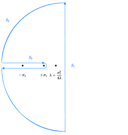
Fix with , we need to evaluate the Fourier-Mellin integral of the form
In other words, we need to know the integral along the line segment in Fig 1. First, we observe that the function
| (2.11) | ||||
| (2.12) |
has a simple pole at . Therefore using the Cauchy Residue Theorem, we have,
| (2.13) |
Second, we evaluate the integral over the arc . Parametrize the by with , therefore
| (2.14) |
and thus for any fixed
| (2.15) |
For the part of the integral , one can show that
| (2.16) |
and thus with some universal constant
| (2.17) |
Putting these estimates together and sending , we have shown
| (2.18) |
Third, we evaluate the integral over the segment (corresponding to the branch point of ), with where . We consider this since the function is a well-defined single-valued function only on . One can show that
| (2.19) | |||
| (2.20) | |||
| (2.21) | |||
| (2.22) |
Finally, we integrate over the semi-circular arc in . Parametrizing , we have, . In turn, the integral reduces to
We note that this integral converges to zero as . Putting three pieces together, we conclude the proof. ∎
We next turn our attention to . Recall , and set . Differentiating, we obtain that , defined in (2.1). Coupled with (2.4), we have, satisfies the integro-differential equation,
| (2.23) | ||||
Lemma 2.2.
The function has Laplace transform
Proof of Lemma 2.2.
Taking Laplace transforms in (2.23), we obtain,
where we set . Transposing, we obtain,
Recall that , and thus . This allows us to obtain the Laplace transform of . Finally we note that by direct computation, . This completes the calculation.
∎
We set . Let denote the largest real solution to the equation .
Lemma 2.3.
If , we have that
Proof.
By definition,
We first claim that there exists a constant such that
We establish each bound in turn. Set with , and note that . Choose small enough so that , since by assumption. Thus we have,
This remains bounded as . To analyze the second term, first observe from Lemma 2.1 that
Thus for any , there exists large enough such that for all ,
Then we have, setting with small enough,
The control of this term is complete once we control the two integrals above. To this end,
which remains bounded as . Finally,
which remains bounded as .
Finally, we turn to the term . Recall that, using (2.5), , where
Further recalling that , we have
| (2.24) |
where is the remainder term which we will later show to be bounded as . Computing the first term, we obtain,
| (2.25) |
Note that involves two terms and remains bounded when since
Thus, the proof is complete on establishing that remains bounded as .
We note that may be expressed as the sum of three terms, denoted as , where
is the same as above except the roles of and are reversed, and the third term is defined as below:
Now the support of is upper bounded by and in the range of integration. Thus, we may upper bound by
which remains bounded when . Similarly, can be bounded. Applying a similar trick, can be bounded by
and this once again remains bounded as . Putting everything together and from (2), we have the desired result.
∎
We now turn to the proof of Theorem 1.2.
Proof of Theorem 1.2.
First, using (1.6), we have,
If is a real root of , is a real root of the fixed point equation . In turn, such a root exists if and only if , which immediately gives us the desired conclusion.
Consider first the regime . Observe that (2.5) implies,
Further, Lemma 2.3 implies that as along a sector,
Thus Lemma 2.2 implies
Thus using [3, Lemma 7.2],
Noting that , we have,
To simplify this, first note that . Calculating the exact value of this derivative we obtain that
Equating these for yields that
Putting things together,
Now note that , so the final limit becomes
It remains to analyze the sub-critical regime . Using Lemma 2.2, we note that has a simple pole at . Thus there exists such that
| (2.26) |
In turn, this implies
This completes the proof in this sub-case, as immediately in this case.
Finally, we focus on the case . Lemma 2.1 implies that in this case. On the other hand, in this case . Thus using Lemma 2.2, we note that the leading asymptotics of is determined by the pole at . Specifically, , which concludes the proof.
∎
3 Proof of Theorem 1.1
Setting , the dynamics under the rotated coordinate system can be expressed as
| (3.1) |
Setting , we note that Eqn. (3.1) reduces to
| (3.2) |
Utilizing this expression, one can verify that takes the following integral form
| (3.3) | ||||
| (3.4) |
We first re-express the solution of our SDE.
Lemma 3.1.
Define . Then we have,
| (3.5) |
Proof.
The proof follows by an application of the integration by parts formula on the solution (3.3). ∎
Definition 3.2.
We define the empirical measure
| (3.6) |
where the fourth marginal is an empirical distribution on the path space .
Consider the following collections of functions, with domain space and range space one of for :
Finally, define
| (3.7) |
All functions in have the same domain. To simplify notation, for elements in , we use to mean evaluated at for a generic point . Similarly for elements in and .
Define and note that for , We introduce the following convention: for a discrete set and a function , . The next result establishes that for all , depend on through the statistics .
Lemma 3.3.
There exist functions
such that
| (3.8) |
Proof.
To this end, we combine (3.5) with the definition of to get a fixed point equation
| (3.9) |
This implicitly specifies the function . The corresponding equation for is more involved. To track this representation systematically, we recall the representation of the solution from (3.5), and denote , where the represent the respective terms in the RHS of (3.5). Now, recall that , and therefore
| (3.10) |
We argue that the RHS above is a continuous function of , and . To this end, we record these terms explicitly. Define
| (3.11) |
First, we present the “diagonal” terms.
Next, we present the “off-diagonal” terms.
This specifies the function implicitly.
∎
Given Lemma 3.3, we next establish that , are, in fact, functions of the low-dimensional statistics .
Lemma 3.4.
There exist functions
such that
To this end, our main strategy is to apply a Picard iteration scheme on the fixed point equations (3.8). We start with some initial guess , , and carry out the iterative updates
| (3.12) |
We will show that this iteration system is contractive, and thus identify , as the unique fixed points of this system. In this endeavor, we will utilize the precise form of the functions , as described in the proof of Lemma 3.3. First, we need some preliminary estimates.
Lemma 3.5.
Recall that , defined in (1.2), is non-negative and Lipschitz. Then we have that
-
(i)
for any , .
-
(ii)
For any , , .
-
(iii)
For any ,
(3.13) -
(iv)
For any , ,
-
(v)
With probability 1, there exist , (possibly random), depending on such that
(3.14)
Proof of Lemma 3.5.
The parts (i)-(iv) are directly adapted from [3], and are just collected here for the convenience of the reader. We prove (v). Note that
This implies
Thus there exists (possibly random), independent of , such that
Iterating this bound in , we obtain
This completes the proof. ∎
Proof of Lemma 3.4.
First observe that for any ,(3.9) implies
This implies, using Lemma 3.5, there exists a constant such that
| (3.15) |
To control the second term, we observe,
which directly implies
Plugging this back into (3.15), there exists (independent of ) such that
Analyzing the iterative update equation for , one can derive a similar bound.
| (3.16) |
Iterating these bounds, it follows that there exists such that
Thus the iteration is contractive, and the fixed point system (3.8) has a unique fixed point for each . This completes the proof. ∎
Finally, we will establish that derived in Lemma 3.4 are continuous functions. To this end, recall that
We equip , , with the sup-norm topology. Further, we equip with the product topology. With this notion of convergence, we can establish the following continuity properties of and .
Lemma 3.6.
The maps and are continuous.
Proof.
We measure the discrepancy between and using the uniform topology on this space, and denote . Define , via the fixed point equations
Observe that
Controlling the second term, we note from (3.9) that
On the other hand, using the same argument as in the proof of Lemma 3.4, we have that
Combining, we obtain,
Thus there exists such that
Thus is Lipschitz. The argument for is analogous, and thus omitted. This completes the proof. ∎
Our next lemma establishes that under the two initial conditions introduced in Section 1, the low-dimensional statistics converge almost surely to deterministic limits. We defer the proof of this lemma to Section 3.1.
Lemma 3.7.
Under the i.i.d. and i.i.d. under rotated basis initial conditions, each element in converges to deterministic limits almost surely.
Proof of Theorem 1.1.
Fix . Lemma 3.4, 3.6 and 3.7 together imply that , converge to deterministic functions and respectively. It remains to characterize these limits. Note that from (3.3),
| (3.17) | ||||
| (3.18) |
We recall that and , and that , uniformly. Thus calculating , and setting , we obtain the desired fixed point equations in the limit. Note that the final limit operation requires that converges to the claimed limits under the i.i.d. and rotated i.i.d. initial conditions. This completes the proof. ∎
3.1 Proof of Lemma 3.7
We prove Lemma 3.7 in this section. Note that for , , . Thus in the lemma above, we mean specifically that converges almost surely as a -valued random variable. Throughout, we equip with a sup-norm.
Proof.
Before embarking on a formal proof, we summarize our general proof strategy. The proof follows in two stages–first, we establish that for any fixed , converges almost surely. We next prove an additional Holder continuity property of , uniformly in , that allows us to bootstrap the above pointwise a.s. convergence to a functional a.s. convergence statement.
We first consider the case of the initial condition (ii). Here, almost sure convergence of for any fixed follows immediately from the Strong Law of Large Numbers. We next establish that for sufficiently large , the following holds for each element of : there exists , independent of , such that almost surely, for any ,
| (3.19) |
Before we delve into the proof, we argue that (3.19) suffices to establish convergence of to in sup-norm.
To see this, first observe that for every , , by the explicit form of these functions. Thus is uniformly continuous on . This implies that if we fix , there exists such that whenever , we have that
Define and fix any . Let denote a -net of . For any , if we denote to be the nearest point in the net, we know that for sufficiently large ,
| (3.20) | ||||
Since the RHS does not depend on , and can be arbitrary as long as , we have the required sup-norm convergence of as a function on . We shall next establish Holder continuity of (uniformly in ), that is, property (3.19) for each .
To begin, let us consider . Observe that
| (3.21) | ||||
where the last inequality is true a.s. with independent of N only for sufficiently large on using the SLLN. Thus is Lipschitz almost surely for sufficiently large . For the above upper bound, recall that we always have for sufficiently large. Similar arguments work for , , , so we skip presenting those details here.
We next turn to . Recall that
where the last equality follows from the orthogonality of the matrix . Recall that . This implies
| (3.22) |
using standard deviation bounds for the supremum of a Brownian motion and a Chernoff bound on . This completes the proof for .
Next, we move to functions in . First note that for , we have that on , by the Uniform Law of Large Numbers and properties of Brownian Motion. Next, we present the proof for —the proofs for and are similar. To show Holder continuity of , set . Then we have,
Thus for any ,
There exists such that almost surely, , . Further, , and
Thus there exists constants such that almost surely,
where the last inequality follows from the fact that , so that we always have . The other functions in may be controlled using analogous arguments.
Finally, we move onto the functions in . We sketch the proof for ; the same proof works for , . Set . Thus we have, for ,
| (3.23) | |||
almost surely for some universal constants . This completes the proof for initial condition (ii).
Next, we turn to the initial condition (i). The main difference now lies in the fact that the pointwise almost sure convergence no longer follows directly from SLLN for all choices of . First, we observe that the difference in initial conditions only affects , , and —thus we can restrict to these specific functions. We will use the same strategy to establish functional almost sure convergence, starting from the pointwise a.s. convergence, thus we omit those details. We present the proof for –the proofs for are similar. Fix . We have,
| (3.24) |
where we use . We observe that
since entries of are i.i.d. with mean . Now, there exists such that occurs eventually almost surely. Given and , . Moreover,
Thus on the event , for any ,
for some universal constant . The proof is complete on using the Borel Cantelli lemma.
∎
References
- ABUZ [18] Elisabeth Agoritsas, Giulio Biroli, Pierfrancesco Urbani, and Francesco Zamponi. Out-of-equilibrium dynamical mean-field equations for the perceptron model. Journal of Physics A: Mathematical and Theoretical, 51(8):085002, 2018.
- ACHL [19] Sanjeev Arora, Nadav Cohen, Wei Hu, and Yuping Luo. Implicit regularization in deep matrix factorization. Advances in Neural Information Processing Systems, 32, 2019.
- ADG [01] G Ben Arous, Amir Dembo, and Alice Guionnet. Aging of spherical spin glasses. Probability theory and related fields, 120(1):1–67, 2001.
- ADT [20] Alnur Ali, Edgar Dobriban, and Ryan Tibshirani. The implicit regularization of stochastic gradient flow for least squares. In International conference on machine learning, pages 233–244. PMLR, 2020.
- AG [97] G Ben Arous and Alice Guionnet. Symmetric langevin spin glass dynamics. The Annals of Probability, 25(3):1367–1422, 1997.
- AG [98] Gerard Ben Arous and Alice Guionnet. Langevin dynamics for sherrington-kirkpatrick spin glasses. In Mathematical aspects of spin glasses and neural networks, pages 323–353. Springer, 1998.
- AGJ [20] Gerard Ben Arous, Reza Gheissari, and Aukosh Jagannath. Algorithmic thresholds for tensor pca. The Annals of Probability, 48(4):2052–2087, 2020.
- AGJ [21] Gerard Ben Arous, Reza Gheissari, and Aukosh Jagannath. Online stochastic gradient descent on non-convex losses from high-dimensional inference. Journal of Machine Learning Research, 22(106):1–51, 2021.
- AKT [19] Alnur Ali, J Zico Kolter, and Ryan J Tibshirani. A continuous-time view of early stopping for least squares regression. In The 22nd international conference on artificial intelligence and statistics, pages 1370–1378. PMLR, 2019.
- BADG [06] Gérard Ben Arous, Amir Dembo, and Alice Guionnet. Cugliandolo-kurchan equations for dynamics of spin-glasses. Probability theory and related fields, 136(4):619–660, 2006.
- BAGJ [20] Gérard Ben Arous, Reza Gheissari, and Aukosh Jagannath. Bounding flows for spherical spin glass dynamics. Communications in Mathematical Physics, 373(3):1011–1048, 2020.
- BAP [05] Jinho Baik, Gérard Ben Arous, and Sandrine Péché. Phase transition of the largest eigenvalue for nonnull complex sample covariance matrices. The Annals of Probability, 33(5):1643–1697, 2005.
- BGN [11] Florent Benaych-Georges and Raj Rao Nadakuditi. The eigenvalues and eigenvectors of finite, low rank perturbations of large random matrices. Advances in Mathematics, 227(1):494–521, 2011.
- [14] Antoine Bodin and Nicolas Macris. Model, sample, and epoch-wise descents: exact solution of gradient flow in the random feature model. Advances in Neural Information Processing Systems, 34, 2021.
- [15] Antoine Bodin and Nicolas Macris. Rank-one matrix estimation: analytic time evolution of gradient descent dynamics. In Conference on Learning Theory, pages 635–678. PMLR, 2021.
- BRT [19] Mikhail Belkin, Alexander Rakhlin, and Alexandre B Tsybakov. Does data interpolation contradict statistical optimality? In The 22nd International Conference on Artificial Intelligence and Statistics, pages 1611–1619. PMLR, 2019.
- CB [20] Lenaic Chizat and Francis Bach. Implicit bias of gradient descent for wide two-layer neural networks trained with the logistic loss. In Conference on Learning Theory, pages 1305–1338. PMLR, 2020.
- CBS+ [20] Chiara Cammarota, Giulio Biroli, Stefano Sarao, Lenka Zdeborova, and Florent Krzakala. Who is afraid of big bad minima? analysis of gradient-flow in a spiked matrix-tensor model. In 33rd Conference on Neural Information Processing Systems (NeurIPS 2019), Vancouver, Canada, volume 33, 2020.
- CCM [21] Michael Celentano, Chen Cheng, and Andrea Montanari. The high-dimensional asymptotics of first order methods with random data. arXiv preprint arXiv:2112.07572, 2021.
- CK [93] Leticia F Cugliandolo and Jorge Kurchan. Analytical solution of the off-equilibrium dynamics of a long-range spin-glass model. Physical Review Letters, 71(1):173, 1993.
- CL [21] Niladri S Chatterji and Philip M Long. Finite-sample analysis of interpolating linear classifiers in the overparameterized regime. Journal of Machine Learning Research, 22(129):1–30, 2021.
- CLB [21] Niladri S Chatterji, Philip M Long, and Peter L Bartlett. When does gradient descent with logistic loss find interpolating two-layer networks? Journal of Machine Learning Research, 22(159):1–48, 2021.
- CS [92] Andrea Crisanti and H-J Sommers. The sphericalp-spin interaction spin glass model: the statics. Zeitschrift für Physik B Condensed Matter, 87(3):341–354, 1992.
- DG [21] Amir Dembo and Reza Gheissari. Diffusions interacting through a random matrix: universality via stochastic taylor expansion. Probability Theory and Related Fields, 180(3):1057–1097, 2021.
- DGM [07] Amir Dembo, Alice Guionnet, and Christian Mazza. Limiting dynamics for spherical models of spin glasses at high temperature. Journal of Statistical Physics, 126(4):781–815, 2007.
- DKT [19] Zeyu Deng, Abla Kammoun, and Christos Thrampoulidis. A model of double descent for high-dimensional binary linear classification. arXiv preprint arXiv:1911.05822, 2019.
- DLZ [21] Amir Dembo, Eyal Lubetzky, and Ofer Zeitouni. Universality for langevin-like spin glass dynamics. The Annals of Applied Probability, 31(6):2864–2880, 2021.
- DS [20] Amir Dembo and Eliran Subag. Dynamics for spherical spin glasses: disorder dependent initial conditions. Journal of Statistical Physics, 181(2):465–514, 2020.
- [29] Suriya Gunasekar, Jason Lee, Daniel Soudry, and Nathan Srebro. Characterizing implicit bias in terms of optimization geometry. In International Conference on Machine Learning, pages 1832–1841. PMLR, 2018.
- [30] Suriya Gunasekar, Jason D Lee, Daniel Soudry, and Nati Srebro. Implicit bias of gradient descent on linear convolutional networks. Advances in Neural Information Processing Systems, 31, 2018.
- Gru [96] Malte Grunwald. Sanov results for glauber spin-glass dynamics. Probability theory and related fields, 106(2):187–232, 1996.
- Gru [98] Malte Grunwald. Sherrington-kirkpatrick spin-glass dynamics. In Mathematical Aspects of Spin Glasses and Neural Networks, pages 355–382. Springer, 1998.
- JM [20] Hui Jin and Guido Montúfar. Implicit bias of gradient descent for mean squared error regression with wide neural networks. arXiv preprint arXiv:2006.07356, 2020.
- JT [19] Ziwei Ji and Matus Telgarsky. The implicit bias of gradient descent on nonseparable data. In Conference on Learning Theory, pages 1772–1798. PMLR, 2019.
- LRZ [20] Tengyuan Liang, Alexander Rakhlin, and Xiyu Zhai. On the multiple descent of minimum-norm interpolants and restricted lower isometry of kernels. In Conference on Learning Theory, pages 2683–2711. PMLR, 2020.
- LS [20] Tengyuan Liang and Pragya Sur. A precise high-dimensional asymptotic theory for boosting and minimum--norm interpolated classifiers. arXiv preprint arXiv:2002.01586, 2020.
- MBB [18] Siyuan Ma, Raef Bassily, and Mikhail Belkin. The power of interpolation: Understanding the effectiveness of sgd in modern over-parametrized learning. In International Conference on Machine Learning, pages 3325–3334. PMLR, 2018.
- MBC+ [20] Stefano Sarao Mannelli, Giulio Biroli, Chiara Cammarota, Florent Krzakala, Pierfrancesco Urbani, and Lenka Zdeborová. Marvels and pitfalls of the langevin algorithm in noisy high-dimensional inference. Physical Review X, 10(1):011057, 2020.
- MKUZ [19] Stefano Sarao Mannelli, Florent Krzakala, Pierfrancesco Urbani, and Lenka Zdeborova. Passed & spurious: Descent algorithms and local minima in spiked matrix-tensor models. In international conference on machine learning, pages 4333–4342. PMLR, 2019.
- MKUZ [20] Francesca Mignacco, Florent Krzakala, Pierfrancesco Urbani, and Lenka Zdeborová. Dynamical mean-field theory for stochastic gradient descent in gaussian mixture classification. Advances in Neural Information Processing Systems, 33:9540–9550, 2020.
- MRSY [19] Andrea Montanari, Feng Ruan, Youngtak Sohn, and Jun Yan. The generalization error of max-margin linear classifiers: High-dimensional asymptotics in the overparametrized regime. arXiv preprint arXiv:1911.01544, 2019.
- MWCC [18] Cong Ma, Kaizheng Wang, Yuejie Chi, and Yuxin Chen. Implicit regularization in nonconvex statistical estimation: Gradient descent converges linearly for phase retrieval and matrix completion. In International Conference on Machine Learning, pages 3345–3354. PMLR, 2018.
- MZ [20] Stefano Sarao Mannelli and Lenka Zdeborová. Thresholds of descending algorithms in inference problems. Journal of Statistical Mechanics: Theory and Experiment, 2020(3):034004, 2020.
- NLG+ [19] Mor Shpigel Nacson, Jason Lee, Suriya Gunasekar, Pedro Henrique Pamplona Savarese, Nathan Srebro, and Daniel Soudry. Convergence of gradient descent on separable data. In The 22nd International Conference on Artificial Intelligence and Statistics, pages 3420–3428. PMLR, 2019.
- SHN+ [18] Daniel Soudry, Elad Hoffer, Mor Shpigel Nacson, Suriya Gunasekar, and Nathan Srebro. The implicit bias of gradient descent on separable data. The Journal of Machine Learning Research, 19(1):2822–2878, 2018.
- SMU [21] Stefano Sarao Mannelli and Pierfrancesco Urbani. Analytical study of momentum-based acceleration methods in paradigmatic high-dimensional non-convex problems. Advances in Neural Information Processing Systems, 34, 2021.
- SZ [81] Haim Sompolinsky and Annette Zippelius. Dynamic theory of the spin-glass phase. Physical Review Letters, 47(5):359, 1981.
- SZ [82] Haim Sompolinsky and Annette Zippelius. Relaxational dynamics of the edwards-anderson model and the mean-field theory of spin-glasses. Physical Review B, 25(11):6860, 1982.
- ZBH+ [21] Chiyuan Zhang, Samy Bengio, Moritz Hardt, Benjamin Recht, and Oriol Vinyals. Understanding deep learning (still) requires rethinking generalization. Communications of the ACM, 64(3):107–115, 2021.